the Creative Commons Attribution 4.0 License.
the Creative Commons Attribution 4.0 License.
 | 09 Feb 2023
Spatio-temporal analysis of slope-type debris flow activity in Horlachtal, Austria, based on orthophotos and lidar data since 1947
Florian Haas
Tobias Heckmann
Moritz Altmann
Fabian Fleischer
Camillo Ressl
Sarah Betz-Nutz
Michael Becht
In order to get a better understanding of the future development of alpine slope-type debris flows in the frame of climate change, complete and gapless records of the last century for this type of geomorphologic process are necessary. However, up to now such records have been scarce. Here, the slope-type debris flow activity in Horlachtal, Austria, has been investigated since 1947 with the help of historic and recent area-wide remote sensing data. Using geomorphological mapping, both spatial and temporal variabilities in debris flow dynamics can be shown. The results indicate short-term variations rather than consistent increasing or decreasing trends of slope-type debris flow activity in Horlachtal. Specifically, three active periods between 1954 and 1973, 1990 and 2009, as well as 2015 and 2018, can be registered. Analyses of the deposited debris flow volumes show that for parts of the study area the largest volumes appeared in the early 1990s, which might have even influenced the dynamics in the following years. Studies on the spatial variabilities revealed differences of slope-type debris flow activity within the study area and point to local rainfall events as triggers. However, long-term precipitation data of high temporal resolution of two alpine meteorological stations do not reveal increasing or decreasing trends in the occurrence of such events.
- Article
(6758 KB) - Full-text XML
- BibTeX
- EndNote


Debris flows are gravitational mass movements consisting of granular solids mixed with water that can reach high velocities (Varnes, 1978) and occur in mountainous regions around the world as natural hazards (Dowling and Santi, 2014). In high-alpine regions, this process is of great importance for the sediment budget (Heckmann et al., 2012; Curry et al., 2006; Rainato et al., 2017; Hilger, 2017; Theule et al., 2012), as they couple sediment sources on slopes with alpine streams (Heckmann and Schwanghart, 2013; Iverson, 2012). Therefore, debris flows are a very important process in high-alpine geomorphology and landscape evolution, as a change in debris flow activity has a high impact on sediment balances. In alpine environments, debris flows initiated in torrent beds (torrent bed type or channel type) can be distinguished from debris flows initiated on slopes (slope-type or hillslope debris flows). These types not only differ in various geomorphic characteristics like flow length, drainage area or slope values (Chen et al., 2009) but also show different initiation mechanisms (Sassa, 1984).
Because of their importance for high-alpine geosystems, there are many attempts trying to model debris flows in order to predict their appearance, velocities or ranges (Wichmann, 2017; Turnbull et al., 2015; Wu, 2015). But the changing environmental parameters caused by climate change (Nogués-Bravo et al., 2007; Beniston, 2005, 2003) might have an impact on debris flow occurrence and properties and must hence be accounted for in modelling efforts. Therefore, in order to predict debris flow dynamics in the future, it is necessary to understand debris flow behaviour in the past and especially in the last few decades that witnessed the most intense climatic changes. However, there are not many studies containing (near) complete debris flow records beyond the last few decades in alpine catchments. Some authors have used historical documents to reconstruct debris flow events (D'Agostino and Marchi, 2001; Tropeano and Turconi, 2004), but there are great uncertainties, especially for earlier periods (Marchi and Tecca, 2006). In addition, these archives often do not cover smaller debris flows and high-altitude regions far from settlements and focus primarily on channel-type debris flows. Other methods for reconstructing debris flow activities include dendrogeomorphology (Lopez Saez et al., 2011; Stoffel, 2010; Bollschweiler et al., 2008) or lichenometry (Helsen et al., 2002; Innes, 1983). However these methods depend on the presence of suitable vegetation and are only partly useable above the treeline. The usage of area-wide lidar (light detection and ranging) data as a basis for determining debris flow activity can reveal past debris flow events at higher resolution (Dietrich and Krautblatter, 2017; De Haas and Densmore, 2019), but the availability of these data is restricted to the last 2 decades and thus in a period which is entirely dominated by climate change. Aerial images and orthophotos are used to detect changes in alpine environments and are available on an area-wide basis back to ca. 1950 for most regions of the Alps (Bayle, 2020; Altmann et al., 2020; Fleischer et al., 2021). Because they cover whole catchments in great detail, historical and recent orthophotos are used to detect and date debris flow processes (Jomelli et al., 2007, 2003; Dietrich and Krautblatter, 2017).
A synthesis of previous studies on the historical long-term development of debris flows shows that the results are not univocal. Dietrich and Krautblatter (2017) show an enhanced debris flow activity in Plansee, Austria, since the 1980s when investigating the debris flow activity between 1947 and 2010. Other studies seem to confirm an increase in debris flow frequency when considering a long investigation period (Winter, 2020; Pelfini and Santilli, 2008; Kiefer et al., 2021). Due to changes in sediment supply, Hirschberg et al. (2021) stated that the number of debris flows in Illgraben in Switzerland will decrease. However, several studies have revealed no trends in debris flow activity besides short-term fluctuations (Stoffel et al., 2014, 2005; Stoffel, 2010; Bollschweiler and Stoffel, 2010; Lopez Saez et al., 2011; Bollschweiler et al., 2008).
This paper aims to not only analyse slope-type debris flows in a temporal way but also in a spatial way within an alpine catchment. Through this spatio-temporal view we want to better understand the characteristics of these mass movement processes using methods that provide information on both scales. Thus, we establish a slope-type debris flow record in Horlachtal in the central Alps of Austria between 1947 and 2020 using historical and recent orthophotos, as well as lidar elevation models. The work is based on a precise mapping of all recognizable debris flows since 1947, which allows process frequencies to be derived. Process magnitudes are obtained from lidar data, as well as from an established area–volume relationship of debris flow deposits (Hilger, 2017; Larsen et al., 2010; Bennett et al., 2012). The debris flow volumes are correlated with parameters of the respective hydrological catchment areas in order to improve the understanding of spatial differences in debris flow activity. Because high-intensity rainfall events are decisive for the initiation of debris flows in the study area, this paper aims to analyse the spatial and temporal differences in slope-type debris flow activity in Horlachtal with the help of temporal high-resolution precipitation data. Thus, we want to gain a better understanding of the process behaviour throughout the past 7 decades and link the results to changes in precipitation patterns due to the changing climate.
Horlachtal is located in the northern part of the central Alps (Fig. 1) and forms a side valley of the Ötztal. It is drained by the Horlachbach River, which flows over the Stuibenfall waterfall into the main stream of the Ötztal (Ötz). Horlachtal itself can be subdivided into three north–south striking tributary valleys (Grastal – GT, Larstigtal – LT and Zwieselbachtal – ZT) in addition to the east–west striking main valley (HT), as well as the tributary valleys, Finstertal (FT) and Weites Kar (WK) (Table 1). The main outflow of the valley is captured by a gauging station in Niederthai, which is located close to the area outlet at Stuibenfall. Another gauging station is operated by the Tyrolean Hydropower Company (TIWAG) at Horlachalm, where part of the discharge is captured by a Tyrolean weir and fed to the Finstertal Reservoir near Kühtai via underground tunnel systems in order to use it for hydropower.
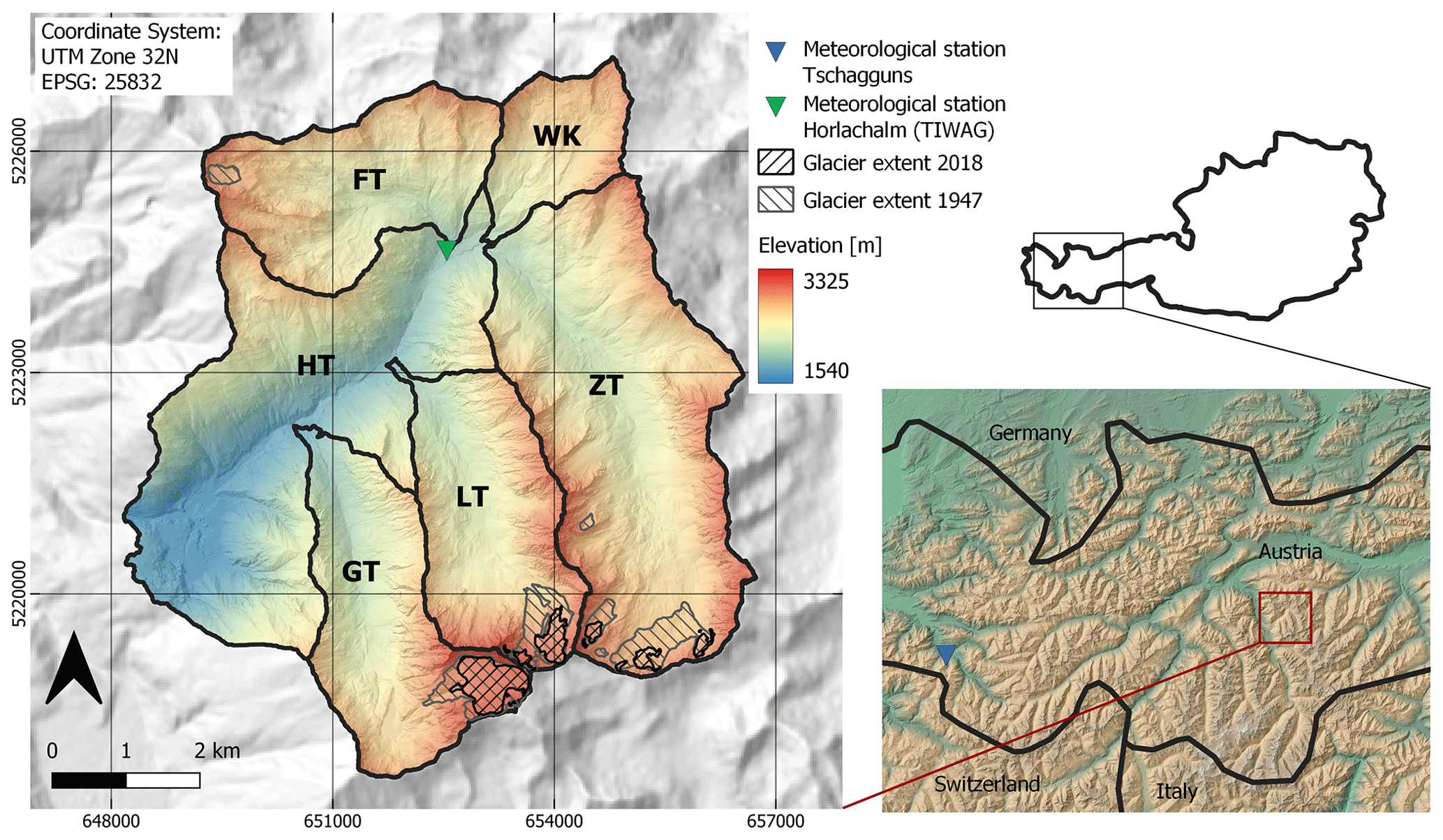
Figure 1Location of Horlachtal in the Stubai Alps. The study area is divided into the sub-catchments main valley (HT), Grastal (GT), Larstigtal (LT), Zwieselbachtal (ZT), Weites Kar (WK) and Finstertal (FT). Shown glacier extents were mapped based on orthophotos of the corresponding years. Elevation data of the study area are based on airborne lidar data from 2019. Large-scale elevation data in the background are based on the ALOS global digital surface model © JAXA.
Table 1Attributes of the different sub-catchments in the study area based on airborne lidar data of 2017 (Province of Tyrol).
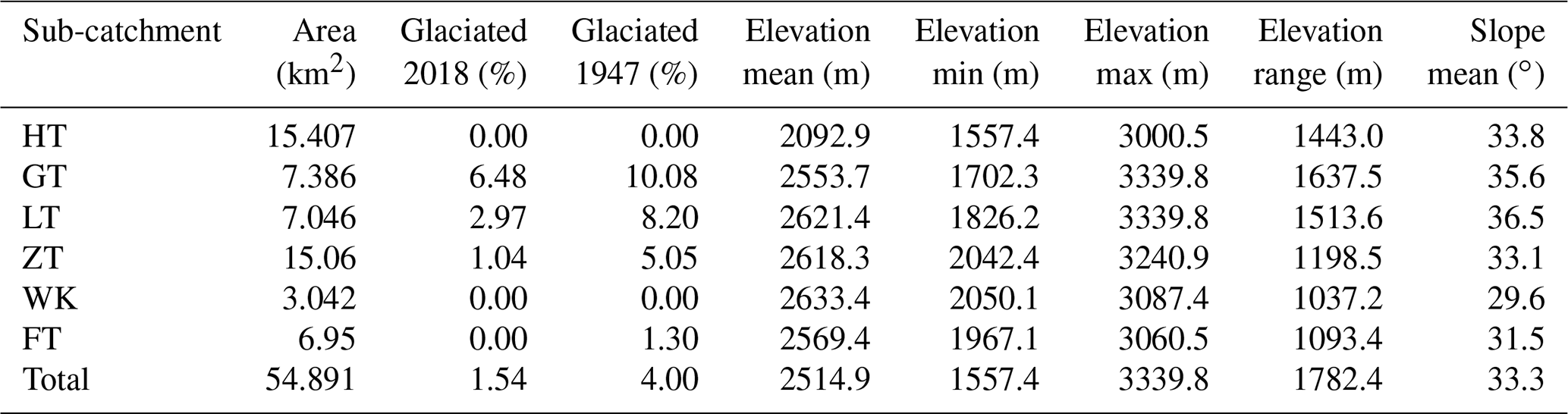
Horlachtal spans elevations of 1557 to 3340 m and shows a typical altitudinal alpine gradation of the vegetation with the treeline at about 2200 to 2300 m. About 1.54 % of the area is currently glaciated, with Grastalferner as the biggest glacier (ca. 0.48 km2) in the study area, whose outflow is buffered by Grastalsee. Horlachtal shows the typical geomorphic process dynamics of high-mountain regions, including rock glaciers in the upper areas, which testify to the presence of permafrost.
Geologically, the study area is located in the Ötztal Massif with predominant gneisses and mica schists, which strike in an east–west direction parallel to the main valley (Geitner, 1999; Becht, 1995). Due to their tectonic history, the rocks are very susceptible to weathering, which leads to high rockfall activity and ample availability of debris for debris flows, which led to the formation of in part very large debris cones.
Because of its location in the central Alps, the Horlachtal Valley is protected from advective precipitation so that the annual total of precipitation here is lower than for example in the northern Alps (Geitner, 1999; Becht, 1995). The mean annual precipitation between 1990 and 2019 adds up to 817 mm, which mostly occurs during the summer months (Fig. 2). The mean annual temperature within the same timeframe is 3.1 ∘C at the meteorological station Horlachalm (1910 m, all elevation data throughout this study refer to ellipsoid elevations; see Fig. 1 for the location within the study area; data courtesy of the Tyrolean Hydropower Company, TIWAG).

Figure 2Climate diagram of the Horlachalm station (1910 m) using temperature and precipitation data between 1990 and 2019. Upper dashed lines represent 75 % percentiles; lower dashed lines show the 25 % percentiles. Data source: TIWAG.
The debris flows in Horlachtal, which are analysed here, can be described as slope-type debris flows with starting zones at the contact area between steep bedrock and the adjacent talus slope. The hydrological catchments of these debris flows are developed in the steep bedrock sections where rainwater is concentrated and further discharges into the slope (Zimmermann, 1990; Rieger, 1999; Wichmann, 2006; Rickenmann and Zimmermann, 1993).
The influence of the morphometry of the hydrological catchment of a slope-type debris flow can be decisive with regard to its activity and magnitude (Becht and Rieger, 1997; De Haas and Densmore, 2019; Dietrich and Krautblatter, 2019; Marchi et al., 2019; Shen et al., 2012; Wilford et al., 2004) and should be taken into account when analysing magnitudes of debris flows. The debris flow material originates on the one hand from glacial moraine material covered with rockfall debris on the talus slopes. On the other hand, it emerges from rockfall deposits temporarily stored in the bedrock catchments. The debris flows in Horlachtal occur in transport-limited hillslope systems and are triggered by high-intensity precipitation events of about 20 mm in 30 min (Becht, 1995; Becht and Rieger, 1997). In contrast to other types of debris flow systems, the initiation of debris flows on the slopes of the study area is not affected by pre-event conditions like antecedent rainfall, as the necessary runoff is formed in bedrock areas. The most important driving factors for debris flow initiation in Horlachtal are thus high rainfall intensities that generate high peaks of surface runoff.
3.1 Debris flow inventory using orthophotos
The basis for all further evaluation methods was the multi-temporal mapping of individual debris flows since 1947 in the whole study area. Debris flow inventories already existed especially in LT and ZT (Rieger, 1999; Thiel, 2013; Heckmann et al., 2014), which were carefully checked and updated using historical and recent orthophotos. All orthophotos used for this purpose and their characteristics are listed in Table 2. In some years, the aerial images do not cover the entire study area. The missing regions were supplemented with aerial images from other flight campaigns with a temporal divergence of 1 to 3 years. The coverage of the individual campaigns can be viewed in the Laser- und Luftbildatlas Tirol of the Province of Tyrol (https://lba.tirol.gv.at/public/karte.xhtml, last access: 26 January 2023). The original aerial images of 1947, 1953, 1954, 1970 and 1973 were available from the archives of the Province of Tyrol. The scanned aerial images were oriented and calibrated in a bundle block adjustment (McGlone et al., 2004) using ground control points. These points were manually identified in recent data (orthophoto and digital elevation model) by looking for unique features (mostly rocks) in stable areas. After the bundle block adjustment, a digital surface model was derived by means of image matching and used to create an orthophoto mosaic for the mentioned years. The remaining referenced orthophotos were taken from the web map service of the Province of Tyrol (https://www.data.gv.at, last access: 26 January 2023).
Table 2Attributes of orthophotos used for debris flow mapping. Date of data acquisition for each time step, which covers most of the study area, is marked in bold.
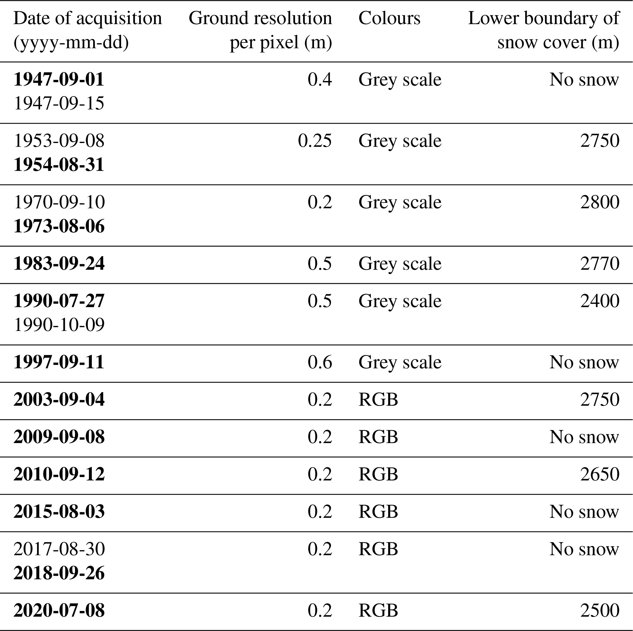
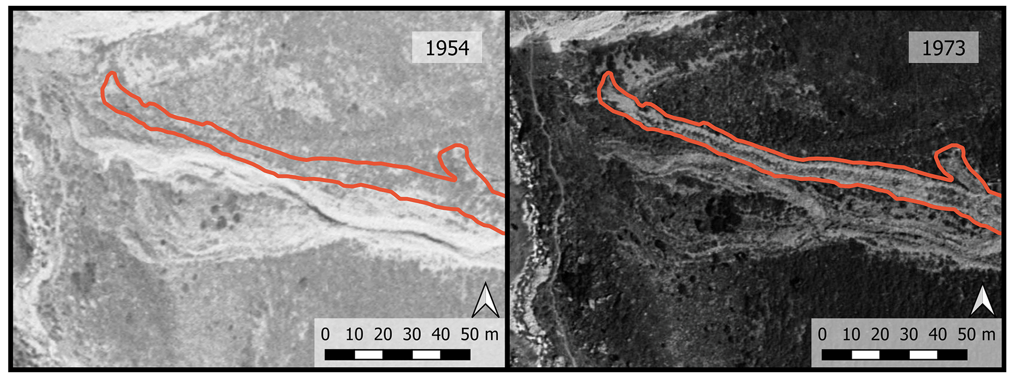
Figure 3Example of the mapping process. The mapped debris flow (encircled in red) must have happened between the acquisition of the orthophotos 1954 (no debris flow landforms) and 1973. Sources of aerial images: Office of Metrology and Surveying and the Province of Tyrol.
Since the mapping is influenced by subjective interpretation of the orthophoto, it was done by one and the same person; visible typical debris flow deposits on the talus slopes were digitized into polygon shapefiles. In addition to the deposits, the starting zones in the aerial photographs were determined using the visible erosion areas. For debris flows with a hydrological catchment in bedrock, these are primarily located in the direct transition from the bedrock area to the adjacent scree slopes (Rieger, 1999). If debris flow-typical process forms (transport channels, levées, deposits) have emerged during the comparison of two consecutive orthophotos, a new debris flow was mapped and dated to the time interval between the dates of image acquisition. The example in Fig. 3 shows debris flow landforms that emerged between 1954 and 1973, the times the shown aerial images were acquired.
The mapping and dating of these individual events were carried out in the entire study area and in all available time intervals. The sub-catchments HT, GT, LT, ZT, WK and FT were considered separately (cf. Fig. 1).
For some periods, not all debris flows could be mapped because of poor image quality in shadowed areas. Due to the sometimes long time intervals between two orthophotos, especially in the first half of the considered time span, two or more debris flow process areas might have overlapped in time and space in such a way that individual events could not be recorded by the mapping. This in turn leads to a possible underrepresentation of debris flows, which is more likely in longer time intervals than in shorter ones.
3.2 Volume measurements
We computed the planimetric area of all debris flow deposits except for those where the depositional zone could not be clearly identified; this was the case with very small events and in shadowed areas.
Because of their high spatial resolution, two different lidar datasets were used to determine debris flow deposition volumes for debris flows which occurred between the single lidar epochs. The first dataset from 2006 was provided by the Province of Tyrol. This dataset is only available as a gridded digital terrain model (DTM; resolution: 1 × 1 m); the initial point cloud was not obtainable. The second lidar dataset was recorded during a field campaign of the University of Eichstätt-Ingolstadt in 2019 using a RIEGL VUX-1LR integrated in a RIEGL VP-1 HeliCopterPod (see http://riegl.com for details, last access: 26 January 2023) with a spatial resolution of 13.1 points m−2 on average. The processing of the raw data included the precise calculation of the trajectory using the data of two different differential GNSS ground stations installed in the study area. A final strip adjustment was done using the approaches of Glira et al. (2015, 2016), which are implemented in the point cloud processing software OPALS (Pfeifer et al., 2014). The outliers of the resulting point cloud were filtered, and the ground points were classified using the extension LIS Pro 3D of Laserdata (Petrini-Monteferri et al., 2009) of the GIS software SAGA (Conrad et al., 2015). As a result, a final DTM (resolution: 1 × 1 m) could be generated. For more details about the processing of the raw point cloud, refer to Rom et al. (2020).
The difference between the two topographic raster datasets DTM of difference (DoD) provided volumetric data for most of those debris flow depositions that occurred between the lidar data acquisitions in 2006 and 2019.
3.2.1 Error assessment of the volume data
Uncertainties in the DTMs of 2006 and 2019 lead to errors in the calculated DoD (Lane et al., 2003; Bakker and Lane, 2017) and thus also in the calculation of the debris flow volumes. In order to minimize the errors in the DoD, the two lidar datasets had to be coregistered. To optimize this processing step, the study area was divided into several smaller areas of interest so that the algorithms for matching the data were able to work on a more local scale. In these regional patches, areas were identified where no geomorphologic changes were expected in between the lidar data acquisitions. These stable areas were mapped as close to the debris flow depositions as possible, and were selected, if possible, to be of similar steepness. As point cloud data were available only for one of the lidar datasets, we coregistered the two gridded DTMs using the approach of Nuth and Kääb (2011) implemented in the Python package pybob (https://pybob.readthedocs.io, last access: 26 January 2023).
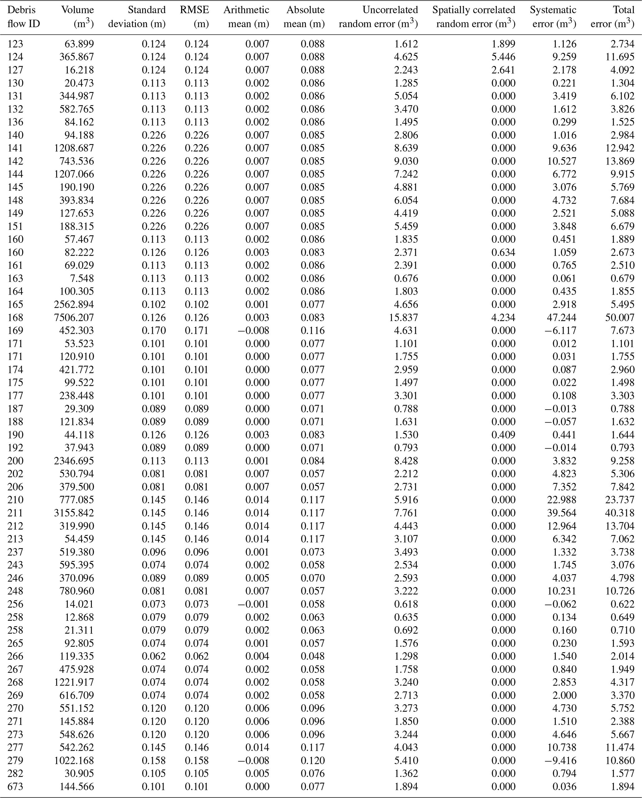
To get a better understanding of the errors, the DoDs within the identified stable areas were analysed regarding the precision (standard deviation) and the accuracy (RMSE – root mean square error), as well as the arithmetic mean and the absolute mean. For a total assessment of the error of the volume of debris flow deposits, the error was calculated following the approach of Anderson (2019), which combines the uncorrelated random error, the spatially correlated random error and the systematic error of the DoD. All debris flow volumes detected from the DoD together with the respective errors are listed in Table A1 in the Appendix.
3.2.2 Volume estimation for debris flows not covered by the DoD
The volumes of those debris flow deposits that are detectable in the DoD were determined in each case by summing up the values of the DoD in the mapped deposition areas. For those debris flow deposits which are not contained in the DoD (especially for debris flows prior to 2006), only the area of the deposits could be mapped using the respective pair of orthophotos. In order to estimate the volume of different types of mass movements based on the accumulation area, numerous studies derived an empirical relationship between the deposit area (A) and the deposit volume (V) (Guzzetti et al., 2009; Magirl et al., 2010; Larsen et al., 2010). This relationship is expressed by a power law with an exponent γ > 0 and the intercept α:
The exponent γ in such area–volume relationships depends not only on the analysed process (e.g. rock fall, landslide, debris flow) but also on its subtypes (Larsen et al., 2010; Griswold and Iverson, 2008). Nevertheless, the range of γ usually seems to be within a similar range for several types of mass movements (Hilger, 2017).
The relationship between the volumes and deposition areas is used in order to predict the volumes of depositions for which only the areas are known. Because in this study only slope-type debris flows of the same type are analysed, and no large differences in the debris material are to be expected, the uncertainties here focus on the individual debris flow processes. These include the different content of water or the topography of the deposition area before the debris flow event.
In order to fit Eq. (1) to the empirical data, a variety of different fitting techniques can be used (see for example Guzzetti et al., 2009; Larsen et al., 2010). One simple method includes a least-squares linear fit to the log-transformed data. Another way of fitting a power-law function to the data is by using non-linear regression. In order to be better comparable to other studies calculating such relationships, both methods were applied in the present study by using the statistical software R and the functions lm (linear model) and nls (non-linear least squares) (Baty et al., 2015).
3.2.3 Uncertainties of debris flow volumes
To get a better understanding of the uncertainties involved in the volume calculations, the goodness of fit of the area–volume models has to be described. However for non-linear correlations, the coefficient of determination R2 is not a valid measure (Spiess and Neumeyer, 2010). Instead, we use the 95 % prediction interval of the non-linear regressions. The upper and lower boundary of the prediction interval for each area were used as the maximum and minimum debris flow volume for those events that were not quantified from the DoD. Where the lower limit of the prediction interval is negative (which occurs especially with small deposit areas), it was set to 0 m3; therefore, the lower uncertainty band of the computed volumes is frequently shorter than the upper. For all debris flows included in the DoD, the uncertainty limits were defined by the error assessment in Sect. 3.2.1. For calculating the uncertainty of the total debris flow volume for each of the considered epochs, the uncertainties of each single volume calculation was propagated. Therefore, the total uncertainty of an epoch is the square root of the sum of the squared single uncertainties (Anderson, 2019).
3.2.4 Magnitude–frequency relationship
The calculated magnitudes, as well as the known ages of the debris flows due to the multi-temporal mapping, allowed us to establish a magnitude–frequency relationship. This has been done for various gravitational processes, such as landslides (Bennett et al., 2012; Gao et al., 2018; Tanyaş et al., 2019; Guzzetti et al., 2009), rockfalls (Ravanel and Deline, 2011), channelized debris flows (Gao et al., 2018) and also slope-type debris flows (Hilger, 2017). Using the poweRlaw package within R (Gillespie, 2015), we calculated an empirical cumulative distribution function (CDF) to represent the relationship between debris flow deposit volumes and their frequencies (Bennett et al., 2012; Hilger, 2017). Subsequently, we were able to fit a continuous power law distribution to the CDF. However, this distribution is only valid for volumes exceeding a minimum magnitude xmin (Bennett et al., 2012), and the calculated exponent of the power law β, which is based on a cumulative distribution, has to be reduced by 1 when compared with non-cumulative exponents (Brunetti et al., 2009; Haas et al., 2012).
3.3 Hydrological catchment parameters and debris flow magnitudes
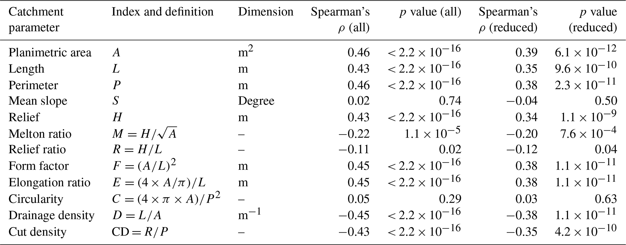
The tool “upslope area” implemented in SAGA-GIS (Freeman, 1991) was used to calculate the hydrological catchment areas for each of the mapped debris flow starting zones based on the DTM of 2019. With the help of spatial analyses of the catchments we derived a number of different parameters that are known as influencing variables for the magnitude and frequency of debris flows (Wilford et al., 2004; De Haas and Densmore, 2019; Zhao et al., 2020; Zhou et al., 2016). These parameters include the area (A) of the hydrological catchment, as well as its length (L), perimeter (P) and mean slope (S). The relief parameter (H) describes the difference between the highest and lowest point of the catchment. The Melton ratio (M) Melton (1957) has been found to correlate with debris flow dynamics (Wilford et al., 2004; De Haas and Densmore, 2019). In addition, relief ratio (R), form factor (F), elongation ratio (E), circularity (C), drainage density (D) and cut density (CD) were calculated according to the definitions in Table 3 (see Sect. 4.3). All of the mentioned parameters were correlated to the respective debris flow volumes using Spearman's rho to see a possible connection between the magnitudes and the morphometry of the hydrological catchments.
Table 3Calculated parameters of the hydrological catchments of the slope-type debris flows alongside their definitions and dimensions. Correlation of each parameter with the respective debris flow volumes were calculated by Spearman's ρ. The p values represent the significance of the correlations. The statistical parameters are shown for the complete dataset (all; n = 404), as well as for the reduced dataset (reduced; n = 296).
3.4 Analysis of precipitation data
Meteorological data are recorded in the study area at the Horlachalm station, operated by TIWAG at an altitude of 1910 m (see Fig. 1). Temporally high-resolution data (measurements every 15 min) have been available for precipitation totals since 1989. Since slope-type debris flows in Horlachtal are transport-limited, the frequency of heavy rainfall should be related to the frequency of debris flow events. Potential triggers are short-term events such as thunderstorms rather than days with high total rainfall (Bernard et al., 2020; Underwood et al., 2016; Pelfini and Santilli, 2008). For Horlachtal, Becht and Rieger (1997), as well as Becht (1995), determined an intensity threshold of 20 mm per 30 min. As the collected data at Horlachalm station only date back to 1989, they cover only a small part of the study period. The meteorological station Längenfeld (provider: BMNT – Bundesministerium für Nachhaltigkeit und Tourismus) is located further down in the Ötztal valley and has been recording meteorological data since the year 1895. However, these data are not used for evaluation in the present work, because the Längenfeld station only records daily totals of precipitation values. Heavy rainfall events of short duration can hardly be reconstructed from daily totals (Pelfini and Santilli, 2008; Jomelli et al., 2007). For example, the statistical evaluation of meteorological data in Altmann et al. (2020) shows that the development of daily totals and heavy rainfall events through several decades can even be opposite. Nevertheless, daily totals are used in most studies to explain long-term debris flow development (Dietrich and Krautblatter, 2017), because there are hardly any alpine meteorological stations measuring hourly or sub-hourly precipitation totals prior to the 1990s. As temporally high-resolution precipitation data are decisive when interpreting long-term debris flow records, it was decided to include the data of the precipitation measuring site Tschagguns (provider: Hydrographischer Dienst Vorarlberg; data available at https://ehyd.gv.at/, last access: 7 February 2023). This station records totals for every minute derived from continuous precipitation data from May 1953 until the end of 2018. It is located approximately 80 km west of the study area at an altitude of 681 m (see Fig. 1), but its location north of the Alpine main divide makes the weather conditions comparable to Horlachtal up to a certain point. Because of the distance between Tschagguns and Horlachtal, the recorded absolute precipitation data cannot simply be transferred, and the extreme precipitation events at Tschagguns are not connected to the debris flow activity in Horlachtal. However, it seems to be promising to analyse trends in high-intensity precipitation patterns since 1953 to get an idea of changes in extreme event patterns for this part of the eastern Alps.
4.1 Spatio-temporal debris flow mapping
In the entire study area, a total of 834 debris flow events were mapped between 1947 and 2020 using historic and recent orthophotos.
Figure 4 shows the spatial distribution of the mapped process areas. It reveals that the debris flows are not homogeneously distributed over the whole study area but are mainly concentrated in the three parallel north–south-oriented sub-catchments GT, LT and ZT. However, since the sub-catchments vary in size and the periods between the aerial image acquisitions are not uniform, the number of slope-type debris flows per square kilometre and year was calculated for better comparison (Fig. 5).
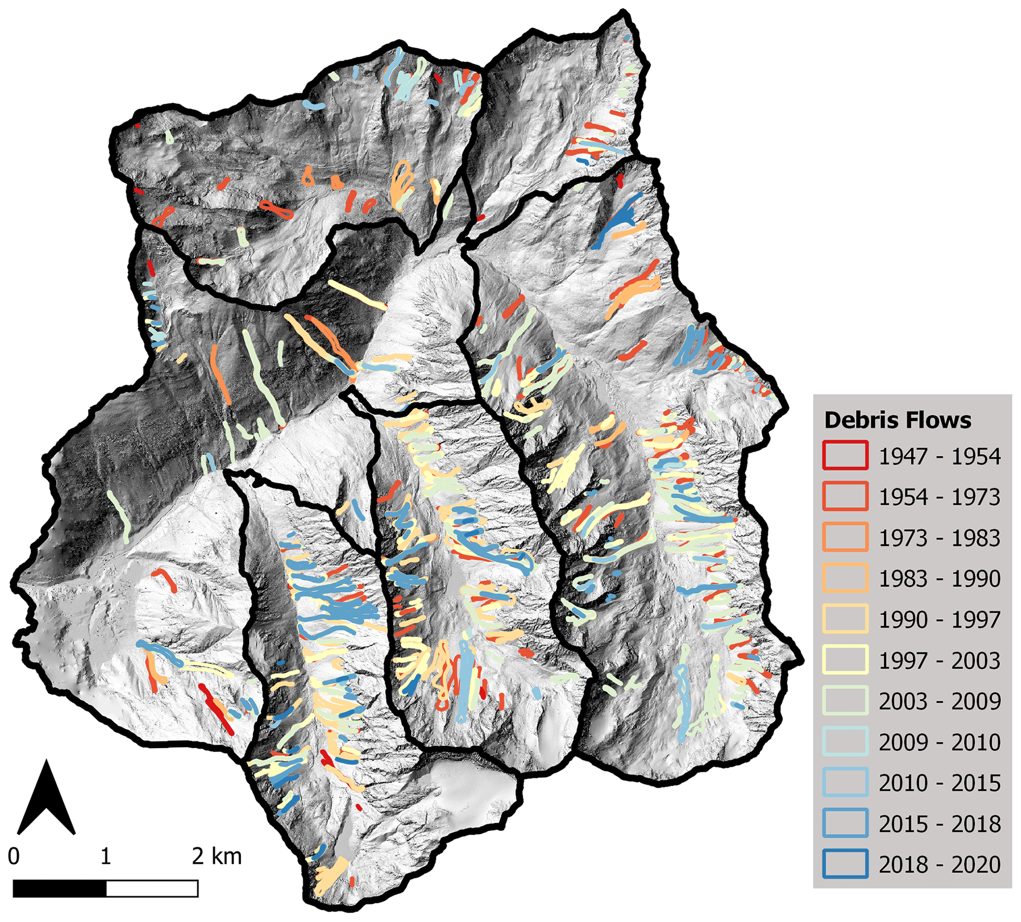
Figure 4Results of the debris flow mapping in the entire study area. More recent debris flows overlay older ones in some places.
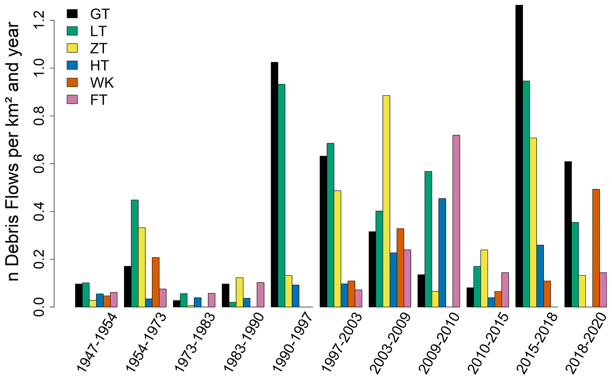
Figure 5Mapped debris flows per square kilometre and year. Distinguished between time intervals and sub-catchments.
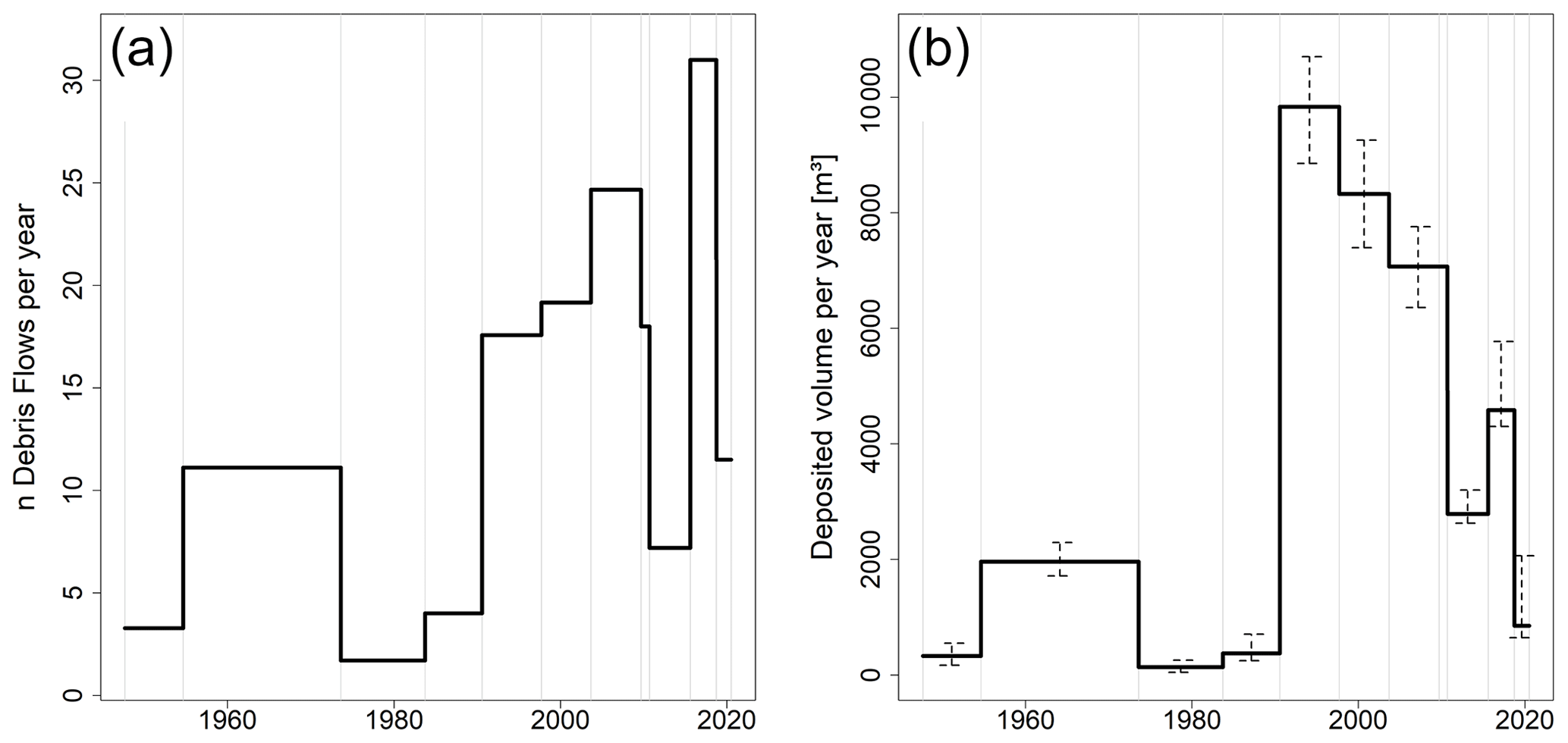
Figure 6Temporal variations of slope-type debris flow activity in Horlachtal since 1947. (a) The number of mapped slope-type debris flows per year. (b) The deposited volume of slope-type debris flows per year. Uncertainties of the calculations are added for each time span. The light grey vertical lines in both panels represent the acquisition dates of the used orthophotos.
The mapped slope-type debris flows show not only spatial differences but also temporal differences. In Fig. 6a, the total number of mapped debris flows in the entire study area (all sub-catchments) for each epoch is depicted. As the time spans of different epochs are not uniform, we calculated the annual frequency of debris flows per year for a better comparison of the process activity throughout the investigated time span. Periods of higher and lower debris flow activity can be observed in Horlachtal. Between 1954 and 1973, significantly more debris flows were triggered in total and per year than in the periods before (1947–1954) and after (1973–1990). The next very active period lasted from 1990 to 2009. However, the highest number of debris flows per year within the observed timeframe occurred between 2015 and 2018.
4.2 Debris flow volumes
The mapping of the debris flows showed a concentration of these processes in the parallel sub-catchments GT, LT and ZT. Those debris flows show a quite different picture in terms of frequency and especially magnitude when comparing them to the activity in the other sub-catchments. Most of the debris flow deposits in HT are hidden under dense vegetation in the remote sensing data, and thus a precise mapping of the accumulation area there is not possible. In addition, in WK and FT, the few debris flows that have been detected are of such small magnitudes that we have not been able to delineate the depositional area sufficiently from the orthophotos. Because of these reasons and because of the similarities in the geomorphological and geographical settings, the analyses concerning deposition volumes were carried out exclusively in GT, LT and ZT.
4.2.1 Area–volume relationship
For a total of 58 debris flows it was possible to map the deposition area in the DoD from the 2006 and 2019 terrain models with sufficient accuracy to enable a balance of the deposition volumes (Appendix A1). The volumes range from very small (7.55 m3) to large debris flows (7506 m3). With the help of this data, a relationship between the area and volume of debris flow deposits could be established which follows a power law (Fig. 7). The exponent γ in Eq. (1) could be calculated as γ=1.21 for the fitted linear model. This method tries to fit a linear model to the log-transformed area and log-transformed volume data. The log scaling of both of the input data results in a distortion of the residuals, which are used in the fitting process.

Figure 7Relationship between area and volume of debris flow deposits in GT, LT and ZT. The 95 % prediction interval of the model calculated by the non-linear method is shown with the dashed lines.
In order to reduce this bias, a non-linear model was fitted using the nls() function in R. This approach determines the non-linear least-squares estimates of the parameters of a power-law model (Bates and Watts, 1988) and results in a mathematical best fit with respect to the residuals. The exponent of the fitted non-linear model results to be slightly lower with for the 95 % confidence interval. In the non-linear model plotted in Fig. 7, it is shown that the model slightly overestimates volumes for areas < 500 m2. Again, this is due to the log scaling of the axes.
With the help of the regression of volume on area, the debris flow volume could be calculated for all events with a precisely delimited deposit. In total, the deposition volumes could be calculated (based on the DoD) or estimated (area ∼ volume) for 404 debris flows in GT, LT and ZT. The uncertainties of the volume calculations were carried out as described in Sect. 3.2.3.
Figure 6b reports the annual debris flow volume per epoch. Similar to the mapping results in Fig. 6a, the debris flow volumes show periods with high and low deposition rates per year. Most remarkable is the sudden and strong increase in volumes in the period 1990–1997 compared to the previous periods. After years of relatively few debris flows with little deposited material, the many triggered processes between 1990 and 1997 also transported an above-average amount of material.
Comparable to the mapping results, the volume data of the time intervals between 1954–1973 and 1990–2010 reveal increased deposition, but the period between 2015 and 2018 produced less deposited volume than one could have assumed from the very high number of triggered debris flows in that time interval. Thus, it can be stated that although many events occurred, they have deposited relatively little sediment in total.
4.2.2 Magnitude–frequency relationship
The calculated magnitude–frequency relationship is shown in Fig. 8. About 70 % of all debris flows in GT, LT and ZT have an accumulated volume above 100 m3, and about 20 % of all debris flows exceed a volume of 1000 m3. Extreme events, which account for less than 1 % of all debris flows, can reach volumes of more than 10 000 m3. The magnitude–frequency relationship can be described by a continuous power-law distribution with an exponent of β=2.9 for volumes of m3 and above and therefore is especially usable for large debris flow volumes.
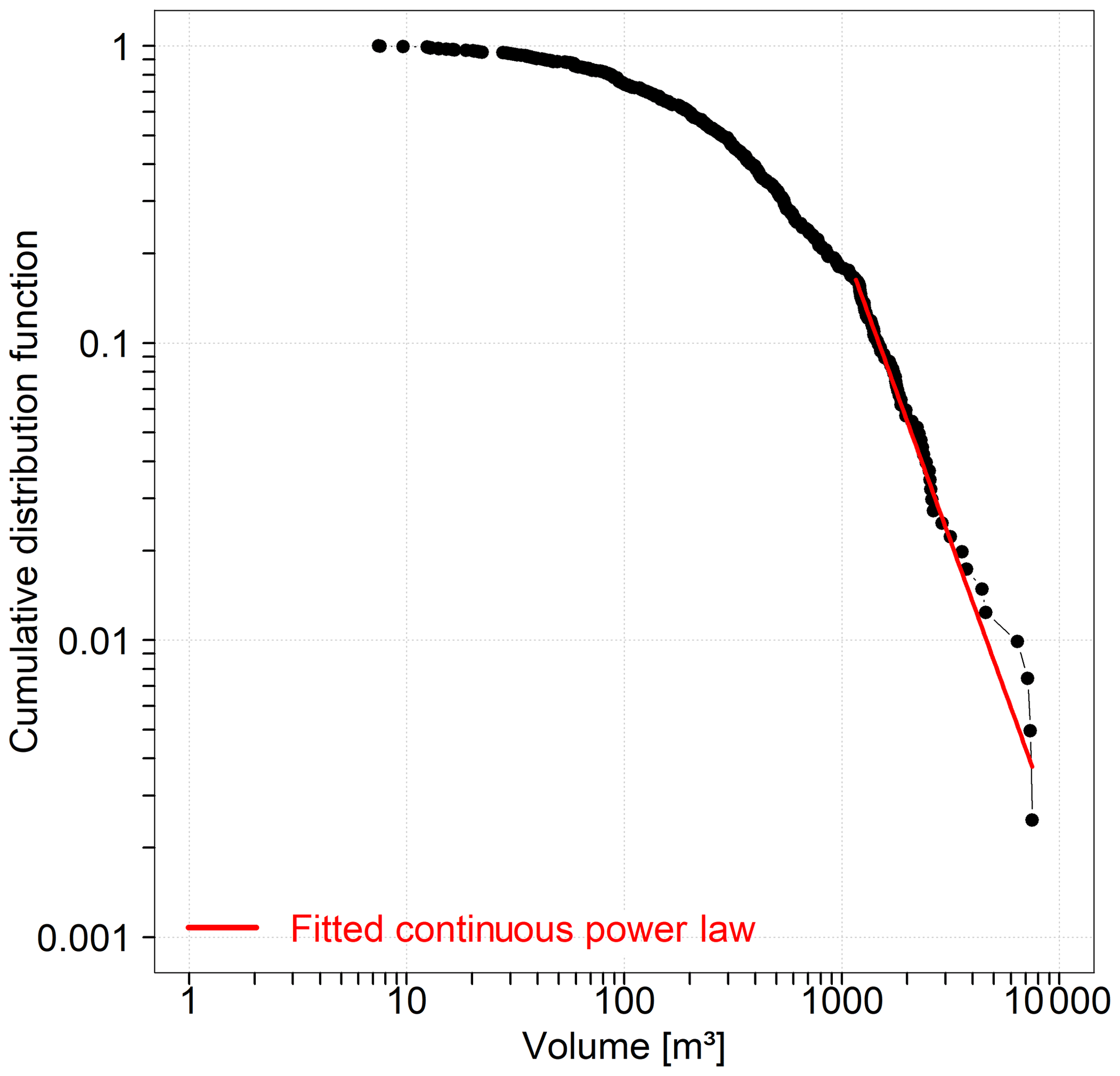
Figure 8Magnitude–frequency relationship displayed with a cumulative distribution function for the debris flows in GT, LT and ZT. The fitted continuous power law describes the relationship for debris flows with a volume greater than 1025 m3.
4.3 Analysis of hydrological catchment parameters
For all 404 debris flows for which the volume could be determined, we performed a correlation analysis of the volumes with various parameters of the respective hydrological catchment areas. In addition, the same statistical analyses were conducted only for the debris flows of those catchments that produced at least two debris flows between 1947 and 2020. For this reduced dataset, the sample size is decreased to 296 debris flows (Table 3).
Although no variable shows a very strong (positively or negatively) correlation, Spearman's rho points in both datasets to slightly positive interrelationships between debris flow volumes and A, L, P, H and F, as well as E. In addition, D and CD indicate a negative correlation in the same order of magnitude. Especially the variables S and C on the other hand have no visible influence on the debris flow volumes. However, this analyses show that the morphometry of the hydrological catchments indeed has an influence on the slope-type debris flow magnitudes.
4.4 Precipitation analysis
For the initiation of debris flows in Horlachtal, high-intensity rainfall events with a large amount of precipitation within a short time are necessary. Therefore, the precipitation data of the stations Horlachalm and Tschagguns were analysed regarding high-intensity events. In Fig. 9, the recorded rainfall data are shown in millimetres per 30 min for both stations. In order to determine a possible increasing or decreasing trend in rainfall events reaching high intensities within a short time interval, all days on which 10 mm per 30 min was exceeded were marked in the records of both stations. The exact magnitude of this threshold is not of great importance, because it is only used in order to get an idea about possible trends in high-intensity rainfall events. As the threshold of 20 mm per 30 min turned out to be exceeded quite rarely in both rainfall records, it was set to 10 mm per 30 min. However, the frequency of these extreme events does not show statistically significant increases or decreases as can be seen in Fig. 9.
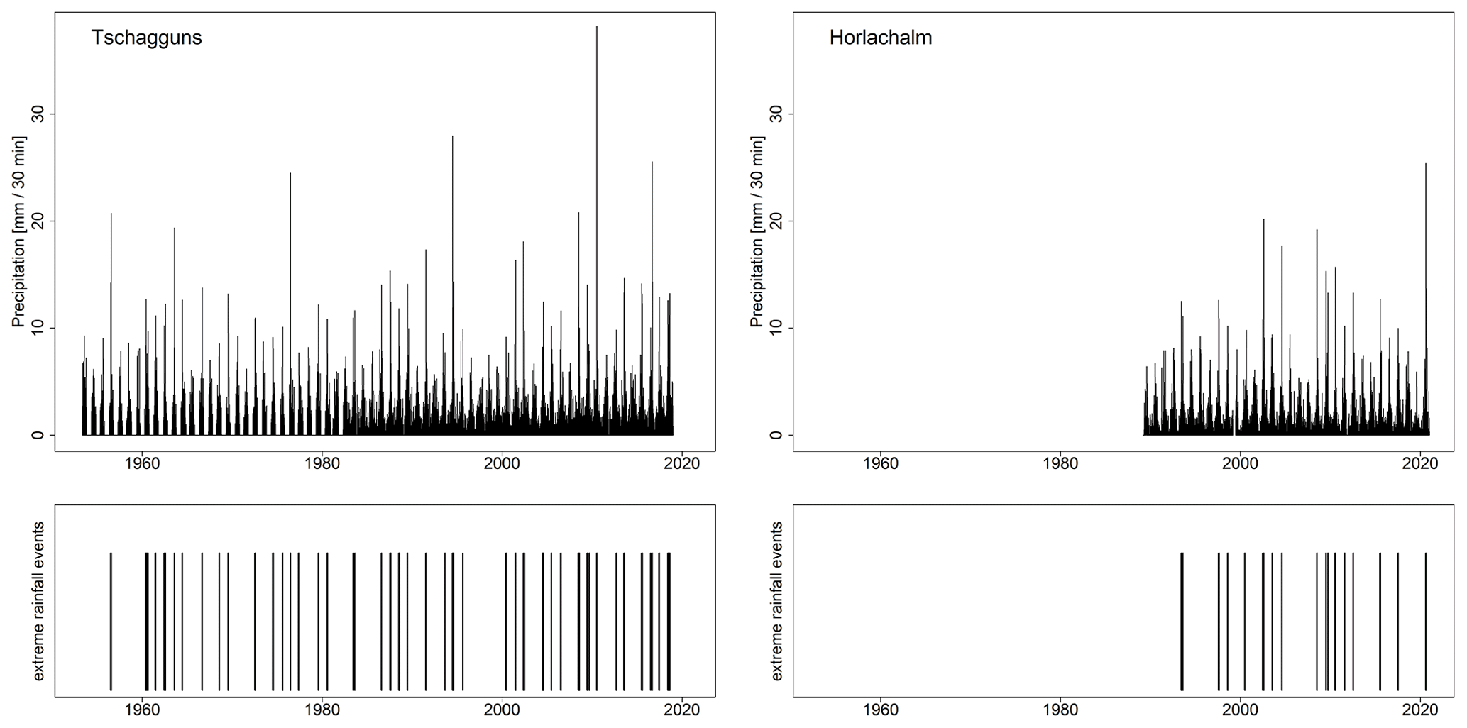
Figure 9Recorded precipitation data of the meteorological stations Tschagguns and Horlachalm. Days with intensities exceeding 10 mm per 30 min are marked in the respective bottom plots.
The cumulative sums of days with a high-intensity rainfall event exceeding 10 mm per 30 min for both stations are shown in Fig. 10. On average, there are slightly more such events per year recorded at Tschagguns station (1.093) than at Horlachalm station (0.831). Nevertheless, there are hardly any periods with particularly many or few events that stand out. The longest time without an event at Tschagguns is nearly 5 years between 28 August 1995 and 14 June 2000 and at Horlachalm almost 4 years between 5 August 2004 and 26 June 2008. But temporal trends of more or few events per year are not detectable at Tschagguns nor at Horlachalm.
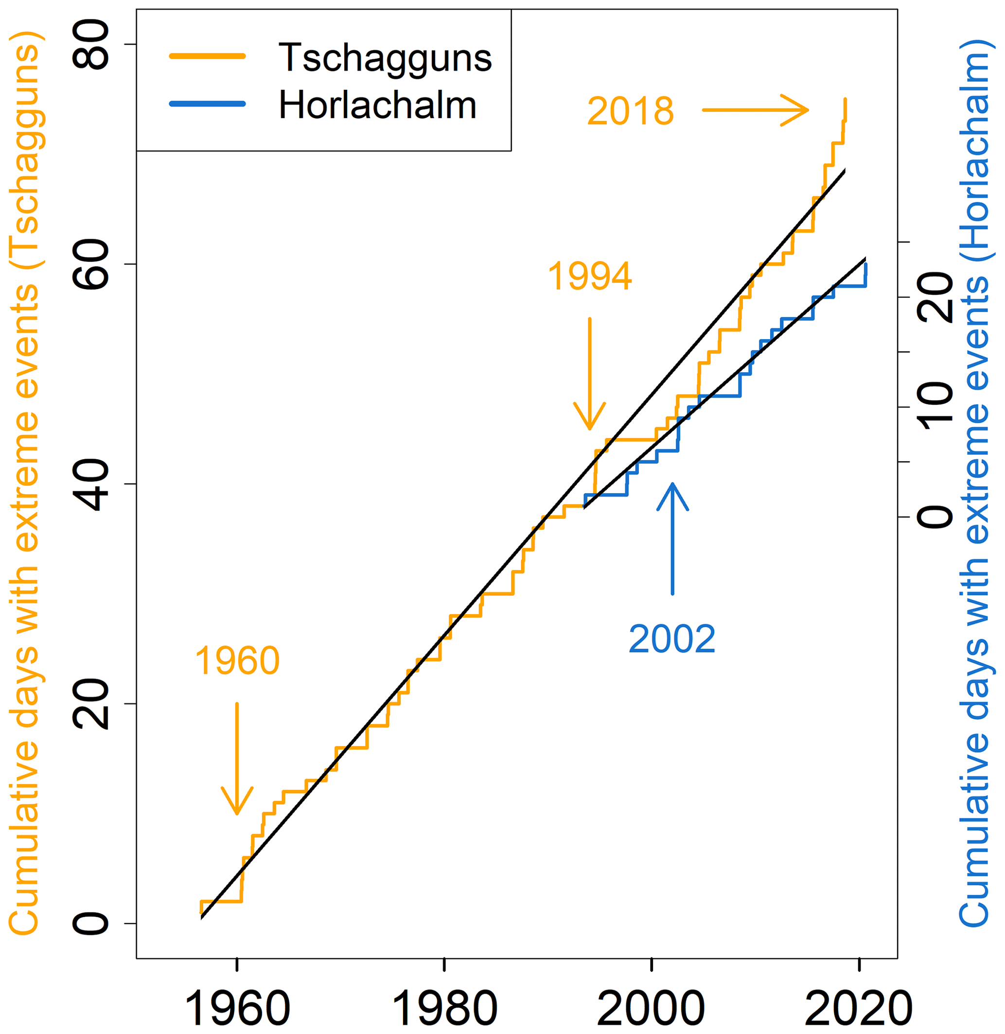
Figure 10Cumulative sums of days with precipitation intensities exceeding 10 mm per 30 min for Tschagguns (orange) and Horlachalm (blue). Years with exceptionally many days with a high-intensity event (Tschagguns: four per year; Horlachalm: three per year) are marked.
5.1 Spatial variability of slope-type debris flows
5.1.1 Topographic variability
The biggest factor for the concentration of debris flow processes in the sub-catchments GT, LT and ZT is probably the presence of catchments in the steep bedrock above large talus cones, which is typical for slope-type debris flows (Rieger, 1999). Rainwater concentrates at the contact zone between these catchment areas and the slope sediments underneath and potentially triggers debris flows. These catchment morphometries are especially pronounced in GT, LT and ZT.
In these very active and north–south-oriented sub-valleys, 68 % of the active debris flow catchments face west, while only 32 % face east. Becht (1995) attributes this difference to the emergence of cirques in the Pleistocene on east-exposed slopes. West-exposed ones do not show these landforms. Therefore, the stepped profiles on east-exposed slopes caused by the cirques prevent the accumulation of high peak discharges during a rainfall event because of a buffering effect of these cirques. Depending on the amount of loose material in the cirques, these buffering effects can cause longer or shorter delays of the runoff and therefore lower the peak discharge. In addition, the slopes beneath the cirques lack rockfall material supply, which otherwise works as suitable material on the slopes for debris flow initiation.
5.1.2 Rainfall variability
It is noticeable that in certain time intervals some sub-catchments were significantly more affected by debris flows than other sub-catchments (see Fig. 5). This is most obvious in the period between 1990 and 1997, when the two neighbouring valleys GT and LT show a strongly increased debris flow activity, especially in comparison to the other sub-catchments. Other time intervals (2003–2009, 2009–2010) also show that some sub-catchments were obviously more affected than neighbouring ones. We attribute these findings to the fact that debris-flow-triggering heavy rainfall events often occur during intense convective and thus spatially restricted thunderstorms (Underwood et al., 2016; Berti et al., 2020; Stoffel et al., 2005) that often affect only parts of the study area.
5.1.3 Effect of debris flow catchment parameters
The results of the correlation of the debris flow volumes and the parameters of the respective hydrological catchments in Table 3 indicate that the catchment morphometry is affecting the spatial variability of slope-type debris flows in Horlachtal. Only a few debris flow studies implemented analyses regarding catchment parameters, and most of them deal with different debris flow types and scales than this study (Becht and Rieger, 1997; Wilford et al., 2004; Marchi et al., 2019; Li et al., 2015).
However, the results of this study match the findings of De Haas and Densmore (2019), who worked in a roughly comparable setting in the United States and found statistically significant correlations between debris flow lobe volumes and A, L, P, H and M. This fits our data just as well as the lack of correlation with S, C and R. The only differences are with the variables F and E, which show a stronger relationship in Horlachtal compared to the results in De Haas and Densmore (2019). In addition, a positive correlation between slope-type debris flow volumes and A was detected by Rieger (1999) in LT as well.
5.1.4 Other factors for debris flow initiation
The starting points of the vast majority of the debris flows in Horlachtal are located at the contact zone between the bedrock catchments and the adjacent talus slopes. Apart from precipitation and the catchment morphometrics, only the slope gradient is of great importance for debris flow initiation here (Becht, 1995). For the present type of debris flow, a slope threshold of about 27∘ at the starting zones can be found in the literature (Rickenmann and Zimmermann, 1993; Dikau et al., 2019). In Horlachtal, these slope gradients range between 22 and 72∘, with 96 % of the starting points exceeding the threshold of 27∘.
Other factors like vegetation cover or soil properties are of minor importance for debris flow initiation in the study area. Most of the starting points are located above the treeline (96.5 % above 2200 m and 92 % above 2300 m). Thus, no trees or higher vegetation grow in the bedrock catchments even at altitudes below the treeline, as the morphodynamics are too high there. In addition, if there is any soil formation in the catchments, it consists only of shallow initial soils because of the same reasons.
5.2 Temporal variability of slope-type debris flows
5.2.1 Frequencies and magnitudes in different periods
Relationship between frequency and magnitude
With the help of the area–volume relationship we were able to calculate deposit volumes, which are necessary to establish a relationship between frequency and magnitude. The resulting exponent of γ=0.92 of the nls() method connecting volumes and areas is comparable with the result of Hilger (2017), who used a linear regression method for slope-type debris flows in Kaunertal (γ=1.08). Furthermore, it is consistent with other comparable studies (Jaboyedoff et al., 2020; Larsen et al., 2010; Guzzetti et al., 2009). The established relationship enabled detailed frequency–magnitude analyses. There are rarely any other studies that calculate such a magnitude–frequency relationship only for debris flows and especially slope-type debris flows. Other papers often focus on debris flows in general (Hungr et al., 2008; Riley et al., 2013). An exception is Hilger (2017), who performed such a calculation in a similar geological setting using slope-type debris flows at Kaunertal, Tyrol. While the general shape and β are very much comparable to this study, the magnitudes of debris flows in Horlachtal are larger by an order of a magnitude. Thus, the largest debris flows in Kaunertal show a volume of about 1000 m3, whereas in Horlachtal the volumes can reach nearly 10 000 m3 (Fig. 11a). In addition, a slight shift of debris flow magnitudes could be detected in Horlachtal. The debris flows of the second half of the investigated time span (1983–2020) reach very high volumes more often than debris flows of the first half (1947–1983) (Fig. 11a).
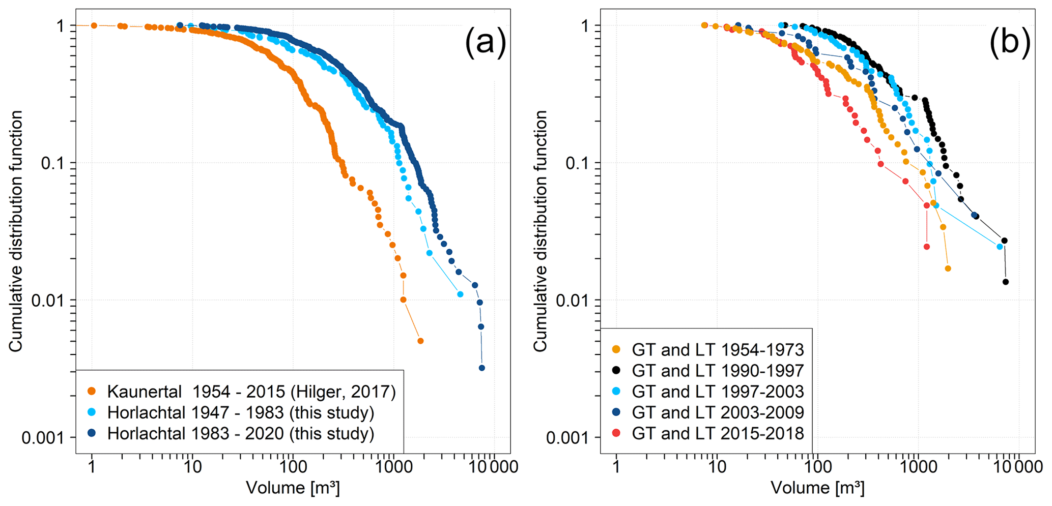
Figure 11(a) Magnitude–frequency relationship for the early debris flows in Horlachtal (1947–1983, light blue) compared with recent debris flows (1983–2020, dark blue). The results of a similar investigation from Hilger (2017) in Kaunertal are shown in orange. (b) Comparison of the magnitude–frequency relationships of different periods in GT and LT.
Temporal development of slope-type debris flow activity
In Horlachtal, the multi-temporal mapping of debris flows, as well as the volumetric measurements, resulted in periods with higher activity (1954–1973, 1990–2010 and 2015–2018) and lower activity in between (Fig. 6a). A consistent linear trend is not recognizable, although it seems that in periods with low activity, the number of debris flows has been rising since 1947. This finding might be biased because of two limitations. First, the most recent orthophotos (especially since 2003) are of very good quality, especially in terms of spatial resolution, light conditions and extent of snow cover. These circumstances allow even small events to be detected and mapped. The second reason is the aforementioned difference in time span lengths, which results in the underestimation of detected debris flows in longer periods.
The mapping results, as well as the calculated deposition volumes, indicate no long-term change in debris flow activity in the past 70 years but with some short-term variabilities. This matches other debris flow records in the Alps (Bollschweiler and Stoffel, 2010; Bollschweiler et al., 2008; Jomelli et al., 2007). Kiefer et al. (2021) detected significant changes over substantially longer time periods when reconstructing the debris flow activity of the past 4000 years based on turbidite measurements of a fan delta. But even in this record, no significant change within the last century is recognizable. In Horlachtal, three periods of increased slope-type debris flow activity can be recognized based on the total number of detected processes (see Fig. 6a): between 1954 and 1973, from 1990 to 2009, and from 2015 to 2018. However, the exact datings of the upper and lower boundaries of the periods with enhanced and low debris flow activity described in this study are predetermined by the used method for establishing the process record. This means that the dates of the acquisition of the aerial images predefine and distort the period boundaries to some extent. In order to delineate the “real” active and inactive periods with higher accuracy, further analyses on the dating of single debris flow events, e.g. by using dendrogeomorphology (Stoffel, 2010), might provide more detailed insights.
A particularly large debris flow event was reported for 31 July 1992, mainly affecting GT and LT (Becht, 1995). These statements can be supported by the debris flow mapping of this study, as many events could be detected in the period 1990–1997 especially in GT and LT (see Fig. 5). In the two subsequent periods until 2009, many events can still be registered in GT and LT but with a decreasing tendency. This could indicate that the large debris flow event in 1992 still had some kind of impact on the debris flow activity of the following years due to the disturbance of the system like e.g. destruction of vegetation or channel deepening. Such a kind of impact on subsequent periods could only be detected for the 1992 event. The high debris flow activities between 1954–1973 and 2015–2018 did not show this pattern of aftereffects, at least not for the temporal resolution predetermined by the orthophotos.
Debris flow magnitude comparison of highly active periods
An indication of the outstanding significance of the 1992 event in GT and LT compared to 1954–1973 and 2015–2018 can be provided by considering the debris flow magnitudes. Figure 11b shows that the deposited debris flow volumes of the period 1990–1997 (which includes the 1992 event) are significantly higher in comparison with the magnitudes of 1954–1973 and 2015–2018. In addition, Fig. 11b shows a slightly decreasing tendency in deposited debris flow volumes from 1990–2009, which in turn supports the aforementioned impact of the 1992 event on the following years.
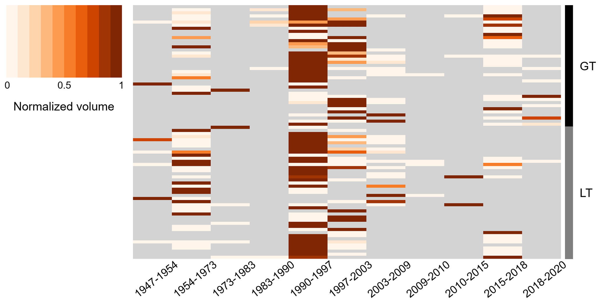
Figure 12Heatmap of the 82 different starting zones in GT and LT, which were triggered at least twice between 1947 and 2020. The normalized magnitudes of every starting zone are shown by the colouring scheme. For more details refer to the text.
In the heatmap of Fig. 12, each row represents one slope-type debris flow starting zone in GT or LT, which was active at least in two different periods between 1947 and 2020. For each individual starting zone (each row of the heatmap), the magnitudes were normalized between 1 (largest event of the starting zone; dark colouring) and 0 (smallest event of the starting zone; light colouring). If no debris flow could be detected at a starting zone in a specific period, the respective colour was set to grey. The heatmap shows that out of the 82 different starting zones in GT and LT which were active at least twice, the largest debris flow event could be detected within the period 1990–1997 on 42 occasions; 73 % of the starting zones produced their maximum deposited volume between 1990 and 2009, however showing a decreasing tendency. Only on 11 different occasions could the largest debris flows be detected in the period 1954–1973, and within 2015–2018 only four starting zones produced their largest event of the total considered timeframe.
The results of the magnitude comparisons of the most active periods indicate a strong influence of the 1990–1997 event, as it produced the largest debris flow volumes in GT and LT by far. This in turn supports the assumption that the debris flows of 1992 (Becht, 1995) affected the debris flow activity in GT and LT for the following years, and the system needed some time to reach the state of before 1990.
The highly active period 1990–2009 with the highest debris flow magnitudes might have affected the debris flow system for even longer. The discrepancy between the high number of detected debris flows from 2015 to 2018 and the relatively small deposited volumes in the same period possibly points to recharge time effects of debris flow channels, as mentioned in Pelfini and Santilli (2008) and demonstrated in Jakob et al. (2005, 2020) and Berger et al. (2011). During the highly active period (1990–2009) the rockfall storages in the bedrock catchments were depleted in some cases. Thus, the debris flows triggered afterwards showed below-average magnitudes. This in turn indicates a very short-term change from transport-limited to supply-limited systems for some of the debris flow channels.
5.2.2 Precipitation and debris flow activity in Horlachtal
Rainfall events triggering slope-type debris flows can occur very locally (see Sect. 5.1). The precipitation data from the Horlachalm meteorological station can therefore not be related to debris flow processes in the entire Horlachtal. As a consequence, the calculation of triggering thresholds using intensity–duration relationships or other methods (Berti et al., 2020; Segoni et al., 2018) would thus be rather inaccurate. Due to the location of the meteorological station, the data are only set in relation to debris flows in ZT. The threshold value for debris flow triggering of 20 mm per 30 min according to Becht and Rieger (1997) has only been exceeded on 2 d since 1989, namely on 31 July 2002 and 2 July 2009. Nevertheless, the mapping of debris flow processes in ZT since 1947 shows that debris flows have also occurred during periods in which the threshold value of 20 mm per 30 min was not exceeded at the Horlachalm meteorological station. This in turn indicates that a precipitation event < 20 mm per 30 min in the study area can be sufficient to trigger debris flows.
In Fig. 13, all high-intensity rainfall events recorded at the Horlachalm station with precipitation values exceeding 5 mm per 30 min are shown together with the mapped number of debris flows per year in ZT and the calculated deposition volume per year in ZT. The acquisition dates of the orthophotos, which were used for mapping the debris flows, are marked as grey vertical lines in the figure.

Figure 13High-intensity rainfall events exceeding 5 mm per 30 min at the Horlachalm station combined with the number of mapped debris flows per year in ZT (black) and the deposited debris flow volumes per year in ZT (orange). The sub-catchment ZT is located quite close to the Horlachalm meteorological station.
Only very few debris flows were mapped in the period between 1990 and 1997 in ZT. The precipitation data show that between the times of the aerial image acquisition in 1990 and 1997, precipitation events of over 10 mm per 30 min were indeed recorded only rarely, and these few precipitation peaks always remained below 15 mm per 30 min. During that period, the precipitation value of 10 mm per 30 min was exceeded a total of 5 times on four different days. The maximum value is 12.6 mm per 30 min on 28 July 1997.
Between the aerial image acquisition in 1997 and 2003, however, considerably more numbers of debris flows and higher debris flow volumes per year were detected in ZT. The precipitation records also show more extreme rainfall events during this period. Precipitation exceeded the value of 10 mm per 30 min a total of 11 times on six different days. The maximum values are also far above the level of the last period, with a maximum value of 20.2 mm per 30 min on 31 July 2002. Even more debris flow processes per year were mapped in the period between 2003 and 2009.
On 4 d between the acquisition of the aerial images of 2010 and 2015, the value of 10 mm per 30 min was exceeded 6 times. However, the maximum of 13.9 mm per 30 min on 7 July 2015 is again relatively low. During this period, comparatively few debris flows per year were mapped in ZT. In the most recent time step between 2015 and 2018, the threshold value was only reached once at the Horlachalm meteorological station on 10 July 2017. At exactly 10.0 mm per 30 min, the maximum value for this period is relatively low. However, many debris flows per year could be determined in ZT during this time step. The corresponding debris-flow-triggering event cannot be traced in the precipitation data. It is therefore probable that this must have been a very local rainfall event that strongly affected ZT but could only be measured at a lower level at the Horlachalm meteorological station.
In general, a correlation between debris flow activity in ZT and precipitation data at Horlachalm station is recognizable. The highest precipitation intensities per 30 min were recorded in the time steps 1997–2003 and 2003–2009, and many debris flow processes could also be mapped during this epoch in ZT. During the periods 1990–1997 and 2010–2015 the maximum precipitation per 30 min was significantly lower, which is also reflected in the lower number of mapped debris flows per year. Only in the time steps 2015–2018 do the datasets not seem to match. This contrast is interpreted as a further indication for very local rainfall events as triggers of debris flows.
The evaluation of high-intensity rainfall events in combination with the mapped slope-type debris flows has shown that the threshold of 20 mm per 30 min specified by Becht and Rieger (1997) is indeed sufficient to trigger large debris flow events in the study area. However, even lower precipitation intensities seem to be sufficient to start debris flows on very active debris cones.
5.3 Methodological limitations
Geomorphological mapping using historic and recent orthophotos is a suitable tool to generate debris flow records for larger study areas, as presented here. A big advantage is that the aerial images cover the entire study area in great detail. It is therefore possible to generate a near-complete debris flow record. Problems only occur when the quality (in terms of resolution, shadow effects and snow cover) of the used images is poor or more than one debris flow occurs during one epoch, and the process areas overlap. In addition, in some cases it is difficult to identify debris flows in densely vegetated areas, which might lead to a slight underestimation of detected processes in the lower altitudes of the study area. Disadvantages of this method are the sometimes large time spans between the acquisition dates of two consecutive aerial images. This not only leads to an increased probability of overlapping events but also to the quite inaccurate dating of single debris flows. As the durations of different epochs are not equal, the normalized number of debris flows per year was calculated in order to compare the debris flow activity. It has to be mentioned, however, that slope-type debris flows are triggered by single precipitation events. The calculations of “debris flows per year” suggest a uniformly distributed debris flow activity throughout the respective epochs, which is far from reality, and hence these calculations should be treated with caution.
Because of the different durations of the epochs, the debris flow record is slightly biased, as the number of debris flows in longer intervals (e.g. 1954–1973) is likely to be underestimated because of the aforementioned reasons. This can be investigated by deliberately removing orthophotos, mapping events based on the remaining imagery and comparing the resulting map with the complete record. In order to get an idea of the magnitude of debris flow underestimation in longer epochs, a re-mapping of debris flow processes was done in GT and LT, where the orthophotos of 1997 and 2003, as well as 2010, 2015 and 2018, were removed from the record. The number of detected debris flows of this second test mapping was then compared with the number of detected debris flows in the original record (reference) in the same timeframe (Table 4).
Table 4Comparison of the number of detected slope-type debris flows of the test mapping with a reduced number of orthophotos and the original mapping (reference). This mapping was conducted in GT and LT and for the time steps 1990–2009 and 2009–2020.
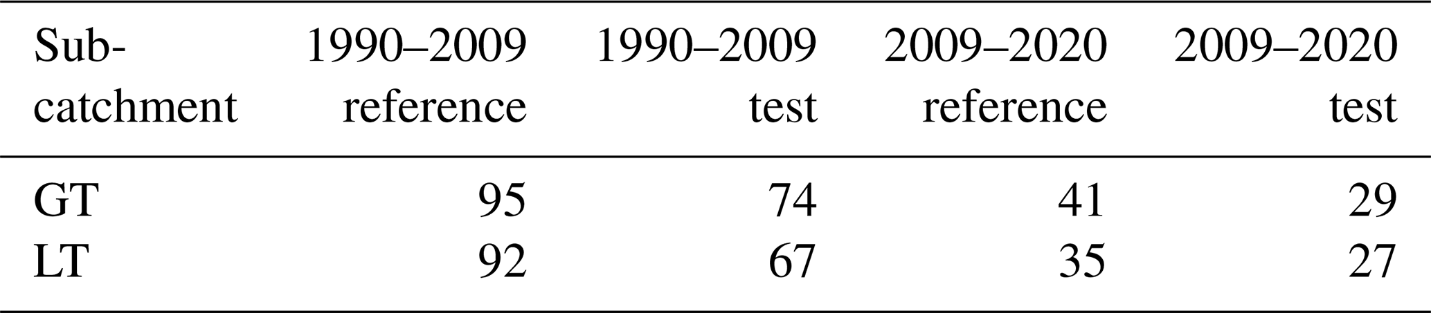
Compared to the reference data, between 22 % and 29 % of the debris flows were missed in the test mapping because of the missing orthophotos in between the timeframes. These results indicate that in longer epochs (e.g. 1954–1973) the number of slope-type debris flows is underestimated by about 25 % in relation to shorter epochs (e.g. 2015–2018) due to overlapping process areas for example.
By conducting extensive analyses on remote sensing data, we were able to detect spatial and temporal characteristics of the slope-type debris flow activity in Horlachtal. A detailed mapping using multi-temporal orthophotos revealed 834 different debris flows between 1947 and 2020. High process activity in the study area is concentrating on the west-exposed slopes of the three parallel sub-catchments GT, LT and ZT. Morphometric analyses of the hydrological catchments showed that their attributes like area, length, perimeter and relief ratio have substantial influence on the magnitude of slope-type debris flows.
From a temporal perspective, a consistent trend in frequency and magnitude since 1947 cannot be detected, as periods with enhanced debris flow activity (1954–1973, 1990–2009, 2015–2018) and periods with lower activity alternate with one another.
Spatial patterns of the mapped debris flows indicate that triggering precipitation events can occur on a very local scale. However, sub-hourly measurements of the Horlachtal meteorological station since 1989, as well as the Tschagguns station since 1953, do not show any statistical increases or decreases of days with an extreme rainfall event. For more detailed investigations on the correlations between precipitation events and slope-type debris flow activity, an extended time series with higher spatial resolution is required.
The results of this study contribute to a better understanding of slope-type debris flows in a high-alpine environment in both spatial and temporal ways, but further investigations are still necessary to better assess the process dynamics in the future. This might include an expansion of such high-resolution debris flow records e.g. using multiple methods like dendrogeomorphology or lichenometry.
Table A1Error assessment of debris flow deposit volumes between 2006 and 2019 following Anderson (2019).
Meteorological data for Horlachalm station are provided by the Tyrolean Hydropower Company (TIWAG) and are not available due to commercial restrictions. Meteorological data for Tschagguns station are provided by the Hydrographischer Dienst Vorarlberg and are available at eHYD (https://ehyd.gv.at; Hydrographischer Dienst Vorarlberg, 2023). Historical aerial images were provided by the Province of Tyrol and the Federal Office of Metrology and Surveying (BEV) and are not available due to commercial restrictions. The 2006 DEM was also provided by the Province of Tyrol and is not available due to commercial restrictions. The 2019 lidar data will be publicly available after completion of the SEHAG (SEnsitivity of High Alpine Geosystems to climate change since 1850) research project and can be provided upon request.
Planning and conceptualization were done by JR, FH and MB. JR, FH, TH, MA, FF, CR and SBN were responsible for data curation. The mapping was done by JR, and the analyses were performed by JR, MA, FF and SBN. Supervision was provided by FH, TH and MB. The original manuscript was written by JR. FH, TH, MA, FF, CR and MB were involved in reviewing and editing of the manuscript. MB, FH and TH were responsible for funding acquisition.
The contact author has declared that none of the authors has any competing interests.
Publisher’s note: Copernicus Publications remains neutral with regard to jurisdictional claims in published maps and institutional affiliations.
This study is part of the SEHAG (SEnsitivity of High Alpine Geosystems to climate change since 1850) research project, which is financially supported by the German Research Foundation (DFG), the Austrian Science Fund (FWF), the autonomous province of South Tyrol and the Swiss National Science Foundation (SNF). For providing all the essential data, we would like to thank the Tyrolean Hydropower Company (TIWAG), the Hydrographischer Dienst Vorarlberg, the Federal Office of Metrology and Surveying (BEV), and the province of Tyrol (Land Tirol). Furthermore, we want to thank the Bezirkshauptmannschaft Imst (especially Eva Loidhold and Gudrun Hofmann), the municipality of Umhausen with Jakob Wolf, as well as Johannes Kostenzer, Werner Schwarz, Kathrin Herzer and all residents of Niederthai and Umhausen, for supporting the research projects in Horlachtal. Special thanks to all the student assistants who supported our studies and to the reviewers and editors who helped to improve our manuscript.
This research has been funded by the Deutsche Forschungsgemeinschaft (DFG, German Research Foundation; project number 394200609), the Austrian Science Fund, the autonomous province of South Tyrol, and the Swiss National Science Foundation.
This paper was edited by Maria Ana Baptista and reviewed by Tjalling de Haas and one anonymous referee.
Altmann, M., Piermattei, L., Haas, F., Heckmann, T., Fleischer, F., Rom, J., Betz-Nutz, S., Knoflach, B., Müller, S., Ramskogler, K., Pfeiffer, M., Hofmeister, F., Ressl, C., and Becht, M.: Long-Term Changes of Morphodynamics on Little Ice Age Lateral Moraines and the Resulting Sediment Transfer into Mountain Streams in the Upper Kauner Valley, Austria, Water, 12, 3375, https://doi.org/10.3390/w12123375, 2020.
Anderson, S. W.: Uncertainty in quantitative analyses of topographic change: error propagation and the role of thresholding, Earth Surf. Proc. Land., 44, 1015–1033, https://doi.org/10.1002/esp.4551, 2019.
Bakker, M. and Lane, S. N.: Archival photogrammetric analysis of river-floodplain systems using Structure from Motion (SfM) methods, Earth Surf. Proc. Land., 42, 1274–1286, https://doi.org/10.1002/esp.4085, 2017.
Bates, D. M. and Watts, D. G. (Eds.): Nonlinear Regression Analysis and Its Applications, Wiley Series in Probability and Statistics, John Wiley & Sons, Inc, Hoboken, NJ, USA, https://doi.org/10.1002/9780470316757, 1988.
Baty, F., Ritz, C., Charles, S., Brutsche, M., Flandrois, J.-P., and Delignette-Muller, M.-L.: A Toolbox for Nonlinear Regression in R The Package nlstools, J. Stat. Soft., 66, 1–21, https://doi.org/10.18637/jss.v066.i05, 2015.
Bayle, A.: A recent history of deglaciation and vegetation establishment in a contrasted geomorphological context, Glacier Blanc, French Alps, J. Maps, 16, 766–775, https://doi.org/10.1080/17445647.2020.1829115, 2020.
Becht, M.: Untersuchungen zur aktuellen Reliefentwicklung in alpinen Einzugsgebieten: Mit 40 Tabellen, Zugl.: München, Univ., Habil.-Schr, Münchener Universitätsschriften/Fakultät für Geowissenschaften, 47, Geobuch-Verl., München, 187 pp., ISBN 3-925308-69-5, 1995.
Becht, M. and Rieger, D.: Debris flows on alpine slopes (eastern Alps)/Coulées de débris sur des versants des Alpes Orientales, Géomorphologie, 3, 33–41, https://doi.org/10.3406/morfo.1997.899, 1997.
Beniston, M.: Climatic Change in Mountain Regions: A Review of Possible Impacts, in: Climate Variability and Change in High Elevation Regions: Past, Present & Future, Springer, Dordrecht, 5–31, https://doi.org/10.1007/978-94-015-1252-7_2, 2003.
Beniston, M.: Mountain Climates and Climatic Change: An Overview of Processes Focusing on the European Alps, Pure Appl. Geophys., 162, 1587–1606, https://doi.org/10.1007/s00024-005-2684-9, 2005.
Bennett, G. L., Molnar, P., Eisenbeiss, H., and McArdell, B. W.: Erosional power in the Swiss Alps: characterization of slope failure in the Illgraben, Earth Surf. Proc. Land., 37, 1627–1640, https://doi.org/10.1002/esp.3263, 2012.
Berger, C., McArdell, B. W., and Schlunegger, F.: Sediment transfer patterns at the Illgraben catchment, Switzerland: Implications for the time scales of debris flow activities, Geomorphology, 125, 421–432, https://doi.org/10.1016/j.geomorph.2010.10.019, 2011.
Bernard, M., Underwood, S. J., Berti, M., Simoni, A., and Gregoretti, C.: Observations of the atmospheric electric field preceding intense rainfall events in the Dolomite Alps near Cortina d'Ampezzo, Italy, Meteorol. Atmos. Phys., 132, 99–111, https://doi.org/10.1007/s00703-019-00677-6, 2020.
Berti, M., Bernard, M., Gregoretti, C., and Simoni, A.: Physical Interpretation of Rainfall Thresholds for Runoff-Generated Debris Flows, J. Geophys. Res. Earth Surf., 125, https://doi.org/10.1029/2019JF005513, 2020.
Bollschweiler, M. and Stoffel, M.: Changes and trends in debris-flow frequency since AD 1850: Results from the Swiss Alps, Holocene, 20, 907–916, https://doi.org/10.1177/0959683610365942, 2010.
Bollschweiler, M., Stoffel, M., and Schneuwly, D. M.: Dynamics in debris-flow activity on a forested cone – A case study using different dendroecological approaches, CATENA, 72, 67–78, https://doi.org/10.1016/j.catena.2007.04.004, 2008.
Brunetti, M. T., Guzzetti, F., and Rossi, M.: Probability distributions of landslide volumes, Nonlin. Processes Geophys., 16, 179–188, https://doi.org/10.5194/npg-16-179-2009, 2009.
Chen, J.-C., Lin, C.-W., and Wang, L.-C.: Geomorphic characteristics of hillslope and channelized debris flows: A case study in the Shitou area of central Taiwan, J. Mt. Sci., 6, 266–273, https://doi.org/10.1007/s11629-009-0250-0, 2009.
Conrad, O., Bechtel, B., Bock, M., Dietrich, H., Fischer, E., Gerlitz, L., Wehberg, J., Wichmann, V., and Böhner, J.: System for Automated Geoscientific Analyses (SAGA) v. 2.1.4, Geosci. Model Dev., 8, 1991–2007, https://doi.org/10.5194/gmd-8-1991-2015, 2015.
Curry, A. M., Cleasby, V., and Zukowskyj, P.: Paraglacial response of steep, sediment-mantled slopes to post-“Little Ice Age” glacier recession in the central Swiss Alps, J. Quaternary Sci., 21, 211–225, https://doi.org/10.1002/jqs.954, 2006.
D'Agostino, V. and Marchi, L.: Debris Flows Magnitude in the Eastern Italian Alps: Data Collection and Analysis, Phys. Chem. Earth, 26, 657–663, 2001.
De Haas, T. and Densmore, A. L.: Debris-flow volume quantile prediction from catchment morphometry, Geology, 47, 791–794, https://doi.org/10.1130/G45950.1, 2019.
Dietrich, A. and Krautblatter, M.: Evidence for enhanced debris-flow activity in the Northern Calcareous Alps since the 1980s (Plansee, Austria), Geomorphology, 287, 144–158, https://doi.org/10.1016/j.geomorph.2016.01.013, 2017.
Dietrich, A. and Krautblatter, M.: Deciphering controls for debris-flow erosion derived from a LiDAR-recorded extreme event and a calibrated numerical model (Roßbichelbach, Germany), Earth Surf. Proc. Land., 44, 1346–1361, https://doi.org/10.1002/esp.4578, 2019.
Dikau, R., Eibisch, K., Eichel, J., Meßenzehl, K., and Schlummer-Held, M.: Geomorphologie, Springer Berlin Heidelberg, Berlin, Heidelberg, 487 pp., https://doi.org/10.1007/978-3-662-59402-5, 2019.
Dowling, C. A. and Santi, P. M.: Debris flows and their toll on human life: a global analysis of debris-flow fatalities from 1950 to 2011, Nat. Hazards, 71, 203–227, https://doi.org/10.1007/s11069-013-0907-4, 2014.
Fleischer, F., Haas, F., Piermattei, L., Pfeiffer, M., Heckmann, T., Altmann, M., Rom, J., Stark, M., Wimmer, M. H., Pfeifer, N., and Becht, M.: Multi-decadal (1953–2017) rock glacier kinematics analysed by high-resolution topographic data in the upper Kaunertal, Austria, The Cryosphere, 15, 5345–5369, https://doi.org/10.5194/tc-15-5345-2021, 2021.
Freeman, T.: Calculating catchment area with divergent flow based on a regular grid, Comput. Geosci., 17, 413–422, https://doi.org/10.1016/0098-3004(91)90048-I, 1991.
Gao, L., Zhang, L. M., and Cheung, R. W. M.: Relationships between natural terrain landslide magnitudes and triggering rainfall based on a large landslide inventory in Hong Kong, Landslides, 15, 727–740, https://doi.org/10.1007/s10346-017-0904-x, 2018.
Geitner, C.: Sedimentologische und vegetationsgeschichtliche Untersuchungen an fluvialen Sedimenten in den Hochlagen des Horlachtales (Stubaier Alpen/Tirol), Münchener Geographische Abhandlungen, Geobuch-Verlag, München, ISBN 3-925308-52-0, 1999.
Gillespie, C. S.: Fitting heavy tailed distributions: the poweRlaw package, J. Stat. Softw., 64, 1–16, https://doi.org/10.18637/jss.v064.i02, 2015.
Glira, P., Pfeifer, N., Briese, C., and Ressl, C.: RIGOROUS STRIP ADJUSTMENT OF AIRBORNE LASERSCANNING DATA BASED ON THE ICP ALGORITHM, ISPRS Ann. Photogramm. Remote Sens. Spatial Inf. Sci., II-3/W5, 73–80, https://doi.org/10.5194/isprsannals-II-3-W5-73-2015, 2015.
Glira, P., Pfeifer, N., and Mandlburger, G.: Rigorous Strip Adjustment of UAV-based Laserscanning Data Including Time-Dependent Correction of Trajectory Errors, Photogram. Engng. Rem. Sens., 82, 945–954, https://doi.org/10.14358/PERS.82.12.945, 2016.
Griswold, J. P. and Iverson, R. M.: Mobility Statistics and Automated Hazard Mapping for Debris Flows and Rock Avalanches, Scientific Investigations Report 2007–5276, US Geological Survey, https://doi.org/10.3133/sir20075276, 2008.
Guzzetti, F., Ardizzone, F., Cardinali, M., Rossi, M., and Valigi, D.: Landslide volumes and landslide mobilization rates in Umbria, central Italy, Earth Planet. Sc. Lett., 279, 222–229, https://doi.org/10.1016/j.epsl.2009.01.005, 2009.
Haas, F., Heckmann, T., Wichmann, V., and Becht, M.: Runout analysis of a large rockfall in the Dolomites/Italian Alps using LIDAR derived particle sizes and shapes, Earth Surf. Proc. Land., 37, 1444–1455, https://doi.org/10.1002/esp.3295, 2012.
Heckmann, T. and Schwanghart, W.: Geomorphic coupling and sediment connectivity in an alpine catchment — Exploring sediment cascades using graph theory, Geomorphology, 182, 89–103, https://doi.org/10.1016/j.geomorph.2012.10.033, 2013.
Heckmann, T., Haas, F., Morche, D., Schmidt, K., Rohn, J., Moser, M., Leopold, M., Kuhn, M., Briese, C., Pfeifer, N., and Becht, M.: Investigating an Alpine proglacial sediment budget using field measurements, airborne and terrestrial LiDAR data, IAHS-AISH P., 356, 438–447, 2012.
Heckmann, T., Gegg, K., Gegg, A., and Becht, M.: Sample size matters: investigating the effect of sample size on a logistic regression susceptibility model for debris flows, Nat. Hazards Earth Syst. Sci., 14, 259–278, https://doi.org/10.5194/nhess-14-259-2014, 2014.
Helsen, M. M., Koop, P. J. M., and van Steijn, H.: Magnitude-frequency relationship for debris flows on the fan of the Chalance torrent, Valgaudemar (French Alps), Earth Surf. Proc. Land., 27, 1299–1307, https://doi.org/10.1002/esp.412, 2002.
Hilger, L.: Quantification and regionalization of geomorphic processes using spatial models and high-resolution topographic data: A sediment budget of the Upper Kauner Valley, Ötztal Alps, PhD thesis, Katholische Universität Eichstätt-Ingolstadt, Eichstätt-Ingolstadt, URN urn:nbn:de:bvb:824-opus4-3814, 2017.
Hirschberg, J., Fatichi, S., Bennett, G. L., McArdell, B. W., Peleg, N., Lane, S. N., Schlunegger, F., and Molnar, P.: Climate Change Impacts on Sediment Yield and Debris-Flow Activity in an Alpine Catchment, J. Geophys. Res.-Earth, 126, e2020JF005739, https://doi.org/10.1029/2020JF005739, 2021.
Hungr, O., McDougall, S., Wise, M., and Cullen, M.: Magnitude-frequency relationships of debris flows and debris avalanches in relation to slope relief, Geomorphology, 96, 355–365, https://doi.org/10.1016/j.geomorph.2007.03.020, 2008.
Hydrographischer Dienst Vorarlberg: Meteorological data for Tschagguns station, eHYD [data set], https://ehyd.gv.at, last access: 7 February 2023.
Innes, J. L.: Lichenometric dating of debris-flow deposits in the Scottish Highlands, Earth Surf. Proc. Land., 8, 579–588, https://doi.org/10.1002/esp.3290080609, 1983.
Iverson, R. M.: Elementary theory of bed-sediment entrainment by debris flows and avalanches, J. Geophys. Res., 117, F03006, https://doi.org/10.1029/2011JF002189, 2012.
Jaboyedoff, M., Carrea, D., Derron, M.-H., Oppikofer, T., Penna, I. M., and Rudaz, B.: A review of methods used to estimate initial landslide failure surface depths and volumes, Eng. Geol., 267, 105478, https://doi.org/10.1016/j.enggeo.2020.105478, 2020.
Jakob, M., Bovis, M., and Oden, M.: The significance of channel recharge rates for estimating debris-flow magnitude and frequency, Earth Surf. Proc. Land., 30, 755–766, https://doi.org/10.1002/esp.1188, 2005.
Jakob, M., Mark, E., McDougall, S., Friele, P., Lau, C.-A., and Bale, S.: Regional debris-flow and debris-flood frequency–magnitude relationships, Earth Surf. Proc. Land., 45, 2954–2964, https://doi.org/10.1002/esp.4942, 2020.
Jomelli, V., Brunstein, D., Chochillon, C., and Pech, P.: Hillslope debris-flow frequency since the beginning of the 20th century in the Massif des Ecrins (French Alps), in: Debris-Flow Hazards Mitigation: Mechanics, Prediction, and Assessment, edited by: Rickenmann, D. and Chen, C., Millpress, Rotterdam, 127–137, ISBN 978-90-77017-78-4, 2003.
Jomelli, V., Grancher, D., Naveau, P., Cooley, D., and Brunstein, D.: Assessment study of lichenometric methods for dating surfaces, Geomorphology, 86, 131–143, https://doi.org/10.1016/j.geomorph.2006.08.010, 2007.
Kiefer, C., Oswald, P., Moernaut, J., Fabbri, S. C., Mayr, C., Strasser, M., and Krautblatter, M.: A 4000-year debris flow record based on amphibious investigations of fan delta activity in Plansee (Austria, Eastern Alps), Earth Surf. Dynam., 9, 1481–1503, https://doi.org/10.5194/esurf-9-1481-2021, 2021.
Lane, S. N., Westaway, R. M., and Murray Hicks, D.: Estimation of erosion and deposition volumes in a large, gravel-bed, braided river using synoptic remote sensing, Earth Surf. Proc. Land., 28, 249–271, https://doi.org/10.1002/esp.483, 2003.
Larsen, I. J., Montgomery, D. R., and Korup, O.: Landslide erosion controlled by hillslope material, Nat. Geosci., 3, 247–251, https://doi.org/10.1038/ngeo776, 2010.
Li, L., Yu, B., Zhu, Y., Chu, S., and Wu, Y.: Topographical factors in the formation of gully-type debris flows in Longxi River catchment, Sichuan, China, Environ. Earth Sci., 73, 4385–4398, https://doi.org/10.1007/s12665-014-3722-7, 2015.
Lopez Saez, J., Corona, C., Stoffel, M., Gotteland, A., Berger, F., and Liébault, F.: Debris-flow activity in abandoned channels of the Manival torrent reconstructed with LiDAR and tree-ring data, Nat. Hazards Earth Syst. Sci., 11, 1247–1257, https://doi.org/10.5194/nhess-11-1247-2011, 2011.
Magirl, C. S., Griffiths, P. G., and Webb, R. H.: Analyzing debris flows with the statistically calibrated empirical model LAHARZ in southeastern Arizona, USA, Geomorphology, 119, 111–124, https://doi.org/10.1016/j.geomorph.2010.02.022, 2010.
Marchi, L. and Tecca, P. R.: Some Observations on the Use of Data from Historical Documents in Debris-Flow Studies, Nat. Hazards, 38, 301–320, https://doi.org/10.1007/s11069-005-0264-z, 2006.
Marchi, L., Brunetti, M. T., Cavalli, M., and Crema, S.: Debris-flow volumes in northeastern Italy: Relationship with drainage area and size probability, Earth Surf. Proc. Land., 44, 933–943, https://doi.org/10.1002/esp.4546, 2019.
McGlone, J. C., Mikhail, E., and Bethel, J. (Eds.): Manual of Photogrammetry, 5th edn., ASPRS American Soc. for Photogrammetry and Remote Sensing, Bethesda, Md., ISBN 1570830711, 2004.
Melton, M.: An analysis of the relations among elements of climate, surface properties, and geomorphology, Technical Report No. 11, Department of Geology, Columbia University, New York, https://doi.org/10.21236/ad0148373, 1957.
Nogués-Bravo, D., Araújo, M. B., Errea, M. P., and Martínez-Rica, J. P.: Exposure of global mountain systems to climate warming during the 21st Century, Global Environ. Chang., 17, 420–428, https://doi.org/10.1016/j.gloenvcha.2006.11.007, 2007.
Nuth, C. and Kääb, A.: Co-registration and bias corrections of satellite elevation data sets for quantifying glacier thickness change, The Cryosphere, 5, 271–290, https://doi.org/10.5194/tc-5-271-2011, 2011.
Pelfini, M. and Santilli, M.: Frequency of debris flows and their relation with precipitation: A case study in the Central Alps, Italy, Geomorphology, 101, 721–730, https://doi.org/10.1016/j.geomorph.2008.04.002, 2008.
Petrini-Monteferri, F., Wichmann, V., Georges, C., Mantovani, D., and Stötter, J.: Erweiterung der GIS Software SAGA zur Verarbeitung von Laserscanning-Daten der Autonomen Provinz Bozen-Südtirol, in: Angewandte Geoinformatik 2009: Beiträge zum 21. AGIT-Symposium Salzburg, edited by: Strobl, J. and Blaschke, T., Wichmann, Heidelberg, 47–52, ISBN 3879074801, 2009.
Pfeifer, N., Mandlburger, G., Otepka, J., and Karel, W.: OPALS – A framework for Airborne Laser Scanning data analysis, Comput. Environ. Urban, 45, 125–136, https://doi.org/10.1016/j.compenvurbsys.2013.11.002, 2014.
Rainato, R., Mao, L., García-Rama, A., Picco, L., Cesca, M., Vianello, A., Preciso, E., Scussel, G. R., and Lenzi, M. A.: Three decades of monitoring in the Rio Cordon instrumented basin: Sediment budget and temporal trend of sediment yield, Geomorphology, 291, 45–56, https://doi.org/10.1016/j.geomorph.2016.03.012, 2017.
Ravanel, L. and Deline, P.: Climate influence on rockfalls in high-Alpine steep rockwalls: The north side of the Aiguilles de Chamonix (Mont Blanc massif) since the end of the “Little Ice Age”, Holocene, 21, 357–365, https://doi.org/10.1177/0959683610374887, 2011.
Rickenmann, D. and Zimmermann, M.: The 1987 debris flows in Switzerland: documentation and analysis, Geomorphology, 8, 175–189, https://doi.org/10.1016/0169-555X(93)90036-2, 1993.
Rieger, D.: Bewertung der naturräumlichen Rahmenbedingungen für die Entstehung von Hangmuren: Möglichkeiten zur Modellierung des Murpotentials; mit 21 Tabellen, Zugl.: München, Univ., Diss., 1998, Münchener Universitätsschriften/Fakultät für Geowissenschaften, 51, Geobuch-Verl., München, 149 pp., ISBN 3925308733, 1999.
Riley, K. L., Bendick, R., Hyde, K. D., and Gabet, E. J.: Frequency–magnitude distribution of debris flows compiled from global data, and comparison with post-fire debris flows in the western U.S., Geomorphology, 191, 118–128, https://doi.org/10.1016/j.geomorph.2013.03.008, 2013.
Rom, J., Haas, F., Stark, M., Dremel, F., Becht, M., Kopetzky, K., Schwall, C., Wimmer, M., Pfeifer, N., Mardini, M., and Genz, H.: Between Land and Sea: An Airborne LiDAR Field Survey to Detect Ancient Sites in the Chekka Region/Lebanon Using Spatial Analyses, Open Archaeology, 6, 248–268, https://doi.org/10.1515/opar-2020-0113, 2020.
Sassa, K.: The mechanism to initiate debris flows as undrained shear of loose sediments, Internationales Symposion Interpraevent – Villach Tagespublikation, 2, 73–87, http://www.interpraevent.at/palm-cms/upload_files/Publikationen/Tagungsbeitraege/1984_2_73.pdf (last access: 6 February 2023), 1984.
Segoni, S., Piciullo, L., and Gariano, S. L.: A review of the recent literature on rainfall thresholds for landslide occurrence, Landslides, 15, 1483–1501, https://doi.org/10.1007/s10346-018-0966-4, 2018.
Shen, C.-W., Lo, W.-C., and Chen, C.-Y.: Evaluating Susceptibility of Debris Flow Hazard using Multivariate Statistical Analysis in Hualien County, Disaser Advances, vol. 5, http://hdl.handle.net/11536/20889 (last access: 6 February 2023), 2012.
Spiess, A.-N. and Neumeyer, N.: An evaluation of R2 as an inadequate measure for nonlinear models in pharmacological and biochemical research: a Monte Carlo approach, BMC Pharmacol., 10, 6, https://doi.org/10.1186/1471-2210-10-6, 2010.
Stoffel, M.: Magnitude–frequency relationships of debris flows – A case study based on field surveys and tree-ring records, Geomorphology, 116, 67–76, https://doi.org/10.1016/j.geomorph.2009.10.009, 2010.
Stoffel, M., Lièvre, I., Conus, D., Grichting, M. A., Raetzo, H., Gärtner, H. W., and Monbaron, M.: 400 Years of Debris-Flow Activity and Triggering Weather Conditions: Ritigraben, Valais, Switzerland, Arct. Antarct. Alp. Res., 37, 387–395, https://doi.org/10.1657/1523-0430(2005)037[0387:YODAAT]2.0.CO;2, 2005.
Stoffel, M., Mendlik, T., Schneuwly-Bollschweiler, M., and Gobiet, A.: Possible impacts of climate change on debris-flow activity in the Swiss Alps, Climatic Change, 122, 141–155, https://doi.org/10.1007/s10584-013-0993-z, 2014.
Tanyaş, H., Westen, C. J., Allstadt, K. E., and Jibson, R. W.: Factors controlling landslide frequency–area distributions, Earth Surf. Proc. Land., 44, 900–917, https://doi.org/10.1002/esp.4543, 2019.
Theule, J. I., Liébault, F., Loye, A., Laigle, D., and Jaboyedoff, M.: Sediment budget monitoring of debris-flow and bedload transport in the Manival Torrent, SE France, Nat. Hazards Earth Syst. Sci., 12, 731–749, https://doi.org/10.5194/nhess-12-731-2012, 2012.
Thiel, M.: Quantifizierung der Konnektivität von Sedimentkaskaden in alpinen Geosystemen, PhD thesis, Katholische Universität Eichstätt-Ingolstadt, Eichstätt-Ingolstadt, 186 pp., URN urn:nbn:de:bvb:824-opus4-1081, 2013.
Tropeano, D. and Turconi, L.: Using Historical Documents for Landslide, Debris Flow and Stream Flood Prevention. Applications in Northern Italy, Nat. Hazards, 31, 663–679, https://doi.org/10.1023/B:NHAZ.0000024897.71471.f2, 2004.
Turnbull, B., Bowman, E. T., and McElwaine, J. N.: Debris flows: Experiments and modelling, C. R. Phys., 16, 86–96, https://doi.org/10.1016/j.crhy.2014.11.006, 2015.
Underwood, S. J., Schultz, M. D., Berti, M., Gregoretti, C., Simoni, A., Mote, T. L., and Saylor, A. M.: Atmospheric circulation patterns, cloud-to-ground lightning, and locally intense convective rainfall associated with debris flow initiation in the Dolomite Alps of northeastern Italy, Nat. Hazards Earth Syst. Sci., 16, 509–528, https://doi.org/10.5194/nhess-16-509-2016, 2016.
Varnes, D. J.: Slope Movement Types and Processes, in: Landslides, analysis and control (Special report-Transportation Research Board), edited by: Schuster, R. L. and Krizek, R. J., National Academy of Sciences, Washington, DC, 11–33, ISBN 9780309028042, 1978.
Wichmann, V.: Modellierung geomorphologischer Prozesse in einem alpinen Einzugsgebiet: Abgrenzung und Klassifizierung der Wirkungsräume von Sturzprozessen und Muren mit einem GIS, Zugl.: Eichstätt, Katholische Univ., Diss., 2005 u.d.T.: Wichmann, Volker: Entwicklung von prozessorientierten Modellen zur flächenverteilten Abgrenzung und Klassifizierung der Wirkungsräume von Sturzprozessen und Muren mit einem GIS – dargestellt am Einzugsgebiet des Lahnenwiesgrabens Ammergebirge, Eichstätter Geographische Arbeiten, 15, Profil-Verl., München, Wien, 231 pp., ISBN 3-89019-605-5, 2006.
Wichmann, V.: The Gravitational Process Path (GPP) model (v1.0) – a GIS-based simulation framework for gravitational processes, Geosci. Model Dev., 10, 3309–3327, https://doi.org/10.5194/gmd-10-3309-2017, 2017.
Wilford, D. J., Sakals, M. E., Innes, J. L., Sidle, R. C., and Bergerud, W. A.: Recognition of debris flow, debris flood and flood hazard through watershed morphometrics, Landslides, 1, 61–66, https://doi.org/10.1007/s10346-003-0002-0, 2004.
Winter, M. G.: Debris flows, in: Geological hazards in the UK: Their occurrence, monitoring and mitigation Engineering Group working party report, edited by: Giles, D. P. and Griffiths, J. S., The Geological Society, London, 163–185, https://doi.org/10.1144/EGSP29.5, 2020.
Wu, W.: Recent Advances in Modeling Landslides and Debris Flows, Springer International Publishing, Cham, Heidelberg, New York, Dordrecht, London, 318 pp., ISBN 978-3-319-11052-3, 2015.
Zhao, Y., Meng, X., Qi, T., Qing, F., Xiong, M., Li, Y., Guo, P., and Chen, G.: AI-based identification of low-frequency debris flow catchments in the Bailong River basin, China, Geomorphology, 359, 107125, https://doi.org/10.1016/j.geomorph.2020.107125, 2020.
Zhou, W., Tang, C., van Asch, T. W. J., and Chang, M.: A rapid method to identify the potential of debris flow development induced by rainfall in the catchments of the Wenchuan earthquake area, Landslides, 13, 1243–1259, https://doi.org/10.1007/s10346-015-0631-0, 2016.
Zimmermann, M.: Debris flows 1987 in Switzerland: geomorphological and meteorological aspects, IAHS, Hydrol. Mountainous Regions, 2, 387–393, https://iahs.info/uploads/dms/iahs_194_0387.pdf (last access: 6 February 2023), 1990.