Bare-earth DEM generation from ArcticDEM and its use in flood simulation

In urban areas, topography data without above-ground objects are typically preferred in wide-area flood simulation but are not yet available for many locations globally. High-resolution satellite photogrammetric DEMs, like ArcticDEM, are now emerging and could prove extremely useful for global urban flood modelling; however, approaches to generate bare-earth DEMs from them have not yet been fully investigated. In this paper, we test the use of two morphological filters (simple morphological filter – SMRF – and progressive morphological filter – PMF) to remove surface artefacts from ArcticDEM using the city of Helsinki (192 km²) as a case study. The optimal filter is selected and used to generate a bare-earth version of ArcticDEM. Using a lidar digital terrain model (DTM) as a benchmark, the elevation error and flooding simulation performance for a pluvial scenario were then evaluated at 2 and 10 m spatial resolution, respectively. The SMRF was found to be more effective at removing artefacts than PMF over a broad parameter range. For the optimal ArcticDEM-SMRF the elevation RMSE was reduced by up to 70 % over the uncorrected DEM, achieving a final value of 1.02 m. The simulated water depth error was reduced to 0.3 m, which is comparable to typical model errors using lidar DTM data. This paper indicates that the SMRF can be directly applied to generate a bare-earth version of ArcticDEM in urban environments, although caution should be exercised for areas with densely packed buildings or vegetation. The results imply that where lidar DTMs do not exist, widely available high-resolution satellite photogrammetric DEMs could be used instead.

1 Introduction

The availability of an accurate bare-earth digital elevation model (DEM) is important to many research fields, including identifying drainage-related features and modelling flood inundation (Garbrecht and Martz, 2000; Yamazaki et al., 2014), deriving topography indices such as slope, orientation, and rugosity (Moudrý et al., 2018), estimating forest biomass and carbon (Jensen and Mathews, 2016), and constructing 3D building heights (Marconcini et al., 2014). For wide-area flood simulation in urban areas, a bare-earth DEM (i.e. a terrain model without surface artefacts) is preferable in most circumstances to a digital surface model (DSM) which includes them. This is because the decision to include above-terrain artefacts or not is a consequence of the selected simulation resolution. Only when the simulation is conducted at grid sizes allowing the resolution of building shapes and the street layout (typically < 5 m in most urban topologies worldwide) does a DSM become useful. When aggregated to coarser resolutions, the height of the surface artefacts contained in the DSM can block or alter flow pathways in ways that lead to anomalous results when these data are used in hydrodynamic modelling (Neal et al., 2009). Inundation simulations over regional and national scales usually only become feasible with non-building-resolving grid resolutions because of the disproportionally increased computational cost of running fine grid models (roughly a factor of 3 to the grid change) and the limited availability of national DEMs with resolutions finer than 5 m. Even at city and sub-city scales, non-building-resolving models may be preferable for ensemble and event set simulations (Mason et al., 2007; Schubert and Sanders, 2012). As a result, bare-earth DEMs (also known as digital terrain models or DTMs) are essential for flood inundation simulations in urban areas and can also be beneficial to a broad range of other research fields.

Unlike traditional, ground-based field surveys, modern wide-area DEM collection techniques rely on remote sensing from ground vehicle, airborne, and satellite platforms. All DEMs derived in this way include the heights of built-up area artefacts and vegetation to some extent and require significant post-processing to obtain a bare-earth DEM. Commonly used DEMs are collected using techniques including interferometric synthetic aperture radar (i.e. InSAR), optical stereo mapping, and lidar. These different techniques, combined with the platforms and the specific instrument characteristics, offer DEMs with varied coverage, resolution, and accuracy (Lakshmi and Yarrakula, 2018; Zaidi et al., 2018). For example, spaceborne and globally available InSAR DEMs offer wide coverage, but they are constrained by the geometry of the interferometric baseline and the temporal sampling of the spaceborne platform and InSAR technique. The derived DEMs therefore have limited horizontal resolution and accuracy (Shuttle Radar Topography Mission – SRTM – at ∼ 30 m spatial resolution has reported mean absolute vertical error of 6 m, and TanDEM-X at ∼ 12 m spatial resolution has 90 % linear error (i.e. LE90) in the vertical of around 2 m) (Rodriguez et al., 2006; Wessel et al., 2018). Such vertical errors are significant compared to the amplitude of most river flood waves, which typically range from 1–2 m up to ∼ 12 m for the Amazon River at Manaus in Brazil (Trigg et al., 2009; Bates et al., 2013). Whilst global InSAR DEM errors can be reduced by intelligent processing (O'Loughlin et al., 2016; Yamazaki et al., 2017; Archer et al., 2018; Liu et al., 2021; Hawker et al., 2022) and by aggregating to coarser grid resolutions to mitigate random errors, they remain distinctly sub-optimal for a lot of flood inundation modelling (Schumann and Bates, 2018). Instead, inundation modelling is best conducted with DEMs generated using airborne lidars for most applications. These have high accuracy, with a typical vertical RMSE of 0.05–0.2 m (Faherty et al., 2020) and spatial resolution of 1–2 m such that they can identify the detailed structure of floodplain geomorphology, buildings, vegetation, and important linear features such as flood defences and their crest elevations. However, due to their (relatively) high cost of collection, freely available lidar data only cover ∼ 0.005 % of the global land surface (Hawker et al., 2018). DEMs derived from high-resolution stereo images, such as WorldView, have the potential to cover the land surface globally with spatial resolution (and also perhaps accuracy) comparable to lidar (Noh and Howat, 2015; Hu et al., 2016; Shean et al., 2016; DeWitt et al., 2017). Whilst stereo photogrammetry was previously used to develop the publicly available AW3D30 DEM (Takaku et al., 2016), the DEM developed at the original resolution of 5 m (AW3D30) has been kept as a commercial product. DEMs derived from other high-resolution photogrammetric satellites such as WorldView, GeoEye, IKONOS, and Pleiades are also only available with a cost that is prohibitive for most academic studies. However, the recent public release of a satellite photogrammetric DEM at an unprecedented resolution (2 m), ArcticDEM (Porter et al., 2018, https://www.pgc.umn.edu/data/arcticdem/, last access: 26 January 2023), has brought opportunities to explore the potential of such a product in flood inundation modelling. ArcticDEM covers areas above 60^∘ N and was produced using the surface extraction with TIN-based search-space minimization (SETSM) method from in-track and cross-track high-resolution (∼ 0.5 m) imagery acquired by the WorldView and GeoEye satellites. Using similar stereo-photogrammetric techniques, Google is also developing a very high-resolution DEM using multiple satellite sources (Ben-Haim et al., 2019). However, both products are DSMs and therefore contain surface artefacts which need to be removed to enable their use in a range of geophysics applications including wide-area flood inundation modelling. Previous research efforts to generate bare-earth terrain data from previously released global DEMs such as SRTM and TanDEM-X have relied heavily on auxiliary data to remove artefacts. For these next generation of high-resolution photogrammetric DEMs, auxiliary data at comparable resolution to the DEM do not yet exist, and different approaches must be proposed.

Considering the high resolution of these photogrammetric DEMs, the algorithms already developed to create bare-earth DEMs from lidar are likely to be applicable to this task. For example, DeWitt et al. (2017) have shown that applying lidar filtering procedures to a WorldView-generated DEM in densely vegetated areas can remove vegetation artefacts and achieve a bare-earth terrain representation with accuracy comparable to lidar. Numerous research studies have been conducted in the past decade to generate bare-earth DEMs (i.e. DTMs) from lidar point clouds (Sithole and Vosselman, 2004; Chen et al., 2007; Meng et al., 2009; Zhang et al., 2016). Filtering strategies were reviewed by Chen et al. (2017), and morphology-based filters were reported as robust and capable of removing non-ground objects. Notably, Zhang et al. (2003) proposed a progressive morphological filter (PMF) for removing non-ground measurements from airborne lidar. The PMF method subsequently advanced previous methods by enabling automatic extraction of ground points from lidar measurements with minimal human interaction and is now widely used as a base filter to classify ground and non-ground points (Cui et al., 2013; Hui et al., 2016; Tan et al., 2018). Evolved from the morphological filter idea, Pingel et al. (2013) developed the simple morphological filter (SMRF) by designating the window size increasement strategy of the filter and employing a computationally inexpensive technique to interpolate the non-ground pixels. The SMRF was reportedly able to achieve low misclassification errors (2.97 %) among 11 filter algorithms for lidar DEM samples with various configurations of slope and artefacts and to be robust with respect to the algorithm parameterization (Zhang et al., 2016). However, despite previous research applying lidar filtering strategies to WorldView photogrammetric DEMs (Rokhmana and Sastra, 2020), none of these filters has been tested on ArcticDEM, and research about the performance of different filters for removing surface artefacts from high-resolution photogrammetric DSMs is also lacking, especially in urban areas.

Given their unprecedented resolution and potential wide-area coverage, bare-earth photogrammetric DEMs can possibly be used to advance flood inundation simulations at regional scales and beyond. Although at this stage the access to these DEMs is restricted, they are very promising and could become an alternative to lidar data in the future as a result of their much lower cost. This could especially benefit developing countries where wide coverage of lidar data is likely to prove unaffordable for the foreseeable future. This research therefore aims to develop an approach to generate bare-earth DEMs from ArcticDEM and to examine the use of the data in flood inundation simulation. The proposed approach is expected to be generally applicable to other high-resolution (∼ m scale) photogrammetric DEMs, as well as ArcticDEM. We first compare the ability of progressive and simple morphological filters (PMF and SMRF) to generate a bare-earth DEM from ArcticDEM in the city of Helsinki, Finland, by evaluating the filtered ArcticDEMs against a reference bare-earth lidar data set. Next, for the best-performing filter a set of parameter combinations was applied to generate a realization ensemble of filtered ArcticDEM, whose error metrics were then analysed against the parameter settings. We then use both the original ArcticDEM and filtered ArcticDEM realizations to simulate a pluvial flooding scenario for Helsinki and compare these results to an identical simulation using the lidar DTM. Pluvial flood simulation is difficult for hydrodynamic models even with excellent terrain data and therefore poses a rigorous and diagnostic test. Lastly, limitations of the current research and future work that could further facilitate the use of a bare-earth version of ArcticDEM in flood inundation simulation are discussed.

2 Data source and study site

ArcticDEM is stereo-photogrammetric DSM generated from in-track and cross-track high-resolution (∼ 0.5 m) imagery acquired by the DigitalGlobe constellation of optical imaging satellites. The majority of ArcticDEM data was generated from the panchromatic bands of the WorldView-1, WorldView-2, and WorldView-3 satellites. A small percentage of data was also sourced from the GeoEye-1 satellite sensor. ArcticDEM is available in two formats: strip and mosaic. Strip data are the output extracted by the TIN-based search-space minimization algorithm (Noh and Howat, 2015) and preserve the original source material temporal resolution. Mosaic data are compiled from multiple strips that have been co-registered, blended, and feathered to reduce edge-matching artefacts. Due to the errors in the sensor model, the geolocation of the generated ArcticDEM has systematic offsets in the vertical and horizontal directions which are reported in the product's meta-data. Offsets for the mosaic data are unknown, so therefore the strip data set with the original horizontal resolution at 2 m (version 3.0) was used as the baseline DEM in this paper. The offset values of each strip data were applied before generating the bare-earth ArcticDEM.

The city of Helsinki was selected as a study site for the following reasons: (1) both ArcticDEM and a high-accuracy lidar DTM are available at this site; (2) it is a typical urban environment with sparse to medium-density buildings mixed with large patches of vegetation; and (3) as the most populated city above 60^∘ N, the Helsinki metropolitan area is very vulnerable to flooding. The lidar DTM has a spatial resolution of 2 m and a reported vertical error of 0.3 m (National Land Survey of Finland, 2017a, b). To standardize the vertical reference system, the quasi-geoid height was subtracted from ArcticDEM, converting its reference system from WGS84 ellipsoid height to the Finland National Vertical Reference N2000 that is used for the lidar data. This conversion has an accuracy of 0.02 m (National Land Survey of Finland, 2005).

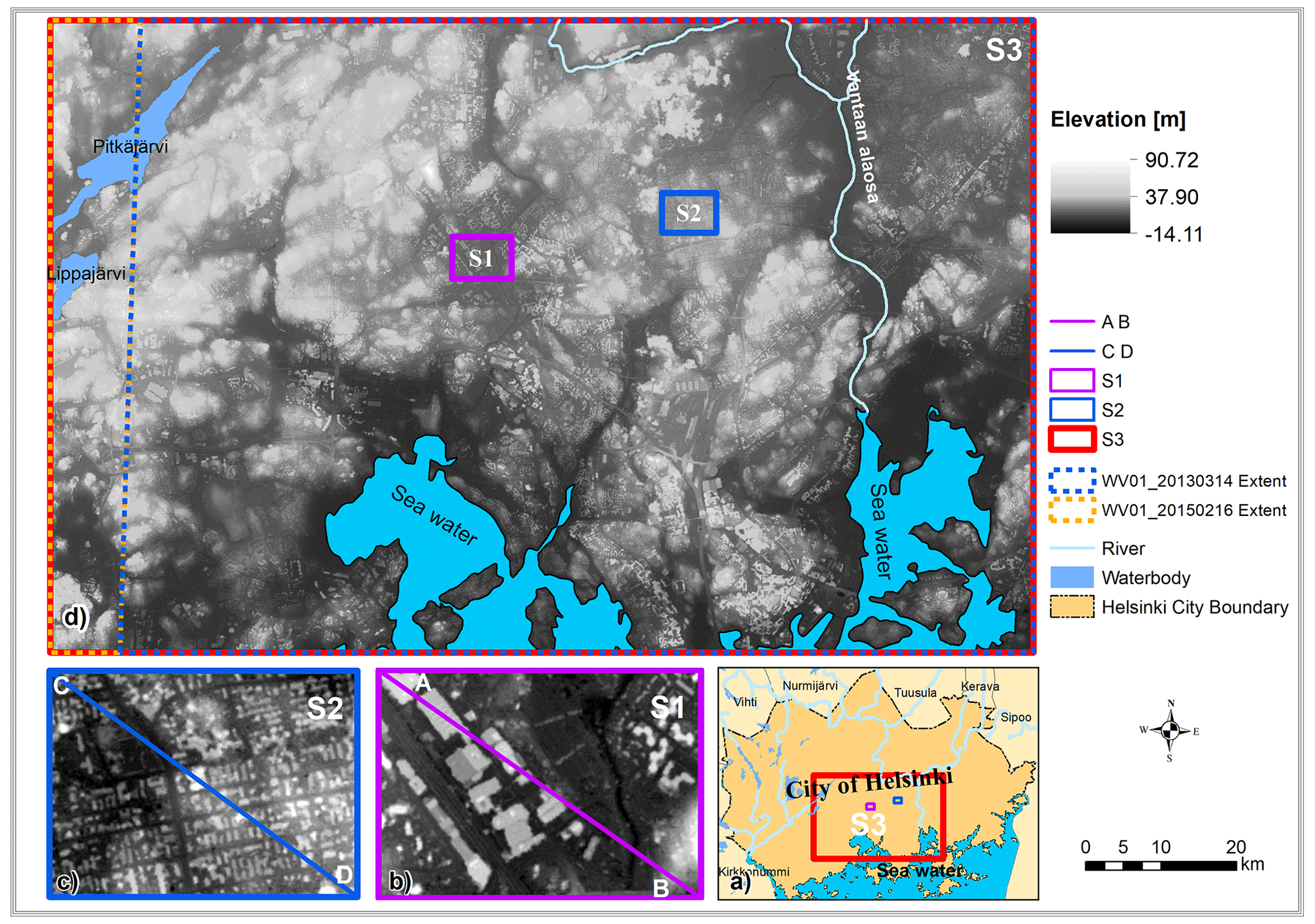
Figure 1 Locations of the three studied samples (S1, S2, and S3) within the city of Helsinki are shown in (a). Elevation values of the ArcticDEM at S1, S2 (overlain with transects crossing), and S3 are shown in (b–d), respectively. Locations of coastal areas, lakes, and rivers are also labelled. The ArcticDEM strip data are acquired from the Polar Geospatial Center at https://data.pgc.umn.edu/elev/dem/setsm/ArcticDEM/mosaic/v3.0/2m/ (last access: 26 January 2023). The waterbody outlines were acquired from the Finnish Environment Institute at https://wwwd3.ymparisto.fi/d3/gis_data/spesific/VHSvesimuodostumat2016.zip (last access: 26 January 2023).

Within the city of Helsinki two building-dominated samples (S1 and S2, both covering areas of ∼ 0.7 km²) were chosen to compare the effectiveness of two selected morphological filters: the PMF and the SMRF. Sample 1 is characterized by buildings with floor areas up to 10 000 m², whereas smaller buildings (floor areas of ∼ 500 m²) are distributed throughout sample 2. A larger third sample (S3, which includes both S1 and S2) was selected to conduct the bare-earth DEM generation and to assess the filter's performance in a complex urban environment. Flood inundation performance of the resulting DEM data was also evaluated over sample area S3 (Fig. 1). The ArcticDEM strip data derived from WorldView-1 images acquired on 14 March 2013 (WV01_20130314) and on 16 February 2015 (WV01_20150216) were found to cover most areas of S3 (92 % and 99 %, respectively). Considering the possible bias caused by forest and snow, the ArcticDEM strips with source images acquired during leaf-off seasons and under snow-free conditions are preferable. Finnish forests are reported to be mostly evergreen with ∼ 10 % deciduous trees (Majasalmi and Rautiainen, 2021). The source images of both strips were acquired during leaf-off conditions. The snow situation on the image acquisition dates was analysed using the MODIS NDSI_Snow Cover data (Hall and Riggs, 2016). The acquisition date of strip WV01_20130314 was found to be much less covered by snow compared to that of strip WV01_20150216. Therefore, strip WV01_20130314 was used as the main data source, and areas within S3 which this strip does not cover or where voids were present were filled with data from strip WV01_20150216. These mosaicked strip data are shown in Fig. 1, with the extent of the two strips displayed. The ArcticDEM for all samples in this paper refers to this mosaicked data set. Land use and land cover (LULC) for Helsinki were acquired from the CORINE Urban Atlas 2012 database (https://land.copernicus.eu/local/urban-atlas/urban-atlas-2012, last access: 26 January 2023). This LULC features 22 land cover types in Helsinki. In this paper, features were merged to four categories: urban, forest, open land, and water. Details of this reclassification of the LULC data can be found in Table S1 in the Supplement.

3 Methods

3.1 Morphological filters

The generation of bare-earth ArcticDEM (our version of ArcticDEM with artefacts removed) was conducted by employing two different morphological filters: PMF and SMRF separately. They are considered because of their reported effectiveness in filtering lidar point clouds, simple conceptualized parameters, and the fact that they are open access.

The PMF was designed to remove non-ground measurements (buildings, vegetation, vehicles) from airborne lidar data (Zhang et al., 2003). It consists of an object detection and an interpolation process which employs non-object pixel elevations to generate the values of the object pixels. The PMF provides an advance on the morphological filter algorithm (Kilian et al., 1996) by enabling a gradually increasing window width to detect non-ground objects regardless of their size. In addition, an elevation difference threshold based on elevation variations in the terrain, buildings, and trees was introduced to preserve the terrain. The maximum window size and elevation variation threshold parameters control the filtering process (more details can be found at Zhang et al., 2003).

More recently, a SMRF was proposed by Pingel et al. (2013), also with the aim of removing non-ground measurements from airborne lidar data. While the SMRF follows a similar two-step process to the PMF, the approaches taken to detect objects and interpolate elevation values of objects are different. SMRF adopts a linearly increasing window (as opposed to the exponential increase in PMF) and simple slope thresholding, along with a novel image inpainting technique. Like the PMF, the maximum window size (W_max) and slope threshold (S) (equivalent to the elevation variation threshold of PMF) parameters control the performance of the filter (Fig. 2). The core of the filter is the object detection where morphological opening is applied to the original surface based on the current window size (W_i) increasing from 1 pixel, by 1 pixel, to the maximum window size (in distance units, metres in this research). For each window size within the range, the difference between the original surface (W_i = 1) or the surface from the last step (W_i > 1) and the morphologically opened surface is calculated, and this difference (for example, d₀, d₁, d₂ in Fig. 2) is compared with the current difference threshold (D_i) (defined as the slope threshold S multiplied by the current window size W_i) to determine whether the object flag of the pixel should be accepted or rejected. When the difference is smaller than the current difference threshold (D_i), the object flag of these pixels is rejected (Fig. 2III), and the elevated areas are retained. Otherwise, pixels are flagged as objects and then interpolated (Fig. 2I and II). When the maximum window size is smaller than the patch size of the elevated areas (for example, l₃), the morphological opening will be unsuccessful, and elevations in that patch area remain almost identical to the original elevation (Fig. 2IV).

Figure 2 Illustration of the SMRF filtering process in a simplified urban environment with artefacts (I and IV) and hills (II and III). The symbols are as follows: W: window size; D: difference threshold; c: cell size (c equals 2 m in this case); S: slope threshold; l: patch size of the elevated areas.

3.2 Optimal filter selection and error evaluation of the ArcticDEM-SMRF realizations

At samples S1 and S2, combinations of a range of window size (i.e. maximum window size) and slope threshold parameters were tested for both the PMF and SMRF filters (Table 1). The optimal filter was identified as the resultant DEMs with the smallest error (root mean square error, i.e. RMSE) filtered using PMF and SMRF, respectively (details are presented in Sect. 4.1). Then, the best performing filter (SMRF) was applied to sample S3 with a range of window size and slope threshold parameters (Table 1), which generated a total of 234 filtered ArcticDEM realizations, hereafter called ArcticDEM-SMRF. Using the lidar DTM as the reference, the RMSE and mean error in the ArcticDEM-SMRF realizations, as well as the reduction in RMSE over the original ArcticDEM, were calculated at pixel level (2 m) (Eqs. S1–S3 and Text S1 in the Supplement). Due to other possible error sources, like shadow effects in the photogrammetric DEM, the calculations excluded values outside the 2.5th and 97.5th percentiles as outliers. The ArcticDEM-SMRF with the lowest RMSE for all land areas among the realizations is termed the optimal ArcticDEM-SMRF. The three error metrics of the ArcticDEM-SMRF realizations were analysed against the window size and the slope threshold parameter to examine the effectiveness of the SMRF filter at removing artefacts. As the artefacts of S3 are a mixture of buildings and vegetation, the filter effectiveness to these parameters was analysed separately for all land areas, only urban areas, and only forest areas.

Table 1 Key parameter settings of the morphological filters tested in the three samples.

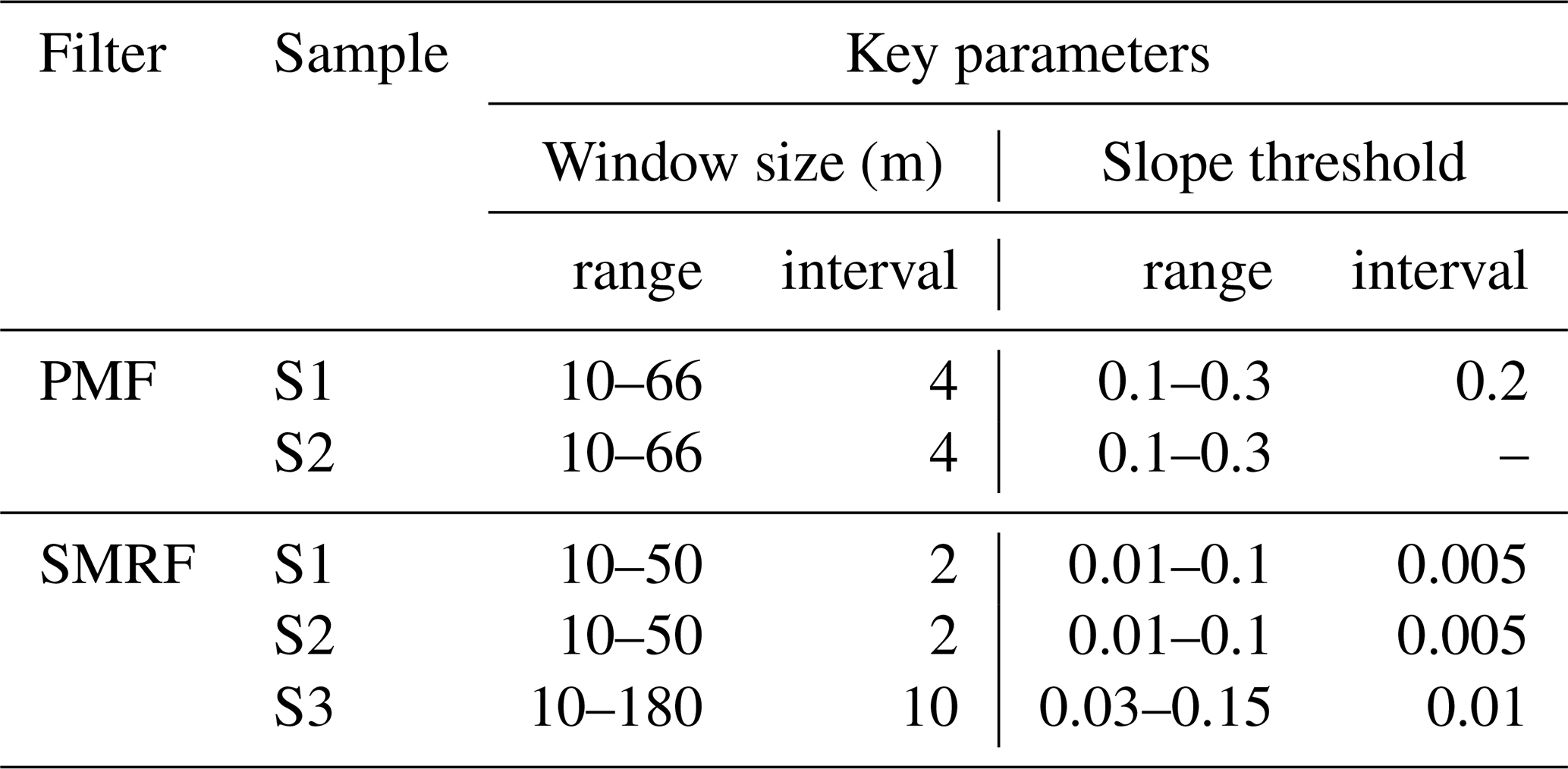
Note: the unit of the slope threshold values shown here is radian for PMF, percent of slope $/$ 100 for SMRF.

3.3 Flood inundation evaluation of the ArcticDEM-SMRF realizations

For the 192 km² area covered by sample 3 simple pluvial models were built at 10 m spatial resolution instead of the original 2 m of the ArcticDEM due to computational cost considerations. These models use DEM inputs from the lidar DTM, the original ArcticDEM, and the ArcticDEM-SMRF realizations which were filtered with various parameter combinations of the SMRF filter. The lidar DTM simulation was used as the benchmark. For modelling the pluvial inundation, the hydrodynamic model LISFLOOD-FP was used (Bates et al., 2010). The model solves the local inertial form of the shallow water equations in two dimensions across the model domain. For pluvial flood modelling, the model takes the terrain elevation and rainfall data as inputs and uses a raster-on-grid approach to calculate the velocity, water depth, and inundation (Bates et al., 2021). The input DEMs were aggregated to 10 m by averaging before being used in the flood simulation. For the ArcticDEM and ArcticDEM-SMRF models, elevation values in coastal areas (covered by water) were replaced with the lidar DTM values. This was done to remove the impact of the DEM error in non-land areas on the simulation. Rainfall data were acquired from the Climate Guide of Finland at https://www.klimatguiden.fi/articles/database-of-design-storms-in-finland (last access: 26 January 2023). It provides the database of design storms with the real momentary variations in intensity for locations across Finland. This database was generated based on radar measurements and derivations. A designed rainfall scenario with a duration of 3 h and return period of 500 years was used in the simulation. To minimize the simulation time a short duration scenario is preferred, which led to our choice of the 3 h duration. The relatively low occurring frequency (500-year return period) was then decided to avoid flood inundation being overly sensitive to the topography, which would happen when the inundation is extremely shallow. For this duration and under these return period conditions, the precipitation data at the nearest station (60.04^∘ N, 102.54^∘ E) to the city of Helsinki were used. The precipitation is 102.54 mm in total with peak intensity at 182.4 mm h⁻¹.

The simulation results were compared to the lidar DTM benchmark in terms of the simulated flood extent using the critical success index (CSI) score, the hit rate, and the false alarm ratio (FAR) defined by Eqs. (1)–(3) (Wing et al., 2017), as well as the water depth errors using the RMSE and the mean error (Eqs. 4 and 5). A wet cell is defined as one with simulated water depth exceeding 0.1 m in this paper. As is often the case in pluvial simulations, small isolated wet areas (where the number of connected wet cells was less than 15) were excluded from both the benchmark model (lidar) and the evaluation target models (ArcticDEM and ArcticDEM-SMRF) before calculating the metrics. First, all five metrics using the set of ArcticDEM-SMRF DEMs derived using different filter parameters were compared with the flooding performance of the original ArcticDEM. Then, the relationship between the five flooding metrics and the RMSE and mean error in the DEM of the ArcticDEM-SMRF realizations (aggregated at 10 m) was depicted for all land areas and urban and forest areas individually. Furthermore, the flooding performance simulated by the optimal ArcticDEM-SMRF was evaluated spatially.

$$\begin{array}{}\text{(1)}& {\displaystyle }\mathrm{CSI}={\displaystyle \frac{A}{A+B+C}}\text{(2)}& {\displaystyle }\mathrm{Hit}\mathrm{Rate}=\mathrm{100}\mathit{\%}\times {\displaystyle \frac{A}{A+C}}\text{(3)}& {\displaystyle }\mathrm{FAR}=\mathrm{100}\mathit{\%}\times {\displaystyle \frac{B}{A+B}}\end{array}$$

$$\begin{array}{}\text{(4)}& {\displaystyle }\begin{array}{rl}& {\mathrm{RMSE}}_{\mathrm{water}\mathrm{depth}}=\\ & \sqrt{{\displaystyle \frac{{\sum }_{i=\mathrm{1}}^{i=n}{\left({\text{WD}}_{i,c,\text{DEM}}-{\text{WD}}_{i,c,\text{lidar}}\right)}^{\mathrm{2}}}{n}}}\end{array}\text{(5)}& {\displaystyle }\begin{array}{rl}& {\text{Mean\hspace{0.17em} error}}_{\text{water\hspace{0.17em} depth}}=\\ & {\displaystyle \frac{{\sum }_{i=\mathrm{1}}^{i=n}\left({\text{WD}}_{i,c,\text{DEM}}-{\text{WD}}_{i,c,\text{lidar}}\right)}{n}}\end{array}\end{array}$$

A is the number of pixels which are wet in both the DEM and the lidar simulation, i.e. where the two models agree; B is the number of pixels which are wet in the DEM simulation but not the lidar simulation, i.e. overestimation; C is the number of pixels which are wet in the lidar simulation but not the DEM simulation, i.e. underestimation.

${\text{WD}}_{i,c,\text{DEM}}$ is the water depth at pixel i simulated using the DEM (ArcticDEM-SMRFs or the original ArcticDEM depending on the calculation target) within category c, and n is the number of wet cells (wet in either the lidar or the DEM simulation) within category c. Category c is defined by the land use and land cover, and they can be all land areas, urban areas, or forest areas. For example, the water depth RMSEs of ArcticDEM-SMRF in urban areas are calculated based on the ArcticDEM-SMRF pixels within urban areas.

4 Results

4.1 Optimal filter selection

The effect of using the PMF and SMRF filters to remove artefacts from the ArcticDEM in the two building-dominated samples, S1 and S2, is evaluated by plotting the error distribution and transect profiles. The filtered ArcticDEM with the smallest RMSE using each filter's optimum parameters is shown in Fig. 3. The optimal PMF parameters for S1 and S2 are window size = 42 and 30 m and slope threshold = 0.3 (radian) for both, and the optimal SMRF parameters for S1 and S2 are window size = 32 and 14 m and slope threshold = 0.08 and 0.05 (or 8 % and 5 % of slope), respectively. The calculation of error figures was conducted at 2 m pixel scale.

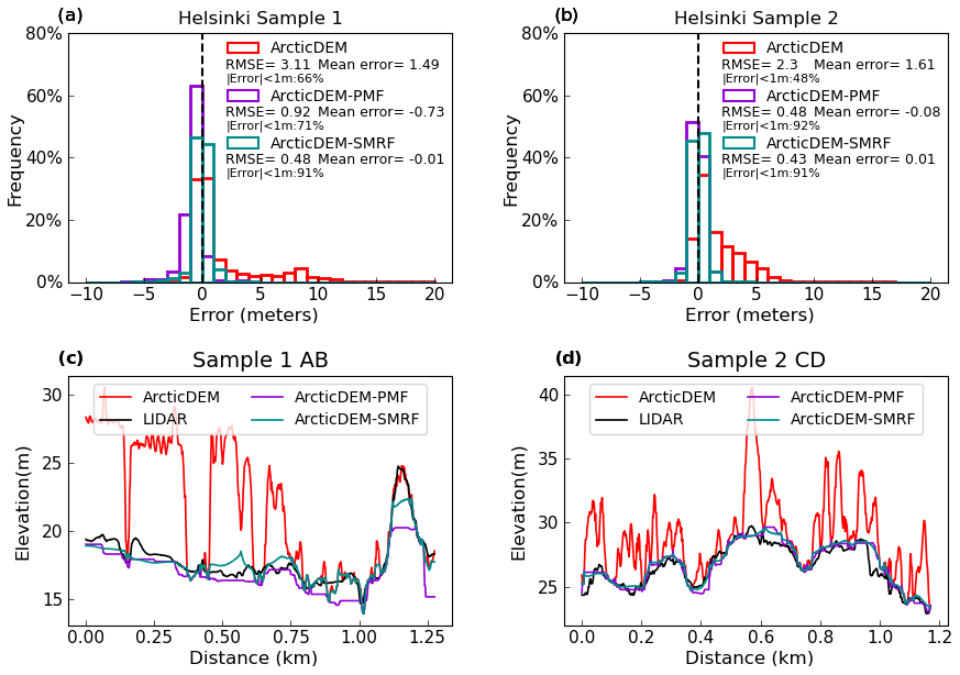
Figure 3 Error histograms of ArcticDEM, ArcticDEM with PMF applied (ArcticDEM-PMF) and ArcticDEM with SMRF applied (ArcticDEM-SMRF) for samples S1 (a) and S2 (b). Profile of ArcticDEM, ArcticDEM-PMF, ArcticDEM-SMRF, and lidar DTM for transects through S1 (c) and S2 (d). The location of transects is shown in Fig. 1b and c.

The error histograms show that both PMF and SMRF can effectively remove much of the bias caused by artefacts in ArcticDEM, with the resulting RMSE falling below 1 m in all cases. The count of pixels with error < 1 m increased to 91 % in both samples. The SMRF filter achieved a lower RMSE (0.48 and 0.43 m for S1 and S2, respectively) compared to PMF (0.92 and 0.48 m) (Fig. 3a and b). The mean error in the filtered DEMs for S1 and S2 is also evidence that SMRF has an advantage over PMF.

The DEM profile through S2 shows that SMRF and PMF work similarly well, while the profile through S1 shows that SMRF can preserve more terrain details than PMF in moderate hillslope areas (Fig. 3c; e.g. distance 0.75–1.0 km). However, both filters incorrectly identified the steepest areas of S1 as artefacts, especially PMF (Fig. 3c; distance 1.0–1.25 km). Considering both the histogram and profile results, SMRF was selected as the optimal filter to remove the artefacts from ArcticDEM for this site.

The sensitivity of the slope threshold and the window size parameter to the error metrics for ArcticDEM-SMRF at samples S1 and S2 can be found in Fig. S1 and Text S2 in the Supplement.

4.2 Bare-earth DEM generation and its error evaluation

In order to understand the effectiveness of the SMRF in a more complex urban environment the error metrics RMSE, RMSE reduction percentage, and mean error in the ArcticDEM-SMRF realizations were computed for the larger sample S3. These metrics were analysed against the window size and slope threshold parameter of the SMRF filter to evaluate the sensitivity of the ArcticDEM-SMRF error to changes in these values. As the surface artefact bias in S3 is mainly caused by buildings and forests, the analysis was conducted for all land areas, as well as for urban areas and forest areas separately (Fig. 4).

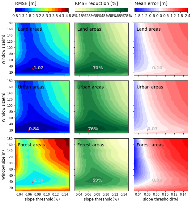
Figure 4 Surface plots of the slope threshold and the window size parameters of the SMRF filter against the RMSE, the RMSE reduction percentage, and mean error in the filtered ArcticDEM-SMRF for sample S3. The locations of the smallest values of the RMSE (which is the same as the location of the greatest values of the RMSE reduction) are marked as ×, with the values displayed. The values of the mean error at the above location are displayed and marked as +. Parameter details can be found in Table 1.

For area S3, the smallest RMSE of the ArcticDEM-SMRF realization is 1.02 m (i.e. the optimal ArcticDEM-SMRF) within all land areas, 0.84 m in urban areas, and 2.1 m in forest areas. These values represent 70 %, 76 %, and 59 % reductions in the ArcticDEM error, respectively. Although the RMSE of the optimal ArcticDEM-SMRF is greater than that computed for samples S1 and S2 (Fig. 3a and b), the magnitude of the error reduction indicates that the SMRF is still very effective at removing surface artefacts from ArcticDEM for this larger sample. The greatest reduction was achieved with a slope threshold of 0.07 combined with a window size of 30 m for all land areas or 40 m for forest areas, as well as a slope threshold of 0.06 with a window size of 20 m for urban areas. These optimum parameters are almost the same for different land covers, suggesting that the parameter choice is robust for various land-surface characteristics. For each land cover, the parameters are robust as the error removal effectiveness does not significantly drop when the parameters slightly deviate from the optimum location, and more than 40 % of the wide range of parameter combinations (234 in total) can reduce the RMSE by greater than a half. The robustness of the filter across different land covers and a range of parameters is desirable for application across large domains as this reduces the need for prior knowledge of the study site and simplifies the parameter setting.

At this site, the most effective range of slope threshold is 0.04–0.1, while the window size is from 20 to 30 m for all land areas, from 20 to 40 m for urban areas, and from 30 to 60 m for forest areas. From the parameter selection perspective within the effective range, a smaller window size is more robust and is therefore preferred because the choice of the corresponding slope threshold is broader compared with a larger window size. When the window size is smaller than 20 m, the error in the filtered DEM becomes almost independent from the slope threshold parameter choice. With some parameter combinations the SMRF becomes less effective at removing artefacts or introduces negative errors, which is a combination of large slope threshold (> 0.1) and large window size (> 60 m) or when the slope threshold is smaller than 0.04 with window size larger than 20 m. Additionally, when the window size parameter is above 60 m, the mean error in the filtered DEM becomes more sensitive to the slope threshold, especially with slope threshold smaller than 0.06.

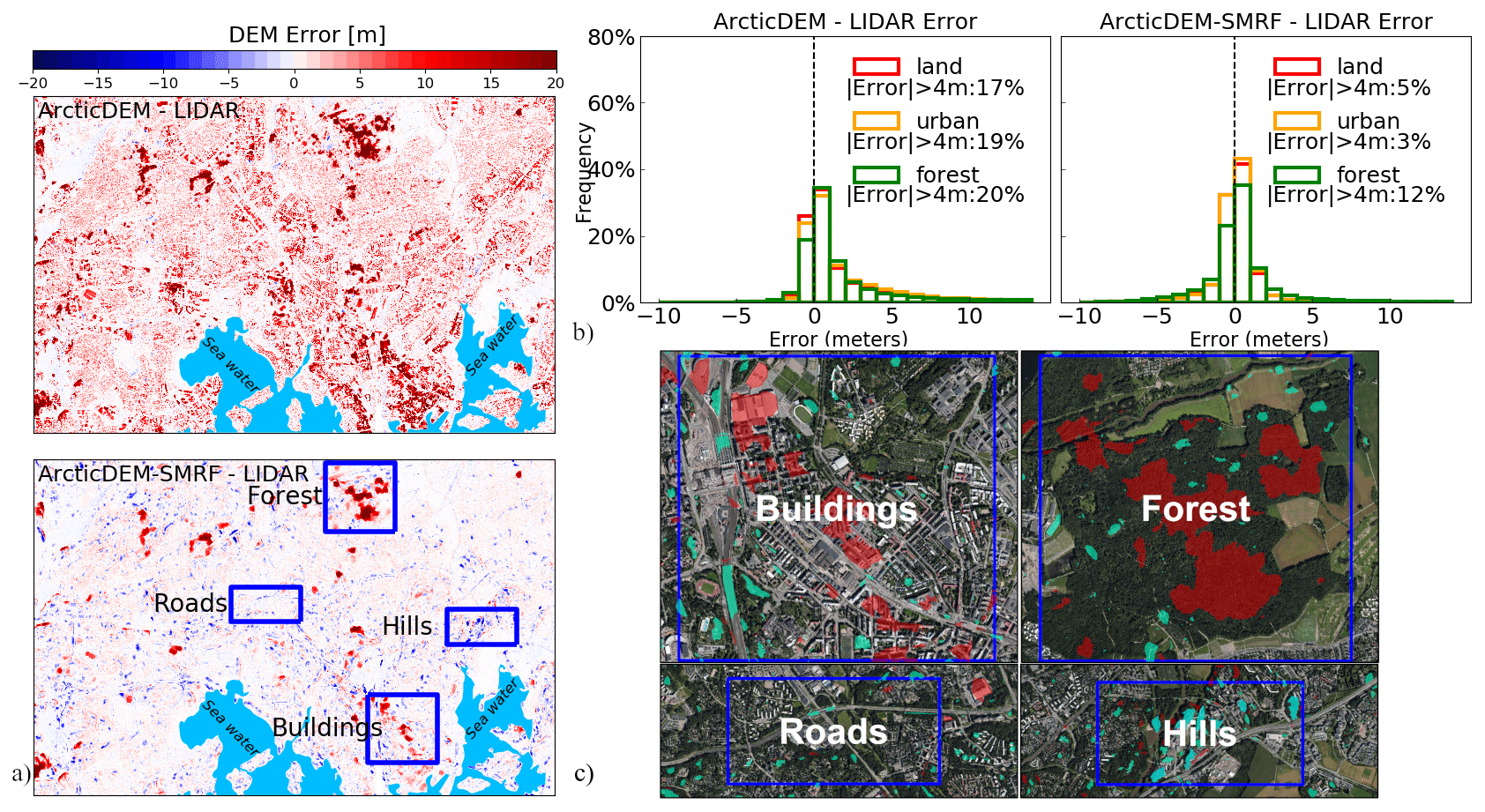
Figure 5 (a) Difference maps between the original ArcticDEM, the optimal ArcticDEM-SMRF (with slope threshold = 0.07, window size = 30 m as the SMRF parameters), and the lidar DTM at 2 m. (b) The error histograms of the original ArcticDEM and the optimal ArcticDEM-SMRF, where the calculation was conducted at 2 m pixel level. In the bottom map of (a), example locations of four features that relate to the residual errors in the ArcticDEM-SMRF are labelled. The aerial image of these locations is shown in (c), where areas with errors exceeding 4 m are marked (> +4 m as red polygons and < −4 m as green polygons, polygons are in 50 % transparency). The aerial image is an orthophotograph of Helsinki with a horizontal resolution of 8 cm, acquired during the growing season of 2017, which was accessed from Helsinki Region Infoshare at https://hri.fi/data/en_GB/dataset/helsingin-ortoilmakuvat (last access: 26 January 2023).

The error distribution of the optimal ArcticDEM-SMRF was also analysed spatially and statistically (Fig. 5). The error maps before and after applying the filter show that the SMRF method largely reduces the errors in ArcticDEM, especially in urban areas (Fig. 5a and b). Although some residual errors (> 4 m) are present in the optimal ArcticDEM-SMRF, they comprise a very small percentage (∼ 5 %) of the whole area (Fig. 5b). Errors in dense forest areas and for closely spaced buildings with large floor areas typically present as the largest positive residual errors, as shown in Fig. 5c. Large negative errors occur in hillslope areas (usually slope > 10^∘) and in some areas where above-ground traffic links such as junctions, viaducts, or overpasses are present (Fig. 5c).

4.3 Flood inundation evaluation of the ArcticDEM-SMRF realizations

The flooding evaluation metrics simulated using the original ArcticDEM and the ArcticDEM-SMRF realizations for all the 234 parameter combinations are plotted against the DEM error metrics (RMSE, mean error calculated at 10 m grid, which is the same as the flood models) for each DEM realization in Fig. 6. This analysis was conducted for all land areas and urban and forest areas separately.

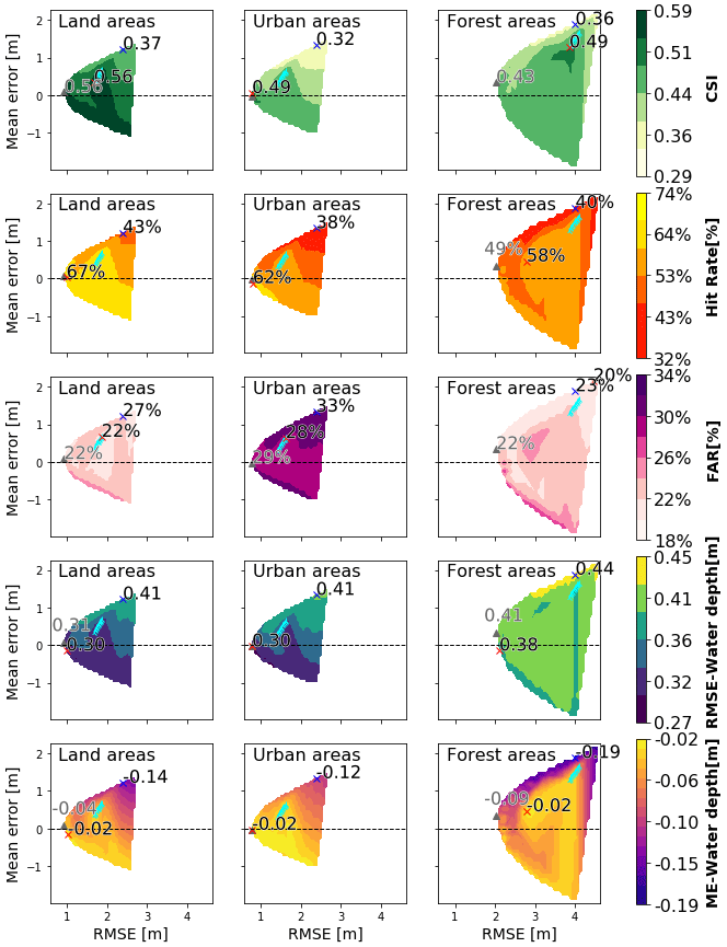
Figure 6 Surface plot of the CSI score, hit rate, FAR, the water depth RMSE, and mean error (ME) simulated using the ArcticDEM-SMRF realizations (ArcticDEM filtered using the 234 SMRF parameter combinations) at sample S3 plotted against the RMSE and the mean error in each realization member. The locations of the highest CSI and hit rate, the smallest FAR, RMSE, and the smallest absolute value of mean water depth error are marked as red crosses, with the values displayed. The location of the lowest RMSE of the ArcticDEM-SMRF are marked as triangles, with values displayed (values are not shown if both the location and value are close enough as the best flood inundation metric value). In addition, the RMSE and mean error in the original ArcticDEM are located and marked as blue crosses in each panel with the five-metric value of the original ArcticDEM simulation displayed. The locations of ArcticDEM-SMRF filtered with window size = 10 m are marked with symbols in cyan colour.

As a result of the reduced RMSE and mean error over the original ArcticDEM, the flooding performance of ArcticDEM-SMRF improved for almost all the parameter combinations. For the whole S3 area, the CSI score increased by 0.19, achieving a maximum value of 0.56 against the benchmark lidar simulation. CSI increased by 0.17 in urban areas (to 0.49) and by the slightly smaller amount of 0.13 in forest areas (to 0.49). It should be noted that although residual errors in ArcticDEM-SMRF in the defined urban areas are smaller than in other land covers, the flooding extent prediction skill does not exceed a CSI of 0.5. This is likely because the flooding extent for a pluvial simulation becomes very sensitive to the small-scale errors in the DEM in flat areas where water depths are typically quite shallow. In this sense, the simulation of pluvial flooding is a rigorous test of DEM quality, and the results achieved here using ArcticDEM-SMRF should be interpreted with this in mind. It is also important to remember that the lidar data, whilst good, are not truth and have a reported vertical error of 0.3 m. Lidar noise and systematic error also contribute to some of the difference between the flooding performance of models using the lidar and ArcticDEM-SMRF data. Simulations of fluvial flooding, where depths are typically greater, would likely score higher on the spatial extent performance metrics. The hit rate was improved by an even larger amount: 24, 24, and 18 percentage points in all land areas, urban areas, and forest areas, respectively. The FAR was reduced by 5 percentage points in all land and urban areas and 3 percentage points in forest areas. The greater improvement in urban areas provides evidence that the filter is especially effective at improving the flood simulation in urban areas, considering that flooding in urban areas is usually more fragmented and thus is more difficult to predict than in forest areas. With the ArcticDEM-SMRF, the simulated water depth error (RMSE) was reduced by up to 0.11 m (to 0.3 m) for all land areas and urban areas compared to the original ArcticDEM, and this reduction was slightly smaller (0.06 m) in forest areas. Although the water depth is still underestimated, the ArcticDEM-SMRF simulation reduced the average error by 0.12–0.17 m compared to that of the original ArcticDEM. Unlike the flooding extent performance comparison between urban and forest areas, the water depth error in urban areas is always smaller than in forest areas in both the simulation with the original ArcticDEM and the ArcticDEM-SMRF realizations. This is a result of the smaller DEM error in urban areas. Thus, it can be inferred that the water depth error is more sensitively impacted by the error in the DEM than the flood extent, at least in the case of these pluvial flooding simulations.

Unsurprisingly, the ArcticDEM-SMRF with the smallest vertical elevation error (optimum ArcticDEM-SMRF) achieved the best flooding performance scores for all land areas (marked as triangle in Fig. 6). However, there are two other cases where equally good flooding performance can be simulated using ArcticDEM-SMRF with larger error than the optimum ArcticDEM-SMRF. The first case occurs when the DEM is over-corrected by the filter, i.e. where negative errors are present in the filtered DEM (appears as strip moving from the optimal location downwards with increased RMSE and negative mean error). In this case, some steep areas are identified as objects and are flattened incorrectly. As these are not prone to be flooded, the flooding performance is barely impacted. The second case occurs when the DEM preserves the most terrain details. For all land and urban areas, these areas appear below the upper centre of surface plots and are capped by the ArcticDEM-SMRF filtered with the window size of 10 m (symbols marked in cyan colour in Fig. 6). This implies that for flood simulation the filtering strategy can perform equally well by aiming to achieve the lowest DEM error, by removing the artefacts as much as possible (over-filtering), or by preserving the terrain details (under-filtering) as much as possible.

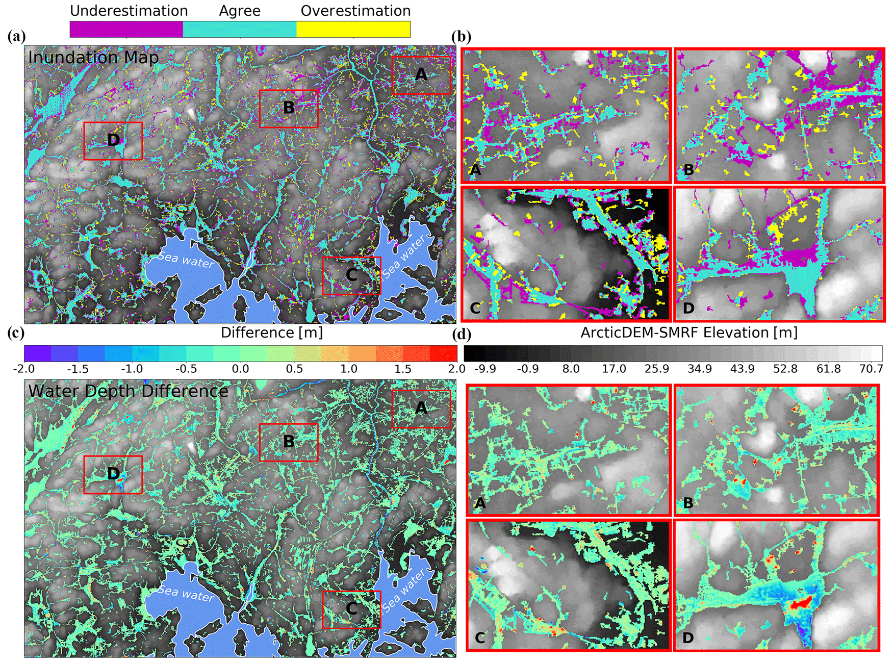
Figure 7 Inundation extent simulated using the optimal ArcticDEM-SMRF parameters (slope threshold = 0.07, window size = 30 m) at 10 m, where inundation areas that agree with, overpredict, and underpredict the extent of the lidar DTM 10 m simulation are shown in (a). The water depth difference between the ArcticDEM-SMRF and lidar DTM simulations for all wet cells is shown in (b). Areas with significant disagreement are marked by rectangles denoted A, B, C, and D with the zoomed-in maps displayed in (b) and (d). The land cover of A and C is building-dominated and of B and D forest-dominated.

The spatial distribution of the flooding extent and water depth error simulated using the optimal ArcticDEM-SMRF is shown in Fig. 7.

For a 10 m spatial resolution simulation, ArcticDEM-SMRF can capture the major flooded areas correctly with underestimation mainly around the edge of the agreed wet cells and with overestimation presenting as small, scattered patches. Total underestimated area was about 1.8 times greater than that of overestimated areas. Underestimation disproportionately occurred along traffic links and along the edge of streams, in lake areas, and in some of the forest areas with significant residual errors (Fig. 7a).

Unlike the general underestimation for the domain as a whole, both underestimation and overestimation were present in urban areas, and the number of pixels that are under- and overestimated is similar. These errors appear as disconnected patches with smaller size, and their spatial distribution is more even compared to errors in forest areas (Fig. 7b-A and b-C in contrast to Fig. 7b-B and b-D).

The greatest water depth error is present in forest areas (Fig. 7d-B and b-D) where the ArcticDEM-SMRF simulation either fails to inundate these areas (underestimation) or generates much shallower water depths compared to that simulated using the lidar DTM. In urban areas, the water depth error simulated using the ArcticDEM-SMRF is relatively small, varying between −0.5 and 0.5 m (Fig. 7d-A and d-C).

5 Discussion

5.1 The selection of ArcticDEM strips

The error in different ArcticDEM strips covering the same areas could vary significantly. In this study site, we found that the main difference in error occurs in forest areas. Within a selected 11 km² forest area the error in the strip acquired on 16 February 2015 is 12.2 m, while within the same area that of the strip acquired on 14 March 2013 was much smaller (6.66 m). From air photos, no noticeable forest coverage change was found within the selected areas between the acquisition years of the two strips. Therefore, the difference between strips could be caused by the leaf-on/leaf-off differences or the snow situation. In this case, since both acquisition dates are during the leaf-off season, it is likely a result of differences in snow cover. Even for the building-dominated samples, the error at S1 and S2 of the former strip (acquired on 16 February 2015) is 0.31 m, as well as 0.88 m larger than the latter strip. Thus, we suggest that for general bare-earth generation from ArcticDEM, different strips should consider the forest characteristics (evergreen or deciduous) and the weather conditions (snow-free or not) on the data acquisition date in overlapping areas. Strip data in leaf-off and snow-free conditions will represent more of the ground elevation compared to data collected in leaf-on or snow-covered conditions. Also, snow-free condition avoids the feature matching difficulty between stereo images in the DEM generation process, which happens often because the presence of snow results in low-contrast and repetitive image textures (Noh and Howat, 2015). The snow condition on the strip data acquisition date can be checked using the daily MODIS snow index product (Hall and Riggs, 2016).

5.2 SMRF filter parameters and transferability

A direct application of the SMRF filter proved to be effective at removing most of the surface artefacts at this study site, especially for buildings. It means that this lidar processing tool can be employed without modification in generating a bare-earth ArcticDEM in urban areas. The SMRF is robust regarding its window size and slope threshold parameter choices with respect to the error reduction in the filtered ArcticDEM. The robustness of the window size and slope threshold parameter in terms of error reduction was also demonstrated by Pingel et al. (2013), who originally proposed the SMRF filter. In theory, to remove all objects in the target areas the window size should correspond to the size of the largest object. However, this is only true for a hypothesized entirely flat area. Because in a real topography over a large domain there are always hilly areas or terrain variations, applying such a window size will identify some hilly areas as objects incorrectly and flatten them, resulting in negative errors in these areas. Therefore, a smaller window size has to be chosen instead. This smaller window size will inevitably miss out some of the larger objects. Similarly, the choice of the slope threshold has to consider preserving hilly areas (using a large slope threshold) and removing artefacts (using a small slope threshold). This inherent feature of SMRF means the choice of the window size and slope threshold needs to be balanced, which also means adjusting the window size and slope threshold to different ends in order to achieve good results. The key to applying the filter is deciding the most effective range of the parameters. In this paper, we found a range of 0.04–0.1 of the slope thresholds has overall good performance of filtering the ArcticDEM, with 0.07 generating the bare-earth ArcticDEM with the lowest error. The optimal slope threshold of 0.07 (or 7 %) is roughly the mean slope in our study site (0.077 or 7.7 %). The 30 m optimal window size corresponds to an average building density of 0.22 floor area ratio (within a 250 m grid cell) in the city of Helsinki (https://hri.fi/data/en_GB/dataset/rakennustietoruudukko, last access: 26 January 2023; Helsingin seudun ympäristöpalvelut HSY, 2022). Because we lack spatially distributed footprint data for the artefacts, we could not further quantify this relationship. The different optimum window size between urban and forest areas shows that there is a positive relationship between the optimum window size and the size of the artefacts. We suggest a slope threshold around the mean slope of the study site and a window size of 20–60 m for general application in typical urban areas, and adjusting these values up and down within this range will likely find the optimum parameter quickly in most locations. Within the reasonable range, a smaller window size proved to be more robust in that it will be less sensitive to the choice of the slope threshold.

When benchmarking to a lidar DTM simulation, similarly good flood simulation performance for the filtered DEMs is found to be achieved by the ArcticDEM-SMRF with the smallest error or negatively biased ArcticDEM-SMRF or positively biased ArcticDEM-SMRF preserving the most terrain details. Whilst the SMRF filter tends to produce negative errors in hillslopes, these areas are not flood-prone, so the flooding inundation is not significantly affected. The error sensitivity of the ArcticDEM-SMRF realizations to the SMRF parameters at different slope areas is included in the Supplement as Fig. S2 and Text S3. Applying the SMRF filter is a trade-off between the removal of artefact errors and the loss of terrain details. When the SMRF is applied with a small window size (such as 10 m), most of the terrain details can be maintained in the ArcticDEM-SMRF, while the residual error in the DEM can be large as a result of the residual artefacts with large patch sizes. Since these preserved terrain details might be important in the inundation simulation, the flood performance could be better in some places than when more of the residual errors are removed at the cost of losing these details. However, we made a further comparison of the water surface elevation error and found that positively biased ArcticDEM-SMRF does not simulate the water surface elevation as well as the other two cases. Therefore, when choosing the parameter of the SMRF, the mean slope of the target area as the slope threshold and window size around 30 m should be tested first and combinations towards the strict end (slope threshold smaller than the mean slope) of removing artefacts should take priority (as opposed to the loose end, i.e. slope threshold large than the mean slope with large window size) for generating bare-earth ArcticDEM for flood inundation modelling purposes.

5.3 Limitations

Although the SMRF filter successfully removed most of the ArcticDEM errors caused by artefacts, there is a small percentage of artefact errors (∼ 5 %) that remain in dense built-up areas and in large vegetation patches. Pixels in these areas are not entirely flagged as objects with a window size of 30 m, and some pixels are instead wrongly designated as “ground” values in the interpolation. Even though with an enlarged window size the remaining artefact errors could be removed by the SMRF, the interpolation over large patch areas would potentially be unsuccessful due to a lack of ground elevations within these zones. Additional data or a tailored approach are required to achieve the desired result in areas with large patch sizes. For building artefacts, the OpenStreetMap building footprint data (OpenStreetMap, 2023) could be helpful to predefine the areas of objects. The ICESat-2 terrain elevation might be useful to provide additional ground elevations in forest areas with large patch sizes (Neuenschwander et al., 2020; Tian and Shan, 2021).

With this filter, artefacts with a small size are usually identified before the window size reaches the maximum, and the subsequent interpolation is also more successful. This makes the SMRF filter more effective at removing building artefacts than vegetation due to the generally smaller size of building patches. However, some desired features that present similar elevated characters to building artefacts (such as traffic junctions or levees) might be removed by the filter unfavourably, and negative errors are shown in these areas. It becomes very tricky to preserve these feature heights by any automatic filtering approaches without the location information of the features. With a more sophisticated method, likely with some ancillary data, this could be possible (Wing et al., 2019). For hilly areas, some of the natural terrain might be identified as artefacts by the SMRF incorrectly, and the subsequent interpolation can cause the loss of terrain details. The error histograms of the ArcticDEM-SMRF generated with different window size parameters for four specific features (buildings and forest with large patch size, hillslopes, and roads) can be found in Fig. S3 in the Supplement. The corresponding analysis of the above is provided in Text S4 in the Supplement. Thus, in terms of the bare-earth DEM generation, the filter is likely to be less effective for areas with densely packed artefacts or hilly areas.

For flood simulation the errors in ArcticDEM-SMRF along river channels and over floodplains is particularly critical, and further DEM processing here could lead to additional improvements. In the ArcticDEM-SMRF, the elevations of the river sections that run through large patches of forest are positively biased because of the reduced effectiveness of the SMRF filter in these areas. The water depth error along the river network is expected to be mitigated once these blockages are removed, such as by using quantile regression techniques (Schwanghart and Scherler, 2017). Similarly, elevation values along the road network (acquired from OpenStreetMap) were particularly interesting and extracted for further analysis. It was found that the SMRF filter largely lowered the elevation of the road network where artefacts are present. But the resulting DEM from SMRF is interpolated based on all neighbouring pixels and not only along the road pixels on either side of the artefact removed. Thus, an unsmoothed distribution of the along-road elevation was generated, which is not ideal for flood simulation and likely to be inaccurate. A linear interpolation along the central line of the road network with a buffering around that could be used to reduce these errors in the future. It should be noted that the buffering width of the central line of roads could be tricky to define when there is not accurate road width data available.

Moreover, sinks can be present in ArcticDEM (areas with substantially lower elevation than neighbouring pixels) possibly because of the shadow effect, which is a common issue for photogrammetric DEMs (Noh and Howat, 2015). These sinks should be identified and filled in future work.

6 Conclusions

In this paper, we examine two morphological filters (PMF, SMRF) for removing surface artefacts from the ArcticDEM strip data in a complex urban environment using the city of Helsinki as a case study. We then assess the improvement in flood inundation simulation provided by the filtered ArcticDEM relative to a lidar DTM benchmark in a pluvial flooding scenario. To our knowledge, it is the first examination of the approach to generate bare-earth ArcticDEM data specifically for flood applications. It was found that the SMRF performs better at removing surface artefacts from ArcticDEM than the PMF filter, and the performance is robust with respect to its parameter setting. The most effective window size and slope threshold range are 20–40 m and 0.04–0.1 with the optimal window size achieved at 30 m and the optimal slope threshold achieved at 0.07 (or 7 %). The optimal window size positively relates to the size of artefacts, and we suggested it is set accordingly but no larger than 60 m (the upper threshold of the effective range of forest areas) for typical urban areas. The optimal slope threshold is roughly the mean slope of the city of Helsinki and is thus suggested as the first guess, and it can be adjusted up and down for optimal filter performance. With SMRF, the overall error in the ArcticDEM can be reduced by up to 70 % with the optimized parameters, achieving a final RMSE of 1.02 m.

The flood inundation simulation performance of a standard 2D hydrodynamic model was considerably improved when using the filtered ArcticDEM in that 40 % of the underestimated areas simulated by the ArcticDEM were eliminated. Although the flooding extent performance simulated by the ArcticDEM-SMRF is still not a strong match to the lidar DTM benchmark (CSI = 0.56, although some of this difference will be caused by errors in lidar itself), the pluvial flood simulation should be seen as a rigorous test as the inundated areas usually vary within a few pixels in urban areas and are easily impacted by small-scale errors. The simulated water depth error in the optimal ArcticDEM-SMRF model is comparable to the likely error in the lidar DTM simulation as a result of a ∼ 0.1 m improvement compared to the original ArcticDEM.

The residual errors in the filtered ArcticDEM are mainly composed of (1) positive errors for artefacts with large patches sizes, which are not entirely removed by the filter, and (2) negative errors in hilly areas which are incorrectly identified as artefacts. Thus, when using the SMRF filter in other study areas where the artefacts have a much higher density or artefacts with a large patch size comprising a significant proportion of the study area, the effectiveness of the SMRF filter could be less significant compared to the results of this study. Some modification of the SMRF filter might be able to remove the densely distributed artefacts, and auxiliary data are likely to be needed to guarantee satisfying interpolation results. Applying the SMRF filter to hilly areas is also likely to yield a less effective performance. From the perspective of flood inundation simulations, the SMRF parameters could be configured towards optimizing their range to generate the DEM with the lowest error or DEM with negative errors (over-filtered).

This paper suggests that applying the SMRF without any algorithm modification is effective to generate bare-earth DEMs from ArcticDEM which are likely to be applicable to other high-resolution photogrammetric DEMs and other application areas. The generated bare-earth DEM shows a largely reduced error compared to the original ArcticDEM and comparable simulated water depth error to the lidar benchmark. Thus, it is a promising alternative to lidar data for locations where such data either are not available or would not be cost efficient. In the future, using ancillary data to address the residual errors in the filtered DEM should be integrated to the bare-earth ArcticDEM generation process. To facilitate the use of bare-earth ArcticDEM in flood simulation, the blockage of residual error within rivers and errors along road networks should be carefully treated.