Assessing the ability of a new seamless short-range ensemble rainfall product to anticipate flash floods in the French Mediterranean area

Flash floods have dramatic economic and social consequences, and efficient adaptation policies are required to reduce their impacts, especially in the context of global change. Developing more efficient flash flood forecasting systems can largely contribute to these adaptation requirements. The aim of this study was to assess the ability of a new seamless short-range ensemble quantitative precipitation forecast (QPF) product, called PIAF-EPS (Prévision Immédiate Agrégée Fusionnée ensemble prediction system) and recently developed by Météo-France, to predict flash floods when used as input to an operational hydrological forecasting chain. For this purpose, eight flash flood events that occurred in the French Mediterranean region between 2019 and 2021 were reanalysed, using a hydrological-modelling chain similar to the one implemented in the French Vigicrues Flash operational flash flood monitoring system. The hydrological forecasts obtained from PIAF-EPS were compared to the forecasts obtained with different deterministic QPFs from which PIAF-EPS is directly derived. The verification method applied in this work uses scores calculated on contingency tables and combines the forecasts issued on each 1 km² pixel of the territory. This offers a detailed view of the forecast performances, covering the whole river network and including the small ungauged rivers. The results confirm the added value of the ensemble PIAF-EPS approach for flash flood forecasting, in comparison to the different deterministic scenarios considered.

1 Introduction

The year 2022, particularly the summer season, was marked by several deadly and catastrophic flash floods in Pakistan, Kentucky (USA), Iran, Sierra Leone, Bangladesh, Australia, and unfortunately many other countries. Very few parts of the world seem to be spared from flash floods. According to the World Meteorological Organization (WMO, 2020), floods are the deadliest natural hazards, and flash floods account for 85 % of the flooding events and have the highest mortality rate within the category (5000 victims annually). In France, the Mediterranean region is particularly prone to severe flash floods. Even though an intensification of extreme rainfall events in response to anthropogenic influence was diagnosed (Ribes et al., 2019), the consequences of climate change on flash floods remain unclear in this region, particularly because of the compensating effect of the expected decrease in soil moisture (Tramblay et al., 2019). However, the increase in the vulnerability to these episodes may lead to an increase in the global risk associated with flash floods in the future years.

In this context, developing flash flood forecasting is of crucial interest to limit the death toll and optimize the emergency response. Several operational flash flood warning systems have recently been developed worldwide, and they generally have similar features. The observed or forecasted rainfall can be directly compared to reference thresholds to estimate the flash flood likelihood. This is the case for instance in the Flash Flood Guidance system in the US (Clark et al., 2014) or the ERIC–ERICHA system in Europe (Raynaud et al., 2015; Corral et al., 2019). Rainfall data can also be used as input to highly distributed hydrological models, which may bring additional information about the intensity and temporal dynamics of the floods and may be particularly interesting for decision-making (Zanchetta and Coulibaly, 2020). The FLASH system in the USA (Gourley et al., 2017) and the Vigicrues Flash service in France (Javelle et al., 2016; Piotte et al., 2020) follow this second principle. The operational systems using hydrological models are still often based on radar quantitative precipitation estimates (QPEs), without involving quantitative precipitation forecasts (QPFs). This choice not only increases the quality of detection and limits the risks of false alarms but also highly limits the anticipation that cannot exceed the (limited) response times of the small catchments where flash floods do occur.

The development of convection-permitting numerical weather prediction (NWP) models has paved the way for the use of QPFs as input to flash flood warning systems, with the objective of extending anticipation lead times up to 24–48 h (Collier, 2007; Hapuarachchi et al., 2011; Zanchetta and Coulibaly, 2020). Convection-permitting models offer an interesting capacity to describe heavy precipitation events and offer space and time resolutions which are suited to the hydrological models used in flash flood warning systems. However, the current QPF products still show spatial and temporal uncertainties in the description of intense rainfall cells that may significantly exceed the typical scales of small river basins (Roberts and Lean, 2008; Clark et al., 2016; Armon et al., 2020). This may highly limit the capacity to issue relevant flash flood warnings, without appropriate strategies to represent or reduce uncertainties (Silvestro et al., 2011; Vincendon et al., 2011; Furnari et al., 2020). Even if ensemble approaches have been widely used as input to flash flood forecasting chains (Vié et al., 2012; Alfieri and Thielen, 2012; Davolio et al., 2013, 2015; Hally et al., 2015; Nuissier et al., 2016; Amengual et al., 2017; Furnari et al., 2020; Sayama et al., 2020; Amengual et al., 2021), uncertainties in QPFs can still hardly be reduced for lead times exceeding 6–8 h, even with enhanced assimilation schemes in NWP models (Davolio et al., 2017; Lagasio et al., 2019).

Efficient flash flood forecasting strategies can also be developed for short lead times (<6 h, i.e. the nowcasting range), with a high update frequency (typically 5 min to 1 h between two runs of forecasts) to regularly benefit from the last available observations (Lovat et al., 2022). For such applications, the QPF products can be derived either from adapted versions of convection-permitting NWP models (Auger et al., 2015; Benjamin et al., 2016) or by extrapolating the last radar observations (Berenguer et al., 2011; Silvestro and Rebora, 2012; Imhoff et al., 2022). Simple Lagrangian radar extrapolations can easily outperform NWP models for lead times up to 2–3 h (Mandapaka et al., 2012); however they are not suited to larger lead times because they cannot reproduce the physical changes occurring in the atmosphere. For that reason, up-to-date short-range QPF approaches now combine both information sources through blending techniques to offer a seamless transition between observed and forecasted rainfall fields (Poletti et al., 2019; Lovat et al., 2022; Scheufele et al., 2014). However, despite all these efforts to create seamless short-range QPFs products, the forecast uncertainties still remain significant and need to be quantified through ensemble approaches (Bowler et al., 2006; Seed et al., 2013; Descamps et al., 2015; Osinski and Bouttier, 2018; Bouttier and Raynaud, 2018).

The objective of this paper is to assess the potential of a new seamless short-range ensemble QPF product called PIAF-EPS (“PIAF” meaning Prévision Immédiate Agrégée Fusionnée and “EPS” meaning ensemble prediction system) and recently developed by Météo-France for flash flood forecasting purposes. This ensemble aims to represent very short-range forecast uncertainties. It can be frequently updated at a very small numerical cost, in order to keep it consistent with the latest nowcasting data based on radar images. The aim is to confirm the benefits of using such an ensemble seamless product as input to flash flood nowcasting chains, compared to other short-range deterministic QPF products from which PIAF-EPS is directly derived. For this purpose, a reanalysis of eight flash flood events observed in the French Mediterranean region between 2019 and 2021 is proposed, using a similar hydrological-modelling chain as the one implemented in the French Vigicrues Flash operational flash flood monitoring system. Since the selected flash floods mainly occurred on small rivers, the proposed evaluation framework not only focuses on a couple of gauged outlets but also offers comprehensive coverage of the small rivers hit by the studied rainfall events. This is achieved by comparing the hydrological forecasts obtained using QPFs with simulated discharges (i.e. based on QPEs) at each pixel of the hydrological-model grid (1 km resolution) and following a methodology adapted from Charpentier-Noyer et al. (2023).

The paper is organized as follows: Sect. 2 describes the hydrometeorological forecasting chains compared in the study; Sect. 3 provides details about the case studies used for the evaluation as well as the chosen verification method; and, finally, Sect. 4 presents and discusses the verification results.

Figure 1 General structure of the forecasting chains.

Figure 2 Illustration of the generation of the PIAF-EPS ensembles.

2 The short-range hydrometeorological forecasting chains

2.1 General structure of the chains

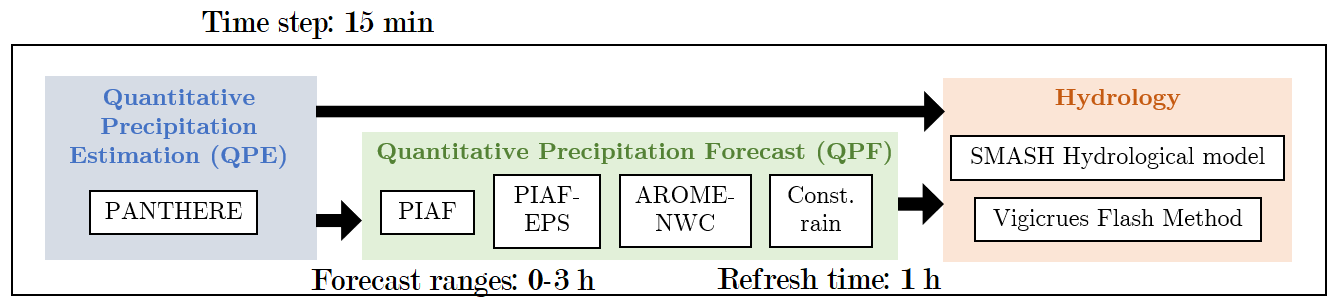
The forecasting chains applied in this study are directly inspired by the French Vigicrues Flash operational flash flood monitoring service (Javelle et al., 2016; Piotte et al., 2020). They are presented in Fig. 1. The chains evaluate the severity of the floods by comparing the simulated and forecasted hydrographs to reference discharge quantiles. These hydrological data are obtained using a fully distributed rainfall runoff model, detailed in Sect. 2.4. This hydrological model is forced with the PANTHERE (Projet Aramis Nouvelles Technologies en Hydrométéorologie Extension et Renouvellement) rainfall QPEs, derived from a network of about 30 radars over mainland France and its vicinity. (Tabary et al., 2013). As mentioned in the Introduction, the choice of using radar QPEs without QPFs would tend to limit the false alarms emitted by the chain but would also drastically limit its anticipation capacity.

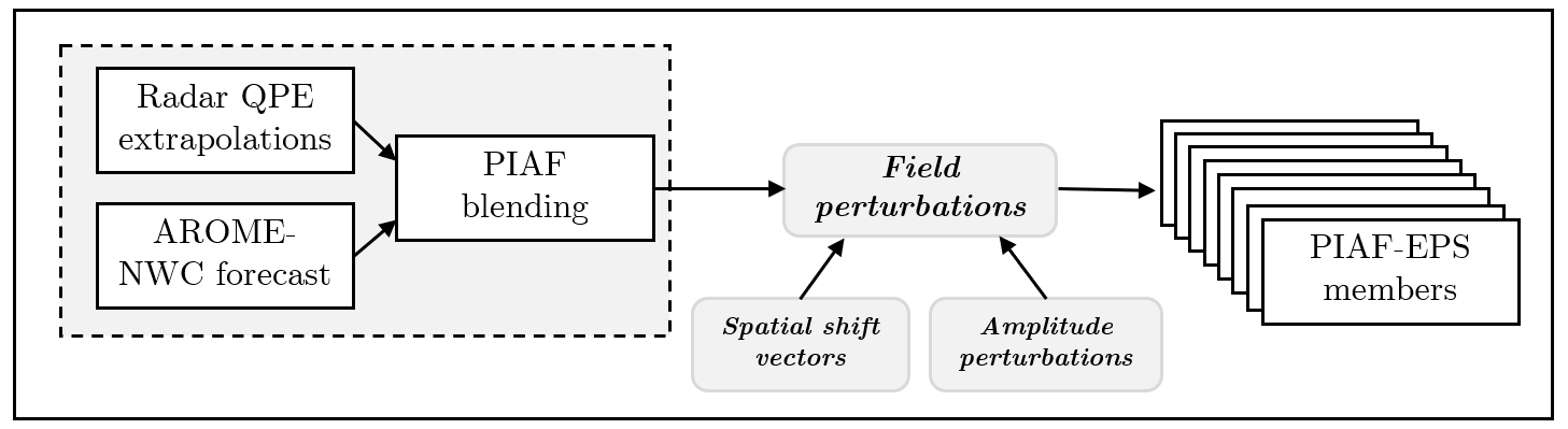
In this paper, we thus combined QPEs with different QPFs products as input of the chain, with the objective of increasing the current anticipation levels. The common time step for QPE–QPF and the hydrological model is 15 min. All the QPFs mentioned are available up to 6 h forecast lengths, but their refresh times depend on the considered product. For the present study, we decided to consider QPFs only for 0–3 h forecast ranges and with a common refresh time of 1 h. The QPF products include the new PIAF-EPS ensemble product, and three deterministic products are used as a reference. Two of these reference QPFs are directly involved in the generation of the PIAF-EPS ensemble (see Fig. 2), i.e. the deterministic version of PIAF, and the AROME-NWC numerical weather prediction model (AROME, Applications de la Recherche à l'Opérationnel à Méso-Echelle; NWC, nowcasting). The third reference QPF corresponds to a naive constant-rain scenario.

The next sections present each of the components involved in the forecasting chains applied in this study.

2.2 The three deterministic QPFs: AROME-NWC, deterministic PIAF, and naive constant-rain scenario

The first QPF product used as input to the chain corresponds to the AROME-NWC system documented in Auger et al. (2015). It is a rapid-refresh version of the AROME convection-permitting numerical weather prediction system. It is updated every hour by a 3D-Var (3D variational) data assimilation system with a 10 min observation cutoff (i.e. the initial state of each forecast is prepared using observations collected up to 10 min after its validity time), from which 6 h forecasts are produced at 1.3 km resolution with a 20 min delivery time. Each 3D-Var analysis updates the model state by multivariately blending tens of thousands of observations from various meteorological networks (radar winds and reflectivities, satellite radiances, GPS data, in situ surface and aircraft reports, etc.). More information about the AROME-NWC 3D-Var can be found in Auger et al. (2015).

The second QPF product involved is the deterministic rain nowcasting system called PIAF (Prévision Immédiate Agrégée Fusionnée in French) (Moisselin et al., 2019). Each PIAF forecast blends rainfall fields of radar QPF products and AROME-NWC numerical predictions as explained hereafter. The radar QPF product is derived from the PANTHERE radar QPEs. Rainfall accumulations are estimated every 5 min at 1 km resolution and extrapolated in time using an optical-flow technique that maintains the apparent motion of reflectivity from recent radar images. The blending of radar extrapolations and AROME-NWC follows the equation $\mathrm{PIAF}=\mathit{\alpha }\times \mathrm{radar}\mathrm{QPF}+(\mathrm{1}-\mathit{\alpha })\times \mathrm{Arome}\text{-}\mathrm{NWC}$, where α is a forecast range-dependent weighting factor. At short forecast ranges, α is equal to 1 so that PIAF is equivalent to the extrapolated radar QPF, which tends to be better than AROME-NWC. At longer forecast ranges, typically beyond 1 to 2 h, α smoothly decreases towards 0 so that the PIAF converges to the latest available AROME-NWC precipitation forecast, which consistently outperforms radar QPF at longer forecast ranges. The speed at which α decreases is case-dependent: it is determined by a simple online machine learning procedure (Auer et al., 2002; Devaine et al., 2013) that minimizes the average forecasting errors over the past 6 h, as measured by a Gerrity score over large subdomains. In a nutshell, this algorithm produces a smooth transition (as a function of forecast range) between the latest available radar extrapolation and AROME-NWC forecast; compared to climatologically optimal weights, this transition occurs earlier if AROME-NWC performed better than average during the 6 preceding hours (relative to radar extrapolation). Evaluations of the deterministic PIAF precipitation forecasts (Moisselin et al., 2019; Lovat et al., 2022) indicate that they statistically outperform both radar QPF products and AROME-NWC forecasts for forecast ranges between 0 and 3 h.

Finally, we considered a third “naive” QPF scenario, corresponding to a constant future rain. Despite its very simplistic principle, this scenario may give valuable information since flash floods are often caused by quasi-stationary storm systems (Gaume et al., 2009).

2.3 The new PIAF-EPS ensemble QPF product

PIAF-EPS is a new experimental short-range ensemble rainfall product, which is built by adding perturbations to the deterministic PIAF nowcast. The ensemble generation is original and inspired by previously proposed stochastic nowcasting schemes, e.g. those of Bowler et al. (2006) and Seed et al. (2013). The perturbation tuning parameters have been kept to a minimum, in order to facilitate future operational deployment and maintenance of the proposed system. The perturbation technique is an adaptation to nowcasting ranges of the “pertDpepi” method used by Peredo et al. (2021) and Charpentier-Noyer et al. (2023). It is illustrated in Fig. 2. Each PIAF forecast (available every 5 min) is used to generate 16 perturbed members using equiprobable perturbations of the precipitation field: spatial perturbations and amplitude perturbations.

The 16 spatial perturbations are pseudorandom shifts that approximate (together with the unperturbed forecast) a 17-member, isotropic Gaussian sample in the 2D space. The shifting vectors are computed following the recommendations and dataset of Wang et al. (2019), which include a Dirac mixture algorithm involving the Cramér–von Mises method. It is a deterministic 2D distribution that is on average a better approximation of a Gaussian than a Monte Carlo sample, given the small ensemble size. The vector directions are constant in time for each ensemble member. The vector amplitudes are scaled as a function of lead time so that the amplitude of the spatial shifts grows linearly from 0 to 30 km over 3 h, after which it is kept constant. This setting was based on a visual examination of spatial prediction errors for a set of high-impact precipitation events (independent of the ones used for the evaluations in this study).

The 16 amplitude perturbations are multiplications of 2D patterns by the spatially shifted fields. Each pattern is an independent realization of a 2D random field that has Gaussian autocorrelations in space and a serial time autocorrelation from a clipped AR(1) autoregressive process. The autocorrelation scales are set to approximately 40 km and 6 h, respectively. Thus, the amplitude perturbations are independent between members, and they slowly evolve in time. The standard deviation of the perturbation amplitude grows linearly in time for the first forecast hour, after which it is kept constant; it has been tuned to produce reliable average standard deviations of the precipitation spread (as measured by the spread–skill ratio of the whole ensemble) over a large forecast tuning sample (1 month, independent of the cases evaluated in this study). Likewise, a small bias correction (amplification of the highest precipitation intensities) of the forecasts with respect to precipitation observations has been applied using the same tuning sample. An example of the perturbations is given in Fig. 3.

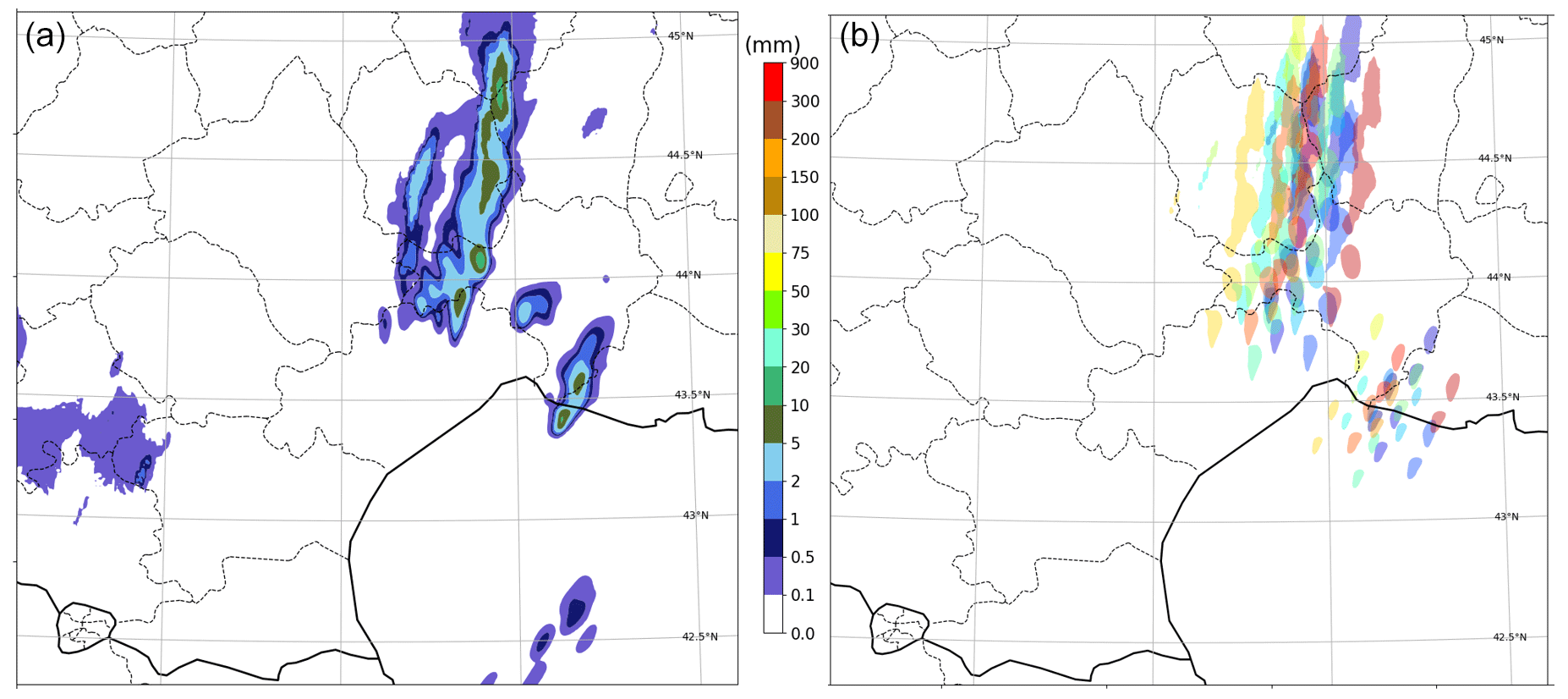
Figure 3 Example of PIAF-EPS ensemble forecast perturbations. (a) Deterministic PIAF forecast of 15 min rainfall accumulation (forecast start: 19 September 2020 at 06:00 UTC, forecast range: 2 h). This is used as member 0 of the ensemble. (b) Same field in members 1 to 16; the shading represents rainfall areas above 5 mm, with one colour for each member.

The unperturbed PIAF forecast is used as a 17th ensemble member, which makes the ensemble slightly non-equiprobable but minimizes the risk of corrupting a good deterministic forecast by applying ensemble perturbations that are too large. The justification is that, in a few high-impact cases, experience shows that intense Mediterranean precipitation can be predicted quite precisely by numerical models thanks to the influence of local orographic features. Further improvement to our (purely statistical) ensemble generation technique would be needed to automatically reduce the perturbation amplitudes in such cases, which is left for a future study.

2.4 The SMASH hydrological model and the Vigicrues Flash method

The rainfall-runoff part of the forecasting chains is based on SMASH (Spatially distributed Modelling and ASsimilation for Hydrology models). SMASH is a highly distributed, continuous, and conceptual hydrological model developed at INRAE (Institut national de la recherche pour l'agriculture, l'alimentation et l'environnement) and Hydris Hydrologie (Jay-Allemand et al., 2020). The general principle of the model is presented in Fig. 4. SMASH is inspired by the GR (Génie Rural) reservoir-based family of models (Perrin et al., 2003). For each pixel of the territory, the model includes a production reservoir (capacity c_p); a transfer reservoir (capacity c_tr); and an adapted cell-to-cell routing model, represented by a routing reservoir (capacity c_r).

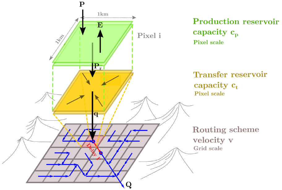
Figure 4 General outlines of SMASH (Jay-Allemand, 2020). P represents the local rainfall over one cell; E is the potential evapotranspiration; P_r is the effective rainfall; q is the elementary discharge; and Q is the total routed discharge.

The version of SMASH used in this study is the one that is currently operational in the Vigicrues Flash system. This version is working on a 1 km grid, at a 15 min time resolution. It is a “lag-0” version, which means that there is no cell-to-cell routing scheme (or, in other words, that the routing velocity is infinite): the discharge on a cell is the sum of the instantaneous discharges of all the upstream cells. This method does not provide realistic hydrographs, but this is not considered a problem, since the warning thresholds are defined based on a “climatological” run of the same model (see the next paragraph).

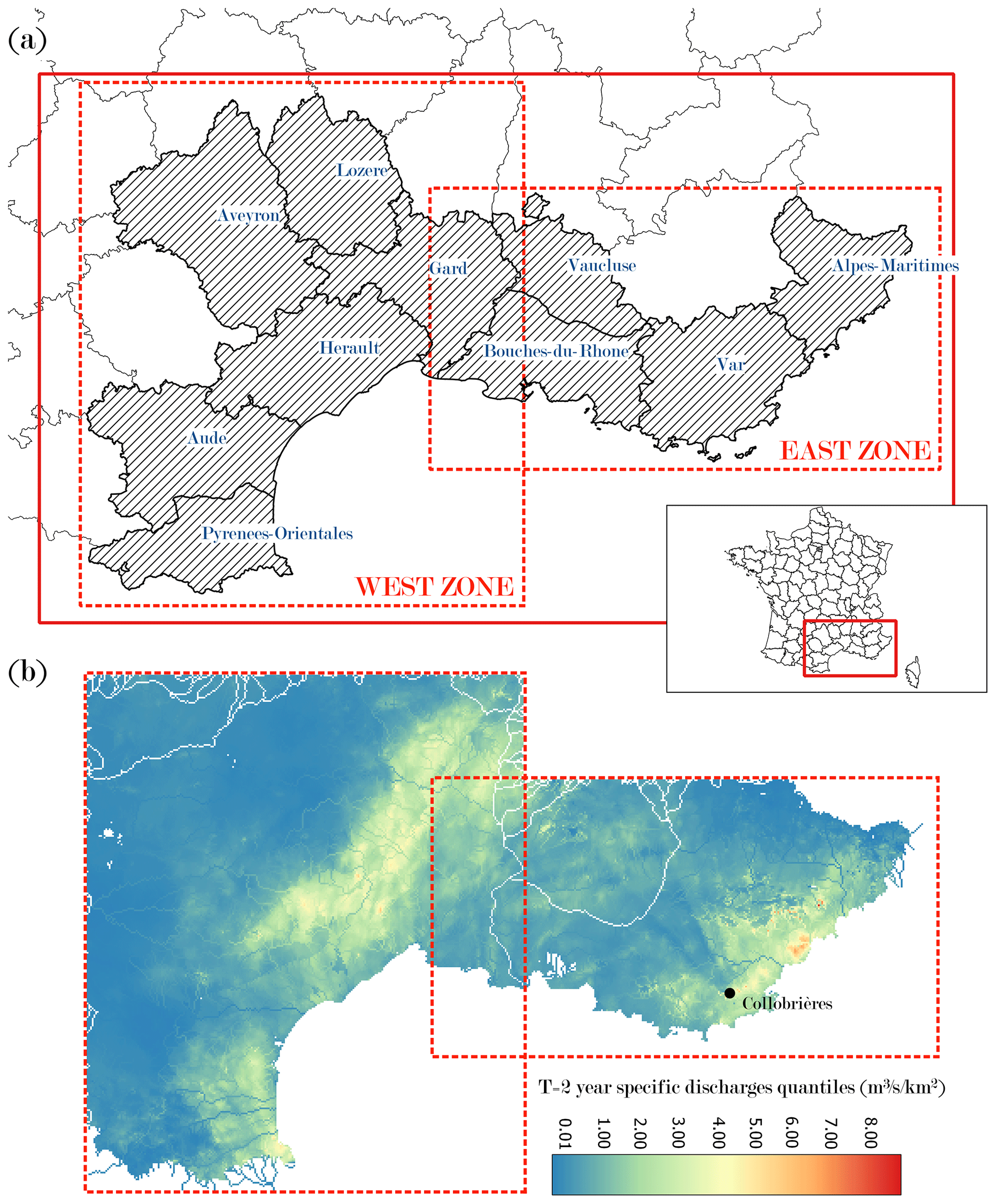
Figure 5 (a) Study area and French departments affected by the events, (b) specific discharge quantiles of T=2-year return period estimated for the study area based on a 15-year SMASH simulation.

According to the Vigicrues Flash method, the forecasted hydrographs obtained with SMASH are compared with reference discharge quantiles corresponding to defined return periods. These reference values are obtained by running the SMASH model for a long and continuous period and by adjusting a Gumbel distribution to the corresponding annual maximum series. For this study, a 15-year-long simulation period was used, which is the longest period that can be simulated based on an homogeneous PANTHERE QPE product. Discharge quantiles of T=2, 5, and 10 years were obtained for each 1 km² pixel of the studied area (see Sect. 3.1). Figure 5b illustrates the discharge quantiles obtained for the return period of T=2 years. In the west zone, the effect of relief in the Cévennes mountainous area is clearly distinguishable, logically resulting in higher rainfall amounts and higher flood quantiles. However, the results appear less consistent in the east zone, firstly because several very intense events occurred in the 2006–2021 simulation time window (sensibility to sampling) and secondly because the quality of the radar rainfall is questionable in this area. Indeed, a V-shaped band can be clearly observed, which is probably the result of bad calibration of the Collobrières radar. However this does not alter the methodology and results proposed in this study, since only simulated (and not observed) discharges are used to assess the quality of the forecast results.

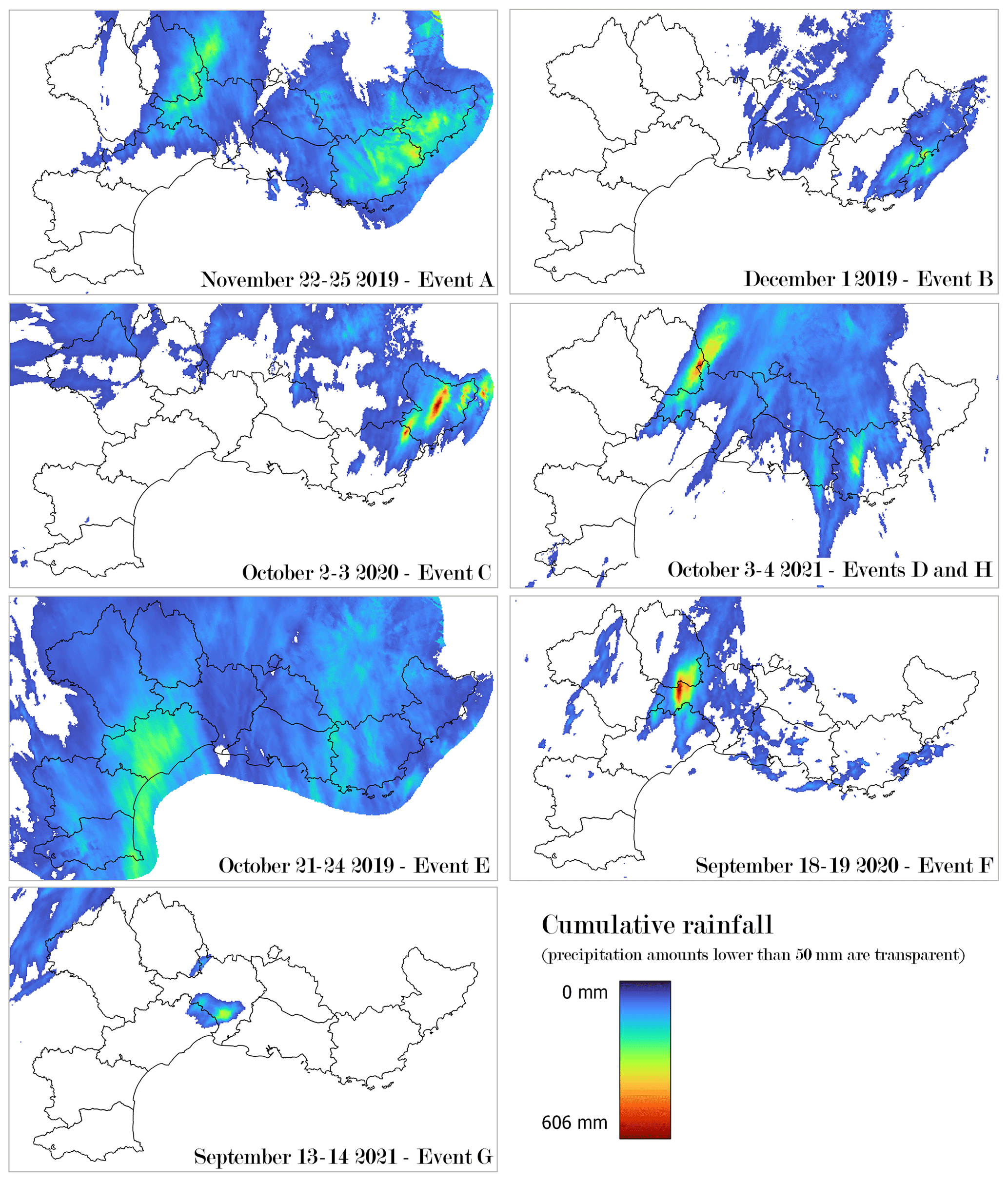
Figure 6 Maps of rainfall accumulations for each of the selected events. These maps were drawn using the ANTILOPE QPE (Champeaux et al., 2009), i.e. the best reanalysed QPE merging radar estimations and rain gauge observations.

3 Case studies and verification method

3.1 Study area and selected events

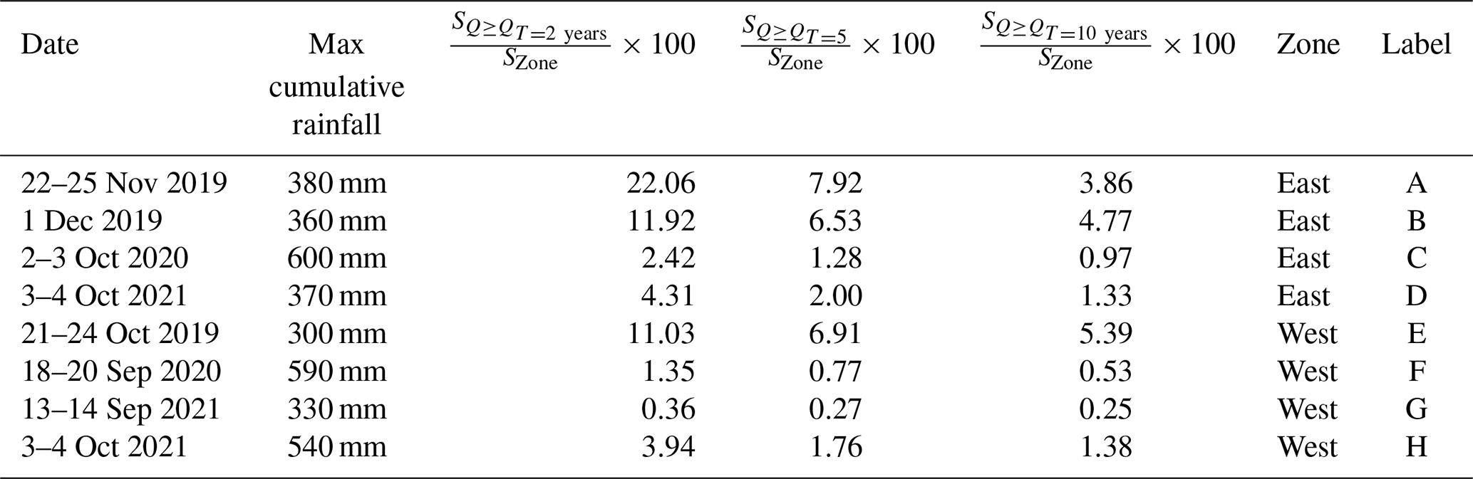
The south of France, particularly the Mediterranean region, has experienced a large number of catastrophic flash flood events this last decade, both in terms of economical damage and casualties. The study has been focused on the most recent events that hit this area, since the ensemble PIAF-EPS forecasts can be released only from February 2019 (it would be labour intensive to process older cases because of technical constraints in the archiving system, and they would be less and less relevant to current operational forecasting systems because the AROME and PIAF systems are frequently upgraded, typically once a year). Eight heavy precipitation events which occurred between 2019 and 2021 in the south-eastern region of France (see Fig. 5a) were selected. Figure 6 shows the maps of rainfall accumulations for each event, and Table 1 provides additional information including the duration, the maximum rainfall accumulation (spatial maximum), and the intensity and geographical extent of the hydrological responses simulated by the SMASH model.

Table 1 Description of the flash flood events: date; maximum rainfall accumulation (spatial maximum); percentages of the study area where the SMASH simulated peak discharge exceeds the 2-, 5-, and 10-year discharge thresholds; affected zone (by reference to Fig. 5); and assigned label.

The rainfall accumulations presented in Fig. 6 show that the selected events have very different features. Some events, such as events A and E, show a wide spread of rainfall. For these events, the larger rainfall accumulations appear homogeneous over areas covering one or several departments. The other events are much more localized and have a larger variability in rainfall accumulations. Some of them show locally very intense rainfall cells (events C, D, and F). The rainfall accumulation map for the October 2021 event shows that two separated zones were affected by the heavy rains, and the study of the QPE over time revealed that both zones were not affected at the same time: the heavy rainfall hit the department of Lozère first, on 3 October, and then the departments of Bouches-du-Rhône and Var, on 4 October. It was therefore decided to separate this event into two distinct events, labelled D and H.

For most of the eight selected events, the larger hydrological responses occurred in small ungauged catchments. However, for events A, B, and C, post-event studies could estimate the maximum peak discharge values (Lebouc and Payrastre, 2020; Brigode et al., 2021; Payrastre et al., 2022). For events A and B, it was estimated that peak discharges locally reached a 5–15 m³ s⁻¹ km⁻² range in the small basins hit by the larger rainfall accumulations. These two events are hydrologically interesting because they happened close in time and in the same area: the maximum peak discharges were probably observed during event B because of larger soil saturation and higher rainfall intensities observed on short time steps (Brigode et al., 2021). For event C (Storm Alex) which hit the same department (Alpes-Maritimes), Payrastre et al. (2022) estimated that despite significantly higher rainfall accumulations, the peak discharges were globally similar to those observed during the November–December 2019 flash flood events, except on some upstream basins where the estimated peak discharges reached values in the 15–20 m³ s⁻¹ km⁻² range. Considering these discharge values, events B and C are among the most intense floods which have been observed in the departments of Var and Alpes-Maritimes.

Because of the limited information about the actual intensity and location of the flood responses during the eight selected events, it is difficult to more thoroughly compare the characteristics of the flood events. The comparison of simulation results obtained with the SMASH model can, nevertheless, bring additional information. Table 1 gives the percentage of the surface where several discharge thresholds (2-, 5-, and 10-year return periods) were exceeded by the reference simulation. It refers to Fig. A1, which gives an idea of the extent of the flood responses exceeding these thresholds for each event. Again, we can see here that the considered flood events show very different characteristics in terms of spatial extent: from very localized events (F and G) up to more generalized flood responses (events A, B and E), according to the SMASH simulations.

3.2 Verification method

As mentioned in the Introduction, the objective is to assess the benefits of forcing the flash flood nowcasting chain with the PIAF-EPS forecasts. The whole river network of the study area, including small ungauged rivers, should be considered. As a consequence, the verification process has been applied at each 1 km² pixel of the SMASH model to provide as detailed an evaluation as possible. Since no discharge observation is generally available at this 1 km² scale, the discharge simulated by the SMASH hydrological model forced with the observed PANTHERE QPE was used as a reference. This reference also allows for ignoring the errors due to the hydrological model, the performance of which have not been assessed in this study. Therefore, in the following, Q_sim is assigned to the discharge calculated by the SMASH model forced with PANTHERE QPE, while Q_for is assigned to the discharge forecasts obtained by forcing the model with the different rainfall forecasts.

The verification process aims to evaluate if the exceedances by Q_sim of discharge thresholds Q_t are well anticipated by Q_for, i.e. when rainfall forecasts are used as input to the chain, instead of the PANTHERE QPEs. Since Q_for may correspond either to ensemble forecasts (as in the case of PIAF-EPS QPF) or to deterministic forecasts (as in the case of other QPFs), we selected verification scores that can be applied on both deterministic and probabilistic forecasts.

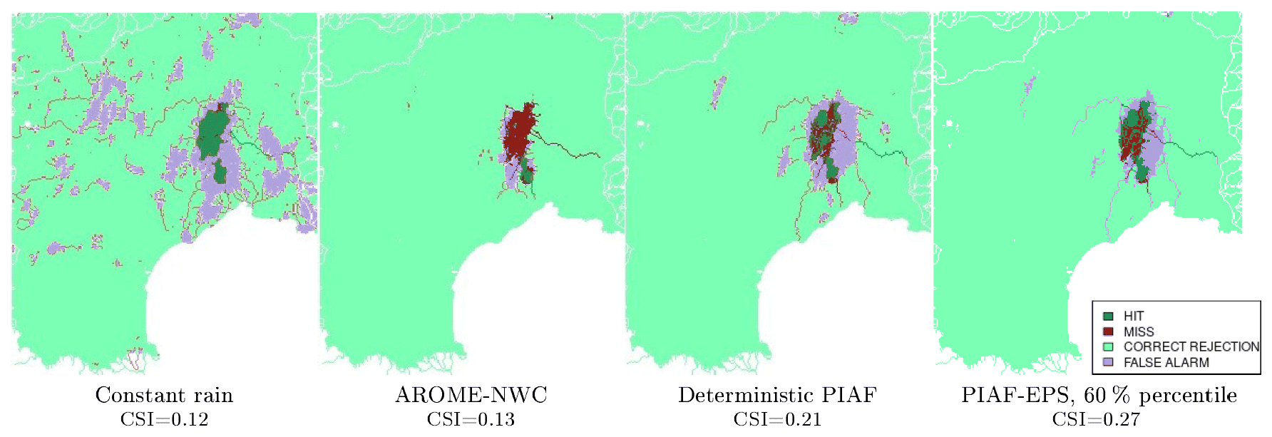
Figure 7 Maps of contingency tables for each forecast product, for the T=2-year threshold (event F).

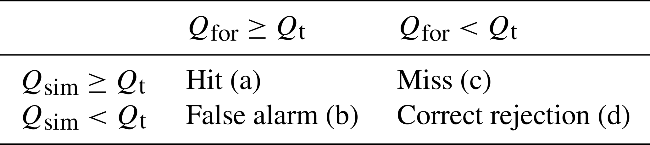
The verification is based on the filling of contingency tables, which are commonly used for assessing the ability of forecasting systems to detect binary events (Mason, 1982). The contingency tables are filled by comparing the reference (Q_sim) and forecasted (Q_for) discharges to a threshold (Q_t), resulting in the four outcomes presented in Table 2. Then, the probability of detection ($\mathrm{POD}=\frac{a}{a+c}$) and the probability of false detection ($\mathrm{POFD}=\frac{b}{b+d}$) can be calculated. In the case of ensemble forecasts, they can be plotted for different forecast probabilities for creating a ROC (receiver operating characteristic) curve (Mason, 1982).

Table 2 Content of a contingency table. Labels a, b, c, and d correspond to the number of forecasts in each category.

Contingency tables are usually filled by combining a continuous temporal sequence of forecasts, at one single site and for one unique lead time. However, we followed the principle proposed by Charpentier-Noyer et al. (2023) of building the contingency tables by aggregating the forecasts issued during the most critical phase of the event (i.e. the forecasts issued during the flood rising limb, just before the threshold exceedance by Q_sim, independently of the lead time). The detailed methodology is explained in Appendix B1. It includes a selection process of the forecasts considered to fill the contingency table, called stratification. Some adaptations have been introduced in this process in order to create a forecast-based stratification, rather than an observation-based stratification, following the recommendations of Bellier et al. (2017). The details are provided in Appendix B2.

Here we considered the forecasts obtained for each pixel of the SMASH model to build the contingency tables. Three discharge thresholds were considered at each pixel: $Q_{\mathrm{t}}=\mathit{\{}{Q}_{T=\mathrm{2}\mathrm{years}}$, Q_T=5 years, and Q_T=10 years} (see Sect. 2.4 and Appendix A). The contingency tables obtained for each threshold may be visualized directly on a map (see Fig. 7) or summarized using synthetic scores such as the POD or POFD. However, the POFD score is sensitive to the extent of the verification area, which directly determines the number of correct rejections (see Fig. 7). The choice of the verification area was already identified as an important issue by Charpentier-Noyer et al. (2023), who suggested paying particular attention to the choice of the HFA (hydrological focus area). For that reason, we chose to summary the contingency tables based on the critical success index ($\mathrm{CSI}=\frac{a}{a+b+c}$) instead of POD/POFDs. The CSI score does not take into account the correct rejections and is thus much less sensitive to the choice of the spatial verification window. This choice avoided the issue of defining an appropriate verification zone for each of the considered events.

It is important to mention that although the verification method is based on classical statistical scores, it cannot characterize the performances of the QPFs for long temporal series. We are only assessing the ability of the different QPFs to correctly predict several specific events of high intensity here. The obtained results, even if they provide interesting information, cannot be extrapolated to future events because of the limited number of events considered in this study.

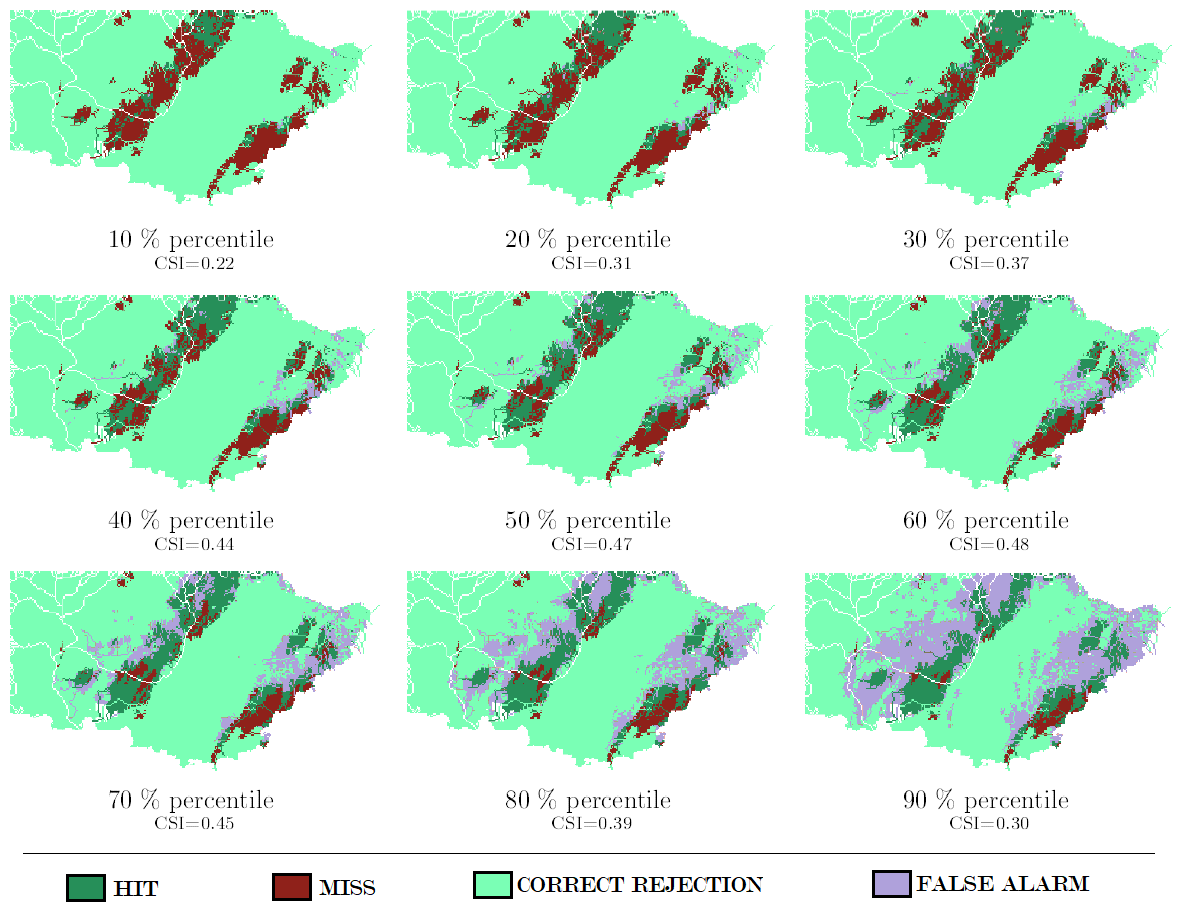
Figure 8 Map results of contingency tables for the T=5-year threshold (event B).

4 Results and discussion

4.1 Maps of contingency tables: presentation of a result sample

As explained in Sect. 3.2, the contingency tables filled for each event can be represented on maps. One map can be extracted for each discharge threshold of $Q_{\mathrm{t}}=\mathit{\{}{Q}_{T=\mathrm{2}\mathrm{years}}$, Q_T=5 years, Q_T=10 years} and each QPF product. In the case of the PIAF-EPS ensemble forecast, one map is obtained for each percentile of the forecast ensemble.

These maps allow for observing and comparing the performance of the forecasts. For example, Fig. 7 shows the maps obtained in the case of event F and a threshold of $Q_{\mathrm{t}}=Q_{T=\mathrm{2}\mathrm{years}}$. For this event, the constant rain and the AROME-NWC forecasts showed poor performance, with the first one correctly emitting warnings on the affected region but emitting many false alarms elsewhere and the other one missing most of the area affected by the event. The CSI scores summarize the content of the contingency tables (see Sect. 3.2) are 0.12 and 0.13, respectively, for these two forecasts. The improvements observed for the deterministic PIAF forecast (CSI = 0.21) confirm that, in this case, the blending of radar QPFs and AROME-NWC was effective. Moreover, the 60th percentile of the PIAF-EPS forecast, which has the highest CSI score among the other percentiles, shows even better results than the PIAF forecast (CSI = 0.27) by notably reducing the area affected by false alarms.

Figure 8 shows the maps of the contingency tables obtained for another single event (event B) and for the different PIAF-EPS percentiles. This figure illustrates the evolution of the forecast performance depending on the considered percentile of the ensemble forecast. Logically, for low percentiles, the number of correct detections is very small and much lower than the number of missed warnings, resulting in low values of CSI. For intermediate percentiles, the number of correct detections increases with respect to the number of missed warnings and false alarms, resulting in an increase in the CSI values. However, for larger percentiles, the number of false alarms increases up to the point that it outweighs the increase in correct detections, resulting in a decrease in the CSI scores.

Figure 9 CSI curves of each event for the various forecast products and thresholds.

This evolution of detection performance depending on the percentile of the ensemble forecasts directly explains the expected “hill” shape of the CSI curves presented in Fig. 9. The “best” ensemble percentiles can be identified by selecting the maximum on these curves. In the case of event B, Figs. 8 and 9 show an optimal hit–miss–false alarm balance for percentiles around 50 %–60 %.

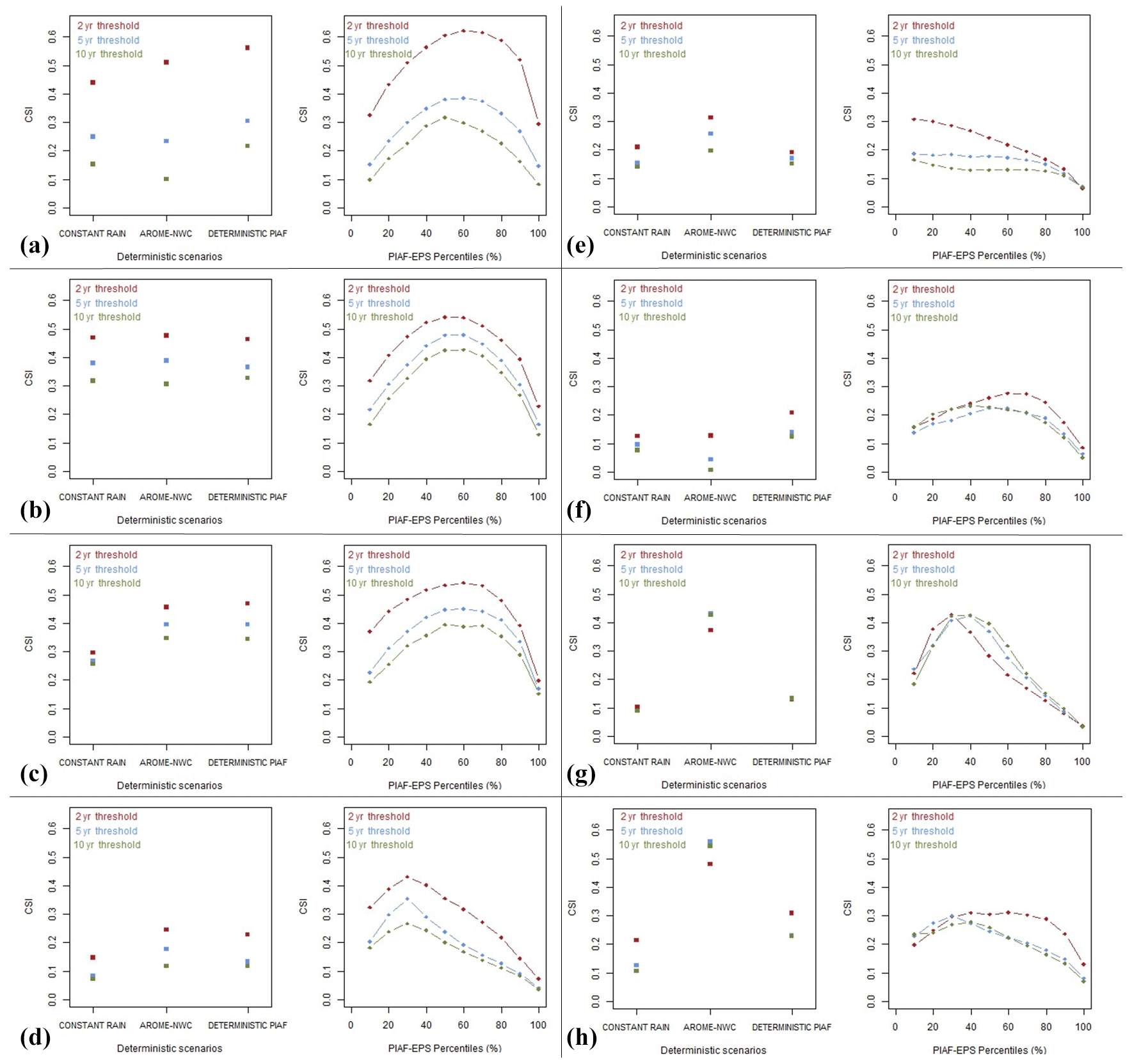
4.2 Analysis of CSI scores at the event scale

Figure 9 summarizes the CSI scores obtained for each event, each discharge threshold, and each considered forecast product. One unique CSI score is computed for the reference deterministic forecasts, whereas a CSI curve is obtained in the case of the ensemble PIAF-EPS forecast. These CSI scores provide a synthetic view, enabling the comparison of the respective performances of the different forecast approaches. For a more detailed analysis, the corresponding maps of contingency tables are presented in Fig. D1: the best-performing (i.e. maximal CSI) reference deterministic forecast is compared to the best-performing PIAF-EPS percentile, for the Q_T=10 years threshold and for each event. These maps are complementary to the CSI values presented in Fig. 9, since they allow for visualizing the geographical differences between the different QPF products, resulting in CSI differentials.

Before comparing the different forecast approaches, two generic observations can be made in Fig. 9. First, the performance of all forecasts tends to decrease as the discharge thresholds increase. This is in agreement with the theory developed by Schaefer (1990), according to which the CSI is biased by the frequency of the forecast event. Typically, the rarer an event is, the higher its return period is and the lower the CSI is. Here it leads to a CSI decrease of 0.1 to 0.2, when comparing the 2- and 10-year discharge thresholds. Second, the CSI curves for the PIAF-EPS forecasts do not always have the expected hill shape with a maximum at intermediate percentiles. In particular, for events D, E, G, and H, the maximum CSI is reached at low percentiles. It means that, for those events, PIAF-EPS had a tendency to overestimate the discharge probabilities. This is consistent with the rank diagrams plotted for each event in Appendix C (Fig. C1), which generally show a slight positive discharge bias for the same events (D, E, G, H). A larger bias can even be observed for the forecast discharges exceeding the 2-year return period threshold, even if in this specific case the bias can be increased by the stratification process (see Appendix C).

Furthermore, Fig. 9 shows that the intermediate percentiles of PIAF-EPS (i.e. 40 % to 60 %) almost systematically outperform the naive forecast approach (constant rain) and the deterministic PIAF forecast. This confirms that adding spatial and amplitude perturbations to the PIAF QPFs, in order to obtain the PIAF-EPS ensemble QPF product, resulted in better performances of the flash flood forecasts, at least for the eight intense flash floods considered in this study. The results are more mixed concerning AROME-NWC. For five out of eight events, AROME-NWC shows CSI values equivalent to or lower than the deterministic PIAF, and it is outperformed by the PIAF-EPS forecasts in these cases, at least for intermediate percentiles. Conversely, there are three events for which AROME-NWC leads to significantly higher CSI values than deterministic PIAF results (events E, G and H). For two of these three events (events E and G), PIAF-EPS largely compensates the poor performance of deterministic PIAF, leading to CSI values that are similar to AROME-NWC (events E and G). Lovat et al. (2022) have already shown that, depending on the lead time, AROME-NWC can outperform deterministic PIAF forecasts. The relationship between the CSI values and the lead times can hardly be investigated in this work, as the verification method applied looks at all the forecast runs emitted in a specific time window, regardless of their respective lead times. An explanation for the poor performance of deterministic PIAF in these events could be a sudden stationarization of the rain cells. In such a situation, the Lagrangian radar QPE extrapolation becomes a very poor rain predictor because it cannot account for rapid changes in speed in high-precipitation areas. The results obtained here suggest that PIAF-EPS can at least partly handle the inherent uncertainty in these situations, where the blending with radar QPE extrapolations limits the quality of the deterministic PIAF forecast.

4.3 Averaged CSI scores

Averaged CSI scores were also calculated in order to provide a more synthetic view of the forecast performance by aggregating them over all studied events. There are two possible ways of calculating global CSI scores:

$$\begin{array}{}\text{(1)}& {\mathrm{CSI}}_{\mathrm{1}}={\displaystyle \frac{\mathrm{1}}{N_{\mathrm{evt}}}}\sum _{n=\mathrm{1}}^{N_{\mathrm{evt}}}{\displaystyle \frac{a_n}{a_n+b_n+c_n}}\end{array}$$

and

$$\begin{array}{}\text{(2)}& {\mathrm{CSI}}_{\mathrm{2}}={\displaystyle \frac{\sum _{n=\mathrm{1}}^{N_{\mathrm{evt}}}{a}_n}{\sum _{n=\mathrm{1}}^{N_{\mathrm{evt}}}{a}_n+b_n+c_n}}.\end{array}$$

Since the studied events have very different spatial extents (see Fig. A1 and Table 1), we chose to use the CSI₁ formula, where the averaging implies that all the events have the same weight. CSI₂ would have given much more relative weight to the large-scale events.

The global CSI curves obtained from CSI₁ are presented in Fig. 10 and indicate that, globally, PIAF-EPS 30th–60th percentiles outperform all the deterministic reference forecasts. This identification of best percentiles can be useful for end users (WMO, 2012), particularly if they remain relatively stable depending on the considered events. In this paper, we assess the value of these best percentiles in a slightly overoptimistic way, since we use all events to derive the optimum CSI values (i.e. it is not an “out-of-sample” optimization) because our sample is very small. This methodological weakness does not invalidate our conclusions, however, since the CSI curves are rather stable from case to case in our sample. The global CSI₁ scores also confirm that AROME-NWC globally performs better than PIAF for the eight studied events. However, this conclusion is largely influenced by events G and H, for which the CSI differences between AROME-NWC and deterministic PIAF results are the largest.

Figure 10 Averaged CSI scores calculated for the eight flood events.

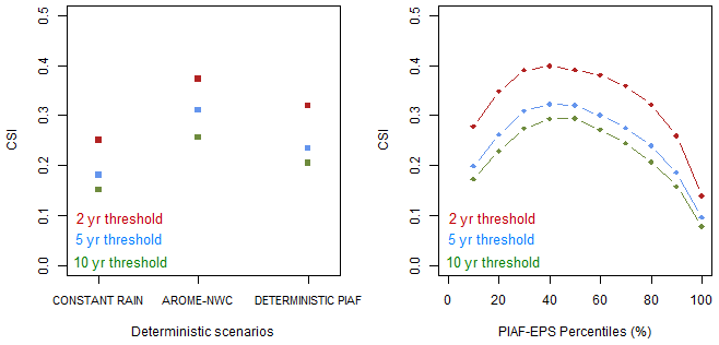
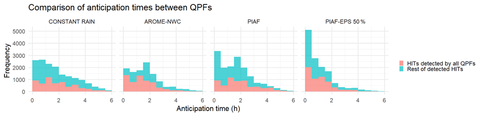
Figure 11 Anticipation times aggregated for all events and for each QPF (50th percentile for PIAF-EPS) for the 5-year threshold.

Finally, the averaged CSI values obtained with the intermediate percentiles (40 %–50 %) of PIAF-EPS are in the 0.3–0.4 range, depending on the return period of the discharge threshold considered. The CSI scores can reach up to 0.6 for some specific events. These CSI values may appear relatively low from the perspective of operational decision-making. However, the real added value of these forecasts for decision-making can only be evaluated by considering the balance between the gains associated with the hits and the costs related to false alarms. Moreover, other studies dealing with flash flood nowcasting found similar CSI values of 0.20 (Clark et al., 2014) and 0.38 (Gourley et al., 2017), even though these CSI values were obtained in very different contexts (using observations over the whole US) and thus cannot be directly compared with the values of this paper.

4.4 Anticipation lead times

The CSI scores presented above assess the ability of the rainfall products to predict discharge threshold exceedances, regardless of anticipation. However, maximizing the anticipation times of good forecasts is another desirable property in an operational forecasting context. An estimation of the anticipation times associated with the hits in contingency tables was proposed by Charpentier-Noyer et al. (2023) by computing the difference of t_sim−t_run, where t_sim represents the first threshold exceedance by the reference simulation and t_run corresponds to the starting time of the first forecast that identifies this threshold exceedance event. Anticipation times for each QPF (50th percentile for PIAF-EPS, as intermediate percentiles were identified as optimal in the previous section) and for the 5-year threshold are presented in Fig. 11. Firstly, the results show that the anticipation times can reach up to 6 h. This is due to the choice of counting a hit when t_sim falls within the interval ]t_run; $t_{\mathrm{run}}+T+\mathrm{3}$ h] (see Appendix B2), with T being the forecast range ($\mathrm{0}<T\le \mathrm{3}$ h). Anticipation times exceeding the forecast length of 3 h, even if helpful in anticipating threshold exceedances, result from unrealistic forecasts where the threshold crossing is forecasted too early. It is thus logical to observe that the constant-rain scenario has the highest number of anticipation times exceeding 3 h, and it is rather satisfying to note that PIAF-EPS has the least occurrences in this anticipation range. The comparison of histograms in the 0–3 h range of anticipation times confirms that PIAF and PIAF-EPS yield a larger number of hits globally. Additionally, it shows that this increase of hits is primarily obtained in the 0–2 h range of anticipation times compared to AROME-NWC. This logic is clear as it corresponds to the forecast range where radar extrapolations are involved in building PIAF and PIAF-EPS. Furthermore, it suggests that PIAF-EPS brings additional hits mainly in the 0–1 h range of anticipation times when compared to PIAF. However, drawing systematic conclusions is complicated, as we are only examining one ensemble percentile here, and we are considering all events, while important differences may exist within each event.

5 Conclusions

The development of efficient tools and methods for flash flood forecasting is of crucial importance to limit the often catastrophic consequences of flood hazards. The objective of verifying newly developed forecasting methods and products is a key step before their integration into operational forecasting suites. In the current study, the potential of the experimental PIAF-EPS short-range ensemble rainfall product for flash flood forecasting purposes has been assessed. Eight heavy precipitation events that occurred between 2019 and 2021 in the south-eastern region of France were reanalysed using a hydrological forecasting suite similar to the one that is currently operational in the French national flash flood warning system, Vigicrues Flash. An original verification process, directly derived from Charpentier-Noyer et al. (2023), was performed on each 1 km² pixel of the area. This allowed us to plot maps to precisely visualize the forecast performance and to summarize it as CSI scores.

The hydrological forecasts based on PIAF-EPS have been compared to those obtained with deterministic PIAF and AROME-NWC rainfall forecasts, since PIAF-EPS is directly obtained from these two deterministic products. A naive constant-rainfall scenario was also used as a reference. The results showed that PIAF-EPS systematically outperformed the constant-rainfall and the deterministic PIAF forecasts. As indicated in previous studies, it was also observed that PIAF does not always outperform AROME-NWC because the forecast quality depends on the lead time and on the performance of radar QPE extrapolations. Over the eight events considered in this study, it was observed that the PIAF-EPS performance is generally similar to, or better than, AROME-NWC.

In a nutshell, the results obtained confirm the added value of using the PIAF-EPS products for anticipating flash floods in the Mediterranean area. We argue that statistical scores such as the CSI provide valuable indications of performance despite being applied not on long data series but rather on only eight particularly intense flash floods. Indeed, when assessing the performance of such a new forecasting product, it is essential to carefully check its behaviour on some high-impact events, as a complement to more generic statistical evaluations. The results presented here should nevertheless be complemented with more robust statistical evaluations over longer periods of time and on a larger number of high precipitation events, bringing a more generic overview of the quality of the forecast ensembles.

Appendix A: Hydrological presentation of the studied events

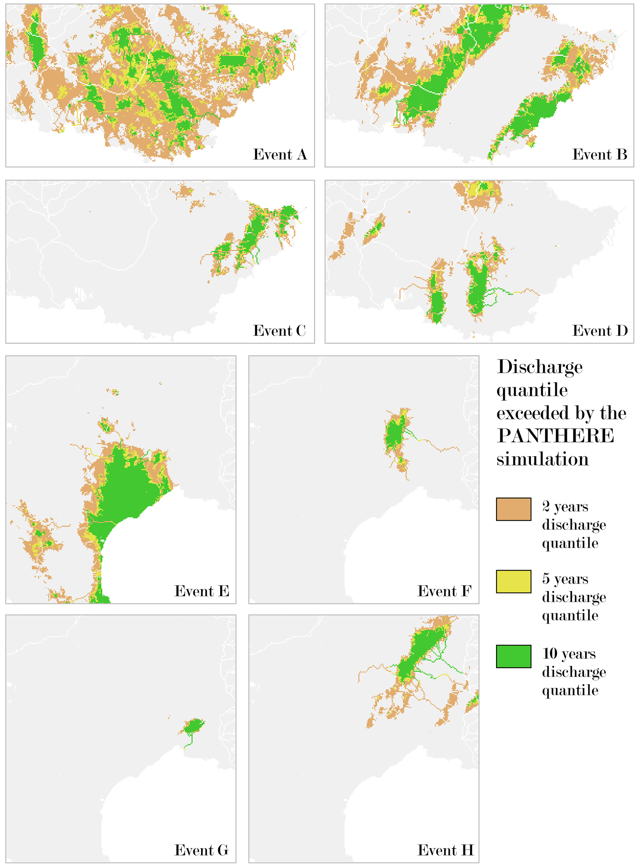
Figure A1 Discharge quantiles exceeded by the PANTHERE simulation (Q_sim) during each event.

Appendix B: Methodology for filling the contingency tables

The contingency tables are filled for each pixel of the zones. For an ensemble forecast product, each percentile is considered separately to be treated as a deterministic product. For each pixel, we look at the hydrograph of Q_sim(t) simulated by SMASH with the PANTHERE QPE as input and at the hydrographs of Q_for(t) forecasted by SMASH when forced with a QPF product (constant-rain scenario, AROME-NWC, PIAF, or PIAF-EPS percentiles). Let t_run be the forecast start time, T be the forecast range ($\mathrm{0}<T\le \mathrm{3}$ h), and Q_t be the considered discharge threshold.

B1 Detailed method of Charpentier-Noyer et al. (2023): observation-based stratification

The method, applied on each spatial entity and for each forecast probability, is as follows.

1. If there exists t such that Q_sim(t)≥Q_t, then the date t_sim corresponding to the first threshold exceedance by Q_sim is selected. A sample S consists of all the pairs (t_run, T) such that $t_{\mathrm{run}}<t_{\mathrm{sim}}\le t_{\mathrm{run}}+T$ is constructed.

   • If there exists (t_run, T)∈S such that $Q_{\mathrm{for}}(t_{\mathrm{run}},T)\ge Q_{\mathrm{t}}$, a hit is counted. The t_run corresponding to the first threshold exceedance is selected to calculate the anticipation time: t_sim−t_run.

   • If $Q_{\mathrm{for}}(t_{\mathrm{run}},T)<Q_{\mathrm{t}}\forall (t_{\mathrm{run}},T)\in S$, a miss is counted.

2. If $Q_{\mathrm{sim}}\left(t\right)<Q_{\mathrm{t}}\forall t$, the date t_sim corresponding to the global maximum of Q_sim is selected and a sample S consisting of all the pairs (t_run, T) such that $t_{\mathrm{run}}<t_{\mathrm{sim}}\le t_{\mathrm{run}}+T$ is constructed.

   • If there is $(t_{\mathrm{run}},T)\in S$ such that $Q_{\mathrm{for}}(t_{\mathrm{run}},T)\ge Q_{\mathrm{t}}$, a false alarm is counted.

   • If $Q_{\mathrm{for}}(t_{\mathrm{run}},T)<Q_{\mathrm{t}}\forall (t_{\mathrm{run}},T)\in E$, a correct rejection is counted.

B2 Adapted method: forecast-based stratification

The detailed process used to build the contingency table is as follows.

1. If there exists (t_run, T) such that $Q_{\mathrm{for}}(t_{\mathrm{run}},T)\ge Q_{\mathrm{t}}$, the pair (t_run, T) corresponding to the first threshold exceedance by Q_for is selected.

   • a.

     If $Q_{\mathrm{sim}}\left(t\right)<Q_{\mathrm{t}}\forall t$, a false alarm is counted. See Fig. B1a.

   • b.

     If there is t such that Q_sim(t)≥Q_t, the first threshold exceedance occurs at t_sim.

     • If t_sim∈]t_run, $t_{\mathrm{run}}+T+\mathrm{3}\mathrm{h}]$, a hit is counted. The anticipation time is equal to t_sim−t_run. The time interval ]t_run, $t_{\mathrm{run}}+T+\mathrm{3}\mathrm{h}]$, particularly the +3 h part, was chosen in order to create a tolerant window for the hit counting. It seemed coherent to use a time tolerance equal to the maximum lead time. See Fig. B1b.

     • If $t_{\mathrm{sim}}>t_{\mathrm{run}}+T+\mathrm{3}$ h, a false alarm is counted. See Fig. B1c.

     • If t_sim≤t_run, a miss is counted. See Fig. B1d.

2. $Q_{\mathrm{for}}(t_{\mathrm{run}},T)<Q_{\mathrm{t}}\forall (t_{\mathrm{run}},T)$ is as follows.

   • If $Q_{\mathrm{sim}}\left(t\right)<Q_{\mathrm{t}}\forall t$, a correct rejection is counted. See Fig. B1e.

   • If there exists t such that Q_sim(t)≥Q_t, the first threshold exceedance occurring at t_sim, a miss is counted. See Fig. B1f.

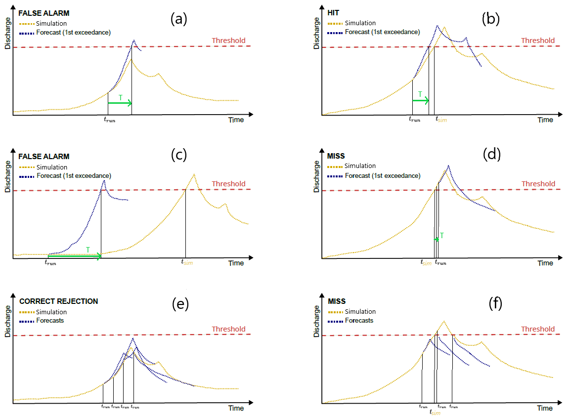
Figure B1 Six possible cases in the new methodology (inspired by Charpentier-Noyer et al., 2022): (a) forecasted threshold exceedance not present in the simulated hydrograph (false alarm), (b) threshold exceedance correctly forecasted (hit), (c) threshold exceedance anticipated but with anticipation largely exceeding the forecast lead time (false alarm), (d) threshold exceedance detected by one forecast but right after the simulation (miss), (e) absence of threshold exceedance in the simulation and in the forecasts (correct rejection), and (f) threshold exceedance undetected by all the forecasts (miss).

Appendix C: Rank diagrams

Rank diagrams, also called Talagrand diagrams (Candille and Talagrand, 2005), are one of the most common tools for assessing the reliability of meteorological ensemble forecasts. The general idea of this tool is to count the number of times the observation value is included in a given interval of the ensemble forecast quantiles. As a consequence, if the observation value is often close to low quantiles, it means that the forecast model has a tendency to overestimate. On the other hand, if the observation is more often close to high quantiles, then the model tends to underestimate. Logically, a perfect diagram would be perfectly flat, which would mean that the observation is uniformly distributed among the ensemble forecast quantiles. However this never happens in reality. The rank diagram is useful to quickly detect biases in an ensembleforecast. It can detect not only positive or negative biases but also under- and overdispersion of the ensemble forecasts. Traditionally, the rank diagram is applied to rainfall ensemble forecasts. However, in this study it was applied to discharge ensemble forecasts, at each pixel of the SMASH model computation grid. The rank diagrams presented here combine all the forecasts issued during each event and are computed for a fixed lead time (1 h).

In order to distinguish the roles of high and low discharges in the rank diagram form, it was decided to build separate rank diagrams for each category. However it is necessary to take precautions concerning the criteria that distinguish those categories. Indeed, Bellier et al. (2017) have shown that a sample stratification based on the observations can introduce bias. A sample stratification based on forecasts is recommended in most of the cases. Therefore, the following categories were chosen:

• $Q_{\mathrm{med}}\le \frac{\mathrm{1}}{\mathrm{2}}{Q}_{T=\mathrm{2}\mathrm{years}}$ for low discharges,

• $\frac{\mathrm{1}}{\mathrm{2}}{Q}_{T=\mathrm{2}\mathrm{years}}<Q_{\mathrm{med}}\le Q_{T=\mathrm{2}\mathrm{years}}$ for medium discharges,

• $Q_{\mathrm{med}}>Q_{T=\mathrm{2}\mathrm{years}}$ for high discharges,

where Q_med is the median discharge of the hydrological ensemble forecasts and Q_T=2 years is the 2-year return period quantile, according to the historical run of the SMASH model.

Note that, even if based on forecast discharges, this stratification can still cause bias: when only the areas and time steps with high forecast discharges are considered, the overall probability that the considered forecasts exceed the observed discharges tends logically to be higher and vice versa. However, this stratification effect does not affect the global rank diagrams.

Figure C1 Rank diagrams obtained for each event: 1 h lead time.

Appendix D: Maps of contingency tables for each event

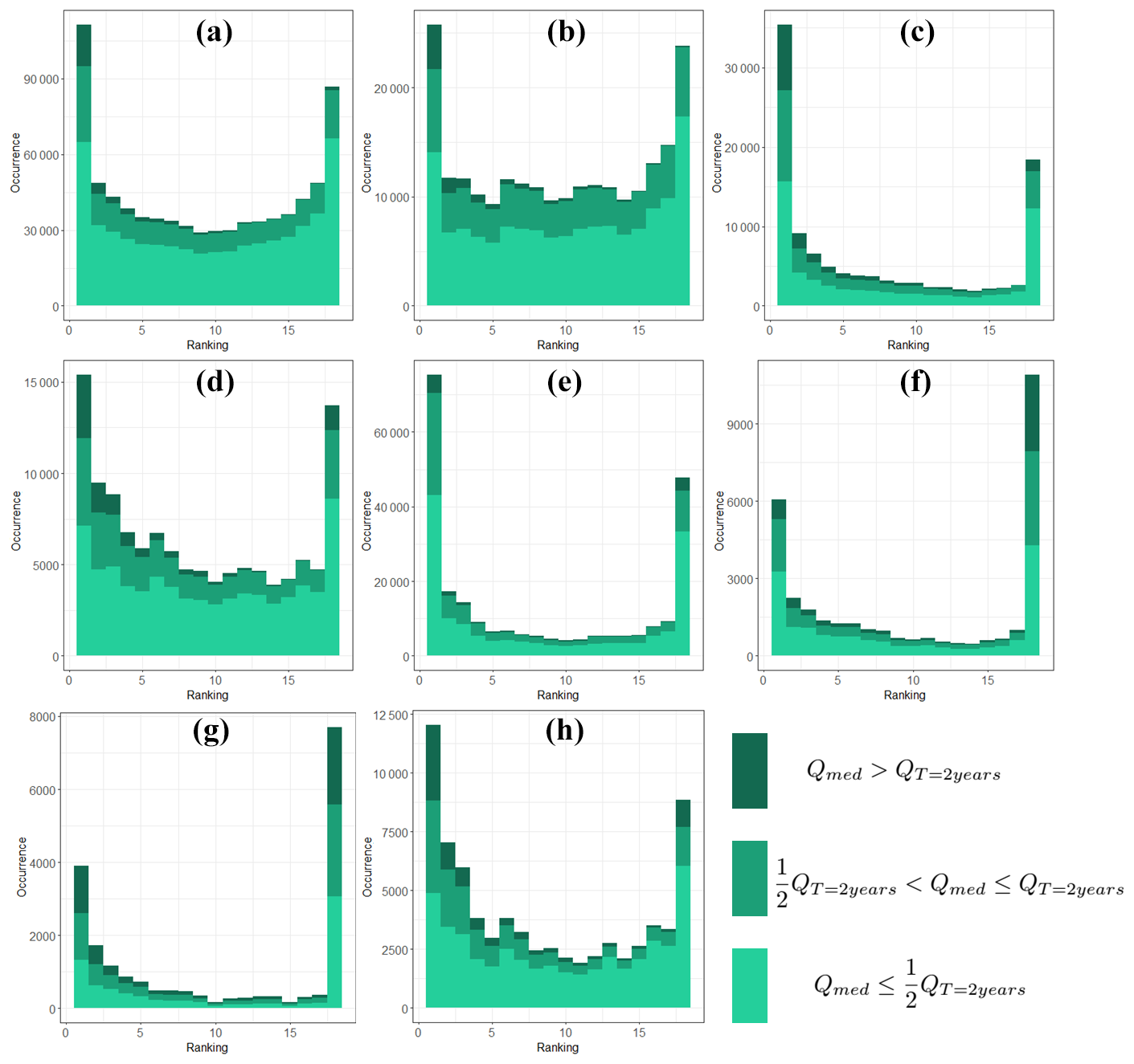
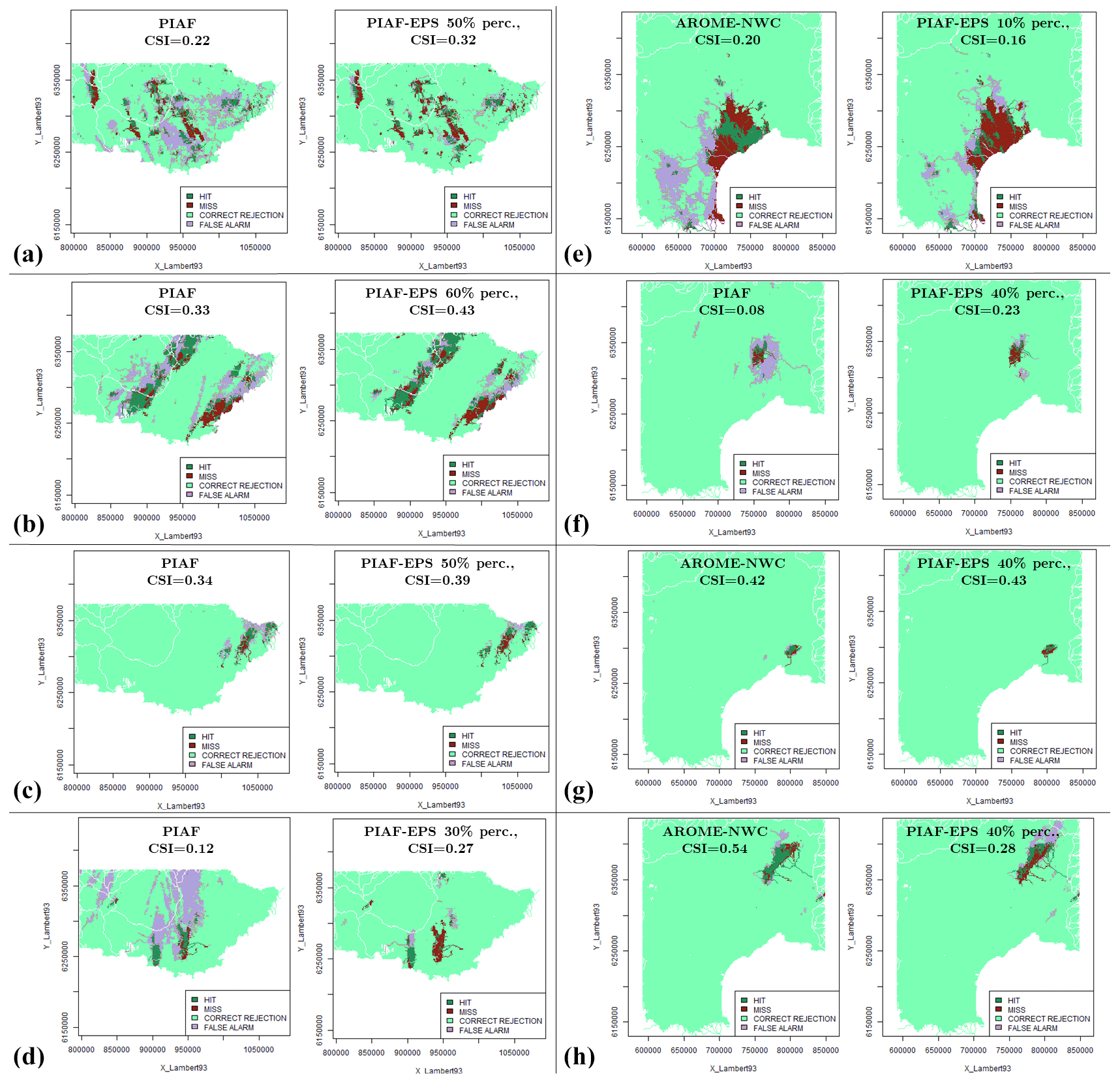
Figure D1 (a–d) Best deterministic forecast and (e–h) best PIAF-EPS percentile in terms of CSI, for the T=10-year threshold for each event.