the Creative Commons Attribution 4.0 License.
the Creative Commons Attribution 4.0 License.
 | 27 Sep 2023
Sensitivity analysis of erosion on the landward slope of an earthen flood defense located in southern France submitted to wave overtopping
Clément Houdard
Adrien Poupardin
Philippe Sergent
Abdelkrim Bennabi
Jena Jeong
The study aims to provide a complete analysis framework applied to an earthen dike located in Camargue, France. This dike is regularly submitted to erosion on the landward slope that needs to be repaired. Improving the resilience of the dike calls for a reliable model of damage frequency. The developed system is a combination of copula theory, empirical wave propagation, and overtopping equations as well as a global sensitivity analysis in order to provide the return period of erosion damage on a set dike while also providing recommendations in order for the dike to be reinforced as well as the model to be self-improved. The global sensitivity analysis requires one to calculate a high number of return periods over random observations of the tested parameters. This gives a distribution of the return periods, providing a more general approach to the behavior of the dike. The results show a return period peak around the 2-year mark, close to reported observation. With the distribution being skewed, the mean value is higher and is thus less reliable as a measure of dike safety. The results of the global sensitivity analysis show that no particular category of dike features contributes significantly more to the uncertainty of the system. The highest contributing factors are the dike height, the critical velocity, and the coefficient of seaward slope roughness. These results underline the importance of good dike characterization in order to improve the predictability of return period estimations. The obtained return periods have been confirmed by current in situ observations, but the uncertainty increases for the most severe events due to the lack of long-term data.
- Article
(1864 KB) - Full-text XML
- BibTeX
- EndNote


The site of Salin-de-Giraud located in the Camargue area in southern France is a historically low-lying region and is thus frequently exposed to numerous storms. The latest Intergovernmental Panel on Climate Change report (Pörtner et al., 2022) points to a general increase in the variability of extreme events. Storm surges are expected to become more violent and the climate generally more uncertain, meaning that correctly designing structures to withstand rare events is becoming more difficult than ever. In fact, all the infrastructure at the site as well as the land itself must be maintained in order to ensure its exploitation, and new methods must be applied in order to keep the maintenance cost at a reasonable level. An earthen dike, named Quenin, has been constructed on the site in order to protect the salt marshes during storm surges. The structure is quite large, covering a few kilometers along the coastline. The dike is approximately 2 m high with large rocks on the seaward slope, while the landward slope is only covered by sand (Fig. 1b).
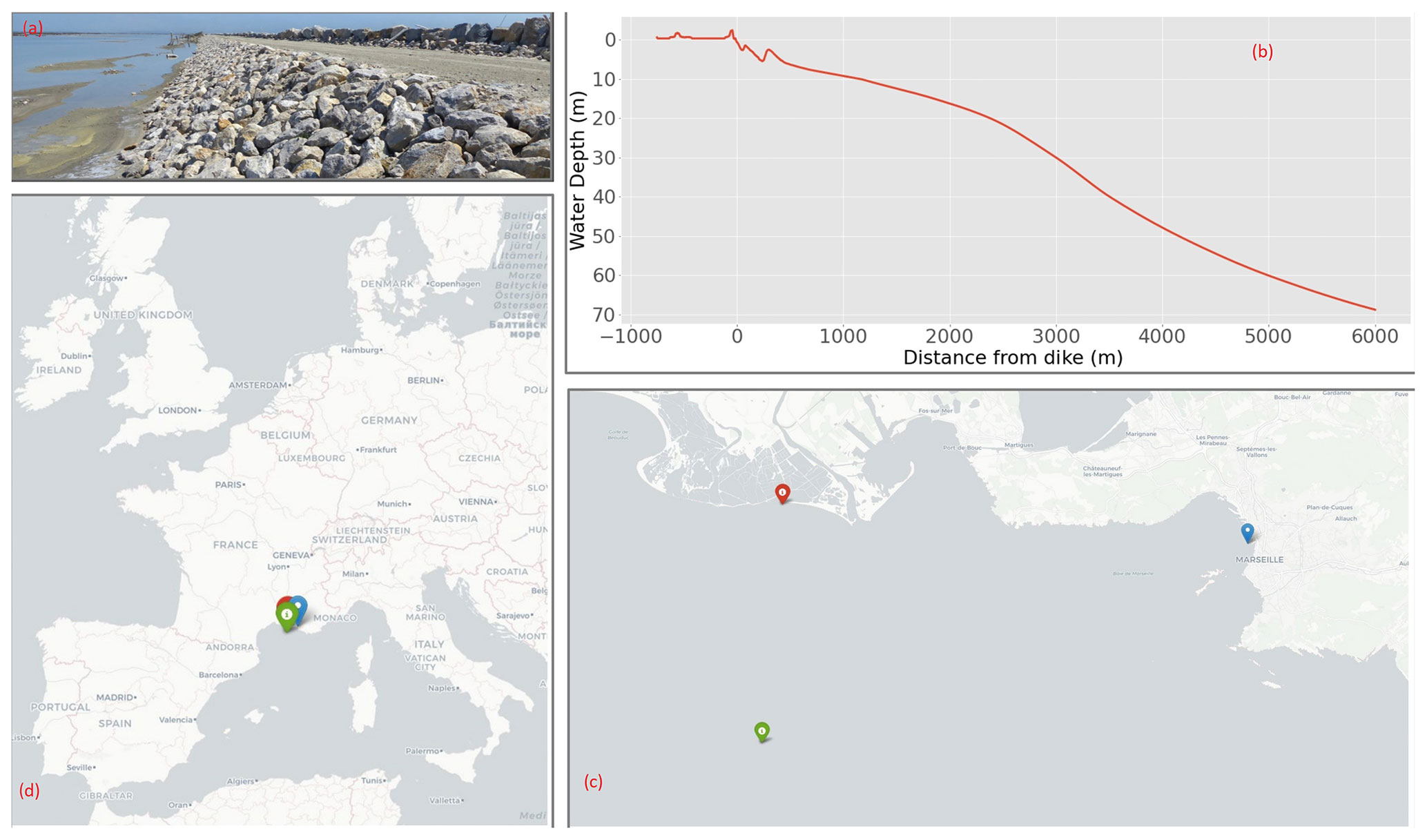
Figure 1(a) Picture of the landward slope of the dike made of sand and clay. (b) Water depth of the beach in front of the dike with resolution Δx=3 m. (c) Regional map of western Europe with the location of the dike (red), deepwater wave gauge (green), and sea level records (blue). (d) Regional location of the data sources.
The erosion problem of the dike is common in this area, and therefore assessment of erosion is necessary. The semi-empirical approach based on hydraulic loading has been well established and traditionally used. Wave propagation from deep water to the surf zone has been well explored both analytically, numerically, and experimentally in the literature. A large overview of the theory surrounding random sea wave propagation theory was provided by Goda (2000) and they brought advice on coastal protection. An evaluation of the different available methods on the subject has also been given by Liu and Han (2017). The complex nature of the overtopping phenomena makes it more difficult to model using only simple equations. Thus, many large-scale experiments have been conducted to deduce empirical laws as done by van der Meer (2011) as well as Hughes and Nadal (2008); Hughes et al. (2012) with the use of the wave overtopping simulator. Numerical simulations have also been explored by Li et al. (2003) using the volume of fluid method. More recently, the EurOtop manual (van der Meer et al., 2018) laid an extensive set of recommendations and experimentally based equations in order to functionally model the overtopping phenomenon. Bergeijk et al. (2019) also provided a more refined analytical model of overtopping using a set of coupled equations validated by numerical simulations and experiments.
Regarding the statistical tool to predict a higher risk, the copula theory has been well accepted and used to calculate multivariate return periods of natural hazards. De Michele et al. (2007) and Bernardara et al. (2014) wrote extensively on the subject with guidelines on using copulas to predict storm surges. More specifically, Kole et al. (2007) found that the Student's and Gumbel copulas are particularly interesting for risk management applications. Liu and Han (2017) deemed that the Clayton and Gumbel copulas are to be preferred for calculating multivariate joint return periods of natural hazards. Many methods are currently in use when estimating the probability of storm surges from sea states such as numerical models (SWAN or SWASH for example) as well as models based on wave energy. However, a more statistical approach based on bivariate copulas combining wave height and sea elevation are also widely used, as they are reliable and computationally inexpensive as seen in Salvadori and Michele (2007), but Orcel et al. (2021) expanded the method to trivariate copulas, allowing the method to yield the probability of structural failure. As indicated by many sources, we have a large choice of different copulas to link our different deep water conditions (Durante and Sempi, 2010, 2016; Tootoonchi et al., 2022). Among them, the Gumbel–Hougaard copula is commonly used to link the still water level to the wave height as done by Wahl et al. (2010) and Chini and Stansby (2006). As mentioned by Orcel et al. (2021), this will lead to the calculation of an “and” return period, yielding the expected mean time between two events where all metrics overreach a certain level (as opposed to an “or” return period where only one metric needs to overreach). However, there is very little research on the assessment of erosion of dikes combining statistical and probability approaches and theoretical and semi-empirical approaches as well. Mehrabani and Chen (2015) worked on a joint probabilistic approach for the assessment of climate change's effect on hydraulic loading. However, the authors constrained themselves to the frame of copula theory, assessing the risk to offshore conditions. That approach has considered neither interaction with a dike nor propagation of deep water wave but rather physical erosion criteria to put together a threshold metric. In the present study, we used a global sensitivity analysis to assess the most important parameters in the framework as the ones that contribute to the most variance of the system, in order to provide self-improvement to the framework as well as recommendations to improve the resilience of the dike. Combining different approaches, a sensitivity analysis, a fully functional and modular overtopping framework, and copula theory into a full stack has not been explored before and might provide useful guidance for the practitioner. Most works that laid the foundation for the last EurOtop manual (van der Meer et al., 2018) predict wave behavior up to overtopping but do not go further than this point. The focal point of such a study is often led by damages to infrastructure laid behind the dike, so the aforementioned limitations made sense. However, providing this extra step allows for quantification of the erosion damages provoked on the dike itself, which is the main focus here, as salt marshes do not bear costly infrastructure to protect. Also, erosion damage is often easier to observe and quantify than the overtopping phenomenon, which is quick, volatile, and difficult to measure on-site. Section 2 will describe the data used in the study. Section 3 will be focused on the methodology of the article, the most important equations regarding both the physical wave process, and the statistical processes. Results are presented in Sect. 4, followed by discussions on the advantages and shortcomings of the study as well as future potential improvements in Sect. 5.
The statistical study of coastal events requires relatively large, well documented, and high-quality datasets. Such historical data are not easy to find even in an area containing a dense network of coastal sensors. As a unified database of all records regarding offshore and coastal characteristics does not exist, we used data coming from different bases which contained the measures of interest with correct time synchronicity. We present the data in this section.
2.1 Bathymetry
We have at our disposal the bathymetry of the dike up to the deepwater point provided by the SHOM (Service Hydrographique et Océanographique de la Marine). The survey has a resolution of 3 m and spans over 6 km. As the distance from the dike to the ANEMOC (Atlas Numérique d'Etats de mer Océanique et Côtier) point (Fig. 1) is greater than 6 km, we use all the available data to calculate the mean slope of the beach in front of the dike.
2.2 Sea level records
As there is no sensor that recorded the sea level in the immediate vicinity of the dike, which would be highly sensitive to waves anyway, we had to resort to the nearest gauge that had a large record of measures, which was located in Marseilles's harbor (Fig. 1). The data of the gauge are maintained by the SHOM (https://data.shom.fr/, last access: 15 February 2023) in the REFMAR (Réseaux de rEFérence des observations MARégraphiques) database, which is part of the Global Sea Level Observing System (https://gloss-sealevel.org/, last access: 12 March 2023; GLOSS) and provides more than 100 years of hourly water elevation level. The acquisition is done using a permanent global navigation satellite system (GNSS) station. The place being located inside a port is protected from sea waves. It is located kilometers away from the actual site, but we will use these values as no on-site data are available currently. With the sea level being forced by atmospheric, mainly wind, conditions, non-linear effects are to be expected between sites, even when the tide gauges are relatively close. This underlines the importance of using on-site data whenever possible. The other issue would be the desynchronization of the data which are accounted for by our peak value selection method.
2.3 Significant wave height records
In situ data of the significant wave height provided at an hourly rate are difficult to find reliably over a long period of time (decades). This means that we have to resort to data provided by a numerical model. We use the data extracted from the ANEMOC-2 (https://candhis.cerema.fr/, last access: 10 August 2023) database currently maintained by the CEREMA (https://www.cerema.fr/fr, last access: 1 November 2022), reproducing numerically the sea conditions over a long period of time (from 1980 to 2010). The data are generated using the third generation of the spectral TOMAWAC (TELEMAC-based Operational Model Addressing Wave Action Computation), which is a part of the TELEMAC-MASCARET software suite. This model is used to interpolate sea states on many points calibrated using the GlobalWave in situ data. The significant wave height is estimated by calculating the mean value of the upper third of the recorded waves every hour. Thus, one value is given hourly at each chosen location. We have selected point 3667 (Fig. 1), as it is located in front of the dike and where the water depth is high enough to be considered as offshore (≈80 m) as the continental shelf has been reached according to bathymetry maps. It should be noted that model data carry an intrinsic uncertainty compared to experimental data, which is bound to decrease the reliability of the study.
2.4 Identifying storm surges and coupling the datasets
The time series data themselves are not directly exploitable, as the copula that we want to generate is based on the identification of extreme events implying a locally high value of both N and H0. We have many methods at our disposal to select extreme events, among which the peak-over-threshold is supposed to give the best results. However, selecting values over a certain peak gives a distribution bounded by the value of the threshold, which is not adapted to generate a full copula that can be used to calculate the return period of critical events (see Eqs. 12–14). Thus, we decided to use the block maxima approach, which gives good results and asymptotically converges to the generalized extreme value (GEV) distribution that we will use to fit the resulting data.
The choice of the block size is not obvious, as a small block size decreases the accuracy of the fit to the limit distribution (GEV), leading to a bias, but a large block size reduces the size of the sample, increasing the variance. The general approach is to consider the duration of the cycles between events. The seasonality of storm cycles and the requirement of independence between events would not allow us to use a value lower than 1 year, which is the block size we chose. This limited the size of our dataset significantly, meaning that more data would probably greatly improve our analysis.
As a preliminary check, correlation coefficients have been calculated to determine the relationship between the datasets. Pearson's coefficient gave ≈0.6, indicating a strong positive relationship. However, Pearson's coefficient is only applicable for linear correlations, which is unlikely, and is inappropriate for capturing outlier influence, making it artificially high. Kendall's and Spearman's coefficients are more appropriate in this case and gave ≈0.065 (with a p value of 0.002) and ≈0.095 (with a p value of 0.003), respectively. These values indicate a weak correlation, which indicates the dependency structure might not be captured by the indices and instead calls for another approach, based on copulas.
3.1 Multivariate statistical theory using copulas
The copula method is a popular approach for estimating return periods of extreme events in hydrology or finance and is commonly used as a tool of risk management, as univariate statistical analysis might not be enough to provide reliable probabilities with correlated variables as stated by Chebana and Ouarda (2011). One key advantage of the copula method over other methods is that it allows more flexible modeling of the dependence structure between variables. Other methods, such as the traditional joint probability method or the design storm method, assume a specific type of dependence structure (e.g., independence or fixed correlation), which may not accurately reflect the true relationship between the variables. In addition, the copula method can provide more accurate estimates of extreme events and their return periods, especially for events with very low probabilities of occurrence. This is because the copula method allows for a more precise estimation of the tail dependence between variables, which is important for accurately estimating extreme events. As we are looking for rather rare events in this study, this represents a considerable advantage. It however appears that the practitioner has a large selection of copulas to choose from depending on the nature of the data. The choice of which copula to choose varies from the type of data as well as the physics of the setup and even so we are left with a rather large selection. Merging multiple copulas in order to combine their properties has also been explored by Hu (2006), complicating the decision process further. Wahl et al. (2010) suggested that the Gumbel–Hougaard copula was particularly adapted when combining water level and wave intensity, although they used the time integral of the wave height over a threshold instead of the significant wave height, and the region of interest was the North Sea. Orcel et al. (2021) also recommended using the Gumbel–Hougaard or Clayton copulas for coastal waves on the Atlantic shores of France. An application of the Gumbel–Hougaard copula has also been explored on UK shores, aiming to study extreme coastal waves by Chini and Stansby (2006). This motivates us to directly use the Gumbel–Hougaard copula as the most adapted choice (Eq. 1).
where u and v are the cumulative distribution functions of the histograms originating from the datasets. The copula parameter θ represents the interdependency of the data.
The value of this copula parameter is important and can be calculated using a panel of different methods, i.e., the error method (see Appendix B for the equation as written by Capel, 2020) and the maximum-likelihood method.
Once done, the copula can be calculated using Eq. (1), attributing a probability of occurrence of any event E with one of the variables having a value smaller or equal to the defined ones, written as . The logical inverse can then be obtained by calculating the survival copula , defined as
Finally, we can associate each value of to a return period using the formula provided in Salvadori and Michele (2007):
where μ is the average interarrival time between two events of interest, i.e., the storms. The offshore conditions have been determined by a couple (N,H), the water level, and the significant wave height, respectively, with an associated return period. This gives us the properties of an offshore wave.
3.2 Maximum-likelihood method
The principle of the maximum-likelihood method that we use is that we try to maximize the function L in Eq. (4), yielding the likelihood of generating the observed data for a set value of θ. It essentially means that, given a set of data, a high value of L indicates that the function is highly likely to have been able to generate the data sample.
where cθ is the copula density, which can be obtained by calculating the derivative of the copula function with respect to its cumulative density functions in Eq. (5):
3.3 Wave theory: from offshore to the critical velocity
We are able to link a deep water state to a return period. However, this does not give us any information on the probability of the occurrence of an event that would provoke erosion. Hence, we need to assess what kind of event provokes erosion using Eqs. (6)–(11) to calculate the terminal velocity of the flow on the landward slope.
3.3.1 Propagation
The offshore significant wave height can be propagated up to the toe of the dike. Among the numerous methods, the most convenient one to use is the propagation formula written in Eq. (6), extracted from Goda (2000), allowing us to calculate the significant wave height at the toe of the dike Hm0, which is the mean of the third of the highest wave heights over a set period of time, as follows. This metric is important, as it is bound to be used for future calculations of the overtopping characteristics. Note that refraction is neglected in our case:
where H0 is the offshore wave height. Ks is the shoaling coefficient, d is the water depth at the toe of the dike, and L0 is the deepwater wavelength. The coefficients β0, β1, and βmax can be calculated as detailed in Goda (2000)1.
3.3.2 Overtopping equations
Once the wave reaches the toe of the dike, the wave will start interacting with the dike in what is called the overtopping phase. This phenomenon is divided into 3 steps, with the equations detailed in van der Meer et al. (2018). We give a brief summary here of the used equations.
-
Run-up. The wave reaches the dike and flows up towards the crest. The run-up height reached by 2 % of the incoming waves is calculated (Eq. 7).
where ξ is the Iribarren number, and Hm0 is the wave height at the toe of the dike. The γ factors γb, γf, and γβ yield the contribution of the berm, the roughness and porosity of the seaward slope, and the obliquity of the waves, respectively.
-
Crest flow. The water flows on the crest up to the landward slope. We calculate the flow velocity (Eq. 8) and thickness (Eq. 9) at the beginning of the crest using the previously calculated run-up height.
with cv2 % and ch2 % representing arbitrary coefficients that are used as fitting parameters. zA is the height of the dike above the still water level and g the gravitational acceleration. These equations were compiled in van der Meer (2011) and van der Meer et al. (2012) from the works led by Shüttrumpf and van Gent (2003) and Lorke et al. (2012).
The flow velocity will then decay along the crest (Eq. 10) as a function of distance from the seaward side of the crest (xc). It is important to note that this formula is only valid for a few meters long crests, as the formula becomes less precise for higher values of xc.
with representing the deep water wavelength of the incoming waves.
According to van der Meer et al. (2012), the decrease of flow thickness upon reaching the crest is about one-third and can be attributed to the change of direction of the flow, staying relatively constant along the crest.
-
Landward slope flow. The water trickles down the landward slope; this is where erosion usually happens. Terminal velocity (Eq. 11) is quickly reached on such slopes, so we can use this formula directly instead of the landward flow velocity.
where hb0 and vb0 are the flow thickness and velocity at the entry of the slope, respectively. f is the friction coefficient, which is determined experimentally whenever possible (an estimation can be used instead if experiments are unavailable), g the gravity acceleration, and β the slope angle.
These equations rely on a large number of parameters that are detailed in the table below.
van der Meer et al. (2018)Hughes et al. (2012)Goda (2000)Goda (2000)Table 1Main control parameters in the equation system of the framework with their reference value and their interval of variation for the GSA (global sensitivity analysis).
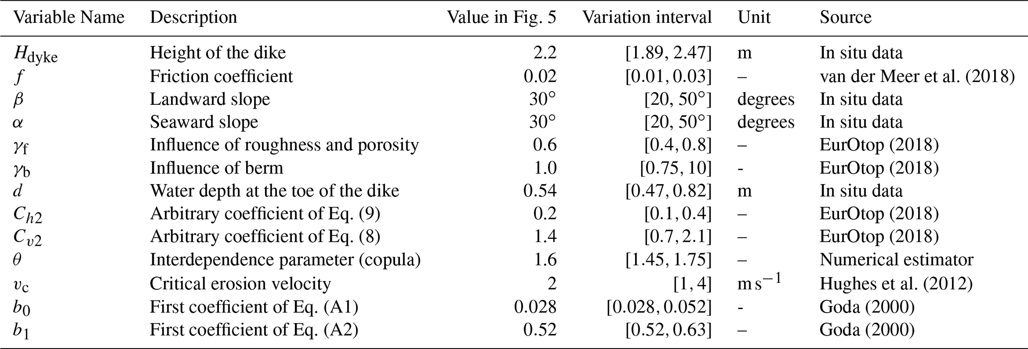
Defining the value of these parameters is not easy, and they may carry some amount of uncertainty that needs to be quantified. We propose a sensitivity analysis to resolve this problem.
3.4 Return period of soil erosion
We can now associate a terminal velocity with a set that is the set of couples (N,H0) through the function f to a terminal velocity vt.
By integrating the derivative of the copula with respect to H0 along the isoline 𝒮vt, we can obtain the return period of event , which is any event implying a terminal velocity equal or higher than vt (see Eqs. 12 to 14).
where C is the surface of integration, which is the area above the velocity curve, and S(H0) the velocity curve. This means that we can calculate the return period associated with a certain terminal velocity threshold for a defined dike by fixing the parameters in Table 1. We give reference values to these parameters. They are obtained either experimentally from in situ data or extracted from the literature when observations are unavailable. The details of the values are explained in Sect. 3.5.1.
3.5 Sensitivity analysis through the Quasi-Monte-Carlo process
3.5.1 Uncertainty parameters
The showcased system is indeed able to provide return periods associated with events leading to erosion or any dangerous event defined as a criteria on flow velocity. However, added to the deep water conditions used to generate the copula are the characteristics associated with the dike, as well as many empirical parameters used to fit the laws allowing the calculations leading to the landward terminal velocity of the dike. All of these parameters carry an intrinsic amount of uncertainty which has a non-negligible impact on the results. This calls for an accurate quantification of the whole potential range of variation of each parameter. A global sensitivity analysis through the computation of global sensitivity indices will be our tool of choice. A combination of the first-order and total effect sensitivity indices (Eqs. 17–18) is a principled and classical approach that encapsulates a useful enough amount of information on the variation of the system's characteristics.
We estimate the value of the indices using the Saltelli estimator defined in Saltelli et al. (2008). With the number of dimensions being high, we accelerate the convergence of the estimator using a pseudo-random sampler, in our case the Sobol' sequence, which generates a low discrepancy sample of points. The resulting distribution of the parameters is thus uniform, which is standard for the Monte-Carlo method. The performance comparison of the Monte-Carlo process against the improved Quasi-Monte-Carlo estimations has been extensively discussed, noticeably in Sobol' (1990, 1998), Sobol' and Kucherenko (2005), and Acworth et al. (1998). The improvement in performance is unanimously in favor of the Quasi-Monte-Carlo Method.
The first step is to define the parameters used in Eqs. (1)–(11) that we are going to consider as relevant sources of uncertainty. They are compiled into Table 1, where we associate a potential range of variation that is deemed as reasonable with its source. Each parameter is further described in its associated description below. We also provide a brief description of the parameters, as well as the estimation technique.
-
The height of the dike. Hdyke is defined as the vertical distance between the still water level in a calm sea condition and the culminating point of the dike. Using in situ data from a Litto3D bathymetry map, we managed to obtain the distribution of the dike height. We use the mean of the heights as the reference value (Table 1) and give an interval of variation that is approximated by the standard deviation for sensitivity analysis. The same procedure is done for the geometrical parameters α, β, and d.
-
The friction coefficient. f yields the resistance of contact between two materials, in our case between the landward slope of the dike and water. A higher coefficient brings a slower flow velocity but also more shear stress. Different values can be used here. It is generally considered that for smooth surfaces and vegetation a value close to 0.02 can be used. We assume that is it possible to use such a value for small rocks with a diameter of approximately 20 cm, which is what is currently implemented on the Quenin dike.
-
The landward slope. β is defined from the end of the crest which is considered as flat. The steeper the slope is, the higher the terminal velocity. It should be noted that a combination of high crest velocity and steep landward slope can provoke a flow separation at the end of the crest followed by an impact on the slope, resulting in added normal stresses. This behavior may be significant and has been explored by Ponsioen et al. (2011).
-
The seaward slope. α is defined as the mean slope from the toe of the dike to the beginning of the crest, assuming that the crest is flat. Its value is important, as the behavior of the up-rushing wave may change drastically for different values of α.
-
The influence of roughness and porosity. Roughness and porosity influence on the seaward slope γf is a factor with a value ranging from 0 to 1, scaling how much the run-up will be attenuated thanks to the slope surface characteristics (1 means no influence). This is difficult to estimate, as it relies on in situ experiments. Evaluating this parameter is not easy. Hence, we chose a relatively large range of variation around the reference value, as the rocks on the slope are expected to have an influence of the same order of magnitude as other structures described in the EurOtop.
-
The influence of the berm. γb, with a value between 0 and 1 indicates the attenuation of the wave due to the presence of a berm. This value can be estimated using the geometry of the dike if it is simple. It is more uncertain for a more complicated geometry. We calculate this factor using equations given in the EurOtop. The dike is heterogeneous through its length, and its geometry is more complicated than what is used for the calculation as it is a natural berm. Thus, we gave it some variability, deciding that it could not result in more than 25 % water height reduction, which is already dramatic.
-
The depth at the toe of the dike. b is calculated in situ using the Litto3D map as previously cited. Its value is registered for every transversal cross-section of the dike.
-
The scaling coefficients of the input crest velocity and thickness. Ch2 and Cv2, respectively, are scaling factors on the equations calculating the velocity and thickness of the flow at the beginning of the crest from the run-up. The range is estimated as a variation of ±50 % from their suggested values in the EurOtop (2018).
-
The correlation parameter. θ determines the intensity of the correlation between the datasets. The results obtained from the maximum-likelihood estimation (MLE) suggest that a small plateau is located around the maximum value, so a 10 % variation interval is a reasonable assumption here.
3.5.2 Sobol' indices
If we provide our framework inputs that are uncertain, it should be expected that the uncertainty will be carried through the system up to the outputs. We rely on sensitivity analyses to quantify such uncertainty by comparing the influence of each parameter on the variation of the outputs relative to their respective range of variation. Since there may be a lot of interaction between parameters and we need to assess the influence of the parameters over their whole range of variation, we use a global sensitivity analysis.
Let be a function of the Xi parameters, with . The uncertainty of the parameters Xi will carry over the uncertainty of the output Y. Therefore, it would be necessary to estimate the impact of parameters on the output Y.
In order to quantify the influence of a single parameter Xi on a complex system, a good starting point can be to fix this parameter to a defined value xi. Logically, freezing a parameter, which is a potential source of variation, should reduce the variance V(Y) of the output Y. Hence, a small value of variance would imply a high influence of the parameter Xi. We can globalize the approach by calculating the average value of the variance over all valid values of xi, preventing the dependence on xi. This is written as
The following relation is also useful in our case:
The conditional variance is called the first-order effect of Xi on Y. We can then use the sensitivity measure called the sensitivity index or Sobol' index (see Sobol, 2001), defined as
This gives the proportion of contribution of the parameter Xi alone on the total variance of the output Y relatively to the other parameters X∼i. The main drawback of this measure is that the interaction of the parameters between themselves is not taken into account. These measures are contained in higher-order indices. However, this may become quite time consuming and impractical if the number of parameters is high, as the total number of Sobol' indices that could be calculated grows as n!, with n representing the number of parameters.
The total effect Sobol' index, which measures the influence of a parameter i on the variance as well as its interaction with every other parameter, is calculated following the same method, but instead of freezing parameter i, we freeze every other parameter j≠i (Eq. 18).
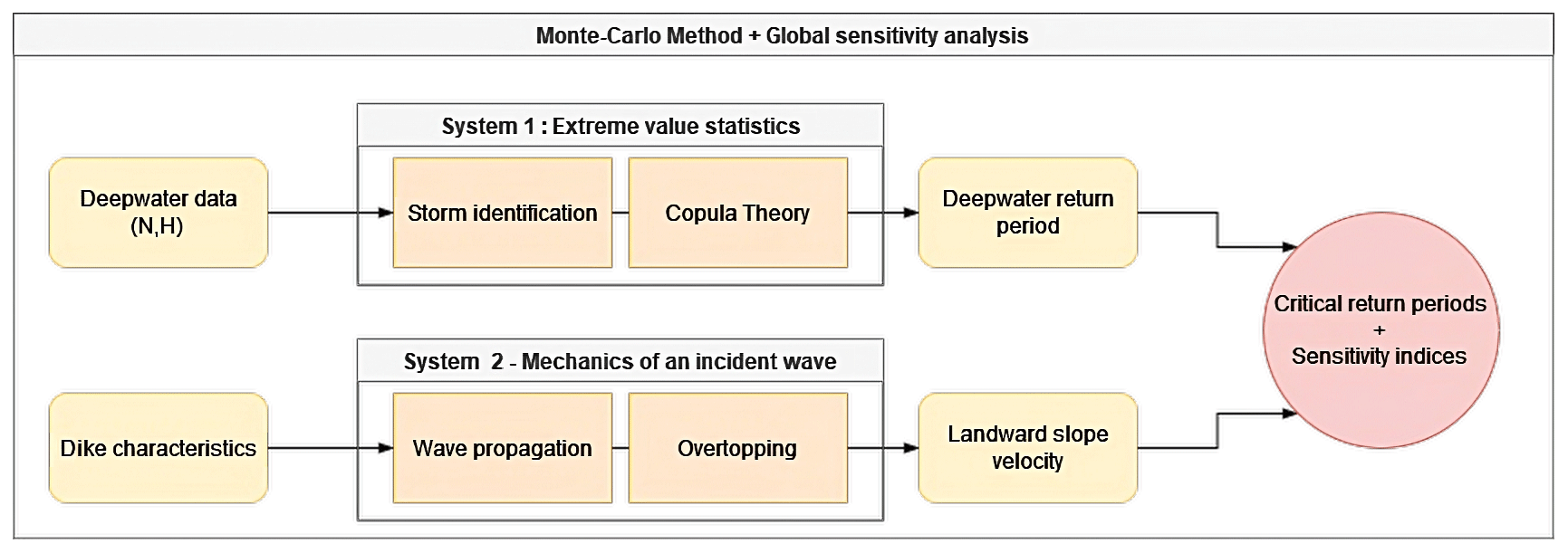
Although concise, the Eqs. (17)–(18) are difficult to calculate analytically. We circumvent the problem by using the method developed by Sobol (2001) and further improved by Saltelli et al. (2008). The protocol can be summarized as follows (Fig. 2):
-
define the input parameter space and the model output function;
-
generate a set of samples using Latin hypercube sampling (LHS) or another quasi-random sampling method (we used Sobol' sequence in our case);
-
compute the model output for each set of input parameters;
-
partition the output variance into components due to individual input variables and their interactions using an ANOVA-based decomposition;
-
calculate the first-order and total effect Sobol' indices, which measure the contribution of individual input variables and their interactions to the output variance, respectively.
The procedure can be summarized as a dual process of using statistics, with copula theory to generate a copula associating return periods to a couple (N,H) of deepwater metrics on one side and calculating the interaction of the same couple (N,H) with the dike to calculate the landward slope velocity on the other side. This whole chain can then be inputted into a global sensitivity analysis method (Fig. 2).
4.1 Return period copula
We start by compiling the selected storm surge events into a histogram, giving the univariate probability densities of both datasets. However, since we only work with about 20 years of hourly data, we need to fit the cumulative histogram in order to create a cumulative distribution function that allows us to extrapolate to rarer events. We use the generalized extreme value distribution, which is used for the estimation of tail risks and is currently applied in hydrology for rainfalls and river discharges in the context of extreme events as in Muraleedharan et al. (2011).
This means that the events can then be sorted into a histogram for us to observe their respective univariate distributions. In this case, the sample limits us to events that can happen up to once every 20 years, since we have no data covering a larger period. Thus, we can obtain information about more extreme events by extrapolating the data using a fitted distribution on each individual sample. Using the block maxima event selection, the Fisher–Tippett–Gnedenko Theorem indicates that extreme values selected this way asymptotically follow the generalized extreme value distribution (GEV) (Eq. 19), which we use to fit the data. The distribution is described here:
with ) representing the location, scale, and shape factor, respectively. The results are displayed in Fig. 3. The laws are fitted using the maximum-likelihood method. The fit gives a R2 score higher than 0.999 for both datasets. Hence, we consider the fit almost perfect, and it will not be accounted for during future calculations of uncertainty, as it is considered insignificant compared to other sources.
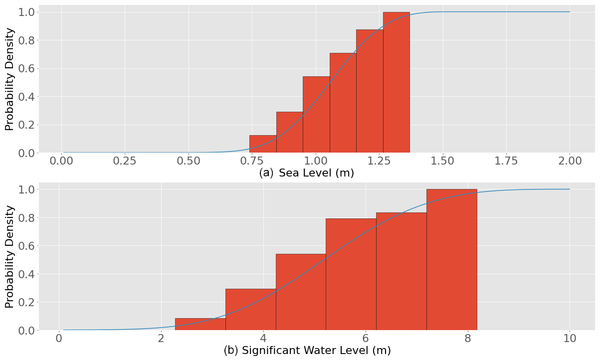
Figure 3Cumulative distribution functions of the offshore significant wave height (a) and the still water level (b) displayed in a histogram. They are fitted to the GEV distribution with good concordance.
We will then compute the derivative of the copula in Eq. (1) and maximize the value of L(θ) from Eq. (4).
The interdependence parameter can take values in the interval , where 1 is the independent copula, and +∞ means absolute correlation. A value of 1.23 means that there is a moderate correlation between the two distributions. This can be seen visually in Fig. 4, as the contour lines form an L shape, indicating that the values are strongly linked. Hence, we can generate the copula using Eq. (1). The cumulative distribution function yields the probability of a value laying under a threshold. Hence, we use Eq. (2) to inverse the copula and obtain the survival copula (Fig. 4). This allows us to evaluate the return period of any event E so that using Eqs. (1–3).
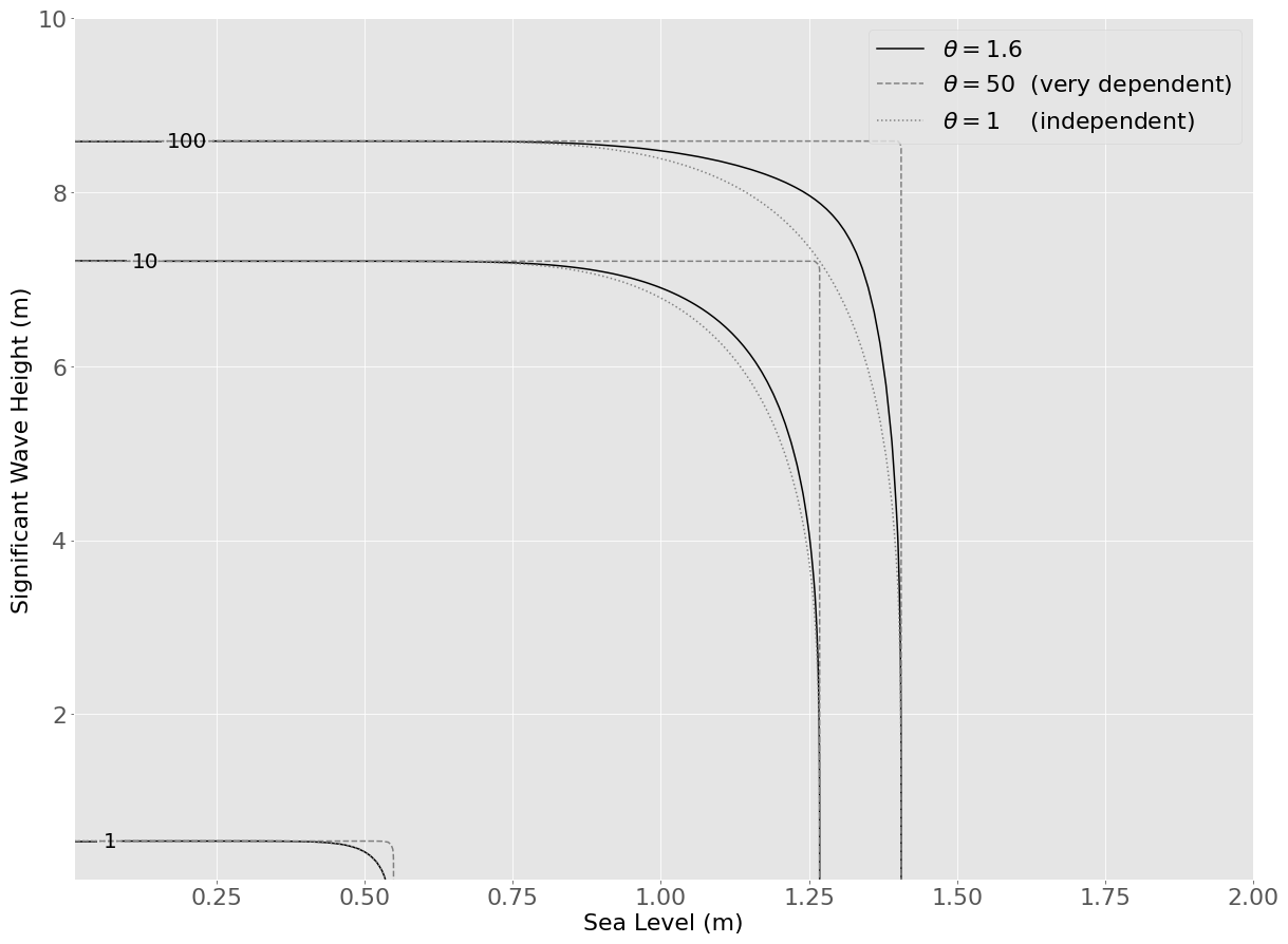
Figure 4Return period (in years on the contour lines) of an event composed of a couple (N,H0) or with a higher value of N or H0, noted as with the interdependence factor having a value of θ≈1.23 (full line). The independent copula (dotted lines) and the high-dependence copula (dashed lines) are also displayed for reference.
The contour lines of the copula in Fig. 4 show that the data are coupled to some degree. Indeed, since the data are correlated, a high value of the water level N and the significant wave height H should be more probable than if the data were uncorrelated, thus decreasing the return period and driving the contour lines toward the smaller values.
4.2 Computing the terminal velocity
We use the terminal velocity on the landward slope vt as a criterion of erosion. This means that damage starts to occur when vt>vc, where vc is the critical velocity which has to be determined using the literature. Using Eqs. (6)–(11), we can calculate it from any couple (N, H0) of offshore water level and significant wave height, given that the mean slope of the bathymetry is known. The results are shown in Fig. 5.
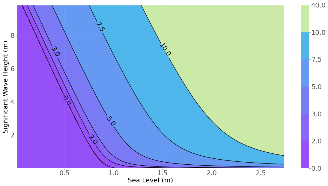
Figure 5Terminal velocity (in m s−1 on the contour lines) along the landward slope for any couple (N,H0). Higher sea level and significant wave height bring higher terminal velocity.
Unsurprisingly, higher values of both N or H0 induce higher values of terminal velocities. All values below the “0.0” line (Fig. 5) failed to produce overtopping and thus generate a null value while in fact there is no water flowing on the slope.
Typically, we observe that the Quenin dike's landward slope is covered by rubble mounds which have an average diameter of 20 cm. Applying Peterka's formula (Peterka, 1958) (Eq. 20), which is used by the U.S. Bureau of Reclamation, we can obtain the critical velocity of erosion on the dike.
where v* is the critical erosion velocity, and d50 is the median block parameter. For blocks with a diameter of 20 cm, we obtain a critical erosion velocity of approximately 2 m s−1. Our calculations estimate that such flow velocity will occur on average once every 5.86 years. This gives a higher value than what is reported by the Salins du Midi company, currently exploiting the dike. The company reports significant damage that needs to be repaired approximately once every 2 years. This has been confirmed by its archives. This gap can be caused by uncertainty on the parameters which will be further estimated via sensitivity analysis.
4.3 Sensitivity indices
After generating a sample of parameter values, each set is computed through the framework, giving an associated return period from which we calculate the global sensitivity indices of both first order and total effect (Fig. 6).
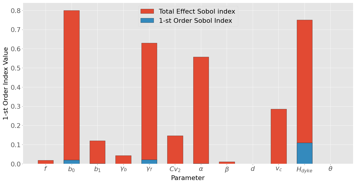
Figure 6Value of the first-order sensitivity (in red) and total effect (in blue) indices for each tested parameter.
A few observations can be made about the results. It appears that there is some correlation between the first-order Sobol' index and the total effect index. This is not surprising, as the total effect index encapsulates all orders, including the first order. However, many parameters showing a value close to zero at first order had much higher values on the total effect index. It is safe to assume that the other parameters presenting a high total effect value likely show some uncertainty when interacting with the three parameters and thus that the first-order index is clearly not sufficient. Then, the considered parameters contribute very differently to the uncertainty of the system. It is essential to remind one that high contribution to uncertainty can mean either that the parameter is very influential or that it is very uncertain (or both). We will focus on the three main parameters showing both high first-order and total effect values.
-
γf. This parameter intervenes at the beginning of the overtopping process and thus should present a high degree of interactivity with other parameters, which explains the very high total effect index value. The parameter is undoubtedly very influential, since it is a direct coefficient of the overtopping wave height. However, this parameter is very difficult to assess experimentally, and we had to rely on reference values for the variation interval. This means that a part of the uncertainty can be explained by a large range of variation defined in the bound of the global sensitivity analysis. This result is corroborated by de Moel et al. (2012), where they proceed similarly and find that the majority of the uncertainty is held by the overtopping process.
-
Hdyke. The dike height is one of the most important parameters considered when designing a dike, so observing high Sobol' indices values is not a surprise. Furthermore, the in situ data showed that the dike was not homogeneous, with height varying between 1.7 and 2.5 m. This could be a problem, as it reveals the presence of weak points on the dike where damage could occur, showing the limit of working with reference values. Hence, improving the dike by making it more homogeneous could reduce the uncertainty of the system.
-
b0. This parameter is involved with wave propagation from offshore to the toe of the dike. It intervenes early in the process and therefore can have some influence on the other parameters. The reference value of b0 was originally defined by Goda (2000) using in situ experiments. The range of variation chosen may have been artificially large, but using numerical models would bring great improvements to the system uncertainty.
Most of the important parameters are strongly linked to geometrical features of the dike, highlighting the importance of good characterization of the physical parameters of the dike through experiments and design in order to reduce the intervals of variations and thus the uncertainty. It also underlines the homogeneity of dike construction as one of the main concerns of future dike designs. It finally appears that all processes seem to contribute to the global uncertainty of the system, only the statistical part seems to be insignificant.
4.4 Return period distribution
Launching such a high number of calculations allows us to compile the return periods into a histogram to evaluate the probability of the return periods taking into account uncertainties. The results are compiled in Fig. 7.
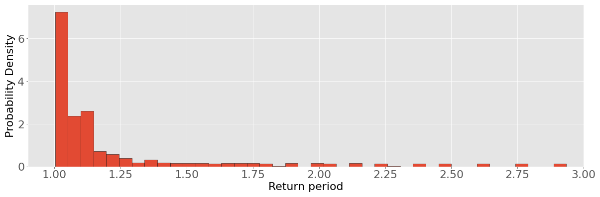
Figure 7Distribution of the return periods of an event able to provoke some amount of erosion to landward slope at the dike, with random variation of the parameters in Table 1 according to their respective range of variation. The distribution is truncated for clarity, but some very rare outliers reached values up to 3000 years.
The distribution of values appears to form a cluster close the 1-year mark, with many outliers showing very high values. Note that for clarity purpose the histogram has been truncated, but values range from 0 up to 3000 years. With the mean value being biased because of the very high values of the return periods, the median is a more appropriate metric, which gave a value of ≈1.1 years. This value is very close the in situ observation at the Quenin dike relayed by the operator and comforts us in the reliability of our current analysis.
5.1 Results validation
In order to make sure that the estimation of the sensitivity indices is accurate, we need to ensure that the convergence of the estimator has been reached. We will do this by plotting the values of the indices and incrementally increasing the number of points generated by the Sobol' sequence; this is called a validation curve. Note that the number of plotting points is limited because the Sobol' sequence, being a non independent sample, is only valid for 2n points. The results are displayed in Fig. 8.
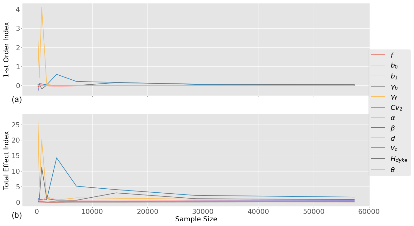
Figure 8Evolution of the values of the first-order sensitivity index (a) and total effect sensitivity index (b) with sample size.
Convergence has evidently been reached. It seems that we can safely use ≈40 000 points which in our case is still fairly low as the computation of the terminal velocity is pretty fast. However, should the computation time increase by changing the methods of calculation, this could become a problem which would require more intensive optimizations.
5.2 Good practices and dike improvements
Results from the global sensitivity analysis give indications on how the dike could be reinforced in order to increase the most the return periods. The recommendation would be to act upon the most significant parameters of the analysis, meaning the ones which yield the highest values of Sobol' indices. This indicates that the geometrical features of the dike, the crest height as well as the slopes, should be acted upon first whenever possible. Elevating the dike or decreasing its seaward steepness should bring good results, while altering the erosion properties of the landward slope does not look so promising. This focus on the geometrical features of the dike is supported by Sibley et al. (2017). Generally, the recommendations of the USACE (United States Army Corps of Engineering) seem to focus mainly on geometrical features and secondly on erosion resistance when considering the design of levees. Approaching the problem using Sobol' indices in this particular use case had not been done before and seems to provide similar results, confirming the value of the method. The recommendations stated here do not include, however, an analysis of cost-effectiveness, which should be one of the next milestones of the work that is presented here.
5.3 Limits of the study
The framework provides a rather complete approach but obviously suffers some limitations. Some of them are inherent to the system itself, while others call for future improvements. Our main focus was to obtain an assessment of the risk of erosion on the landward slope of the dike. Coastal protection is nonetheless submitted to many other damages such as erosion in other locations like the crest of the seaward slope. A more general criterion of security such as “any damage to the dike” would require one to broaden the calculations to take all possible damages into account. We have also limited our criteria of interest as a condition of whether or not the critical velocity has been overreached on the landward slope. The possibility of a breach or the actual amount of eroded material is therefore not quantified. For practical reasons, we calculated return periods on an averaged profile of the dike, which as stated by the global sensitivity analysis can lead to a return period different from the local profile. A location-wise study could bring reduced uncertainty and bring more relevant results. The data sources used to make our analysis are incomplete, located in far away places, or generated using numerical models. It is necessary to use in situ data extracted from experimental devices in order to improve the reliability of the study. Moreover, the study uses long-term data, but the impact of climate change implies an elevation of the water level as well as changes in the characteristics of storm surges such as intensity, duration, or frequency. Integrating these effects should be done in the future in order to improve long-term studies. This problem is especially important for more resilient dikes dealing with higher return periods.
We have been able to build a complete automated framework allowing the user to estimate the expected return periods of events leading to erosion on the rear side of the earthen dike submitted to wave overtopping, assuming the correctly assessed ranges of variation of the parameters are provided. The framework itself needs, firstly, metocean data in order to create a reliable copula from wave and water level data, then a description of wave propagation to the toe of dike, and finally reliable laws representing wave overtopping process, run-off on the crest then on the landward slope, and bottom erosion.
The return period from which erosion on the Quenin dike located in Salin-de-Giraud starts is firstly estimated from reference parameters. This first estimate is equal to 6 years, which is significantly higher than the value of 2 years written in reports from the operating company. The framework is then able to take the parameters' uncertainty into account, which provides a generalized extreme value distribution of return periods which is right skewed with a peak around the 2 years value and a long tail in the upper range of the return periods. This result shows that a statistical study is necessary to determine a return period of damages in accordance with observed damages. Damages on a long dike are not observed on an average profile but on the weakest profile. That is why the peak of the statistical analysis is more representative than the first estimate based on average parameters. Sensitivity analysis is implemented into the framework and classifies the dike's parameters in terms of carried uncertainty. No clear trend can be observed for a specific category of parameter that would carry a significant part of the global uncertainty. However, the protocol allows us to clearly distinguish which parameters should be closely considered and which ones can be ignored. The results underline the importance of characterizing the dike using experiments and simulations in order to reduce the parameters' range of variation as much as possible. All processes contribute significantly to the uncertainty of the system, excluding the statistical treatment. This study case is indeed very specific, with a very low return period for damages and large variations of the dike crest. For any other dike, the framework is applicable by providing the appropriate input values.
Finally, the results can be provided relatively quickly without an enormous amount of computing power. They can indeed be validated using only a small set of points for the Quasi-Monte-Carlo process (around 15 000 points at most).
with m representing the average steepness of the seabed between the offshore point and the toe of the dike, θa the angle of attack of the oblique waves, and L0 the deep water wavelength. b0 and b1 are coefficients determined empirically from Goda (2000), who gives them values of 0.028 and 0.052, respectively.
The data are freely available on demand from the corresponding author. REFMAR is freely accessible by creating an account at http://data.shom.fr (last access: February 2023; https://doi.org/10.17183/REFMAR, SHOM, 2023). ANEMOC is accessible on demand by contacting the handler directly at anemoc.prel.drel.dtecrem.cerema@cerema.fr (last access: March 2023; license, Etalab open license; https://doi.org/10.5150/jngcgc.2014.013, Laugel et al., 2023).
CH – conceptualization, methodology, software, investigation, writing – original draft, data curation, visualization.
AP – supervision, writing – review and editing, methodology, resources.
PS – conceptualization, methodology, validation, surveillance, project administration, funding acquisition.
AB – conceptualization, supervision, project administration.
JJ - supervision, writing - review and editing, resources, funding acquisition, project administration.
The contact author has declared that none of the authors has any competing interests.
Publisher's note: Copernicus Publications remains neutral with regard to jurisdictional claims in published maps and institutional affiliations.
This article is part of the special issue “Hydro-meteorological extremes and hazards: vulnerability, risk, impacts, and mitigation”. It is a result of the European Geosciences Union General Assembly 2022, Vienna, Austria, 23–27 May 2022.
We hereby thank the Salins du Midi company for financially supporting the work and especially Pierre-Henri Trapy for providing useful information on the site, guidance, and access to the company's archives.
This paper was edited by Francesco Marra and reviewed by two anonymous referees.
Acworth, P., Broadie, M., and Glasserman, P.: A Comparison of Some Monte Carlo and Quasi Monte Carlo Techniques for Option Pricing, in: Monte Carlo and Quasi-Monte Carlo Methods 1996, edited by: Niederreiter, H., Hellekalek, P., Larcher, G., and Zinterhof, P., Lecture Notes in Statistics, Springer, New York, 127, https://doi.org/10.1007/978-1-4612-1690-2_1, 1998. a
Bergeijk, V. V., Warmink, J., van Gent, M., and Hulscher, S.: An analytical model of wave overtopping flow velocities on dike crests and landward slopes, Coastal Eng., 149, 28–38, 2019. a
Bernardara, P., Mazas, F., Kergadallan, X., and Hamm, L.: A two-step framework for over-threshold modelling of environmental extremes, Nat. Hazards Earth Syst. Sci., 14, 635–647, https://doi.org/10.5194/nhess-14-635-2014, 2014. a
Capel, A.: Wave run-up and overtopping reduction by block revetments with enhanced roughness, Coastal Eng., 104, 76–92, 2020. a
Chebana, F. and Ouarda, T.: Multivariate quantiles in hydrological frequency analysis, Environmetrics, 22, 63–78, 2011. a
Chini, N. and Stansby, P.: Extreme values of coastal wave overtopping accounting for climate change and sea level rise, Coastal Eng., 65, 27–37, 2006. a, b
De Michele, C., Salvadori, G., Passoni, G., and Vezzoli, R.: A multivariate model of sea storms using copulas, Coastal Eng., 54, 734–751, 2007. a
de Moel, H., Asselman, N. E. M., and Aerts, J. C. J. H.: Uncertainty and sensitivity analysis of coastal flood damage estimates in the west of the Netherlands, Nat. Hazards Earth Syst. Sci., 12, 1045–1058, https://doi.org/10.5194/nhess-12-1045-2012, 2012. a
Durante, F. and Sempi, C.: Copula Theory: An Introduction, Lecture Notes in Statistics, 198, 3–31, 2010. a
Durante, F. and Sempi, C.: Principles of Copula Theory, CRC Press, 2016. a
Goda, Y.: Random Seas and Design of Maritime Structures, vol. 15, World Scientific Publishing Co., https://doi.org/10.1142/7425, 2000. a, b, c, d, e, f, g
Hu, L.: Dependence patterns across financial markets: a mixed copula approach, Applied Finance Economics, 16, 717–729, 2006. a
Hughes, S. and Nadal, N.: Laboratory study of combined wave overtopping and storm surge overflow of a levee, Coastal Eng., 56, 244–259, 2008. a
Hughes, S., Thornton, C., der Meer, J. V., and Scholl, B.: Improvements in describing wave overtopping processes, Coastal Eng., 1, 35, 2012. a, b
Kole, E., Koedijk, K., and Verbeek, M.: Selecting copulas for risk management, Journal of Banking and Finance, 31, 2405–2423, 2007. a
Laugel, A., Tiberi-Wadier, A.-L., Benoit, M., and Mattarolo, G.: ANEMOC-2, PARALIA [data set], https://doi.org/10.5150/jngcgc.2014.013, last access: March 2023. a
Li, T., Troch, P., and Rouck, J. D.: Wave overtopping over a sea dike, J. Comput. Phys., 198, 686–726, 2003. a
Liu, S. and Han, J.: Energy efficient stochastic computing with Sobol sequences, Design, Automation & Test in Europe Conference & Exhibition, 2017, Lausanne, Switzerland, 650–653, https://doi.org/10.23919/DATE.2017.7927069, 2017. a, b
Lorke, S., Borschein, A., Schüttrumpf, H., and Pohl, R.: Influence of wind and current on wave run-up and wave overtopping, Final report., FlowDike-D, 2012. a
Mehrabani, M. and Chen, H.: Risk Assessment of Wave Overtopping of Sea Dykes Due to Changing Environments, Conference on Flood Risk Assessment, March 2014, Swansea University, Wales, UK, 2015. a
Muraleedharan, G., Soares, C. G., and Lucas, C.: Characteristic and Moment Generating Functions of Generalised Extreme Value Distribution (GEV), Sea Level Rise, Coastal Engineering, Shorelines and Tides (Oceanography and Ocean Engineering), 14, 269–276, 2011. a
Orcel, O., Sergent, P., and Ropert, F.: Trivariate copula to design coastal structures, Nat. Hazards Earth Syst. Sci., 21, 239–260, https://doi.org/10.5194/nhess-21-239-2021, 2021. a, b, c
Peterka, A.: Hydraulic design of stilling bassin and energy dissipators, Engineering Monograph, 25, 222, PB95139457, 1958. a
Ponsioen, L., Damme, M. V., and Hofland, B.: Relating grass failure on the landside slope to wave overtopping induced excess normal stresses, Coastal Eng., 14, 269–276, 2011. a
Pörtner, H.-O., Roberts, D., Tignor, M., Poloczanska, E., Mintenbeck, K., Alegría, A., Craig, M., Langsdorf, S., Löschke, S., Möller, V., Okem, A., and Rama, B. (Eds.): Climate Change 2022: Impacts, Adaptation, and Vulnerability. Contribution of Working Group II to the Sixth Assessment Report of the Intergovernmental Panel on Climate Change, Cambridge University Press, https://doi.org/10.1017/9781009325844, 2022. a
Saltelli, A., Ratto, M., Terry, A., Campolongo, F., Cariboni, J., Gatelli, D., Saisana, M., and Tarantola, S.: Global Sensitivity Analysis, The Primer, John Wiley and Sons, Ltd, https://doi.org/10.1002/9780470725184, 2008. a, b
Salvadori, G. and Michele, C. D.: On the use of Copulas in Hydrology: Theory and Practice, J. Hydrol. Eng., 12, 369–380, https://doi.org/10.1061/(ASCE)1084-0699(2007)12:4(369), 2007. a, b
Sergent, P., Prevot, G., Mattarolo, G., Brossard, J., Morel, G., Mar, F., Benoit, M., Ropert, F., Kergadallan, X., Trichet, J., and Mallet, P.: Stratégies d'adaptation des ouvrages de protection marine ou des modes d'occupation du littoral vis-à-vis de la montée du niveau des mers et des océans, Ministère de l'écologie, du développement durable, du transport et du logement, 2015. a
SHOM: REFMAR, SHOM [data set], https://doi.org/10.17183/REFMAR, last access: March 2023. a
Shüttrumpf, H. and van Gent, M.: Wave overtopping at seadikes, Proc. Coastal Structures, in: Coastal Structures 2003, 431–443, https://doi.org/10.1061/40733(147)36, 2003. a
Sibley, H., Vroman, N., and Shewbridge, S.: Quantitative Risk-Informed Design of Levees, Geo-Risk, https://doi.org/10.1061/9780784480717.008, 2017. a
Sobol', I.: Quasi-Monte Carlo methods, Prog. Nuclear Energ., 24, 55–61, 1990. a
Sobol', I.: On quasi-Monte Carlo integrations, Mathematics and Computers in Simulation, 47, 103–112, 1998. a
Sobol, I.: Global sensitivity indices for nonlinear mathematical models and their Monte Carlo estimates, Math. Comput. Simulat., 55, 271–280, 2001. a, b
Sobol', I. and Kucherenko, S.: On global sensitivity analysis of quasi-Monte Carlo algorithms, Monte Carlo Methods and Applications, 11, 83–92, 2005. a
Tootoonchi, F., Sadegh, M., Haerter, J., Raty, O., Grabs, T., and Teutschbein, C.: Copulas for hydroclimatic analysis: A practice-oriented overview, WIREs Water, 9, e1579, https://doi.org/10.1002/wat2.1579, 2022. a
van der Meer, J.: The Wave Run-up Simulator. Idea, necessity, theoretical background and design, Van der Meer Consulting Report vdm11355, 2011. a, b
van der Meer, J., Provoost, Y., and Steendam, G.: The wave run-up simulator, theory and first pilot test, Proc. ICCE, 2012. a, b
van der Meer, J., Allsop, N., Bruce, T., de Rouck, J., Kortenhaus, A., Pullen, T., Schüttrumpf, H., Troch, P., and Zanuttigh, B.: EurOtop. Manual on wave overtopping of sea defences and related structures. An overtopping manual largely based on European research, but for worldwide application, http://www.overtopping-manual.com (last access: 20 September 2023), 2018. a, b, c, d
Wahl, T., Jensen, J., and Mudersbach, C.: A multivariate statistical model for advanced storm surge analyses in the North Sea, Proceedings of 32rd International Conference on Coastal Engineering, https://doi.org/10.9753/icce.v32.currents.19, Shanghai, China, 2010. a, b
This method is convenient and easy to use but can be imprecise, especially if the deepwater steepness is highly irregular and not constantly positive. The results can then be confirmed using numerical simulations, using a wave propagator such as TOMAWAC. Sergent et al. (2015) gave an estimation of the reliability of the simplified Goda model compared to numerical methods (BEACH and SWAN for instance); they obtained a reasonable concordance for a steepness inferior to 7 %, which corresponds to our case study.