the Creative Commons Attribution 4.0 License.
the Creative Commons Attribution 4.0 License.
 | 10 Aug 2023
Assessing the spatial spread–skill of ensemble flood maps with remote-sensing observations
Sarah L. Dance
David C. Mason
John Bevington
Kay Shelton
An ensemble of forecast flood inundation maps has the potential to represent the uncertainty in the flood forecast and provide a location-specific likelihood of flooding. Ensemble flood map forecasts provide probabilistic information to flood forecasters, flood risk managers and insurers and will ultimately benefit people living in flood-prone areas. Spatial verification of the ensemble flood map forecast against remotely observed flooding is important to understand both the skill of the ensemble forecast and the uncertainty represented in the variation or spread of the individual ensemble-member flood maps. In atmospheric sciences, a scale-selective approach has been used to evaluate a convective precipitation ensemble forecast. This determines a skilful scale (agreement scale) of ensemble performance by locally computing a skill metric across a range of length scales. By extending this approach through a new application, we evaluate the spatial predictability and the spatial spread–skill of an ensemble flood forecast across a domain of interest. The spatial spread–skill method computes an agreement scale at every grid cell between each unique pair of ensemble flood maps (ensemble spatial spread) and between each ensemble flood map with a SAR-derived flood map (ensemble spatial skill; SAR: synthetic aperture radar). These two are compared to produce the final spatial spread–skill performance. These methods are applied to the August 2017 flood event on the Brahmaputra River in the Assam region of India. Both the spatial skill and spread–skill relationship vary with location and can be linked to the physical characteristics of the flooding event such as the location of heavy precipitation. During monitoring of flood inundation accuracy in operational forecasting systems, validation and mapping of the spatial spread–skill relationship would allow better quantification of forecast systematic biases and uncertainties. This would be particularly useful for ungauged catchments where forecast streamflows are uncalibrated and would enable targeted model improvements to be made across different parts of the forecast chain.
- Article
(8843 KB) - Full-text XML
- BibTeX
- EndNote


Forecast flood maps indicating the extent and depth of fluvial flooding within an actionable lead time are a useful tool for flood risk managers and emergency response teams prior to and during a flood event. Typically, forecast flood maps are presented as deterministic forecasts showing precisely where flooding will occur. This can lead to incidents of false alarms or missed warnings and subsequent recriminations, causing mistrust in the system (Arnal et al., 2020; Savage et al., 2016). A timely prediction of exactly where and when fluvial flooding caused by intense or prolonged rainfall will occur is virtually impossible due to the chaotic nature of the atmosphere (Lorenz, 1969). The ensemble forecasting approach aims to address the sensitivity of the atmospheric dynamics to initial conditions, and through multiple model runs these initial condition uncertainties can be quantified (Leutbecher and Palmer, 2008). The ensemble forecast results in a probabilistic weather forecast that indicates the predictability of the atmosphere at a given space and time. State-of-the-art operational ensemble flood forecasting systems link together a chain of forecast models to produce probabilistic streamflow and flood inundation forecasts at national and global scales (Cloke and Pappenberger, 2009; Emerton et al., 2016; Wu et al., 2020). Ensemble numerical weather prediction models provide meteorological inputs into land surface, hydrological and hydraulic models, cascading the atmospheric uncertainty through to the flood forecast. Throughout this chain of models, multiple sources of uncertainty exist that have been investigated in numerous studies (Beven, 2016; Matthews et al., 2022; Pappenberger et al., 2005; Zappa et al., 2011). As discussed by Boelee et al. (2019), these uncertainties include those arising from meteorological inputs, measurements and observations, initial conditions, unresolved physics within the models and parameter estimates. A probabilistic flood inundation forecast should present a meaningful prediction of the likelihood of flooding so that there is confidence in the forecast, given the uncertainties represented in the system (Alfonso et al., 2016).
The accuracy of the location of flooding, predicted in advance, is defined as spatial predictability. The spatial predictability of ensemble forecasts of flood inundation could be verified by comparisons with a remote observation of the flood from sensors based on satellites or uncrewed aerial vehicles (UAVs). Satellite-based optical and synthetic aperture radar (SAR) sensors are well-known for their flood-detection capability (e.g. Horritt et al., 2001; Mason et al., 2012). SAR sensors are active, which enables them to scan the Earth through weather and clouds and at night. The SAR backscatter intensity detected depends on the roughness of the surface, with unobstructed flooded areas and other surface water bodies appearing relatively smooth and returning low backscatter values. Dasgupta et al. (2018a) detail some of the challenges along with approaches to solutions of flood detection using SAR. Examples of these challenges include the following: roughening of the water surface by heavy rain and strong wind, emergent or partially submerged vegetation, and flood detection in urban areas. Accurate flood detection in urban areas, particularly due to surface water flooding, has become increasingly important (Speight and Krupska, 2021), and recent techniques have led to improved flood detection (Mason et al., 2018, 2021a, b). Optical instruments rely on solar energy and cannot penetrate clouds, making them less useful during a flooding situation. Recent studies have investigated the flood-detection benefits from combining both optical and SAR imagery (Konapala et al., 2021; Tavus et al., 2020). Improvements in the spatial–temporal resolution of SAR images and their open-source availability mean that they are an increasingly valuable tool for hydraulic and hydrodynamic model improvements through calibration, validation and data assimilation (e.g. García-Pintado et al., 2015; Grimaldi et al., 2016; Cooper et al., 2018, 2019; Di Mauro et al., 2021; Dasgupta et al., 2018b, 2021a, b). The Global Flood Monitoring (GFM) product (EU Science Hub, 2021; GFM, 2021; Hostache, R., 2021) of the Copernicus Emergency Management Service (CEMS) (Copernicus Programme, 2021) produces SAR-derived flood inundation maps for every Sentinel-1 image that detects flooding. Three flood-detection algorithms provide uncertainty estimation and population-affected estimates within 8 h of the image acquisition. The European Space Agency (ESA) Copernicus Programme has recently included the ICEYE constellation of small satellites into the fleet of missions contributing to Europe's Copernicus environmental monitoring programme (ESA, 2021). ICEYE captures very-high-resolution (spot mode ground range resolution of 1 m) SAR images, which brings the potential for increased accuracy of flood detection, particularly in urban areas.
To evaluate the accuracy of an ensemble forecast, a number of verification measures have been proposed. Anderson et al. (2019) developed a joint verification framework for end-to-end assessment of the England and Wales Flood Forecasting Centre (FFC) ensemble flood forecasting system. Anderson et al. (2019) describe verification metrics such as the continuous rank probability score (CRPS), rank histograms, Brier skill score (BSS) and the relative operative characteristics (ROC) diagrams that are commonly applied to assess the main ensemble attributes desirable in both precipitation and streamflow ensemble forecasts (e.g. Renner et al., 2009). These metrics refer to flooding events as part of a time series evaluated against a reference benchmark, such as climatology, to produce an average skill score. In contrast, here we consider ensemble spatial verification at a single time point. The verification of ensemble forecasts usually involves comparing the RMSE (root mean square error) of the ensemble mean against an observed quantity to assess the skill of the forecast with the ensemble standard deviation used as a measure of spread. A perfect ensemble should encompass forecast uncertainties such that the ensemble spread is correlated with the RMSE of the forecast (Hopson, 2014). This spread–skill relationship was assessed by Buizza (1997) to investigate the predictability limits of the European Centre for Medium-Range Weather Forecasts (ECMWF) Ensemble Prediction System (EPS). This approach to ensemble verification is based on point values and makes the assumption that the ensemble mean is the forecast state with the highest probability and that the forecast distribution is Gaussian. Significant flooding events are, in their nature, a rare occurrence, and in certain circumstances a few ensemble members can indicate a low probability of an extreme flood. Also, in particular atmospheric scenarios the ensemble forecast may result in a multi-modal forecast where two clusters of ensemble members are each equally likely (Galmiche et al., 2021). For example, both clusters may indicate flooding events but at different magnitudes. In both of these instances the individual ensemble-member details are important, and evaluation of the ensemble mean alone would not be meaningful. When mapping the flood extent prediction, the ensemble mean field alone does not retain the spatial detail of the individual-member forecasts.
The spatial spread–skill of the ensemble forecast is determined by evaluating the full ensemble against observations of flooding. For a flood map ensemble to be considered spatially well-spread, the spread or variation between ensemble members should equal the spatial predictability or skill of the ensemble members (Dey et al. (2014); see Sect. 2). Presently, to the best of our knowledge, quantitative evaluation methods assessing the spatial spread–skill of ensemble forecast flood maps do not exist. However, previous work in numerical weather prediction by Ben Bouallègue and Theis (2014) investigated the application of spatial techniques to ensemble precipitation forecasts using a neighbourhood or fuzzy approach that allowed comparisons at scales larger than grid level (native resolution). A location-dependent approach to the spatial spread–skill evaluation of a convective precipitation ensemble forecast was developed by Dey et al. (2016b). This method compares every ensemble member across a range of scales on a spatial field against an observation field to assess whether the ensemble forecast is spatially over-spread, under-spread or well-spread on average across a domain of interest (Chen et al., 2018). In a recent study, a scale-selective approach was developed and applied to evaluate a deterministic flood map forecast where comparisons were made against conventional binary performance measures (Hooker et al., 2022a). A scale-selective approach to flood map evaluation was found to have several benefits over conventional binary performance measures. These include overcoming the double-penalty impact problem when validating at higher spatial resolutions and accounting for the impact of the flood magnitude on the skill score. The work described here extends and applies this scale-selective approach to assess the spatial predictability and the spatial spread–skill of an ensemble flood map forecast.
In this paper we aim to address the following questions:
-
How can we summarize the spatial predictability information in ensemble flood map forecasts?
-
How can we evaluate and visualize the spatial spread–skill of an ensemble flood map forecast?
-
How does the spatial spread–skill vary with location and how can this be presented?
In Sect. 2 we present a new approach to the evaluation of spatial predictability and the spatial spread–skill of an ensemble flood map forecast by comparing against a remotely observed flooding extent. We illustrate the features of the methods through an example case study of an extreme flooding event of the Brahmaputra River, which impacted India and Bangladesh in August 2017, with a focus on the Assam region of India. The flood event details are described in Sect. 3.1. The international ensemble version of the JBA Consulting Flood Foresight system provides forecast flood maps for the study and is described in Sect. 3.2. Observations of the flood are derived from satellite-based SAR sensors, and the method is explained in Sect. 3.3. The results including the spatial spread–skill (SSS) map are discussed in Sect. 4. Our results show that individual ensemble-member spatial predictions of flooding are meaningful and that the full ensemble spatial detail should be evaluated. We conclude in Sect. 5 that the spatial spread–skill of the ensemble forecast varies with location across the domain and can be linked to physical characteristics of the flooding event.
In this section we present new methods for evaluating and visualizing the spatial spread–skill of an ensemble flood map forecast. Hooker et al. (2022a) described and applied a new scale-selective approach to evaluate the spatial skill of a deterministic flood map forecast relative to an observed SAR-derived flood map. Here, we apply this same measure to evaluate different aspects of an ensemble forecast. The scale-selective fraction skill score (FSS) method is outlined in Sect. 2.1. Agreement-scale maps indicating forecast accuracy are defined for location-specific comparisons between forecast and observed flood maps in Sect. 2.2. These are used to assess the spatial relationship between each unique pair of ensemble-member flood maps (member–member) and between every ensemble-member flood map and the observed SAR-derived flood map (member–SAR; Sect. 2.3). Visualization methods of the spatial spread–skill relationship including our new spatial spread–skill (SSS) map are presented in Sect. 2.4.
2.1 Fraction skill score
The FSS is a scale-selective verification measure that can determine the skilful scale of a modelled flood map, when compared against a remotely sensed observation of flooding (Roberts and Lean, 2008; Hooker et al., 2022a). We will call these flood maps the model array and the observed array, respectively. For an ensemble forecast, the model array could be an individual ensemble member or a summarized flood estimate derived from a combination of ensemble members such as a combined ensemble or the ensemble median (see Sect. 3.4). Both the model and observed arrays are converted into binary fields using a situation-dependent threshold (e.g. depths greater than 0.2 m are labelled flooded). For this ensemble application of the FSS we evaluate the entire flood extent across the domain. Each grid cell is labelled as inundated (1) or dry (0). All grid cells are numbered according to their spatial locations (i,j), i=1…Nx and j=1…Ny, where Nx is the number of columns and Ny is the number of rows. Surrounding each grid cell, a square of length n creates an n×n neighbourhood. The fraction of 1s (inundated cells) in the square neighbourhood area is calculated for every grid cell. This creates two arrays of fractions across the domain for both the observed Onij and modelled Mnij data. The mean squared error (MSE) for the fraction arrays is calculated for the domain and a given neighborhood size, n, as follows:
A potential maximum MSEn(ref) depends on the fraction of flooding in the domain for the modelled and observed fields and is calculated as
Finally, the FSS is
The FSS is initially calculated at grid level (n=1) followed by the smallest neighbourhood size (n=3) before increasingly larger neighbourhood sizes (n=5, n=7…) are considered. The FSS ranges between 0 (no skill) and 1 (perfect skill). Increasing the neighbourhood size typically leads to an improved FSS as the fractions are calculated over a larger area. Plotting FSS against the neighbourhood size can indicate a range of scales where the model is deemed to be the most skilful. A target FSS score (FSST) can be determined from the fraction of observed flooding across the whole domain (f0):
The point where the FSSn exceeds FSST can be viewed as being equidistant between the skill of a random forecast and perfect skill (Roberts and Lean, 2008). A recent study by Skok and Roberts (2018) investigated the sensitivity of the calculated skilful scale to the constant value (0.5) in Eq. (4) and found that 0.5 gave meaningful results compared with the measured displacement. The magnitude of the observed flood, relative to the domain area, determines the value of FSST. This allows the comparison of the skilful scale (neighbourhood size) where FSST is reached across different domain sizes and floods of different magnitudes.
2.2 Location-dependent agreement scales
The FSS (Sect. 2.1) gives a domain average measure of forecast performance and a minimum spatial scale at which the forecast is deemed skilful. To enable the spatial spread–skill of the full ensemble to be evaluated at specific locations, we first define an agreement scale (see Dey et al., 2014, 2016b; Hooker et al., 2022a, for full methodology). The agreement scale is calculated and mapped for every grid cell in the domain and shows a measure of similarity between two arrays of data. In contrast to the FSS method the arrays are not required to be thresholded. The agreement-scale method can be applied to both binary flood extent maps and flood depth fields. These could both be ensemble-member flood maps or an ensemble-member flood map and an observed flood map. Two data arrays are compared, F1ij and F2ij, and the aim is to find a minimum neighbourhood size (or spatial scale) for every grid cell such that there is a predetermined acceptable minimum level of agreement between F1ij and F2ij. This is known as the agreement-scale . (Note that the relationship between the agreement scale and the neighbourhood size described previously in Sect. 2.1 is given by .) The agreement scale (now defined as S for simplicity in the following equations) is determined individually for every grid cell by testing and meeting a chosen criterion.
A relative MSE, , is calculated for all grid cells, initially at grid level S=0 (n=1),
If F1ij=0 and F2ij=0 (both dry), then (correct at grid level). The value of ranges between 0 and 1. The arrays are deemed to be in agreement at the scale being tested if
The parameter value α indicates an acceptable bias at grid level such that . Additional historical forecast data of flood events are not available for the region in this study; so we assume there is no background bias between the forecast and the observations and set α=0. A fixed maximum scale Slim is predetermined using human judgement considering the physical characteristics of the flood event. The value chosen for Slim depends on the magnitude of the flood extent relative to the size of the sub-catchment. For the case study presented here, we set Slim=80 (2400 m), which is approximately to of the sub-catchment widths in the domain. If , then the next neighbourhood size up is considered (S=1, n=3, a 3 by 3 square), where and are arrays containing the average value of each neighbourhood surrounding the grid cell at position (i,j) for each array. The process continues by comparing increasingly larger neighbourhoods (e.g. S=2, n=5, a 5 by 5 square) until the agreement criterion
is met for every cell in the domain. The agreement scale at which the agreement criterion is met will usually vary from grid cell to grid cell, and these values (S=0, S=1, S=2 and so on up to Slim), each specific to each grid cell location, can be mapped onto the domain of interest to provide a location-specific measure of agreement between the two data arrays that are compared. A small value for the agreement scale means that the two arrays being compared are very similar (spatially) at a specific location, whereas a large value for the agreement scale means that the two arrays being compared are dissimilar. Note that the skilful scale determined by the FSS (Sect. 2.1) differs from the agreement scale defined here. The former is directly linked to the spatial differences between objects – e.g. Skok and Roberts (2018) – whereas the latter reflects a pre-defined “acceptable” bias at different scales.
Validation of forecast flood maps against remotely observed flooding extent is typically carried out by labelling each grid cell using a contingency table with categories: correctly predicted flooded, underprediction (miss), overprediction (false alarm) and correctly predicted unflooded. In the contingency table underpredicted cells are set to +1, overpredicted cells are set to −1, correctly predicted flooded cells are assigned NaN and correctly predicted unflooded cells are set to 0. Mapping these categories creates a conventional contingency map, which, when combined (by an element-wise array product) with an agreement-scale map (Eq. 7), creates a categorical-scale map made by plotting the absolute agreement-scale values coloured according to the contingency class. A categorical-scale map shows a measure of spatial accuracy between two data arrays (Hooker et al., 2022a). Categorical-scale maps may be used as a basis for comparison between ensemble members and observations, as we illustrate with our case study in Sect. 4.3.
2.3 Ensemble spatial spread–skill evaluation
We assume that each ensemble forecast flood map represents an equally likely future scenario and the evaluation of the full ensemble is needed to quantify the uncertainty and to evaluate the spatial spread–skill relationship. The ensemble flood map's spatial characteristics vary with location, and in order to preserve the location-dependent information we utilize a method developed to evaluate a convective ensemble precipitation forecast (Dey et al., 2016b, a). Here we outline the method and describe a new application to evaluate an ensemble forecast flood map.
A neighbourhood approach (Sect. 2.2) is used to assess the spatial agreement-scale or measure of similarity at each grid cell location (i,j) between each unique pair of ensemble flood maps. For an ensemble of M members, there are
unique pairs (e.g. 1275 pairs for a 51-member ensemble). For an ensemble, the skilful scale can be renamed as a believable scale, which is the scale where ensemble members become sufficiently similar to observations such that they are a useful prediction. Every paired ensemble agreement-scale field is averaged at each grid cell to produce a mean field, from the agreement-scale field defined in Eq. (7),
indicating the location-specific believable scales of the forecast flood map ensemble. Maps of summarize the spatial spread of the full ensemble. Each of the agreement-scale fields between the ensemble members and the observations are also averaged at each grid cell to give
A measure of the spatial spread–skill of the ensemble can be found by comparing the average agreement scale between the ensemble members representing the ensemble spread with the average agreement scale between the ensemble members and the observed flood field representing the ensemble skill.
2.4 Spatial spread–skill visualization methods
To evaluate the spatial spread–skill relationship, (representing the ensemble spread) must be compared in the same location as (representing the ensemble skill). Data arrays can be visually compared using a binned scatter plot that averages across a selected bin of cells at the same location within the domain. Dey et al. (2016b) demonstrated for an idealized example that by plotting against as a binned scatter plot in order to preserve the spatial location of the comparison (Fig. 1), the ensemble can be classified as over-spread, under-spread or well-spread. The ensemble is deemed to be well-spread at a specific location in the domain of interest when the spread of the individual members represented at each grid cell by equals the skill of the ensemble represented at each grid cell by , i.e. . The result would lie on a 1:1 line on the binned scatter plot. Where the spread between the ensemble members exceeds the skill of the ensemble forecast, i.e. , the ensemble is considered to be over-spread and the binned scatter plot will lie beneath the 1:1 line. The converse is true for an under-spread ensemble forecast where the agreement between members, the spread, is less than the agreement between the ensemble and the observations, the skill. Here and the binned scatter plot would lie above the 1:1 line.
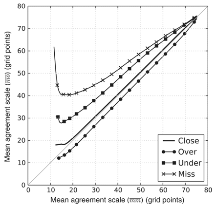
Figure 1Figure reproduced with permission from Dey et al. (2016b) showing results on a binned scatter plot from an idealized experiment indicating the spatial spread–skill relationship between an ensemble forecast and the observation.
To summarize the spread–skill relationship we develop this visualization further by plotting a hexagonal binned 2D histogram plot (an example hexbin plot is presented in Sect. 4.3). The domain is divided into a (pre-determined) number of hexagons. Hexagons minimize the perimeter-to-area ratio and therefore minimize the edge effects. The hexbin histogram plot colour shade represents the number of data points within each bin.
Whilst the hexbin plot is useful for gaining an understanding of the general spread–skill relationship of the ensemble flood map forecast, it does not tell us specifically where in the domain the ensemble spatial predictability is better or worse. Our new spatial spread–skill (SSS) map plots at every grid cell location so that the spread–skill is mapped across the domain and can be linked directly to different sub-catchments and surface features such as tributaries, embankments, bridges and importantly the underlying topography or digital terrain model (DTM), which influence the derivation of the ensemble flood maps. Regions on the SSS map where the ensemble is over-spread are positive with negative areas indicating where the ensemble is under-spread, and zero values show a well-spread ensemble. Note that this does not necessarily mean that the entire ensemble is in agreement with observations at grid level but that the agreement scales between and are equal. (An example SSS map is presented in Sect. 4.3.)
In this section we describe an example flooding event used to demonstrate the application of the spatial spread–skill evaluation approach. We evaluate a 1 d flood inundation 51 ensemble-member forecast from the Flood Foresight system (Sect. 3.2) for the domain area against a satellite SAR-derived flood map (Sect. 3.3).
3.1 Brahmaputra flood, Assam India, August 2017
The origin of the Brahmaputra River (also known as the Yarlung Tsangpo in Tibetan, the Siang and/or Dihang River in Arunachali, Luit in Assamese, and the Jamuna River in Bangladesh) lies in the Himalayan Kailas Range of south-western Tibet, China. Draining an area of 543 000 km2, the Brahmaputra flows for 2000 km across the Tibetan Plateau and a further 1000 km parallel to the Himalayan foothills through the Assam Valley, India, before entering Bangladesh where the Brahmaputra joins the Ganges River (Palash et al., 2020). The Brahmaputra baseflow originates from the upstream glacial snowmelt; however the streamflow rates are dominated by the summer monsoon precipitation. The basin receives up to 95 % of its annual rainfall during the pre-monsoon and monsoon season, which usually runs from April to September and causes annual flooding of the Brahmaputra. The Assam region typically records on average 2300 mm of annual rainfall and up to 5000 mm in the Himalayan foothills (Dhar and Nandargi, 2000, 2003).
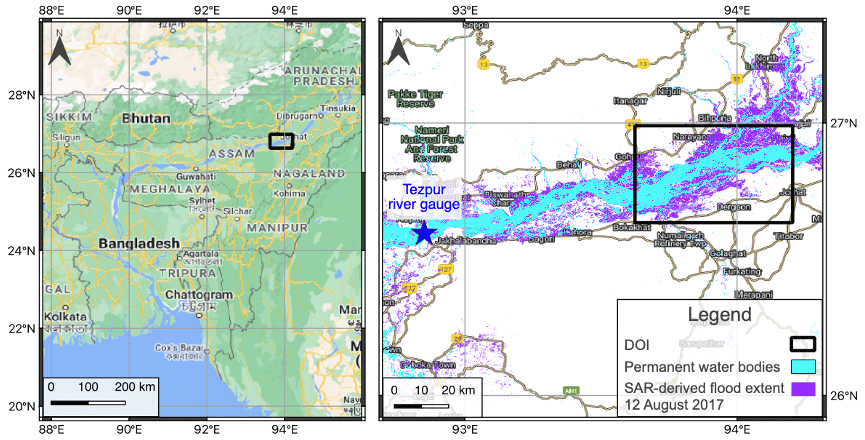
Figure 2Left panel: domain location on the Brahmaputra River in the Assam region of India. Domain size is 57.5 km by 39.3 km. Right panel: Sentinel-1 SAR-derived flood map and permanent water bodies from the JRC Global Surface Water database for the domain of interest (DOI). Base map from © Google Maps.
For this example case we focus on the third wave of flooding that occurred during the monsoon season in August 2017, peaking around 12 August. Figure 2 shows the location of the Brahmaputra and of a chosen domain centred upon some of the worst flooding that occurred. This area includes a confluence zone where the Subansiri River meets the Brahmaputra. The monsoon flooding impacted an estimated 40 million people across India and Bangladesh. Locally in the Assam region, the flooding in August affected over 3.3 million people and approximately 3200 villages, and river embankments were damaged in 11 districts. Over 14 000 people were evacuated to 1 of around 700 relief camps that were also needed to house over 180 000 people relocated (Floodlist, 2017). The local Assam State Disaster Management Authority (ASDMA, 2017) flood early warning system issued a low warning alert (disasters that can be managed at the district level) on 10 August for the district.
In 2017, the south-west monsoon season rainfalls were predicted to be normal by the South Asian Climate Outlook Forum (WMO, 2017). However, the pre-monsoon season began early in the year with heavy thunderstorms affecting the region from March onwards. In the Assam region, June and July were 60 % wetter than the previous 3 years, and during August more locally intense rainfall was recorded compared with historical observations (Palash et al., 2020). In higher-latitude areas, 30 km to the north of the domain at North Lakhimpur, 215.8 mm rainfall was recorded in the 3 d prior to the flood peak (Floodlist, 2017; Hossain et al., 2021). An above-normal flood situation is declared in India where the river water level exceeds the warning level, a severe flood occurs where the water level exceeds the danger level and an extreme flood occurs where the previous highest flood level is exceeded (Central Water Commission, 2023). The peak water level recorded downstream at Tezpur (danger level of 65.23 m) on 14 August was 66.12 m. There are regional variations in maximum water levels reported, with upland regions to the north of the Assam Valley recording water levels that exceed the previous highest flood level, indicating an extreme flood level (Floodlist, 2017).
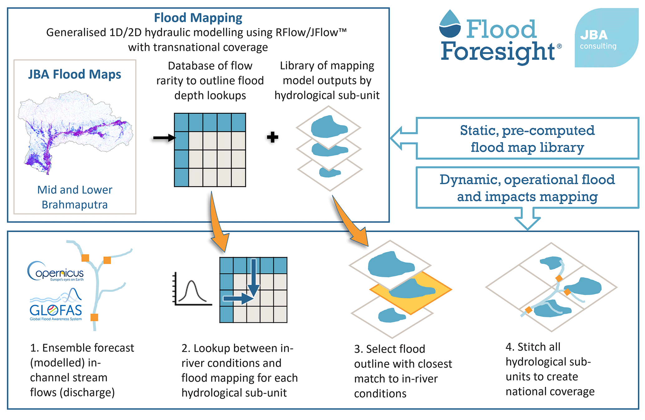
Figure 3The Flood Foresight ensemble forecast flood inundation and impact mapping work flow. Prepared by JBA Consulting.
3.2 Ensemble flood forecasting system
The Flood Foresight system (Fig. 3), developed and operationally run by JBA Consulting, is a fluvial flood inundation mapping system that can be implemented at any river basin around the world. Flood Foresight utilizes a simulation library approach to generate real-time and forecast flood inundation and water depth maps. The simulation library approach saves valuable computing time and allows the application of Flood Foresight in near-continuous real time at national and international scales. A pre-computed library of flood maps for a river basin or country is created using JFlow® (where a DTM is available) (Bradbrook, 2006) and RFlow (where a DTM is unavailable). JFlow uses a raster-based approach with a detailed underlying digital terrain model (DTM) and a diffusion wave approximation of the full 2D hydrodynamic shallow water flow equations. RFlow combines a 1D model based upon normal depth calculations, optimized for use on a digital surface model (DSM; NEXTmap, 2016) with rapid 2D flood spreading (created by spreading normal depth from upstream to downstream) and is calibrated against JFlow. These equations capture the main controls of the flood routing for shallow, topographically driven flow. Six flood maps at 30 m resolution are created for 20-, 50-, 100-, 200-, 500- and 1500-year return period flood events (corresponding to annual exceedance probabilities (AEPs) of 5 %, 2.5 %, 1 %, 0.5 %, 0.2 % and 0.07 %, respectively). Between each adjacent pair of modelled return period maps, five additional intermediate flood maps are created by linear interpolation of both flood depth and extent. An additional five flood maps are also created beneath the lowest return period flood map. This gives, in total, a library of 36 flood maps. Note that these flood maps are undefended, and local, temporary flood defences are not included. Flood Foresight is set up for a region by dividing the river basin into sub-catchments using the HydroBASINS dataset (level 12) (Lehner, 2014). Flood Foresight takes gridded inputs of ensemble forecast streamflow and uses these to select the most appropriate flood map for each sub-catchment. These are mosaicked together, and forecasts of ensemble flood maps are produced daily, out to 10 d ahead.
The global (non-UK and Ireland) configuration of Flood Foresight uses ensemble streamflow forecast data from the Global Flood Awareness System (GloFAS) (Alfieri et al., 2013; GloFAS, 2021). GloFAS was jointly developed by the European Commission and the European Centre for Medium-range Weather Forecasts (ECMWF) and is composed of an integrated hydro-meteorological forecasting chain that couples state-of-the-art weather forecasts with a land surface and hydrological model. With its continental-scale set-up, GloFAS provides downstream countries with forecasts of upstream river conditions up to 1 month ahead, as well as continental and global overviews for large world river basins. Meteorological forecast data are provided by the ECMWF Ensemble (IFS) model, the operational (51-member) ensemble weather forecasting product of the ECMWF. The meteorological forecast data provide inputs to the land surface module, HTESSEL (Hydrological Tiled ECMWF Scheme for Surface Exchange over Land). HTESSEL simulates the land surface response to the meteorological data, based on simulated interactions with soil conditions, idealized vegetation cover and land cover. From these simulations, HTESSEL outputs forecast global surface and sub-surface flows per grid cell. These simulated flows are then used by a simplified version of the hydrological model LISFLOOD, a 1D routing model that simulates the movement of the surface and sub-surface flows. The runoff data produced are routed through a representation of the river network using a double kinematic wave approach, which includes bankfull and over-bankfull routing. The river network used is taken from the HydroSHEDS dataset (Lehner and Grill, 2013).
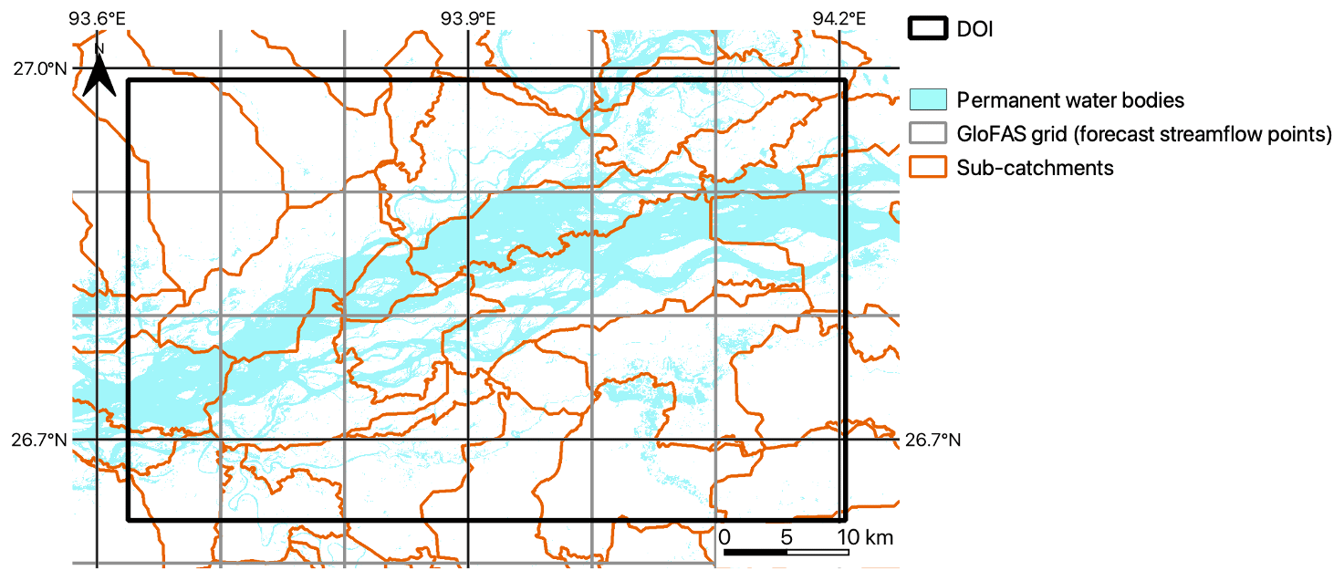
Figure 4GloFAS grid, permanent water bodies and Flood Foresight sub-catchments for the domain of interest (DOI).
GloFAS outputs a gridded (approximately 10 km spatial resolution) ensemble forecast of river streamflow (Fig. 4). Each of the GloFAS grid cells are linked to the sub-catchments in the Flood Foresight system. The simulation library flood maps are selected when the forecast streamflow exceeds a return period (RP) threshold level within each sub-catchment. The RP threshold levels are calculated using ERA5 reanalysis data (Harrigan et al., 2020). Each ensemble-member flood map forecast is created by aggregating the individual sub-catchment maps. In summary, the meteorological IFS 51-member ensemble input to the flood forecasting chain allows atmospheric evolution uncertainties to be represented within the ensemble streamflow forecast and the ensemble of inundation flood maps, thus creating a probabilistic flood map forecast, indicating the likelihood of flooding. Flood Foresight produces daily ensemble flood depth and extent forecasts at 30 m spatial resolution out to 10 d.
3.3 SAR-derived flood map
A Sentinel-1 (S1A) image was acquired in interferometric wide swath mode (swath width of 250 km) around the time of the flood peak at 17:18 (IST) on 12 August 2017. The ESA Grid Processing on Demand (GPOD) HASARD service (service terminated June 2021) was utilized to map the flooding. The flood-mapping algorithm (Chini et al., 2017) uses an automated, statistical, hierarchical split-based approach to distinguish between two classes (background and flood) using a pre-flood and flood image. A pre-flood image (February 2017) from the same satellite sensor and track was used to derive the flood map (Fig. 2). Original SAR images (VV polarization) were pre-processed, which involved precise orbit correction, radiometric calibration, thermal noise removal, terrain correction, speckle reduction and re-projection to the WGS84 coordinate system. The HASARD mapping algorithm removes permanent water bodies that are detected on the pre-flood image, such as the unflooded river water, lakes and reservoirs, by applying a thresholding approach. Flooded areas beneath vegetation, under bridges and near buildings will not be detected using this method. Flood Foresight forecast flood maps include the river channel and exclude surface features such as vegetation and buildings. To smooth the HASARD flood maps and allow a fairer comparison we apply a morphological closing operation (without impacting the location of the flood extent) to flood-fill vegetation and buildings. The wide and braided Brahmaputra River in the Assam region covers a significant area of the selected domain. In order to evaluate the flood prediction accuracy alone, the pre-flood occurrence of surface water using the JRC Global Surface Water database (Pekel et al., 2016) has been removed from the Flood Foresight forecast inundation maps. The observed flood extent derived from satellite-based SAR data at 20 m grid size is re-scaled to match the forecast flood map grid size (30 m) using average aggregation. The closest available (cloud-free) optical image available was a Sentinel-2 image on the 17 August 2017, 5 d after the SAR image acquisition. During this time the flood waters had receded from their peak, which makes this unsuitable for comparison with the SAR-derived flood map. Since no other validation sources are available, for the purposes of this study we have assumed that the SAR-derived observation of flooding represents the true flooding extent. Since October 2021, Sentinel-1 SAR images have been processed by CEMS GFM (GFM, 2021) to derive flooding extent and provide an uncertainty estimate of the grid cell classification. This means uncertainty information in the SAR-derived flood map could be accounted for in future evaluation studies by verification across different levels of observation uncertainty. Additionally, a flood mask, indicating areas where flood detection using SAR data is not currently possible (at the Sentinel-1 spatial resolution), could be used to exclude areas from the evaluation process (note that this was not possible for this case study, since this information was not available in 2017).
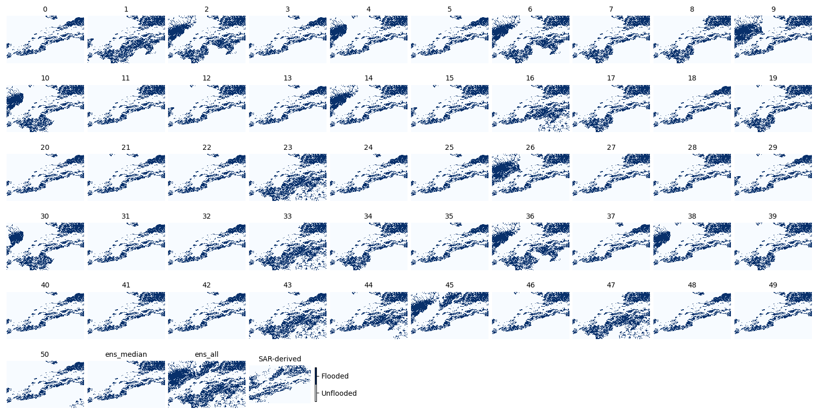
Figure 5Brahmaputra River, Assam region, August 2017. 51 ensemble-member forecast flood maps (labelled 0 to 50), ensmedian and ensall all at 1 d lead time and the Sentinel-1 SAR-derived flood map.
3.4 Forecast data
Flood Foresight was set up for the Brahmaputra basin in India and Bangladesh using the simulation library approach to flood mapping described in Sect. 3.2. Flood maps were pre-computed for the domain of interest (Fig. 2) using a DSM and RFlow. The forecast data for the Brahmaputra flood event contain a 51-member ensemble of flood maps indicating flooding extent, produced at a 1 d lead time. Vertically stacking each individual ensemble-member flood map and adding vertically across every grid cell combines all ensemble members into a single flood map (all flooded grid cells are set to 1) showing where flooding is possible across all members (ensall). A spatial median flood map is created (ensmedian) where 26 members or more predict flooding at a particular grid cell location. Each of the ensemble-member flood maps for the domain is plotted in Fig. 5 along with ensall, ensmedian and the SAR-derived flood map.
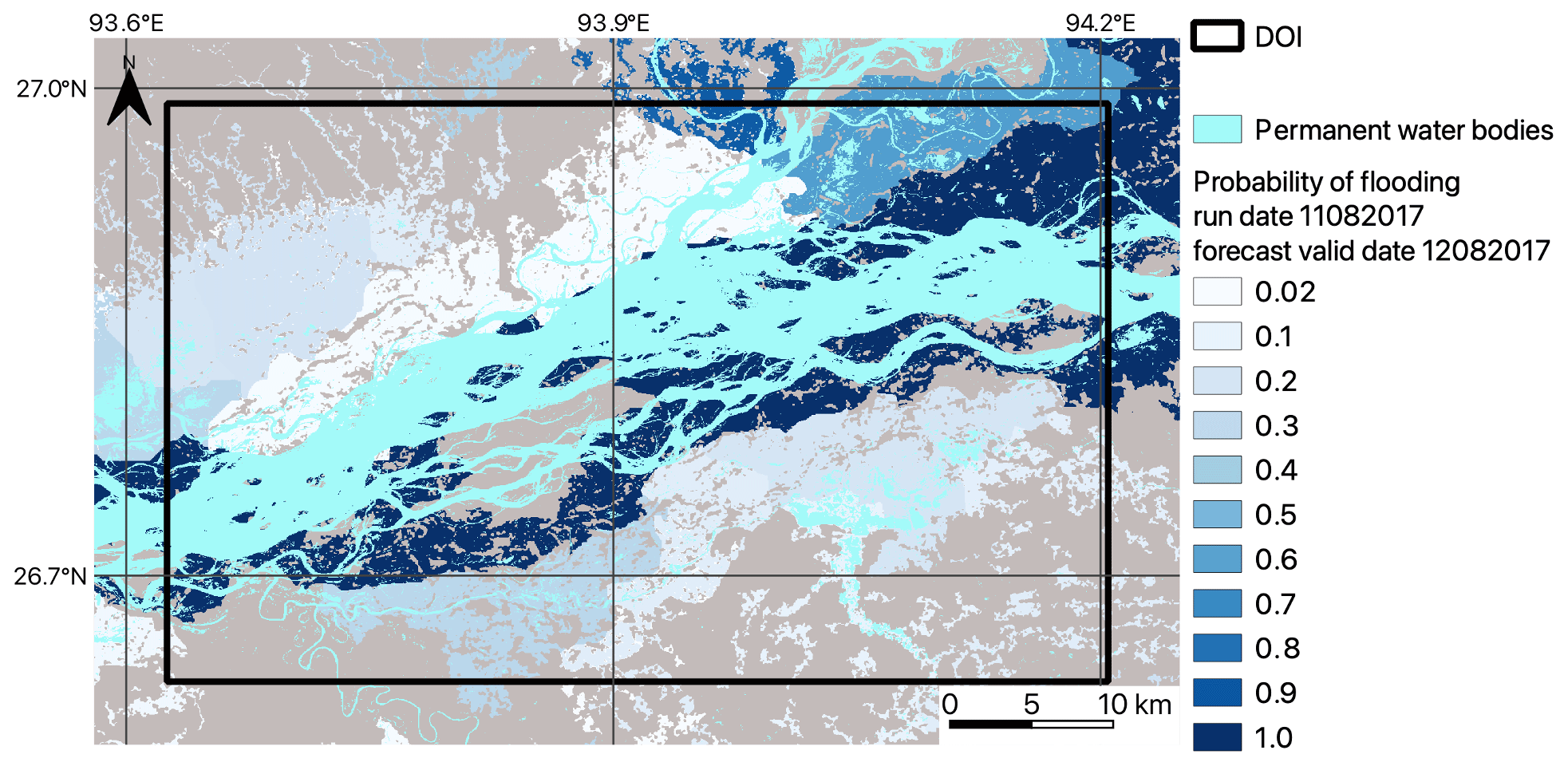
Figure 6Brahmaputra River, Assam region, August 2017. Colour shading from white (low) to dark blue (high) indicates the forecast probability of flooding based on a 1 d lead time, 51 ensemble-member flood map forecast for the Brahmaputra River in the Assam region, August 2017 (note that the map background is grey).
Figure 6 shows the amalgamated probabilistic ensemble forecast indicating the probability of flooding at each grid cell location. This was produced by vertically stacking each ensemble-member flood map and vertically adding the number of flooded cells at each grid cell location across all ensemble members. The total is divided by 51 to calculate the probability. The dark blue colours near the central river channel indicate agreement between all ensemble members and 100 % forecast probability of flooding, and lighter colours to the north of the river indicate a low probability of flooding.
To demonstrate an application of the spatial-scale approach to both ensemble forecast flood map evaluation of forecast skill and the spatial spread–skill relationship, we apply the methods outlined in Sect. 2 to the flooding case described in Sect. 3.1. First, in Sect. 4.1 we verify the full ensemble using a spatial-scale approach to calculate a skilful scale of agreement between each ensemble member and the SAR-derived flood map (Fig. 2) along with the combined ensemble (ensall) and the ensemble spatial median (ensmedian). We evaluate the location-specific spatial skill of the ensemble by calculating categorical-scale maps (Sect. 4.2) for ensall, ensmedian and a best and worst case ensemble member determined by the skilful scale calculated in Sect. 4.1. In Sect. 4.3 we evaluate the spatial predictability of the full ensemble and show this on our new spatial spread–skill (SSS) map, indicating regions where the ensemble is over-spread, under-spread or well-spread.
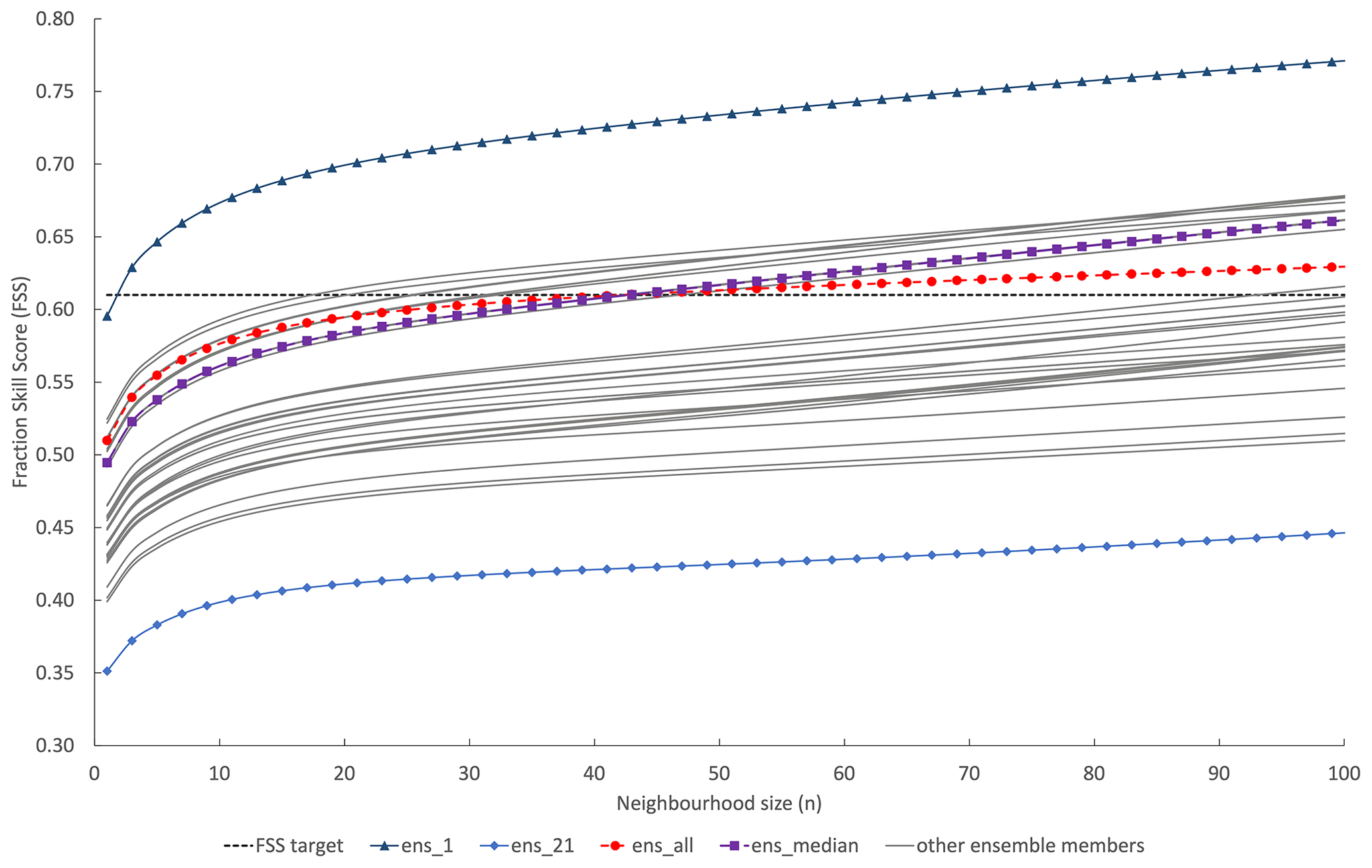
Figure 7The spatial skill of each individual ensemble-member forecast flood extent is evaluated along with the ensmedian (a spatial median where 26 or more members predict flooding at a grid cell location) and ensall (flooded grid cells from all ensemble members are combined). The FSS is calculated at increasing neighbourhood sizes to determine the scale at which the forecast becomes skilful at capturing the observed flood (FSST).
4.1 Ensemble spatial-scale evaluation
Here we investigate how a scale-selective approach can be useful for extracting meaningful information from a flood map ensemble forecast where multiple forecast flood maps represent equally likely flooding scenarios (Fig. 5). A minimum skilful scale (where FSS > FSST) has been calculated for each individual-member flood map, ensall and ensmedian. The results in Fig. 7 show that individual ensemble-member spatial skill varies considerably with FSS at grid level ranging from 0.35 to 0.59. One member ens1, which would usually be disregarded as an outlier due to its low probability, outperformed all other members significantly with a skilful scale achieved at a neighbourhood size of n=3. The combined ensall showed more skill at grid level (n=1) and smaller neighbourhood sizes compared with ensmedian; both however exceeded FSST at n=41 or 600 m. At neighbourhood sizes greater than n=41, ensmedian outperformed ensall. There is a cluster of members showing similar skill to ensmedian and ensall and a second cluster, with more ensemble variation but indicating lower skill than the first cluster. The ensmedian and ensall flood maps outperform the second cluster; however there are individual members with a higher spatial skill score compared to ensmedian and ensall. These results show that all ensemble-member flood maps, including outliers, should be considered individually as possible future flooding scenarios. Spatial variations across individual ensemble members (see Fig. 5 ens1 compared to ensmedian) indicate that it is not meaningful to consider only the ensemble median flood map to represent the information within the full ensemble.
4.2 Ensemble spatial predictability
The scale-selective skill scores calculated for different aspects of the ensemble forecast give a domain-averaged score and skilful scale. To understand location-specific spatial predictability of the ensemble forecast, categorical-scale maps are calculated and presented in Fig. 8. These show how the agreement scale (Sect. 2.2) varies with location for Fig. 8a, ensall; Fig. 8b, ensmedian; Fig. 8c, ens1, the “best”-performing ensemble member; and Fig. 8d, ens21, the “worst”-performing ensemble member. The ensemble summary map ensall (Fig. 8a) captures most of the observed flooding (in grey) with small regions of underprediction (red). However, as you might expect to see by including every potential flooding realization there are significant regions of overprediction (blue) or false alarm. The region of overprediction to the south of the river is less evident in the ensmedian categorical-scale map (Fig. 8b), which performs worse to the north by underpredicting flooding here. This flooding is captured well by ens1 (Fig. 8c) and in particular close to a confluence zone where the Subansiri River joins the Brahmaputra (grid cell location (1100, 250)). This ties in with the high rainfall totals accumulated just to the north of this region associated with localized very heavy rainfall (Floodlist, 2017). A region of underprediction at grid cell location (750, 750) is missed by all members. In future work, a closer inspection of the DTM or surface features included and/or excluded in the hydraulic modelling, such as embankment heights, may indicate how this modelling could be improved. The worst-performing ensemble member ens21 (Fig. 8d) accurately predicts flooding closer to the river channel; however underprediction to the north along with overprediction to the south show where the forecast was inaccurate. Categorical-scale maps enable different ensemble flood map presentations to be evaluated so that the most useful presentation method can be determined for a particular flooding situation.
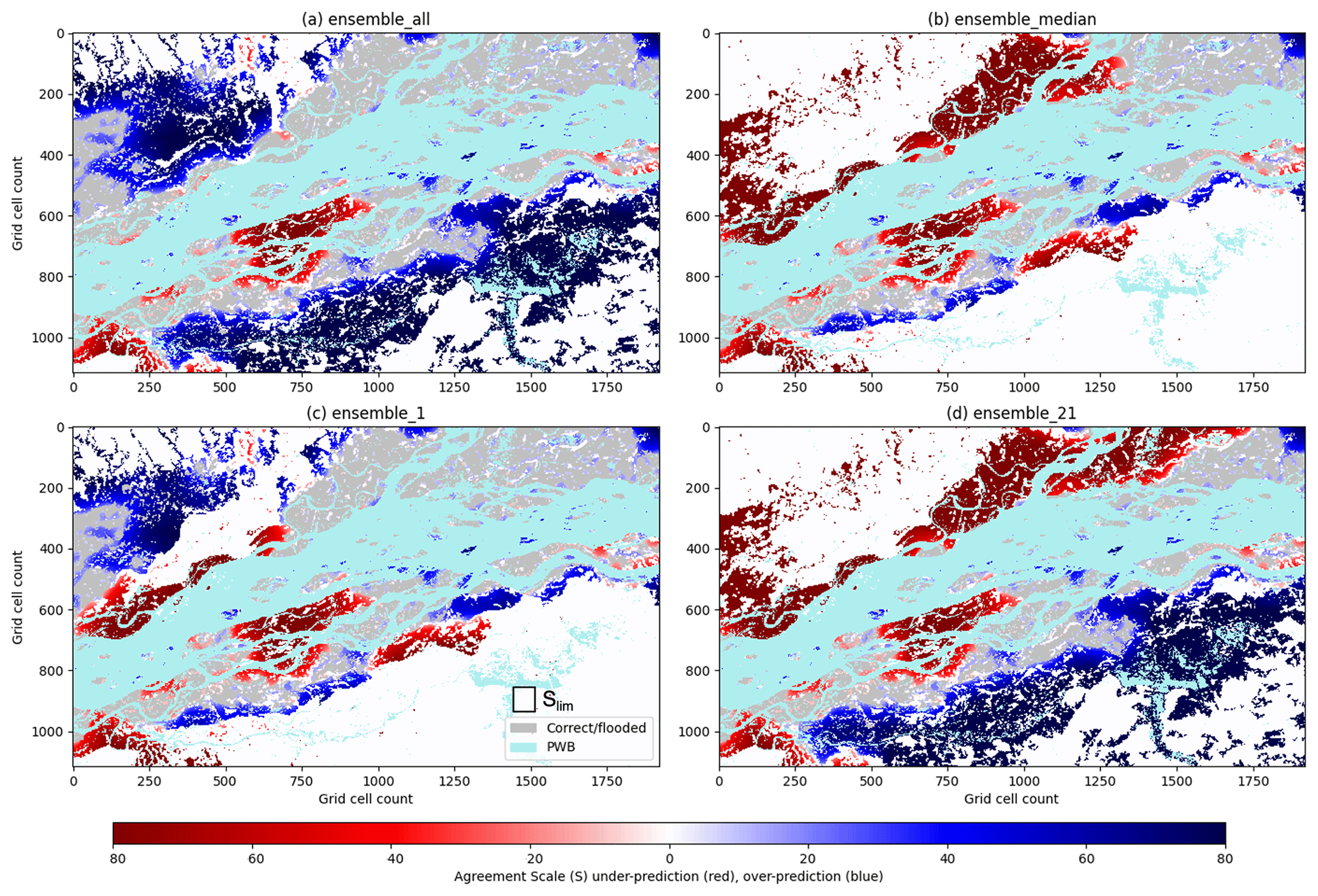
Figure 8Brahmaputra River, Assam region, August 2017. Categorical-scale maps for (a) ensall (flooded grid cells from all ensemble members are combined), (b) ensmedian (a spatial median where 26 or more members predict flooding at a grid cell location), (c) individual ensemble member 1 and (d) individual ensemble member 21. Red areas indicate where the forecast is underpredicted and blue regions represent overprediction. The colour shading indicates the scale of agreement (Eq. 7) between the forecast and the observed flooding, with lighter shading indicating that a smaller agreement scale is required to reach the agreement criterion (Eq. 6). A fixed maximum-scale Slim is drawn to scale (c). For georeferencing, see Fig. 6; each grid cell is 30 m × 30 m.
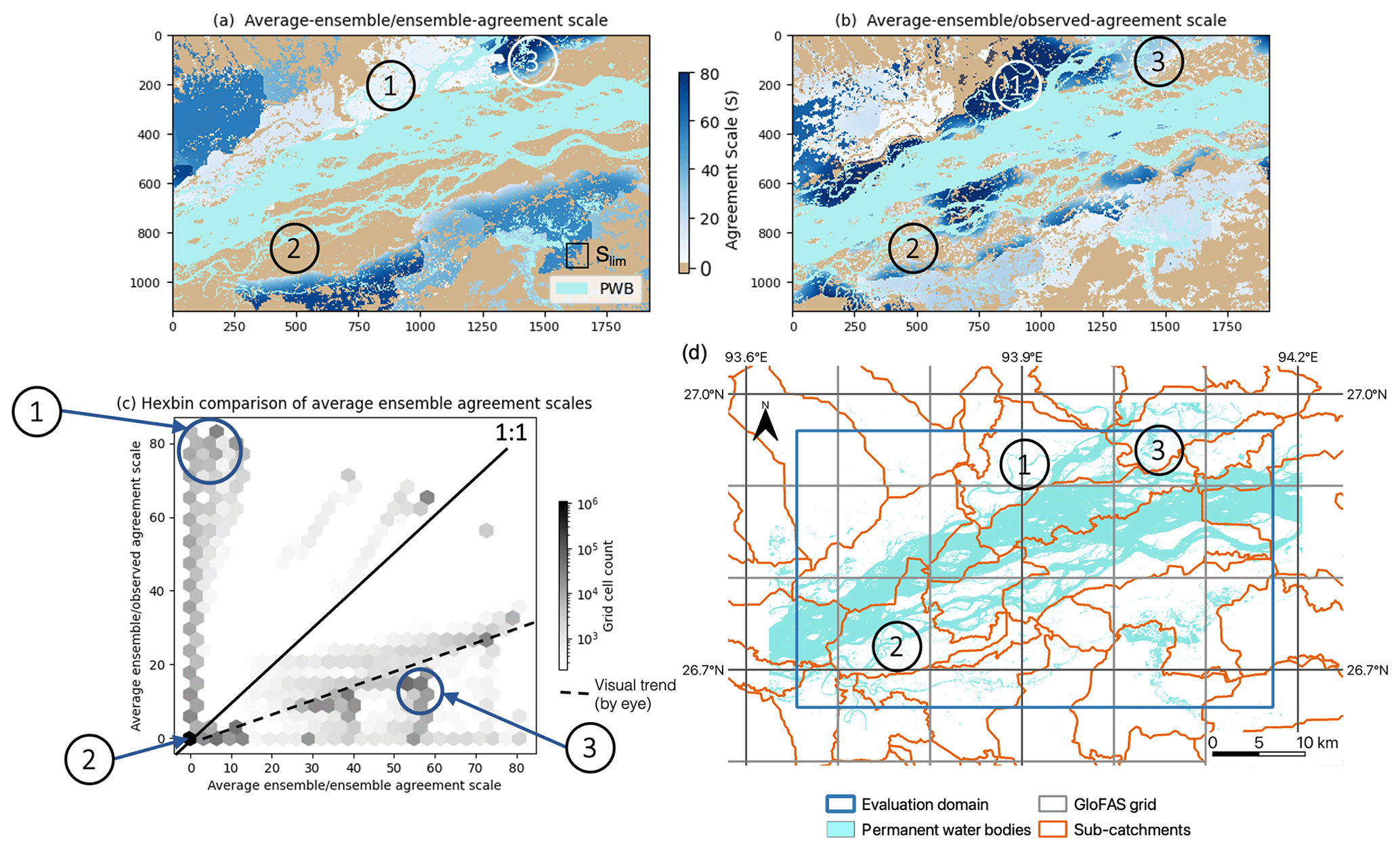
Figure 9Brahmaputra River, Assam region, August 2017. (a) The average agreement-scale map of each unique pair of forecast ensemble flood maps and (b) between each ensemble member compared against the observed SAR-derived flood map. (c) A binned histogram scatter plot compares (a) and (b) to indicate the spatial spread–skill of the forecast ensemble. Panel (d) indicates the corresponding sub-catchment locations. Areas labelled 1, 2 and 3 are discussed in Sect. 4.3. A fixed maximum-scale Slim (Eq. 6) is drawn to scale (a). Note that PWB means permanent water bodies.
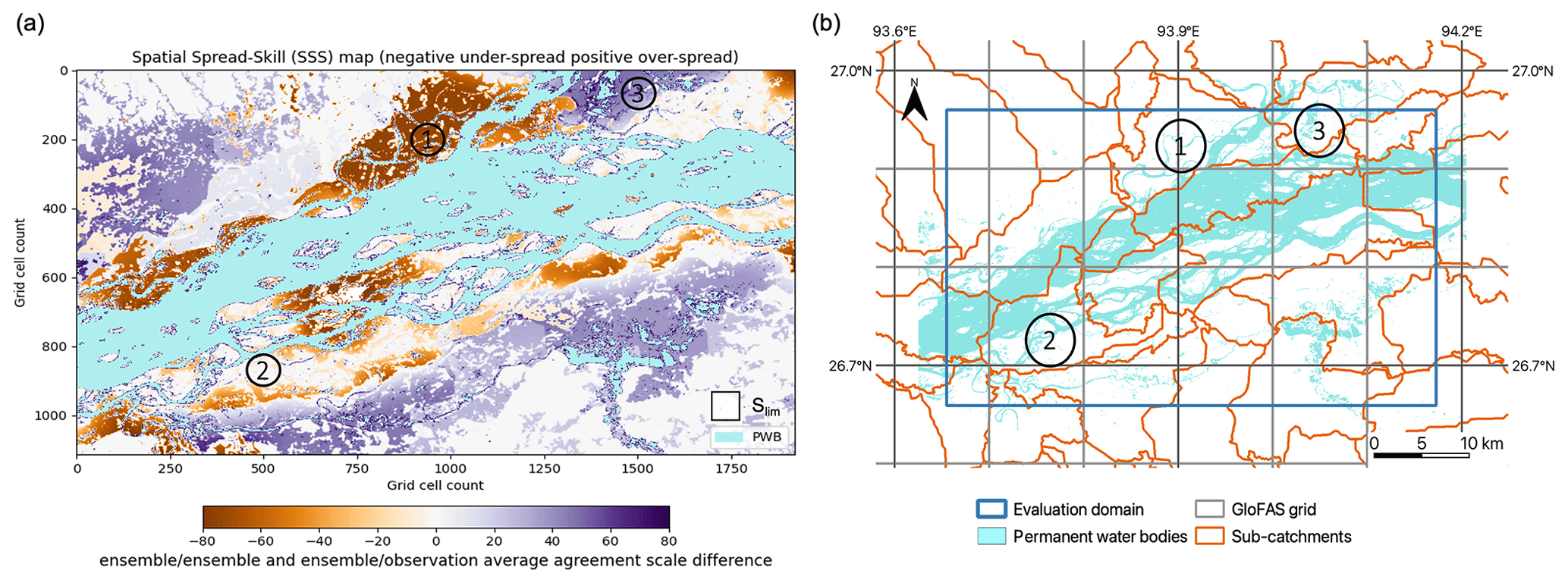
Figure 10Brahmaputra River, Assam region, August 2017. (a) The spatial spread–skill (SSS) map shows the difference between the ensemble–ensemble and the ensemble–observed average agreement scales at each grid cell. Negative values (orange) indicate where the ensemble is under-spread and positive values (purple) indicate where the ensemble is over-spread. White areas indicate where the average agreement scales match and indicate good spatial spread–skill. Panel (d) indicates the corresponding sub-catchment locations. The labelled areas (1, 2 and 3) are discussed in Sect. 4.3. A fixed maximum-scale Slim (Eq. 6) is drawn to scale (a). Note that PWB means permanent water bodies.
4.3 Ensemble spatial spread–skill
To evaluate the location-specific skill of the full ensemble, one option would be to calculate 51 categorical-scale maps from each individual-member flood map (Fig. 5). Although this approach maintains the spatial detail held within each of the ensemble-member flood maps, it does require multiple visual comparisons to be made by the flood forecaster or modeller, which takes time and effort. Making comparisons across the different ensemble-member flood maps in Fig. 5 provides a demonstration of these forecasting difficulties. Further, the categorical-scale maps do not evaluate the ensemble spatial spread. To address this, we develop a spatial spread–skill (SSS) map (derived from Fig. 9, presented in Fig. 10) showing the spread–skill of the full ensemble forecast and keeping the location-specific detail. All ensemble members are included in this analysis which evaluates both the spatial skill and the ensemble spatial spread of the forecast against the remotely observed flooding extent.
Figure 9 shows how the average ensemble–ensemble agreement scale in Fig. 9a calculated at each grid cell (representing ensemble spread) compares with the average ensemble–observed scale in Fig. 9b (representing ensemble skill) along with the hexbin scatter plot in Fig. 9c, which compares Fig. 9a and b to indicate the spatial spread–skill of the forecast. The hexagonal tessellation is used so that the distances along the hexbin diagonal are on the same scale as those along the x and y axis. For a perfect ensemble forecast the average agreement scale between ensemble members should match the agreement scale between the ensemble forecast and observed flood map; i.e. they should align along the 1:1 line. The SSS map plots the difference between the ensemble–ensemble and the ensemble–observed average agreement scales at each grid cell (Fig. 10) and indicates where the spatial spread–skill is over-spread, under-spread, or well-spread. Three numbered areas (Fig. 9a) identify three different ensemble spread–skill relationships. Area 1 shows that the agreement between ensemble members is close but that they disagree with the observed flooding extent. This is displayed in orange shades as an under-spread or missed region on the SSS map in Fig. 10. This is the region close to the confluence area described in Sect. 4.2. Recall that in this region most ensemble members did not predict the flooding that occurred with the exception of one ensemble member (ens1). In area 2 in Fig. 9, both Fig. 9a and Fig. 9b are in agreement at the grid level, which indicates the ensemble is well-spread: these are shown in white in Fig. 10. Apart from the missed and well-spread regions in Fig. 9, the overall visual impression is that the ensemble spread–skill lies below the 1:1 line and is over-spread, indicated by area 3. This corresponds to the purple shading on the SSS map (Fig. 10). Overall Fig. 9 tells us that the spread–skill relationship for this example case study is not uniform across the domain but is in fact location specific. The areas identified (1, 2 and 3) lie within different sub-catchments, which are linked to different GloFAS grid cells, driving the ensemble flood map selection for each sub-catchment. Inferences can be made about the spread–skill of the driving discharge data at sub-catchment level across the domain. Using the spatial spread–skill relationship shown on the ensemble SSS map we can infer how well the ensemble forecasting system encompasses the multiple sources of uncertainty and how meaningful the probabilistic ensemble forecast of flood inundation actually is. An ensemble flood map forecast that is well-spread suggests that the probabilistic forecast is meaningful. The SSS map is a useful evaluation tool for validating flood forecasts in un-gauged or partially gauged rivers. A simulation library approach, like the Flood Foresight maps used here, relies on the accuracy of the return period thresholds set, the (ensemble) forecast streamflow and the accuracy of the flood inundation map for a given streamflow. The forecast evaluation approaches presented here enable these system attributes to be evaluated even where observed streamflow is limited or erroneous. The SSS map summarizes the whole ensemble, which makes it useful for forecasters attempting to convey uncertainty information to decision makers, highlighting regions where there is high or low confidence in the forecast.
Differences between ensemble members in ensemble forecast flood map systems are mostly driven by initial condition perturbations at the top of the hydro-meteorological forecast chain within the numerical weather prediction system. Presently, there is limited understanding or evaluation of how these meteorological uncertainties link to mapped flooding predictability, which involves additional sources of uncertainty. An evaluation of the spatial predictability and the spread–skill relationship of the ensemble flood map forecast provides an improved understanding of the performance of the forecast system. Uncertainties in other parts of the forecast chain are not truly represented by the ensemble flood maps, and evaluating the spatial spread–skill of the flood maps is important for understanding the likelihood of flooding that the ensemble flood maps capture. In this paper, we present a new scale-selective approach to assess the spatial predictability and spread–skill of an ensemble flood map forecast by comparing this against a satellite SAR-derived observation of flooding extent. By calculating a skilful scale at each grid cell for every unique ensemble-member pair we can determine the ensemble spatial spread, and between every ensemble member and the SAR-derived flood map we can determine the ensemble spatial skill. The hexbin scatter plot summarizes the spread–skill relationship so that a trend across the whole domain can be assessed. The difference between these skilful scales can be mapped onto the spatial spread–skill (SSS) map, which shows, for each specific location in the domain, whether the ensemble is over-spread, under-spread or well-spread. The methods are applied to an example flooding event of the Brahmaputra River in the Assam region of India in August 2017.
In operational practice there are multiple options of ensemble flood map presentation type such as presenting the ensemble median or another exceedance probability for delivery to end users and decision makers. An important aspect of developing an inundation flood forecasting system is to determine the most useful way to present a spatial ensemble forecast. Using a scale-selective approach we have evaluated the performance of individual ensemble members, a combined total ensemble and the spatial ensemble median compared to a SAR-derived observation of flooding extent. Other options could be to exclude ensemble-member outliers, to spatially cluster similar ensemble members into groups of flooding extent or to present a most likely, best and worst case ensemble flood map. Whichever presentation method is chosen, this should be fully explored using the spatial spread–skill methods described here to evaluate the ensemble performance of historical flooding events. We found for this example flooding event that one ensemble member significantly outperformed the combined and median flood maps and that potentially in some flood forecasting scenarios this member would have been excluded as an outlier. The categorical-scale maps show that the ensemble spatial median could miss vital flooding information and that all members should be considered potential future flooding scenarios.
Through mapping the spatial spread–skill relationship, which varies with location, links can be made between the spatial variations in spread–skill and the physical characteristics of the flooding event. We found that one ensemble member outperformed all others in a region close to a confluence zone and nearby observed heavy rainfall. The region correlates with an area of under-spread ensemble members, indicating that not enough members were predicting flooding here. Future studies could investigate the physical processes further using the methods presented here. The ensemble flood map spatial spread–skill could be investigated in the context of a particular physical process (such as rainfall intensity and/or location or an improved aspect of the hydrological model such as antecedent soil moisture) and how these uncertainties translate to the probabilistic flood map forecast. An understanding of the spatial predictability is particularly important for un-gauged catchments where the calibration of both forecast streamflow and return period thresholds (used to select the simulation library flood map) is rarely practised routinely. Ideally, in operational practice, these spatial verification approaches including the categorical-scale and SSS maps could be calculated and stored routinely as flooding events coincide with SAR-derived or other remotely observed flood maps to build up a verification catalogue or database. This database could then be used to investigate the spatial spread–skill model performance under different scenarios such as forecast lead time, month or season, or flood type. More locally, the impact of an improved DTM or the inclusion of a digital surface model (DSM) or other surface features in the hydraulic model such as embankments could be considered. Over time, such a database would improve our understanding of the spatial predictability of an ensemble flood map system and how well the uncertainties present are represented by the ensemble forecast.
The functions used to evaluate the ensemble forecast flood maps using a scale-selective approach along with the SAR-derived flood maps are available on the following Zenodo page: https://doi.org/10.5281/zenodo.6603101 (Hooker et al., 2022b). The forecast flood maps from the JBA Flood Foresight system are commercial data used under license for this study.
JB and KS provided the forecast data. HH wrote the algorithms and ran the experiments, with input from SLD, DCM, JB and KS. HH prepared the paper with contributions from all the co-authors.
The contact author has declared that none of the authors has any competing interests.
Publisher's note: Copernicus Publications remains neutral with regard to jurisdictional claims in published maps and institutional affiliations.
This article is part of the special issue “Advances in pluvial and fluvial flood forecasting and assessment and flood risk management”. It is a result of the EGU General Assembly 2022, Vienna, Austria, 23–27 May 2022.
This work was supported in part by the Natural Environment Research Council as part of a SCENARIO-funded PhD project with a CASE award from the JBA Trust (NE/S007261/1). Sarah L. Dance and David C. Mason were funded in part by the UK EPSRC DARE project (EP/P002331/1). Sarah L. Dance also received funding from the NERC National Centre for Earth Observation.
This paper was edited by Kai Schröter and reviewed by Seth Bryant and three anonymous referees.
Alfieri, L., Burek, P., Dutra, E., Krzeminski, B., Muraro, D., Thielen, J., and Pappenberger, F.: GloFAS – global ensemble streamflow forecasting and flood early warning, Hydrol. Earth Syst. Sci., 17, 1161–1175, https://doi.org/10.5194/hess-17-1161-2013, 2013. a
Alfonso, L., Mukolwe, M. M., and Di Baldassarre, G.: Probabilistic Flood Maps to support decision-making: Mapping the Value of Information, Water Resour. Res., 52, 1026–1043, https://doi.org/10.1002/2015WR017378, 2016. a
Anderson, S. R., Csima, G., Moore, R. J., Mittermaier, M., and Cole, S. J.: Towards operational joint river flow and precipitation ensemble verification: considerations and strategies given limited ensemble records, J. Hydrol., 577, 123966, https://doi.org/10.1016/j.jhydrol.2019.123966, 2019. a, b
Arnal, L., Anspoks, L., Manson, S., Neumann, J., Norton, T., Stephens, E., Wolfenden, L., and Cloke, H. L.: “Are we talking just a bit of water out of bank? Or is it Armageddon?” Front line perspectives on transitioning to probabilistic fluvial flood forecasts in England, Geosci. Commun., 3, 203–232, https://doi.org/10.5194/gc-3-203-2020, 2020. a
ASDMA: Assam State Disaster Management Authority Flood Alert, https://asdma.assam.gov.in/information-services/assam-flood-report (last access: 10 November 2021), 2017. a
Ben Bouallègue, Z. and Theis, S. E.: Spatial techniques applied to precipitation ensemble forecasts: From verification results to probabilistic products, Meteorol. Appl., 21, 922–929, https://doi.org/10.1002/met.1435, 2014. a
Beven, K.: Facets of uncertainty: Epistemic uncertainty, non-stationarity, likelihood, hypothesis testing, and communication, Hydrolog. Sci. J., 61, 1652–1665, https://doi.org/10.1080/02626667.2015.1031761, 2016. a
Boelee, L., Lumbroso, D. M., Samuels, P. G., and Cloke, H. L.: Estimation of uncertainty in flood forecasts–A comparison of methods, J. Flood Risk Manage., 12, e12516, https://doi.org/10.1111/jfr3.12516, 2019. a
Bradbrook, K.: JFLOW: A multiscale two-dimensional dynamic flood model, Water Environ. J., 20, 79–86, https://doi.org/10.1111/j.1747-6593.2005.00011.x, 2006. a
Buizza, R.: Potential forecast skill of ensemble prediction and spread and skill distributions of the ECMWF ensemble prediction system, Mon. Weather Rev., 125, 99–119, https://doi.org/10.1175/1520-0493(1997)125<0099:PFSOEP>2.0.CO;2, 1997. a
Central Water Commission: Flood Forecast Dashboard, https://cwc.gov.in/ffm_dashboard (last access: 23 January 2023), 2023. a
Chen, X., Yuan, H., and Xue, M.: Spatial spread-skill relationship in terms of agreement scales for precipitation forecasts in a convection-allowing ensemble, Q. J. Roy. Meteor. Soc., 144, 85–98, https://doi.org/10.1002/qj.3186, 2018. a
Chini, M., Hostache, R., Giustarini, L., and Matgen, P.: A hierarchical split-based approach for parametric thresholding of SAR images: Flood inundation as a test case, IEEE T. Geosci. Remote., 55, 6975–6988, https://doi.org/10.1109/TGRS.2017.2737664, 2017. a
Cloke, H. L. and Pappenberger, F.: Ensemble flood forecasting: A review, J. Hydrol., 375, 613–626, https://doi.org/10.1016/j.jhydrol.2009.06.005, 2009. a
Cooper, E. S., Dance, S. L., Garcia-Pintado, J., Nichols, N. K., and Smith, P. J.: Observation impact, domain length and parameter estimation in data assimilation for flood forecasting, Environ. Model. Softw., 104, 199–214, https://doi.org/10.1016/J.ENVSOFT.2018.03.013, 2018. a
Cooper, E. S., Dance, S. L., García-Pintado, J., Nichols, N. K., and Smith, P. J.: Observation operators for assimilation of satellite observations in fluvial inundation forecasting, Hydrol. Earth Syst. Sci., 23, 2541–2559, https://doi.org/10.5194/hess-23-2541-2019, 2019. a
Copernicus Programme: Copernicus Emergency Management Service, https://emergency.copernicus.eu/ (last access: 14 September 2021), 2021. a
Dasgupta, A., Grimaldi, S., Ramsankaran, R., Pauwels, V. R. N., Walker, J. P., Chini, M., Hostache, R., and Matgen, P.: Flood Mapping Using Synthetic Aperture Radar Sensors From Local to Global Scales, in: Global Flood Hazard, AGU – American Geophysical Union, 55–77, https://doi.org/10.1002/9781119217886.ch4, 2018a. a
Dasgupta, A., Grimaldi, S., Ramsankaran, R. A., Pauwels, V. R., and Walker, J. P.: Towards operational SAR-based flood mapping using neuro-fuzzy texture-based approaches, Remote Sens. Environ., 215, 313–329, https://doi.org/10.1016/j.rse.2018.06.019, 2018b. a
Dasgupta, A., Hostache, R., Ramasankaran, R., Schumann, G. J., Grimaldi, S., Pauwels, V. R. N., and Walker, J. P.: On the impacts of observation location, timing and frequency on flood extent assimilation performance, Water Resour. Res., https://doi.org/10.1029/2020wr028238, 2021a. a
Dasgupta, A., Hostache, R., Ramsankaran, R. A., Schumann, G. J., Grimaldi, S., Pauwels, V. R., and Walker, J. P.: A Mutual Information-Based Likelihood Function for Particle Filter Flood Extent Assimilation, Water Resour. Res., 57, 1–28, https://doi.org/10.1029/2020WR027859, 2021b. a
Dey, S. R., Leoncini, G., Roberts, N. M., Plant, R. S., and Migliorini, S.: A spatial view of ensemble spread in convection permitting ensembles, Mon. Weather Rev., https://doi.org/10.1175/MWR-D-14-00172.1, 2014. a, b
Dey, S. R., Plant, R. S., Roberts, N. M., and Migliorini, S.: Assessing spatial precipitation uncertainties in a convective-scale ensemble, Q. J. Roy. Meteor. Soc., https://doi.org/10.1002/qj.2893, 2016a. a
Dey, S. R., Roberts, N. M., Plant, R. S., and Migliorini, S.: A new method for the characterization and verification of local spatial predictability for convective-scale ensembles, Q. J. Roy. Meteor. Soc., https://doi.org/10.1002/qj.2792, 2016b. a, b, c, d, e
Dhar, O. N. and Nandargi, S.: A study of floods in the Brahmaputra basin in India, Int. J. Climatol., 20, 771–781, https://doi.org/10.1002/1097-0088(20000615)20:7<771::AID-JOC518>3.0.CO;2-Z, 2000. a
Dhar, O. N. and Nandargi, S.: Hydrometeorological Aspects of Floods in India, Springer Netherlands, Dordrecht, 1–33, https://doi.org/10.1007/978-94-017-0137-2_1, 2003. a
Di Mauro, C., Hostache, R., Matgen, P., Pelich, R., Chini, M., van Leeuwen, P. J., Nichols, N. K., and Blöschl, G.: Assimilation of probabilistic flood maps from SAR data into a coupled hydrologic–hydraulic forecasting model: a proof of concept, Hydrol. Earth Syst. Sci., 25, 4081–4097, https://doi.org/10.5194/hess-25-4081-2021, 2021. a
Emerton, R. E., Stephens, E. M., Pappenberger, F., Pagano, T. C., Weerts, A. H., Wood, A. W., Salamon, P., Brown, J. D., Hjerdt, N., Donnelly, C., Baugh, C. A., and Cloke, H. L.: Continental and global scale flood forecasting systems, WIREs Water, 3, 391–418, https://doi.org/10.1002/wat2.1137, 2016. a
ESA: ICEYE commercial satellites join the EU Copernicus programme, https://www.esa.int/Applications/Observing_the_Earth/Copernicus/ICEYE_commercial_satellites_join_the_EU_Copernicus_programme (last access: 28 October 2021), 2021. a
EU Science Hub: The Joint Research Centre launches a revolutionary tool for monitoring ongoing floods worldwide as part of the Copernicus Emergency Management Service, https://ec.europa.eu/jrc/en/news/jrc-launches-revolutionary-tool-for-monitoring-floods-worldwide (last access: 28 October 2021), 2021. a
Floodlist: India – Third Wave of Flooding Hits Assam, 2 Million Affected, http://floodlist.com/asia/india-assam-floods-august-2017 (last access: 10 November 2021), 2017. a, b, c, d
Galmiche, N., Hauser, H., Spengler, T., Spensberger, C., Brun, M., and Blaser, N.: Revealing Multimodality in Ensemble Weather Prediction, in: Machine Learning Methods in Visualisation for Big Data, edited by: Archambault, D., Nabney, I., and Peltonen, J., The Eurographics Association, https://doi.org/10.2312/mlvis.20211073, 2021. a
García-Pintado, J., Mason, D. C., Dance, S. L., Cloke, H. L., Neal, J. C., Freer, J., and Bates, P. D.: Satellite-supported flood forecasting in river networks: A real case study, J. Hydrol., 523, 706–724, https://doi.org/10.1016/J.JHYDROL.2015.01.084, 2015. a
GFM: GloFAS global flood monitoring (GFM), https://www.globalfloods.eu/technical-information/glofas-gfm/ (last access: 28 October 2021), 2021. a, b
GloFAS: GloFAS Methods, https://www.globalfloods.eu/general-information/glofas-methods/ (last access: 15 November 2021), 2021. a
Grimaldi, S., Li, Y., Pauwels, V. R., and Walker, J. P.: Remote Sensing-Derived Water Extent and Level to Constrain Hydraulic Flood Forecasting Models: Opportunities and Challenges, Surv. Geophys., 37, 977–1034, https://doi.org/10.1007/s10712-016-9378-y, 2016. a
Harrigan, S., Zsoter, E., Alfieri, L., Prudhomme, C., Salamon, P., Wetterhall, F., Barnard, C., Cloke, H., and Pappenberger, F.: GloFAS-ERA5 operational global river discharge reanalysis 1979–present, Earth Syst. Sci. Data, 12, 2043–2060, https://doi.org/10.5194/essd-12-2043-2020, 2020. a
Hooker, H., Dance, S. L., Mason, D. C., Bevington, J., and Shelton, K.: Spatial scale evaluation of forecast flood inundation maps, J. Hydrol., 612, 128170, https://doi.org/10.1016/j.jhydrol.2022.128170, 2022a. a, b, c, d, e
Hooker, H., Dance, S. L., Mason, D. C., Bevington, J., and Shelton, K.: Ensemble flood map spatial verification [Data set], Zenodo [data set], https://doi.org/10.5281/zenodo.6603101, 2022b. a
Hopson, T. M.: Assessing the ensemble spread-error relationship, Mon. Weather Rev., 142, 1125–1142, https://doi.org/10.1175/MWR-D-12-00111.1, 2014. a
Horritt, M. S., Mason, D. C., and Luckman, A. J.: Flood boundary delineation from synthetic aperture radar imagery using a statistical active contour model, Int. J. Remote Sens., 22, 2489–2507, https://doi.org/10.1080/01431160116902, 2001. a
Hossain, S., Cloke, H. L., Ficchì, A., Turner, A. G., and Stephens, E. M.: Hydrometeorological drivers of flood characteristics in the Brahmaputra river basin in Bangladesh, Hydrol. Earth Syst. Sci. Discuss. [preprint], https://doi.org/10.5194/hess-2021-97, 2021. a
Hostache, R.: A first evaluation of the future CEMS systematic global flood monitoring product, https://events.ecmwf.int/event/222/contributions/2274/attachments/1280/2347/Hydrological-WS-Hostache.pdf (last access: 4 August 2021), 2021. a
Konapala, G., Kumar, S. V., and Khalique Ahmad, S.: Exploring Sentinel-1 and Sentinel-2 diversity for flood inundation mapping using deep learning, ISPRS J. Photogramm., 180, 163–173, https://doi.org/10.1016/J.ISPRSJPRS.2021.08.016, 2021. a
Lehner, B.: HydroBASINS Global watershed boundaries and sub-basin delineations derived from HydroSHEDS data at 15 second resolution, https://www.hydrosheds.org/images/inpages/HydroBASINS_TechDoc_v1c.pdf (last access: 5 November 2022), 2014. a
Lehner, B. and Grill, G.: Global river hydrography and network routing: baseline data and new approaches to study the world's large river systems, Hydrol. Process., 27, 2171–2186, https://doi.org/10.1002/hyp.9740, 2013. a
Leutbecher, M. and Palmer, T. N.: Ensemble forecasting, J. Comput. Phys., 227, 3515–3539, https://doi.org/10.1016/J.JCP.2007.02.014, 2008. a
Lorenz, E. N.: The predictability of a flow which possesses many scales of motion, Tellus, 21, 289–307, https://doi.org/10.3402/tellusa.v21i3.10086, 1969. a
Mason, D. C., Schumann, G. J., Neal, J. C., Garcia-Pintado, J., and Bates, P. D.: Automatic near real-time selection of flood water levels from high resolution Synthetic Aperture Radar images for assimilation into hydraulic models: A case study, Remote Sens. Environ., 124, 705–716, https://doi.org/10.1016/j.rse.2012.06.017, 2012. a
Mason, D. C., Dance, S. L., Vetra-Carvalho, S., and Cloke, H. L.: Robust algorithm for detecting floodwater in urban areas using synthetic aperture radar images, J. Appl. Remote Sens., 12, 1, https://doi.org/10.1117/1.jrs.12.045011, 2018. a
Mason, D. C., Dance, S. L., and Cloke, H. L.: Floodwater detection in urban areas using Sentinel-1 and WorldDEM data, J. Appl. Remote Sens., 15, 1–22, https://doi.org/10.1117/1.jrs.15.032003, 2021a. a
Mason, D. C., Bevington, J., Dance, S. L., Revilla-Romero, B., Smith, R., Vetra-Carvalho, S., and Cloke, H. L.: Improving urban flood mapping by merging synthetic aperture radar-derived flood footprints with flood hazard maps, Water (Switzerland), 13, 1577, https://doi.org/10.3390/w13111577, 2021b. a
Matthews, G., Barnard, C., Cloke, H., Dance, S. L., Jurlina, T., Mazzetti, C., and Prudhomme, C.: Evaluating the impact of post-processing medium-range ensemble streamflow forecasts from the European Flood Awareness System, Hydrol. Earth Syst. Sci., 26, 2939–2968, https://doi.org/10.5194/hess-26-2939-2022, 2022. a
NEXTmap: NEXTMap World30 DSM, https://www.intermap.com/nextmap (last access: 24 January 2023), 2016. a
Palash, W., Akanda, A. S., and Islam, S.: The record 2017 flood in South Asia: State of prediction and performance of a data-driven requisitely simple forecast model, J. Hydrol., 589, 125190, https://doi.org/10.1016/j.jhydrol.2020.125190, 2020. a, b
Pappenberger, F., Beven, K. J., Hunter, N. M., Bates, P. D., Gouweleeuw, B. T., Thielen, J., and de Roo, A. P. J.: Cascading model uncertainty from medium range weather forecasts (10 days) through a rainfall-runoff model to flood inundation predictions within the European Flood Forecasting System (EFFS), Hydrol. Earth Syst. Sci., 9, 381–393, https://doi.org/10.5194/hess-9-381-2005, 2005. a
Pekel, J. F., Cottam, A., Gorelick, N., and Belward, A. S.: High-resolution mapping of global surface water and its long-term changes, Nature, 540, 418–422, https://doi.org/10.1038/nature20584, 2016. a
Renner, M., Werner, M. G., Rademacher, S., and Sprokkereef, E.: Verification of ensemble flow forecasts for the River Rhine, J. Hydrol., 376, 463–475, https://doi.org/10.1016/j.jhydrol.2009.07.059, 2009. a
Roberts, N. M. and Lean, H. W.: Scale-selective verification of rainfall accumulations from high-resolution forecasts of convective events, Mon. Weather Rev., 136, 78–97, https://doi.org/10.1175/2007MWR2123.1, 2008. a, b
Savage, J. T. S., Bates, P., Freer, J., Neal, J., and Aronica, G.: When does spatial resolution become spurious in probabilistic flood inundation predictions?, Hydrol. Process., 30, 2014–2032, https://doi.org/10.1002/hyp.10749, 2016. a
Skok, G. and Roberts, N.: Estimating the displacement in precipitation forecasts using the Fractions Skill Score, Q. J. Roy. Meteor. Soc., 144, 414–425, https://doi.org/10.1002/qj.3212, 2018. a, b
Speight, L. and Krupska, K.: Understanding the impact of climate change on inland flood risk in the UK, Weather, 76, 330–331, https://doi.org/10.1002/wea.4079, 2021. a
Tavus, B., Kocaman, S., Nefeslioglu, H. A., and Gokceoglu, C.: A fusion approach for flood mapping using sentinel-1 and sentinel-2 datasets, Int. Arch. Photogramm., 43, 641–648, https://doi.org/10.5194/isprs-archives-XLIII-B3-2020-641-2020, 2020. a
WMO: South Asian Climate Outlook Forum held in Bhutan, https://public.wmo.int/en/media/news/normal-rainfall-likely-much-of-south-asia-2017-southwest (last access: 23 January 2023), 2017. a
Wu, W., Emerton, R., Duan, Q., Wood, A. W., Wetterhall, F., and Robertson, D. E.: Ensemble flood forecasting: Current status and future opportunities, WIREs Water, 7, 1–32, https://doi.org/10.1002/wat2.1432, 2020. a
Zappa, M., Jaun, S., Germann, U., Walser, A., and Fundel, F.: Superposition of three sources of uncertainties in operational flood forecasting chains, Atmos. Res., 100, 246–262, https://doi.org/10.1016/J.ATMOSRES.2010.12.005, 2011. a
- Abstract
- Introduction
- Ensemble flood map spatial predictability evaluation methods
- Ensemble forecasting flood event case study
- Results and discussion
- Conclusions
- Code and data availability
- Author contributions
- Competing interests
- Disclaimer
- Special issue statement
- Financial support
- Review statement
- References