Apparent contradiction in the projected climatic water balance for Austria: wetter conditions on average versus higher probability of meteorological droughts

In this paper future changes of surface water availability in Austria are investigated. We use an ensemble of downscaled and bias-corrected regional climate model simulations of the EURO-CORDEX initiative under moderate mitigation (RCP4.5) and Paris Agreement (RCP2.6) emission scenarios. The climatic water balance and its components (rainfall, snow melt, glacier melt and atmospheric evaporative demand) are used as indicators of surface water availability, and we focus on different altitudinal classes (lowland, mountainous and high alpine) to depict a variety of processes in complex terrain. Apart from analysing the mean changes of these components, we also pursue a hazard risk approach by estimating future changes in return periods of meteorological drought events of a given magnitude as observed in the reference period. The results show, in general, wetter conditions over the course of the 21st century over Austria on an annual basis compared to the reference period 1981–2010 (e.g. RCP4.5 +107 mm, RCP2.6 +63 mm for the period 2071–2100). Considering seasonal differences, winter and spring are getting wetter due to an increase in precipitation and a higher fraction of rainfall as a consequence of rising temperatures. In summer only little changes in the mean of the climatic water balance conditions are visible across the model ensemble (e.g. RCP4.5 ±0 mm, RCP2.6 −2 mm for the period 2071–2100). On the contrary, by analysing changes in return periods of drought events, an increasing risk of moderate and extreme drought events during summer is apparent, a signal emerging within the climate system along with increasing warming.

1 Introduction

Drought and water scarcity are among the most devastating natural hazards causing damage on various natural and human systems. Average annual economic losses from drought alone are estimated to EUR 9 billion in the European Union (European Commission, 2020). Europe was struck several times in recent years by severe summer droughts, causing enormous economic damage, for example, the drought of 2015 (Laaha et al., 2017; Van Lanen et al., 2016; Ionita et al., 2017) and of 2018 (Buras et al., 2020; Boergens et al., 2020; Bakke et al., 2020), which hit Austria in particular. Future climate change will further alter hydroclimatological conditions in various ways through, for example, shifts in rainfall distribution through intensification of the hydrological cycle (Allan et al., 2020; Vargas Godoy and Markonis, 2022), shifts in seasonality of certain variables (e.g. snow, Mudryk et al., 2020), and large-scale changes in the atmospheric circulation and moisture transport (Fabiano et al., 2021). It is therefore vital to assess possible future changes of multiple input, output and storage terms at the land surface in order to unravel critical processes and thresholds in both space and time which may impact surface water availability.

Austria, with its mountainous topography, is in general considered a water-rich country with freshwater resources by far exceeding the demand (Haas and Birk, 2019; Stelzl et al., 2021). Recent drought years, however, have raised concerns about changing water availability. Precipitation trends on the very long term back to the 19th century show no significant trend, and changes are mostly subject to multidecadal variability (Brunetti et al., 2009; Haslinger et al., 2021). During the past decades, precipitation has slightly increased, though this signal did not appear in the runoff signatures, since it was balanced by increasing atmospheric evaporative demand (Duethmann and Blöschl, 2018). Precipitation in the form of snow plays an important role for surface water availability in mountainous areas. In Austria and the Alpine region in general a significant decline in snow depth is observed (Matiu et al., 2021; Olefs et al., 2020; Schöner et al., 2018) with possible impacts on consequent summer low flows (Jenicek et al., 2016). Considering drought conditions in particular, meteorological droughts show no trends over the past 200 years (Haslinger et al., 2019b; Haslinger and Blöschl, 2017). On the contrary, hydrological droughts exhibit negative trends over the past 40 years, but only over some lowland areas in the north and southeast of Austria (Laaha et al., 2016; Blöschl et al., 2018).

Climate change already alters some aspects of water availability in Austria, mainly due to decreasing snow cover and increasing atmospheric evaporative demand. Climate projections show an increase in precipitation over Austria which is stronger in winter and spring than in summer (Blöschl et al., 2018). Increasing temperatures also act on the future snow cover with specific impacts on drought development and predictability (Livneh and Badger, 2020; Musselman et al., 2021). For Austria in particular, Olefs et al. (2021) highlighted the sensitivity of snow cover to temperature especially below 1500 m a.s.l. Future scenarios for meteorological drought conditions show increasing drought risk particularly during summer under Intergovernmental Panel on Climate Change (IPCC) CMIP3 scenarios (Haslinger et al., 2016; Laaha et al., 2016), which is mainly driven by precipitation decrease and atmospheric evaporative demand increase (see also Gali Reniu, 2017). For river discharge, IPCC CMIP3 projections point towards decreasing summer low flows in lowland areas and increasing winter low flows in the alpine areas of Austria (Laaha et al., 2016; Parajka et al., 2016). Although the body of existing literature points towards changing water availability in Austria, a comprehensive synopsis of all relevant processes altering surface water availability has not been accomplished yet or just for small spatial entities (Hanus et al., 2021). Here we aim to fill this research gap by addressing the following research questions using the Austrian reference climate scenario dataset based on EURO-CORDEX CMIP5 regional climate simulations:

• i.

  How will future surface climatic water balance change under different emission scenarios and different elevations?

• ii.

  How do the individual components of the surface water balance change during the course of the year?

• iii.

  How will the probability of extreme drought conditions change under future climate?

2 Data

In this study we use gridded observations and modelled data. All datasets are on a congruent 1 km grid and fully cover the Austrian domain; see Fig. 1a for the domain boundaries as indicated by coloured topography shading. Considering climate scenarios we use the Austrian national reference scenario dataset OEKS15 (Chimani et al., 2016), which consists of a selected ensemble of regional climate model (RCM) simulations driven by CMIP5 global climate models from the EURO-CORDEX EUR-11 database. The selection of the models is based on quantitative criteria as described in Chimani et al. (2020). Three different emission scenarios are available within OEKS15; here we use RCP4.5 and RCP2.6. With this choice we intend to depict, on the one hand, a likely outcome of emission pathways during the 21st century, where RCP4.5 draws a modest climate change mitigation future and a likely outcome and, on the other hand, a more favourable outcome by meeting the Paris Agreement within the scenario pathway of RCP2.6. The broadly used RCP8.5 scenario is intentionally not included here, since its emission pathway is highly unlikely from today's emissions trajectories, as well as current and pledged policies, and is often misleadingly used as a business-as-usual scenario (Hausfather and Peters, 2020; Pielke and Ritchie, 2021). From today's perspective an emission path following RCP4.5 is, at least until 2030, the most likely one given current estimates (UNFCCC, 2022).

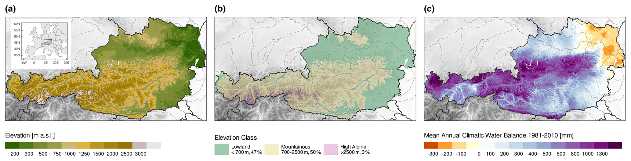
Figure 1 (a) Topography of Austria, with the inset indicating the location in the European domain; (b) altitudinal classification; and (c) long-term mean (1981–2010) annual climatic water balance.

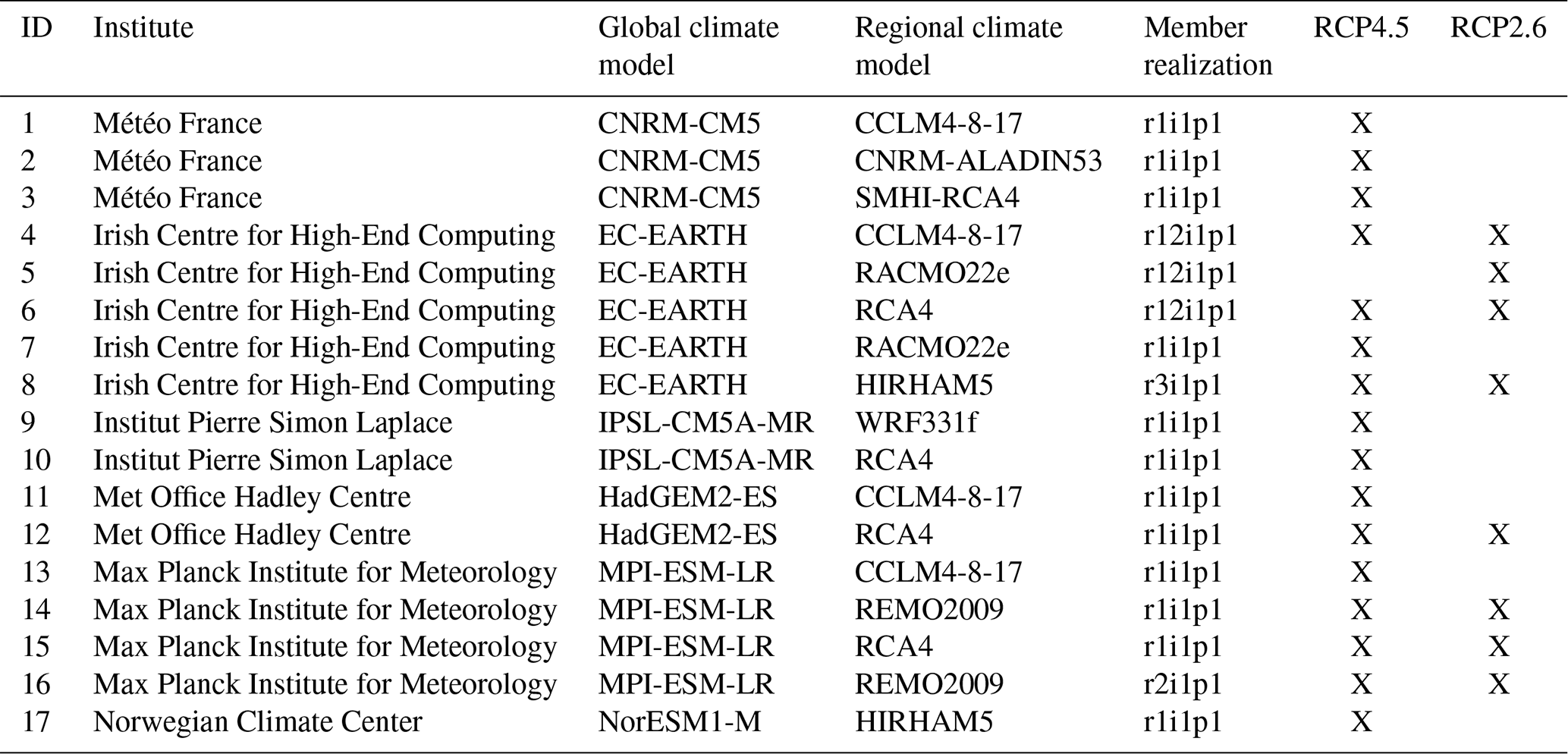
In total 16 model runs are available for RCP4.5 and 8 for RCP2.6; a summary is given in Table 1 indicating the driving global climate model, the RCM and member realization. The EURO-CORDEX simulations are downscaled and bias-corrected using scaled distribution mapping (Switanek et al., 2017), which is an optimized quantile mapping approach (Themeßl et al., 2011) preserving the initial climate change signal of the RCM simulation. As reference datasets for the bias correction, gridded observations of daily maximum and minimum temperatures of SPARTACUS (Spatiotemporal Reanalysis Dataset for Climate in Austria; Hiebl and Frei, 2016) are used as well as GPARD1 (Gridded Precipitation for Austria at Daily 1 km Resolution, Hofstätter et al., 2015) for daily precipitation sums. Both reference datasets consider orographic effects on temperature (e.g. cold air pool formation, foehn effects) and on precipitation (orographic precipitation), which is rather important for interpolating climatic variables in complex terrain of the Austrian domain. The basic datasets for OEKS15 (EURO-CORDEX) were thoroughly evaluated in Kotlarski et al. (2014), and OEKS15 was evaluated with a comprehensive guide line given on the usage in Chimani et al. (2020).

Table 1 RCM simulations used in the present study.

To account for different processes considering changes in water availability along elevation, we stratified the Austrian domain in three different classes of elevation (Fig. 1b). The first denotes the lowland areas below 700 m a.s.l. (47 % of the entire domain), which are mostly comprised of agricultural land and also encompass the major settlement areas and large urban areas. The second elevation class defines mountainous areas between 700 and 2500 m a.s.l. (50 % of the entire domain). These are mostly covered by forests and alpine pastures. The third elevation class denotes high-alpine areas above 2500 m a.s.l. with some alpine pastures and mostly unvegetated terrain and glaciers at the highest altitudes (3 % of the entire domain).

3 Methods

3.1 The climatic water balance

In this paper we use the climatic water balance (CWB) as the basic metric for assessing surface water availability and drought conditions. In principal, the CWB is the difference between precipitation and atmospheric evaporative demand (AED) and is therefore able to depict both atmospheric supply and demand. It is often used to derive the standardized precipitation evapotranspiration index (SPEI; Vicente-Serrano et al., 2010) by fitting a probability distribution function to the CWB and afterwards transforming it into a unit normal distribution. This enables a rather intuitive assessment of the moisture conditions (negative/positive values dryer/wetter than normal) and has made the SPEI a broadly applied index for drought monitoring and forecasting as well as for research purposes (e.g. Haslinger et al., 2014, 2016). Here we stick to the basic CWB to be able to give absolute values of change rather than changing index values, which may be difficult to interpret. The annual mean CWB for the 1981–2010 period is displayed in Fig. 1c. It shows a rather diverse spatial pattern, with positive values in the mountainous western parts of Austria in contrast to distinct negative values in the flat, low-elevation part in the northeast of the country. In general this pattern is mainly driven by spatial patterns of precipitation with the largest precipitation amounts occurring in the so-called Northern Stau regions and the decrease of AED along higher elevations.

For analysing the impacts of future climate change on CWB evolution, we extended this concept by considering the effects of snow accumulation and ablation as well as phase conditions of precipitation (liquid versus solid). This enables the assessment of the changing snow cover conditions along projected temperature increases and potential shifts of water availability during the course of the year and across different elevation zones. Hence for this analysis, CWB is given by the following equation:

$$\begin{array}{}\text{(1)}& \mathrm{CWB}=(R+M)-\mathrm{AED},\end{array}$$

where R stands for liquid precipitation or rainfall, M for snow melt and AED for atmospheric evaporative demand. For the special case of the high-alpine area (cf. Fig. 1b), we also consider glacier melt as an individual positive term in the climatic water balance equation.

3.2 Atmospheric evaporative demand

Atmospheric evaporative demand (AED), or reference evapotranspiration, refers to the maximum moisture flux to the atmosphere from a standardized land surface (grass) under continuous moisture supply and given meteorological conditions (Lhomme, 1997). It is therefore independent from soil properties; hence it is widely used to assess crop water requirements, for example. In this study we use AED estimates following the approach of Haslinger and Bartsch (2016). The authors used the method of Hargreaves (Hargreaves and Allen, 2003; Hargreaves and Samani, 1985), which requires daily maximum and minimum air temperature and latitude as input data. The authors re-calibrated the original Hargreaves parameter against the FAO Penman–Monteith (Allen and Food and Agriculture Organization of the United Nations, 1998) estimates on several stations across Austria. This new parameter set was then interpolated in space and time (during the course of the year), which was then used along the other input dataset for calculating AED.

The final gridded AED product (ARET, Austrian Reference EvapoTranspiration dataset) was forced by daily minimum and maximum temperature grids of SPARTACUS and evaluated against station-based FAO Penman–Monteith estimates. The results indicate a considerable reduction of the bias particularly during winter across all levels of altitude and during summer, especially at higher-elevation locations between 500 and 1000 m a.s.l. (cf. Fig. 12 in Haslinger and Bartsch, 2016). Averaged over all stations where Penman–Monteith AED is available (42 in total), monthly mean biases range between −0.17 mm d⁻¹ (February) and +0.80 mm d⁻¹ (April), and root mean square errors are largest in June (1.42 mm d⁻¹). However, calculating the reference data using station time series, only short-wave net radiation was considered. Omitting the mainly outgoing long-wave radiation leads to an overestimation of available energy on the surface and, thus, an overestimation of potential evapotranspiration. To account for this incorrect representation of the energy balance in the initial ARET dataset, correction fields were applied. These were derived as the expected value (median per day of the year) of daily differences from 2013 to 2021 to Penman–Monteith reference evapotranspiration fields based on INCA input fields (Haiden et al., 2011), also considering outgoing long-wave radiation.

A crucial part in this assessment is the observed trend of AED with respect to the given changes in atmospheric forcing over the reference period. In a recent study by Duethmann and Blöschl (2018), the authors estimated an annual Penman–Monteith AED trend across many river catchments in Austria of 18±5 mm yr⁻¹ per decade for the period 1977–2014. Furthermore, they concluded that nearly 80 % of the observed trend is attributable to changes in surface radiation, whilst temperature changes forced 20 % of the trend. Changes in specific humidity and wind speed had no impact in observed AED trends. When using the ARET dataset for the entire Austrian domain, the trend of annual AED sums from 1977–2014 is 17.8±3.0 mm yr⁻¹ per decade. We furthermore assessed the relationship between changes in AED and temperature, applying both for the observational and scenario data. The temperature trend over the entire Austrian domain from 1977–2014 is +0.47 ^∘C per decade (SPARTACUS data), which relates to an AED trend of 17.2 mm yr⁻¹ per decade (see above). This yields an AED increase of +36.6 mm yr^−1 ∘C⁻¹. For the climate scenarios, based exemplarily on RCP4.5, from 2010–2050 a temperature increase of +0.28 ^∘C per decade is apparent, compared to an AED increase of +10.1 mm yr⁻¹ per decade. These results indicate a scaling of +36.1 mm yr^−1 ∘C⁻¹ of AED with a given temperature forcing, which is in very close agreement with the observed value of 36.6 mm yr⁻¹ per decade. These results of the temperature scaling and the good agreement of the observed trends between AED of Duethmann and Blöschl (2018) and the one following the approach of Haslinger and Bartsch (2016) using a re-calibrated Hargreaves formulation prove that this simpler AED method is able to provide a physically sound representation of the main processes driving changes in AED.

3.3 Snow accumulation and snow melt

SNOWGRID (Olefs et al., 2013) is a physically based and spatially distributed snow model, usually applied for operational forecast and driven by gridded meteorological output from the integrated nowcasting model INCA (Haiden et al., 2011). Recently, a climate version of the model, SNOWGRID-CL (SG-CL) was developed and was applied to historical gridded meteorological data (SPARTACUS) in Austria (Olefs et al., 2020). SG-CL uses an adapted and extended degree-day scheme based on Pellicciotti et al. (2005) to calculate snow ablation, accounting for air temperature and the short-wave radiation balance. The latter is calculated from clear-sky solar radiation model output, a cloudiness correction based on the diurnal temperature range as well as surface albedo (weighted average of snow) and snow-free albedo using CORINE land cover types and related values given in the literature. The actual incoming short-wave radiation is computed as a product of clear-sky incoming short-wave radiation and a cloud transmission factor, representing the attenuation of solar radiation by clouds. The clear-sky incoming short-wave radiation is calculated as the sum of direct diffuse and reflected short-wave radiation and requires knowledge of the exact position of the Sun and its interaction with the surface topography, as well as the transmissivity of the atmosphere (Olefs et al., 2020). This snow ablation scheme is especially appropriate for climatological simulations (historical runs and future scenarios) as several studies showed their temporal robustness (Gabbi et al., 2014; Carenzo et al., 2009), which is key for a vigorous trend analysis. Snow accumulation is derived from daily fresh snow water equivalent taken as the solid fraction of the daily precipitation sum. The solid fraction of precipitation is calculated using the daily average air temperature in a calibrated hyperbolic tangent function. Snow sublimation is calculated from daily potential evapotranspiration fields (Haslinger and Bartsch, 2016) using precipitation as a dampening factor. It uses a simple two-layer scheme, considering settling, the heat and liquid water content of the snow cover and the energy added by rain (Olefs et al., 2013). Precipitation undercatch is corrected for, and a simple scheme accounts for the effect of lateral snow redistribution. Herein, SG-CL is driven by gridded observations and the historical simulations of OEKS15 for the reference period and with scenario simulations of OEKS15 considering near- and far-future time periods.

3.4 Glacier runoff

In order to assess the changing impact of glacier melt on water resources, we apply the GLOGEM (Global Glacier Evolution Model) results from Huss and Hock (2015, 2018) to all Austrian glaciers that are included in the Randolph Glacier Inventory V6.0 (RGI2017) for scenarios RCP2.6 and RCP4.5 on a monthly basis. GLOGEM computes glacier mass balance and associated geometry changes for each glacier individually as described comprehensively in Huss and Hock (2015, 2018). The climatic mass balance is calculated at a monthly resolution based on near-surface air temperature and precipitation time series. Total mass changes are used to adjust each glacier's surface elevation and extent on a yearly basis using an empirical parameterization (Huss et al., 2010). We use their discharge product that accounts for changing glacier area and derive the rate of changing area from the model output of the same source for consistency. It explicitly represents the runoff that is made available from the melted ice volume (Huss and Hock, 2015). We then accumulate time series of total discharge for all glaciers in Austria and derive specific discharge for the entire (glacier- and ice-free) area > 2500 m a.s.l. (2.308×10⁹ m²); 2500 m a.s.l. is used as a threshold for areas potentially impacted by glaciers as this is approximately the elevation above which glaciers can occur in the study area (Fischer et al., 2015). Temporal averaging of this value allows for assessing changes of specific discharge in millimetres per month for the future time periods with respect to the reference period. A negative value of this change means a reduction of discharge in the latter period.

3.5 Methods of analysis

3.5.1 Climate change signal

In this paper we assess future changes by two metrics. First, the absolute change of a variable in the future is compared to a reference period, which we refer to as the climate change (CC) signal. It is given by the difference between a future and a reference time period of a given variable. In this paper we define the period 1981–2010 as the reference period and distinguish between a near-future period (2021–2050) and a far-future period (2071–2100). All CC signals are calculated as absolute differences on a monthly, seasonal or annual basis and either displayed spatially (maps) or aggregated to spatial means following the defined classes of elevation.

3.5.2 Frequency analysis – return periods

As a second metric we use the concept of return periods to assess changing probabilities of drought occurrences under future climate change. As in classical extreme value statistics, when the data are sampled as an annual series, the return period is defined as the inverse of the occurrence probability of an event. Traditional applications of frequency analysis in hydrology and meteorology considered upper extremes such as floods or heavy-precipitation events, where the return period is defined as the inverse of the exceedance probability of the event. For the case of drought magnitude of the CWB, we are interested in quantities at the lower tail of the distribution. We therefore estimate the return period of a given event as the inverse of its non-exceedance probability, in analogy to low-flow events (e.g. Coles, 2001; Laaha et al., 2017).

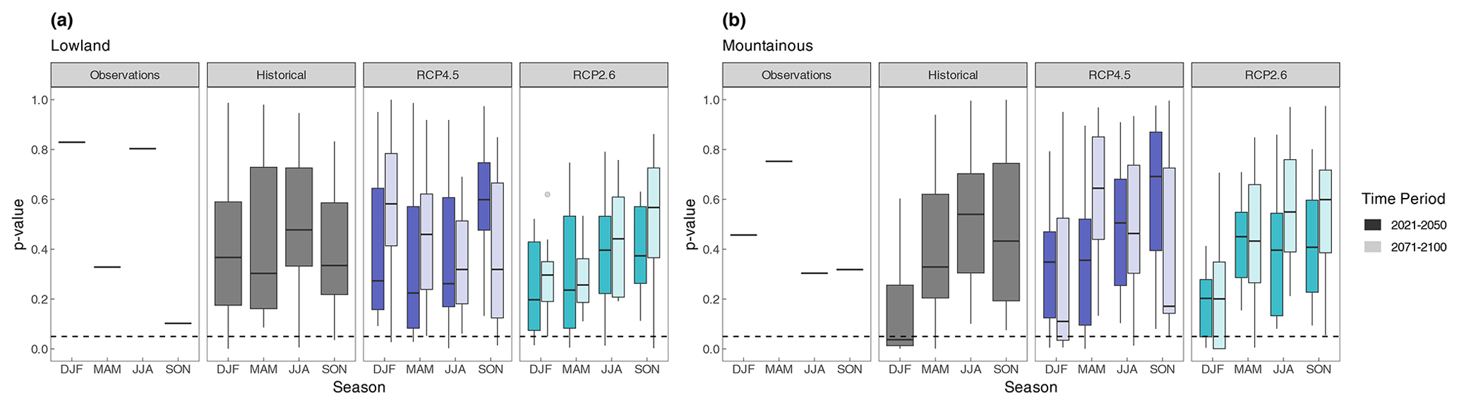
Figure 2 The p values of the Shapiro–Wilk test for normality considering seasonal CWB values for (a) lowland and (b) mountainous areas for observations (based on SPARTACUS and ARET data) shown as short segments and the historical runs of the selected RCMs as well as for scenarios RCP4.5 and RCP2.6 for the near future (2021–2050) and the far future (2071–2100) displayed as boxplots denoting for the distribution among the different model realizations.

The calculation of CWB return periods follows the general approach of statistical frequency analysis, where a theoretical distribution is fitted to the empirical distribution of the data to provide a robust estimate of the probability of events. As the CWB is a random variable which is unbound in the direction of both extremes, we assume a normal distribution to be a reasonable model. The model is fitted using the L-moments approach, which provides a robust estimate of model parameters in the case of outliers and observation uncertainty (Hosking, 1990).

We tested the assumption that the annual series of CWB indices (of different seasons, and stratified by lowland and mountainous areas) follow a normal distribution, using the Shapiro–Wilk test for normality (Shapiro and Wilk, 1965). The null hypothesis is that the data sample follows a normal distribution, p values below the 5 % threshold indicate that the null hypothesis is rejected, and the data come from another distribution.

The respective p values are displayed in Fig. 2 for the lowland (Fig. 2a) and the mountainous (Fig. 2b) areas for observations and RCM simulations. Considering the observations, the p values are mostly well above the 5 % levels; only autumn in the lowlands shows a p value closer to the significance threshold. Considering the climate simulations during the historical period, there is a considerable spread of p values among the different models, some of them even below the 5 % level. Particularly during winter in the mountainous areas in half of the model ensemble, the distribution is most likely not normal. However, in general median p values are range between 0.3 and 0.6, indicating normality for the majority of the model runs. During the scenario time periods, a similar picture emerges: median p values are way above the 5 % significance level. However, again in winter in the mountainous areas there is a considerable number of models with p values below the 5 % level. Although the CWB of some model runs most likely does not follow a normal distribution as observed, the majority of the simulations do and therefore enable a direct comparison of distribution features between the reference and future time periods. For the winter, higher uncertainties have to be taken into account.

Similar results are obtained assessing the stationarity of the different 30-year time periods considered, which is a general assumption of classical frequency analysis (Coles, 2001). We tested the observations as well as the climate scenario time periods for significant trends as an indication of non-stationarity. In the observations, none of the 30-year time periods investigated (for each season and for lowland and mountainous areas) show significant trends of the CWB following the Mann–Kendall trend test. These results are in line with similar investigations by Blöschl et al. (2018), who could show that increasing AED is balanced by an increase in precipitation. Considering the climate simulations, 13 % of all individual 30-year periods (576 in total as a result of 24 individual runs times 4 seasons times 3 time periods times 2 different areas) show significant trends at the 5 % level, thereby indicating non-stationarity. However, since this is only a minor fraction, and 30-year time slices are relatively short for assessing the stationarity of climate simulations, we consider classical extreme value theory to be generally applicable, while the related uncertainties are taken into account when interpreting the results.

To assess changing probabilities of extreme drought events under climate conditions, we examine future changes on return periods for a given event threshold. At first we use a 10-year event return period under historical climate conditions as a reference. We fitted a normal distribution to the historical climate simulations using L moments to obtain the distribution parameters. Then the same procedure is carried out for the future climate simulations; however this time we used the 10-year event threshold from the reference period to estimate the return period for this event from the fitted distribution. This yields the change in return period of a 10-year event and future climate conditions. We applied the same method for assessing the change in event return period of the 2003 summer drought event. This severe event is still a benchmark in terms of severity considering the past centuries (Laaha et al., 2017; Haslinger et al., 2019a; Haslinger and Blöschl, 2017; Ionita et al., 2017).

4 Results

4.1 Future change in average climatic water balance conditions

Average annual and seasonal CWB values over the Austrian domain from observations and respective CC signals are summarized in Table 2. During the reference period 1981–2010, the annual CWB from observations is +466 mm yr⁻¹; in winter the lowest values are apparent (+42 mm per season) due to lower precipitation rates in general and the build-up of the snowpack. In the transition seasons spring and autumn, values are rather similar with +110 and 133 mm per season respectively. The largest values of the CWB are apparent during summer, with an average of +181 mm per season.

Table 2 Climate change signal of the climatic water balance, average values over the Austrian domain and ensemble spread (1 SD – standard deviation of the ensemble distribution) on a seasonal (winter: DJF, spring: MAM, summer: JJA, autumn: SON) and annual (ANN) basis.

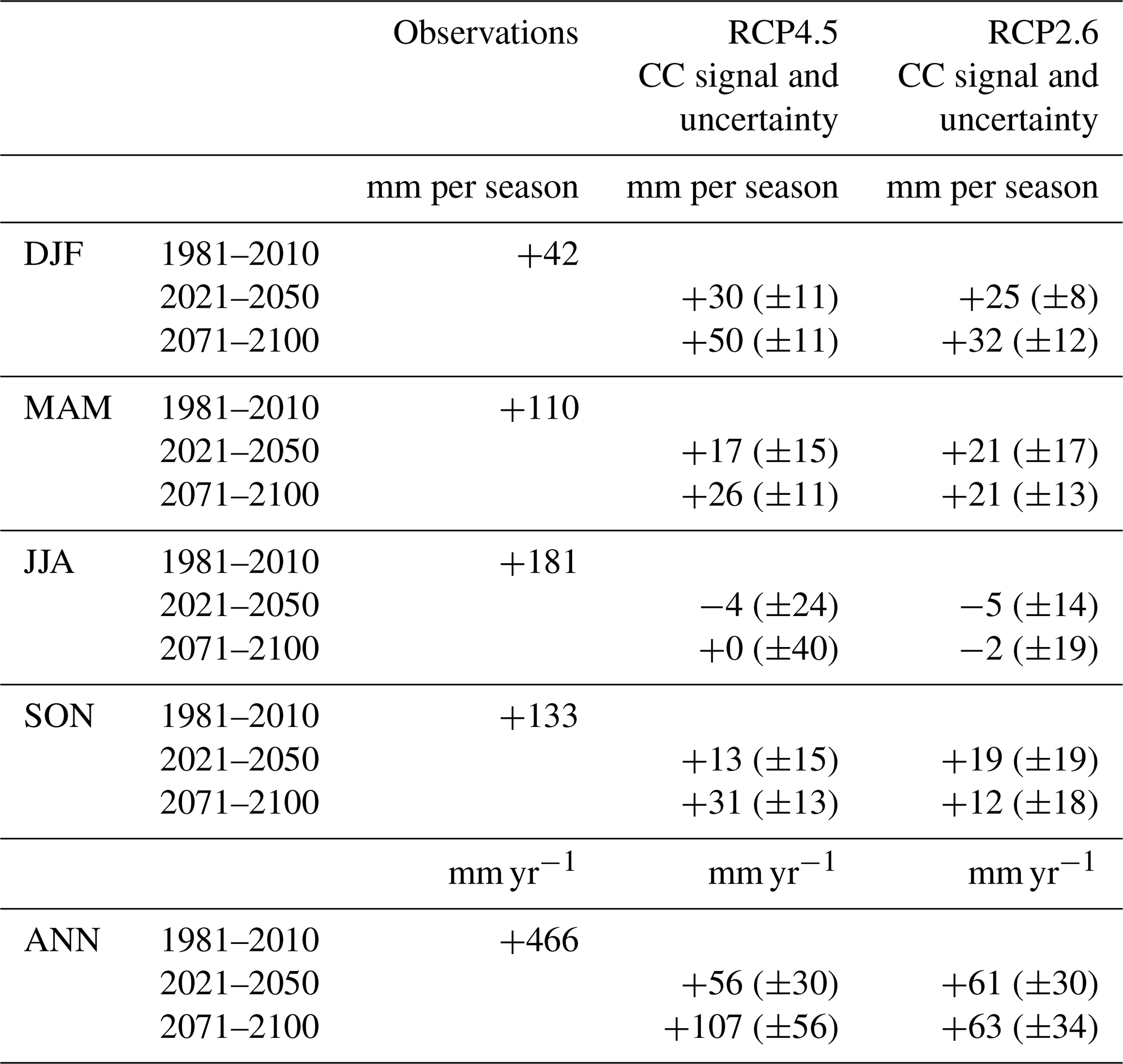
For future periods the CWB is expected to increase in winter, with a larger increase for RCP4.5 (+30 mm per season in the near future and +50 mm per season in the far future) compared to RCP2.6 (+25 mm per season in the near future and +32 mm per season in the far future). An increase is projected for spring as well, ranging between +17 and +26 mm per season in RCP4.5 for near and far future respectively; these values are equal to +21 mm per season for RCP2.6 in both future time periods. For these two seasons the ensemble spread is ranging roughly between 10 and 17 mm per season. For summer the CC signal is rather small, −4 and 0 mm per season for both periods respectively in RCP4.5 compared to −5 and −2 mm per season in RCP2.6. Contradicting this, the uncertainty of this CC signal is rather large given the wide range of the ensemble spread, which is specifically large in RCP4.5, reaching CC signals of ±40 mm per season during the far-future period. The ensemble spread is much smaller in RCP2.6, which might also be related to the smaller number of individual model runs, but still the ensemble spread is one-half to one-third of the RCP4.5 spread. Autumn is showing a moderate increase of the CWB with +13 and +31 mm per season for RCP4.5 and the near- and far-future periods and +19 and +12 mm per season for RCP2.6 respectively.

On an annual basis the simulations project a wetter future. CWB will increase by +56 and +107 mm yr⁻¹ for the near and future time periods respectively under RCP4.5, while under RCP2.6 these values are somewhat lower at +61 and +63 mm yr⁻¹.

A spatial assessment of the CC signal of the CWB as well as its components (rainfall, snow melt and atmospheric evaporative demand) for both emission scenarios and future time periods is given in Fig. 3. The changes in the CWB (Fig. 3a) are rather heterogeneous in space, creating a diverse pattern. Under RCP4.5 in the near future, we see slightly increasing CWB north of the main Alpine crest, whereas in the southern parts of the domain there is an apparent signal of decreasing CWB. This signal shifts towards the end of the century towards increasing CWB mostly over the entire domain, with exceptions in the western central alpine parts of Austria. RCP2.6 shows a somewhat different response, with increasing CWB throughout the domain in the near as well as in the far future. Exceptions here also include some parts in the westernmost areas of Austria showing slightly decreasing CWB.

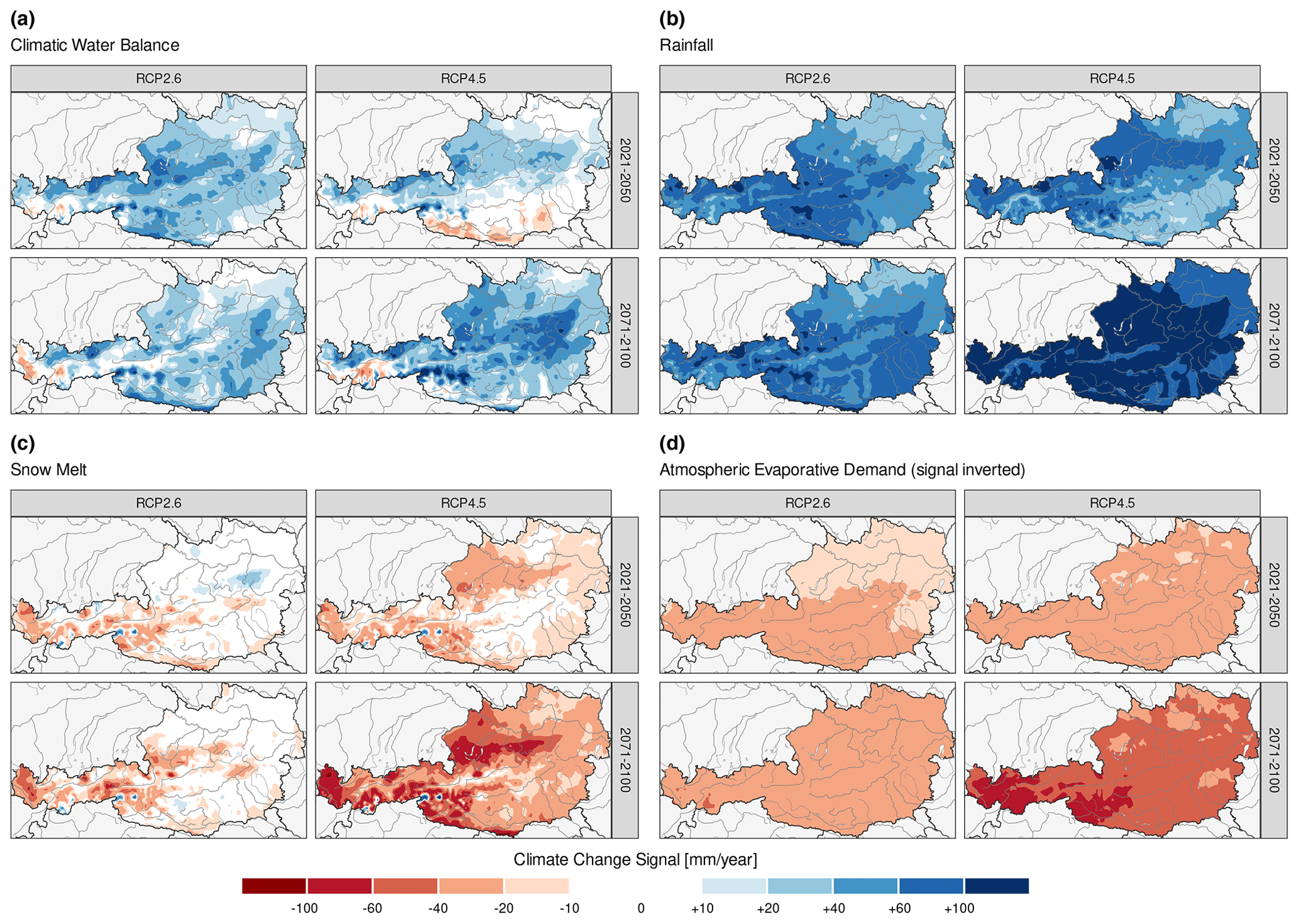
Figure 3 Median ensemble climate change signal of RCP4.5 and RCP2.6 for the near future (2021–2050) and the far future (2071–2100) of (a) the mean annual CWB and (b–d) the mean annual components of the climatic water balance: (b) liquid precipitation, (c) snow melt and (d) AED (note that the signal is inverted; negative values indicate an increase in AED).

Figure 3b shows the spatial patterns of changes in rainfall (liquid precipitation), which generally increases across both scenarios and both future time periods. However, subtle differences are apparent. For example, in RCP4.5 the increase in rainfall is larger by the end of the 21st century compared to the near future. Whilst the southern areas show smaller CC signals in the near future, this is no longer the case for the far-future period. On the other hand, in RCP2.6 the CC signal does not change significantly over the 21st century.

For the changes in snow melt, rather different patterns emerge, as displayed in Fig. 3c. The overall temperature increase following future global warming leads to a subsequent reduction in snow melt. This is caused by a decreasing fraction of solid precipitation compared to the total precipitation sums and therefore a decreasing snowpack, which in turn leads to declining snow melt. This CC signal is more pronounced in RCP4.5 following the stronger temperature increase. Considering spatial patterns, largest decreases are found in the Alpine fringes where precipitation in absolute terms is also the highest (cf. Fig. 1c). Only in the high-alpine areas along the main alpine crest does snow melt increase, which is due to generally increasing precipitation and meteorological conditions still cold enough to build up a persistent snowpack during winter. In RCP2.6 these changes are similar in their spatial pattern, although smaller. There is nearly no CC signal in the lowland areas in the near and far future. Exceptions are some subtle increases in some eastern mountainous areas, which are most likely due to increasing total precipitation in the region.

The CC signal of AED, as displayed in Fig. 3d, shows a more homogeneous pattern in space than the other variables. Smaller increases are visible in RCP2.6 due to the smaller temperature forcing. On the other hand, the signal is stronger in RCP4.5 with a slightly stronger signal in the mountainous areas.

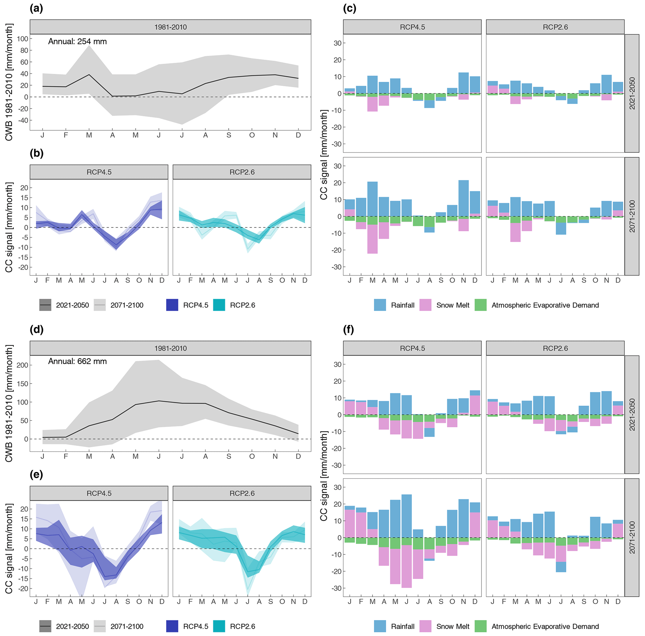
Figure 4 Monthly climate change signal of the CWB for lowlands in the upper panels and mountainous areas in the lower panels: (a, d) observed average monthly CWB in the reference period 1981–2010, where the shading denotes the spatial variability of the CWB climatology; (b, e) ensemble median monthly climate change signal of the CWB for RCP4.5 (blue) and RCP2.6 (turquoise) for the near future in bold colour and the far future in pale colour, where the shading denotes the ensemble spread given by the 10th and 90th percentiles; and (c, f) ensemble median monthly climate change signal of the individual CWB terms. Rainfall is denoted in blue, snow melt in magenta and AED in green.

In the light of this spatial assessment of changes in average CWB and its components, it is important to consider seasonal variations of change as well. Figure 4 shows these with regards to lowland and mountainous areas. The results for lowland areas are summarized in Fig. 4a–c, where Fig. 4a displays the spatially averaged monthly mean CWB during the reference period 1981–2010 based on observations. It shows somewhat larger values during winter and autumn with a small snow-melt-induced peak in March, and lower values are apparent from May to August. On average on an annual basis, the CWB is +254 mm yr⁻¹ in the lowlands. Considering future CWB changes (Fig. 4b), there is a mostly coherent CC signal of increasing CWB during the cold-season months for both time periods and emission scenarios. An exception is early spring (March and April), where a negative CC signal is visible under RCP2.6 in the far future. Positive CC signals are apparent during the beginning of the warm season (May and June) as well, particularly under RCP4.5 (both time periods) and RCP2.6 (far future) scenarios. On the contrary, negative CC signals appear during July, August and September (both time periods and emission scenarios), which are the largest mostly in August (−5 to −10 mm). The contributions to these changes from the individual terms of the CWB equation are displayed in Fig. 4c. Two things are obvious at first sight: on the one hand larger changes during the far-future period and on the other hand slightly larger changes for RCP4.5 (although foremost during the far-future period). The largest changes are apparent for rainfall. Here, a positive CC signal is seen during all months (largest during spring and autumn) except for July to September, where negative CC signals are visible to some extent. Seasonally punctuated changes are visible for snow melt, where positive changes are visible in the winter months (December, January, and February) and negative deviations mostly during spring. These are most likely caused by seasonally shifted snow accumulation and ablation processes with higher temperatures causing earlier snow melt, which is lacking during those months where snow melt mostly occurred in the reference period. Reasons for increasing snow melt during winter might arise from higher temperatures as well, causing snowpacks to more often melt during the winter months in future time periods than was observed in the reference periods. In contrast to these rather large changes of these two variables, the CC signal of reference evapotranspiration is rather small. It is of course the largest in the far future and RCP4.5, which shows a bigger temperature increase; however, the largest deviations are −5 mm per month for July (RCP4.5, far future), which is considerably smaller than changes in rainfall and snow melt (up to +20 mm per month).

As is visible from Fig. 4b the CC signal of the CWB is nearly zero for early spring (March and April); however, considering the individual terms of the climate water balance, huge dynamics are apparent with a considerable shift from snow melt to rainfall during this time of the year. Positive CWB signals are mainly caused by increasing rainfall, particularly during winter. On the contrary, the negative CWB changes during summer are caused by both increasing AED and slightly decreasing rainfall.

Considering the mountainous part of Austria (Fig. 4d–f), there are completely different climatological initial conditions. Figure 4d displays the average monthly CWB, which depicts an inverted annual evolution compared to the lowlands (cf. Fig. 4a) with the lowest values during winter (slightly above zero) and the largest values during summer (maximum in June, +100 mm). These low values during winter are mainly caused by strongly reduced positive moisture flux from rainfall and snow melt, since precipitation appears mostly in the form of snow which is accumulated and later in the year released through snow melt. These snow melt processes along with increasing precipitation sums in the warm season add up to the peak appearing in summer. On average the observed CWB on an annual basis is +662 mm yr⁻¹.

The CC signal of the CWB is displayed in Fig. 4e. For both scenarios and both future time periods, a similar pattern is apparent, showing increasing CWB during the cold season, particularly during winter. Differences arise during spring, where RCP4.5 is showing no clear change, whereas in RCP2.6 an increase is visible as large as during the winter months. Common in both scenarios is the distinct negative CC signal during July and August where negative deviations between −10 and −15 mm per month occur. The patterns of change of the individual terms of the CWB are depicted in Fig. 4f.

In general, these patterns are similar to the lowlands; however the magnitude of the CC signal is much larger and there are also larger changes for RCP4.5 and the far-future period. The mountainous areas show a pronounced increase in rainfall similar to the lowlands, with highest CC signals from May to June and October to November. As for the lowland areas slightly negative changes are visible in the summer months. In the higher-elevation regions the impact of snow accumulation and ablation is far bigger compared to the lowlands; hence there are considerable changes in snow melt apparent over the course of the year. In particular there is an increase in snow melt from December to March, again the largest in RCP4.5 and for the far future. During the remaining months the future CC signal is negative, most pronounced during June and July. This points to a shift of the strongest seasonal CC signal between lowland and mountainous areas. Here the signal is stronger later in the year, along with a generally later melting season. As for the lowland areas the contribution of changes in AED is small compared to the rainfall and snow melt components and is within a range of −5 to −10 mm per month during the summer months.

Given this detailed analysis of future changes of the individual components of the CWB in lowland and mountainous areas, it is apparent that snow melt changes may exhibit the largest changes across seasons and elevation bands. To shed more light on this matter, Fig. 5a shows exemplarily the CC signal of snow melt for RCP4.5 and the far future for the individual months and from 200–3400 m a.s.l. elevation. Here we see a general increase in snow melt during winter (DJF) between 500 and 2000 m a.s.l. of 10–20 mm per month. However, the CC signal in both the negative and positive direction is getting stronger during spring and summer. A distinct dividing line along season and elevation is apparent, separating elevations with negative and positive snow melt CC signal. The magnitude increases as well with elevation, which is due to the increasing total precipitation sums at higher elevations. For every point in time of the spring–summer season, there is a critical level of elevation with zero change and positive CC signal above that and vice versa. Increasing snow melt above the critical elevation is caused by both increasing precipitation during winter and spring and higher temperatures causing more snow melt than in the reference period. On the other hand, decreasing snow melt below the critical elevation is due to thinner snowpack following decreasing snow accumulation during winter and a higher rainfall fraction along increasing temperatures.

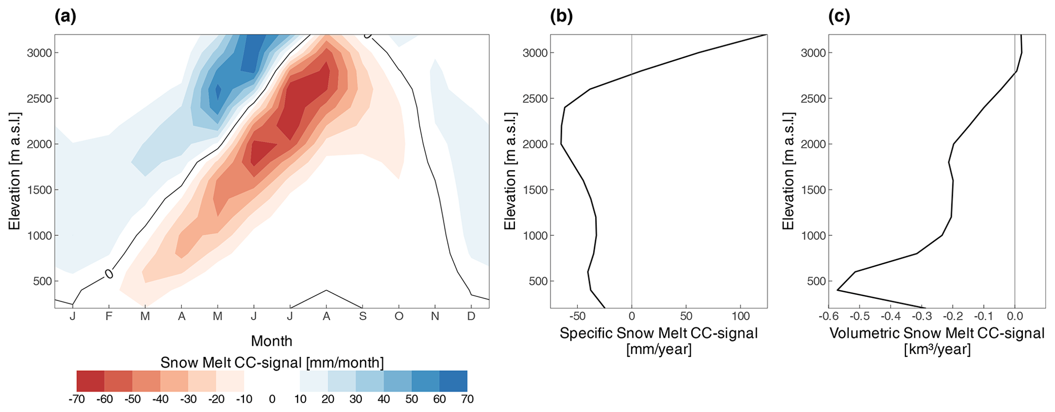
Figure 5 (a) Snow melt CC signal depending on time of the year (month) and elevation for RCP4.5, 2071–2100, (b) averaged over all months and (c) given as volumetric change (multiplied by area of elevation class).

On average over the course of the year (Fig. 5b) snow melt is decreasing up to 2700 m a.s.l.; higher up, snow melt increases. This pattern is driven by increasing temperatures leading to less snow accumulation, particularly in lower elevations. However, the signal changes at higher elevations (>2700 m a.s.l.) where snow melt is increasing. This is due to the increasing total precipitation amount during winter and still low enough temperatures to build up a significant snowpack, which is the reason for the positive snow melt signal. Assessing these changes in a volumetric perspective (multiplying by the areal extent of the elevation band) gives a rather different picture (Fig. 5c), where the largest changes are found below roughly 700 m a.s.l., due to the larger spatial extent, highlighting that these areas are most sensitive to snow melt changes in absolute terms.

A special case in this assessment of CWB changes across Austria is the spatial domain of the high-alpine areas (>2500 m a.s.l.) due to the considerable fraction of these covered with glaciers. The seasonal evolution of the CWB in the high-alpine domain is displayed in Fig. 6a. During the cold season from November to April–May, the CWB is slightly negative. Most precipitation occurs in the form of snow, consequently building up the snowpack, which acts as a storage term for the summer months. The slightly negative values during winter are due to the small but steady losses due to AED. However, from May onwards the snow melt season sets in and also the fraction of liquid precipitation increases, leading to a steep rise of the CWB until its peak in July (+200 mm per month) before it approaches zero again in October. The average CWB is 413 mm yr⁻¹.

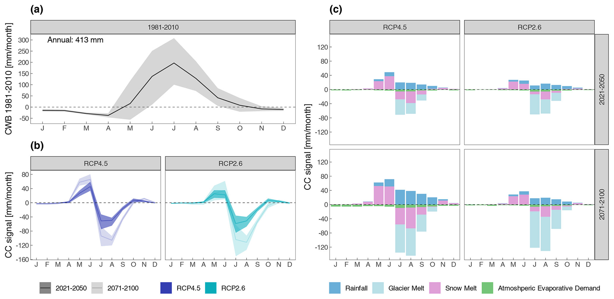
Figure 6 Monthly climate change signal of the CWB for the high-alpine areas: (a) observed average monthly CWB in the reference period 1981–2010, where the shading denotes the spatial variability of the CWB climatology, (b) ensemble median monthly climate change signal of the CWB for RCP4.5 (blue) and RCP2.6 (turquoise) for the near future in bold colour and the far future in pale colour, where the shading denotes the ensemble spread given by the 10th and 90th percentiles, (c) ensemble median monthly climate change signal of the individual CWB terms. Rainfall is denoted in blue, snow melt in magenta and AED in green.

Future changes of the high-alpine CWB are displayed in Fig. 6b. The patterns are similar in both scenarios, showing hardly any change until May, where positive CC signals are visible. The CC signals become strongly negative during July, August and September and are only minor for the rest of the year. A major difference compared to the lowland and mountainous change patterns (cf. Fig. 4b and e) is the stronger CC signal during the far-future period. In the high-alpine area the CC signal is more pronounced than in the lowland and mountainous areas. The reduction of the CWB is around −100 mm per month for July and August for the far-future period, which is a reduction of 50 % compared to the CWB in the reference period 1981–2010 (cf. Fig. 6a).

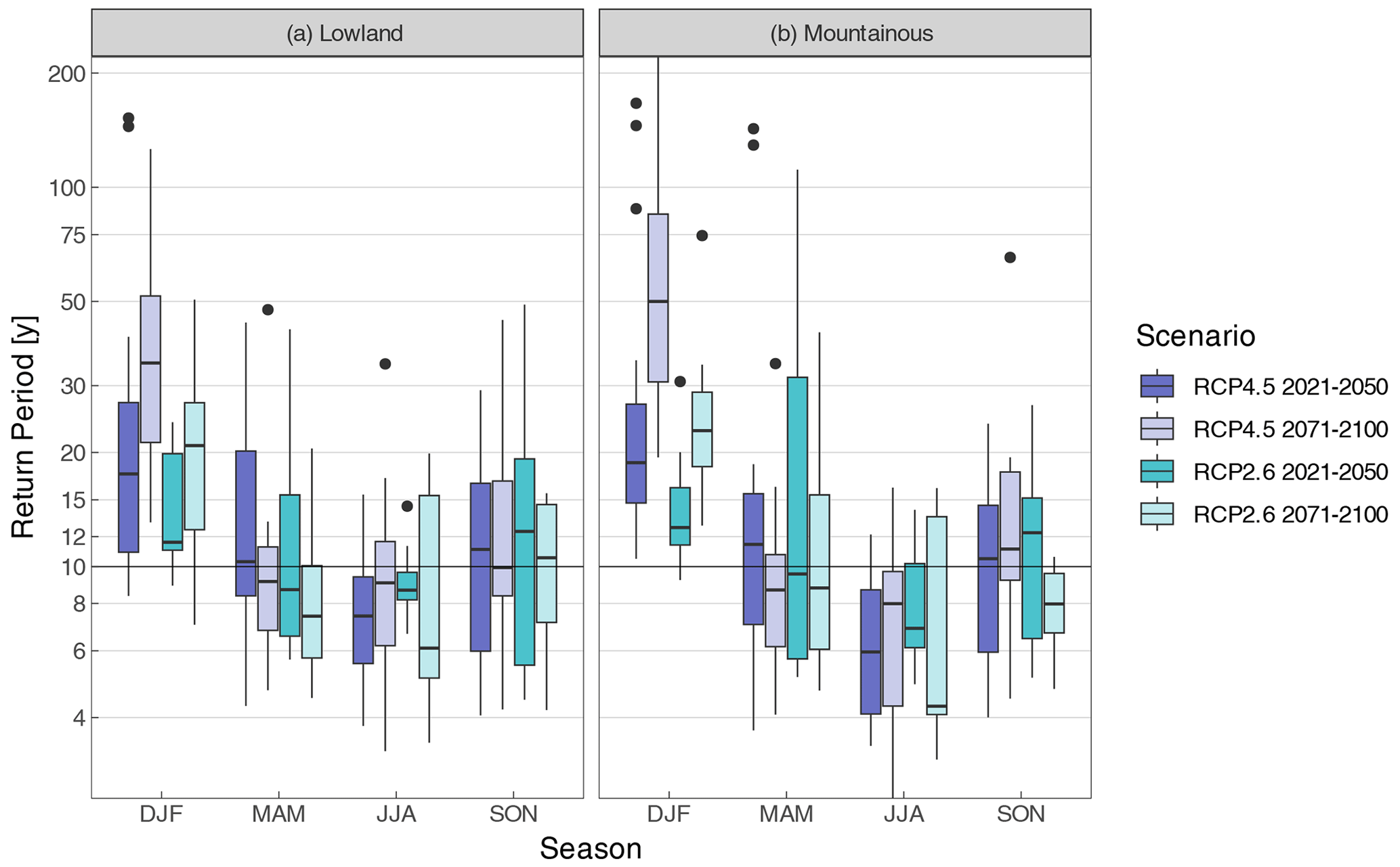
Figure 7 Change in return period of a CWB 10-year event in the reference period (1981–2010) for lowland (a) and mountainous areas (b) under RCP4.5 (blue) and RCP2.6 (turquoise) for the near future (2021–2050, bold colours) and the far future (2071–2100, pale colours). The boxplots denote the ensemble spread of the individual climate model runs.

The reason for these large changes is revealed by examining the change of the individual components of the CWB (Fig. 6c). In addition to the three main components of the CWB (rainfall, snow melt and AED), we consider glacier melt for the high-alpine areas as well (see Sect. 3.4 for details). From May to October an increase in rainfall contributes positively to the CWB CC signal, which is the strongest in RCP4.5 in the far future with +40 mm per month in July and August. In addition, snow melt increases during May. On the other hand, snow melt is decreases considerably from June to September, again most pronounced in RCP4.5 in the far-future period. This pattern resembles that of the mountainous areas, although the peak of the negative CC signal is in August for the high-alpine area. Similar processes cause these changes, namely reduced snowpack during summer due to earlier ablation under a warmer future climate. The most important driver of the negative CC signal of the CWB is the change in glacier melt. It is the largest contributor from July to September and shows the largest signals in the far future. Continued warming leads to sustained ice loss, which produces increasing runoff after initial temperature increase. However, once a critical threshold (commonly referred to as “peak water”) is exceeded, the runoff decreases due to the shrinking ice volume of the glaciers. By the near-future period this threshold is most likely surpassed by all glacier-covered areas in Austria; thus, decreasing glacier runoff is a consequence of further future warming (e.g. Huss and Hock, 2018; Pepin et al., 2022).

4.2 Future change in extreme drought event probabilities

Apart from assessing changes in the mean state of the CWB and its components on an annual and seasonal basis, it is important to quantify changing probabilities of drought events of a certain threshold. As described in more details in the Methods section, we define a moderate drought event where the CWB is below the 10-year return period threshold during the reference period 1981–2010. Now we estimate the return period of this given reference threshold for future climate conditions.

The results on a seasonal basis and stratified by lowland and mountainous areas are displayed in Fig. 7. For winter an increase in return period (lower probability of drought occurrence) is given across all scenarios, time periods and elevation areas. However, the signal is stronger in RCP4.5 with a median return period across all models of around 20 years (lowland and mountainous areas) for the near future and 30 years for the lowland (50 years for mountainous) areas for the far future. The signal in RCP2.6 is less pronounced with future return periods between 12 years (near future) and 20 years (far future), similar across lowland and mountainous areas.

Only subtle changes are apparent in spring. Here the median future return periods are only marginally lower, particularly under RCP2.6 in the lowlands. During summer, median return periods for the given threshold generally decrease in both future time periods, scenarios and elevation regions. However, the signal is more robust in the near future, due to smaller ensemble spread. Here median return periods between 7 years (RCP4.5) and 9 years (RCP2.6) for the lowland areas and 6 years (RCP4.5) and 7 years (RCP2.6) for the mountainous areas are apparent. For the far future, uncertainty increases as depicted by increasing ensemble spread, and median return periods range between 8 and 6 years in the lowlands and 8 and 4 years in the mountainous areas.

In autumn no clear change signal is visible. Median return periods marginally increase in both time periods, scenarios and elevation areas (one exception is RCP2.6 in the far future in mountainous areas). However uncertainties are again large due to substantial ensemble spread.

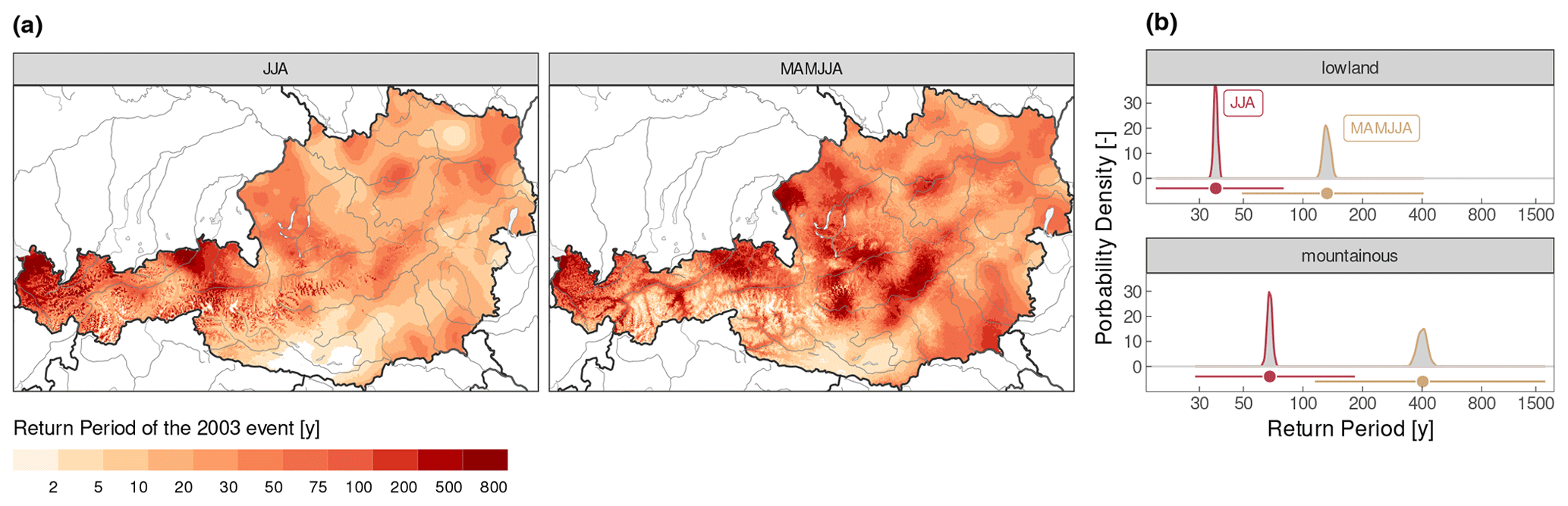
Figure 8 (a) Spatial estimate of the 2003 event return period for summer (JJA) and spring and summer (MAMJJA) based on the observed CWB distribution in the reference period 1981–2010, (b) uncertainty assessment of the return period estimates. Density plots denote the uncertainty from spatially averaging. A bootstrapping approach with 1000 iterations randomly sampling 10 % of the respective grid points in the region and averaging afterwards is applied. Point-range plots denote the uncertainty from distribution fitting of the randomly sampled spatial averages. The range denotes the full range of iterations and the dot the median of the iterations for return period estimates.

The projected changes point towards subtle decoupled signals of the mean change and changes in the tails of the distribution. While there is no clear sign for changes in the mean CWB values in summer (cf. Table 2), we see here some evidence for increasing probabilities of moderately extreme drought conditions during summer. To examine the future risk of extreme drought conditions in more detail, we analyse the drought event of the year 2003 in the light of its return period for past climate conditions and future projections. This event was extraordinary in terms of its magnitude, spatial extent and impact (Black et al., 2004; Schär and Jendritzky, 2004; Fischer et al., 2007); apart from other events that struck Austria in recent years (drought of 2015, e.g. Laaha et al., 2017, Ionita et al., 2017; and the drought of 2018, e.g. Buras et al., 2020), the event of 2003 impacted Austria nearly entirely. Other reported events affected only the northern parts of the country, highlighting the prominent dipole structure of drought events in the Alpine region (Haslinger and Blöschl, 2017; Haslinger et al., 2019b). In a first step we assess the severity of the event by estimating the return period of the CWB for summer (JJA) as well as for spring and summer (spring–summer, MAMJJA). Several publications have highlighted the special precondition of the extraordinary dry spring, which most likely intensified the consequent summer drought and heatwave (Haslinger et al., 2019a; Laaha et al., 2017; Fischer et al., 2007). This is why we chose to analyse the summer season and the spring–summer season separately.

Figure 8a displays the grid-point-wise estimation of the 2003 event return period of the CWB for summer and spring–summer for the reference period 1981–2010. The maps indicate a higher severity if spring–summer is considered, which is also in line with other findings which claimed that the initialization of the drought was already in March (Haslinger and Blöschl, 2017; Fischer et al., 2007), starting the warm season with a considerable moisture deficit. Also common in both maps is the higher severity in the western and northern parts of the country; the southernmost part was not that severely struck, particularly if only summer is considered.

When deriving spatial averages for the lowland and mountainous areas of these return periods, we assess the uncertainty arising from spatial averaging and from distribution fitting. The results are shown in Fig. 8b. The two panels show the uncertainty assessment for the lowland and the mountainous areas, where the kernel densities display the uncertainty from spatial averaging and the point range for the distribution fitting. In general, the uncertainty from the fitting is much larger compared to the spatially averaging, which is true for both areas. For the lowland areas the spatial uncertainty is between 34 and 38 years (117 and 152 years) for summer (spring–summer), and for the mountainous areas it ranges between 62 and 73 years (322 and 500 years) for summer (spring–summer). The uncertainty from distribution fitting is considerably larger. Here for the lowland areas the estimates range between 18 and 90 years (50 and 400 years) for summer (spring–summer) and for the mountainous areas between 29 and 183 years (115 and 1673 years) for summer (spring–summer). The best estimate for the lowland areas is 36 years (132 years) for summer (spring–summer) and for the mountainous areas 68 years (403 years) for summer (spring–summer).

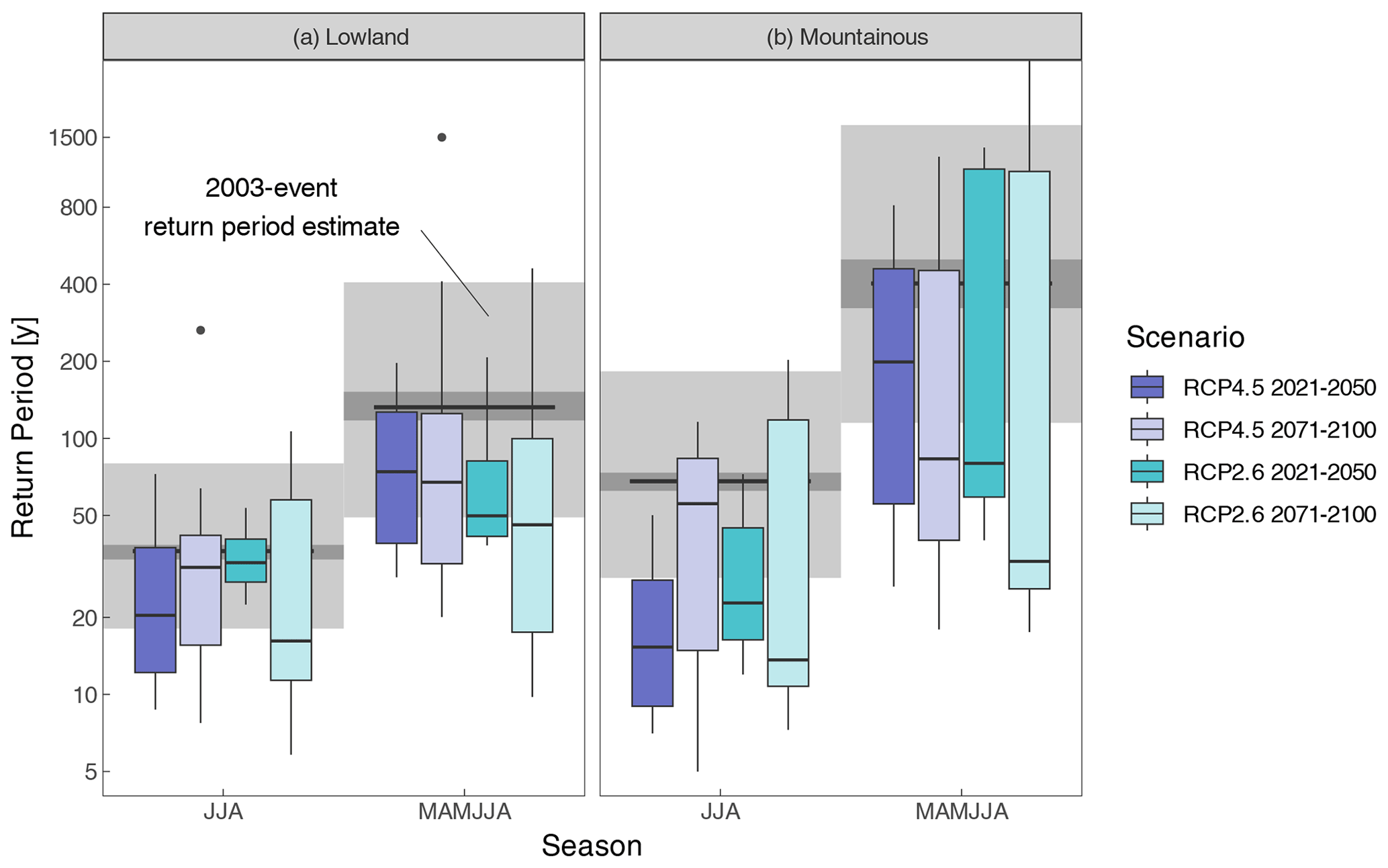
Figure 9 Future return period estimate of a drought event with a 2003 event threshold for lowland (a) and mountainous areas (b) under RCP4.5 (blue) and RCP2.6 (turquoise) for the near future (2021–2050, bold colours) and the far future (2071–2100, pale colours). The boxplot denotes the ensemble spread of the individual climate model runs. The grey areas indicate the uncertainty from observed return period estimates (cf. Fig. 8b) in the reference period 1981–2010, where the darker shades indicate the spatial averaging uncertainty and the lighter shading the distribution fitting uncertainty.

Similar to the previous analysis of future return periods of a 10-year event in the reference period, we assess the return period for a 2003 event under future climate conditions (Fig. 9). For the lowlands in summer there is a reduction in return period visible. Under RCP4.5 the ensemble median is around 20 years for the near future and higher in the far future, compared to 36 years in the reference period. Under RCP2.6 there is a reduction in return period (ensemble median) to 33 years (16 years) in the near future (far future). The decrease in return period is visible in the mountainous areas in summer as well with a drop to 16 years (56 years) in the near future (far future) under RCP4.5. Under RCP2.6 the reduction is similar. Here values of roughly 23 years (14 years) are apparent for the near future (far future). For lowlands in the combined spring–summer season (MAMJJA), changes are larger to some extent. The ensemble median is around 70 years for the near future and far future respectively under RCP4.5 and around 50 years for the near and far future respectively under RCP2.6. For the mountainous areas in spring–summer, the ensemble median return period ranges between 200 (RCP4.5, near future) and 33 years (RCP2.6, far future). In general, uncertainties expressed via the ensemble spread increase with the time horizon (larger for far-future estimates) and are larger for the combined spring–summer season and the mountainous areas. This might be related to the complex nature or drought-generating processes in snow-dominated areas, here particularly during spring and the mountainous part of the country.

The probability of a rather extreme event like 2003 strongly increases under future climate conditions, which is the case for all time periods and emission scenarios indicated by a median return period in future time periods well below the best estimate of the 2003 event return period in the reference period. It also seems that the model agreement is stronger at this even more extreme region of the CWB distribution, since the return period of the 2003 best estimate is often outside the interquartile range (“box” of the boxplots). This feature is not as clear for the 10-year event return period change (cf. Fig. 7) for summer.

In the light of the minor seasonal CC signals and an increase in probability of reaching extreme dry conditions, these results point towards a general increase in (interannual) variability of the CWB, particularly during summer (and spring), as this season is examined in more detail here.

However, to quantify potential changes in the interannual variability of the CWB, the changes in standard deviation of summer and spring–summer CWB values for the lowland and mountainous areas are calculated for future climate conditions compared to the reference period. The results are displayed in Fig. 10. As expected, the ensemble median change of the interannual variability across both seasons, scenarios and time periods increases. One exception is RCP2.6 for the near-future summer season; here a slight decrease is visible. Although the uncertainties are large, given the wide range of the individual boxplots, the climate scenarios consistently point towards a more variable future on an interannual timescale and therefore an increasing probability of experiencing extreme hydrometeorological states. This alterations of the climate systems and the implications for drought hazard risk are shown in other studies. For example, Ukkola et al. (2020) showed that increasing interannual variability of precipitation is the main driver of drought risk in central Europe. On the other hand, declining mean precipitation drives increasing drought probabilities in the Mediterranean region.

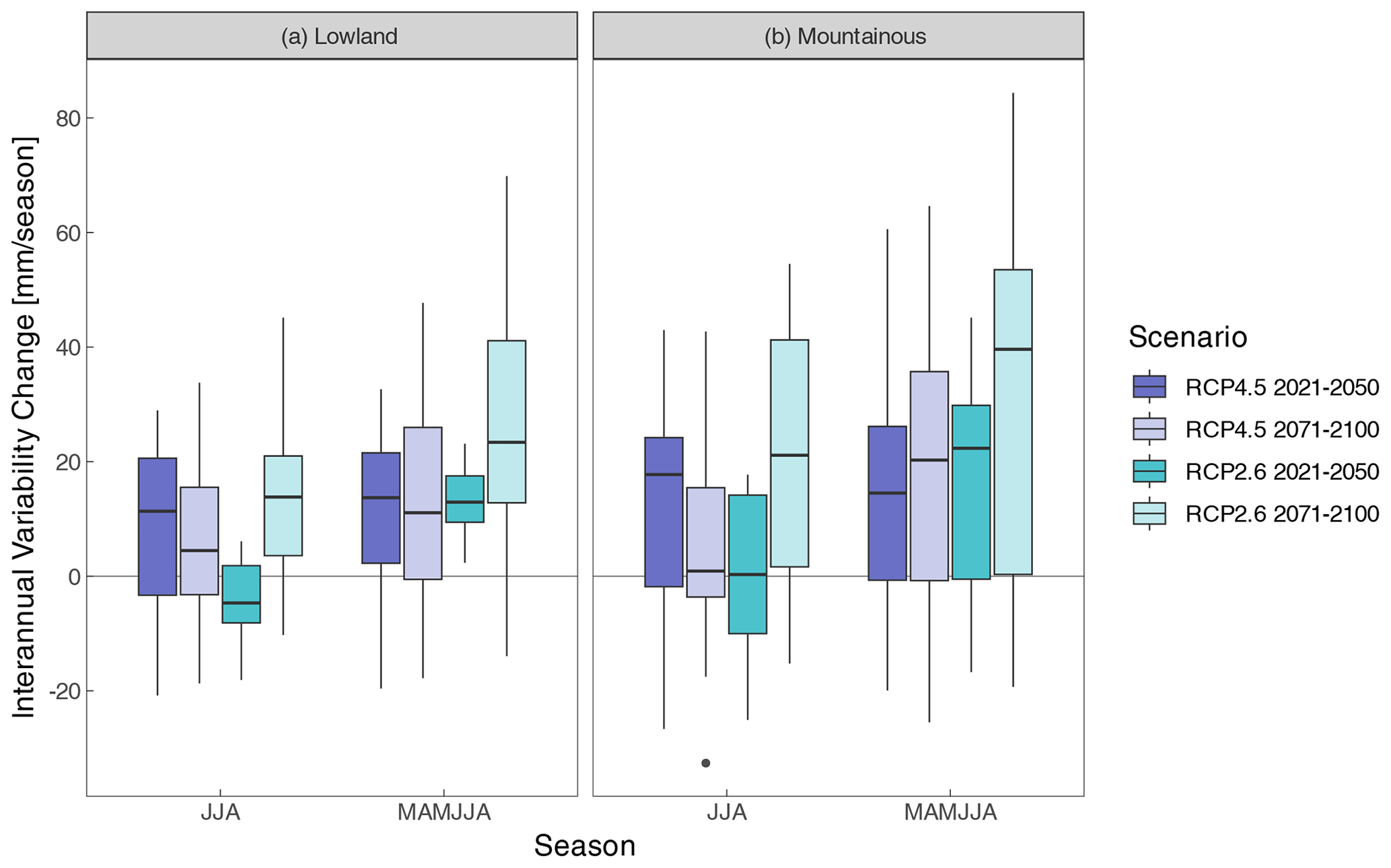
Figure 10 Future change in interannual variability of seasonal CWB for lowland (a) and mountainous areas (b) under RCP4.5 (blue) and RCP2.6 (turquoise) for the near future (2021–2050, bold colours) and the far future (2071–2100, pale colours). The boxplot denotes the ensemble spread of the individual climate model runs.

5 Discussion

In this study future surface water availability in the complex terrain of the Austrian domain is investigated as a function of elevation and climatic water balance components. Using two emission scenarios we found similar spatial patterns of the CC signals across the various variables investigated, although these are slightly stronger in the moderate mitigation scenario RCP4.5 due to larger temperature forcing. Here we use downscaled and bias-corrected climate scenarios (RCP2.6 and RCP4.5) of the EURO-CORDEX initiative based on a tailored CMIP5 ensemble of global climate models. We intentionally do not use an extreme emission scenario like RCP8.5, as the literature is growing on the implausible exaggeration of future emissions of this socio-economic pathway (see details in the data section). Although RCP4.5 might be seen as the most plausible scenario at current times, even larger global temperature increases cannot be completely discarded. Non-linear behaviour and the potential of crossing tipping points of the climate system may cause additional warming, leading to temperature levels far beyond current plausible scenarios like RCP4.5. Although the existence of some tipping points and moreover the timing of them in general are still under debate (Brovkin et al., 2021; Lenton et al., 2008), uncertainties in the climate system arising from this matter have to be kept in mind.

Compared to former studies considering future drought conditions in Austria, slightly different results are obtained. For example, Haslinger et al. (2016) and Laaha et al. (2016) assessed future SPEI trends based on RCMs driven by AR4 CMIP3 global climate models (GCMs). Here the authors found a general drying trend on an annual basis and for all seasons except for winter. This is contrast to our findings here, where the newer generation of models indicates wetter conditions in general on an annual basis and particularly wetter winters and springs. This increase in precipitation is a feature not only in this study using this specific model ensemble, but also in several others (Kotlarski et al., 2023). The origins of this trend towards more wetness in winter and spring is not fully understood. However, Rajczak and Schär (2017) point to the specific location of the Alpine region in a transition zone between future precipitation increase (decrease) on the northern (southern) side of the main Alpine crest.

In addition, we displayed future changes of the most important variables acting on the surface water availability. Apart from minor increases of AED, which are also shown in Gali Reniu (2017) for the same scenario dataset, the largest changes and shifts in seasonality are found for snow melt and the fraction of liquid precipitation. Our findings for Austria are in line with others considering different domains in the mid-latitudes (e.g. Musselman et al., 2021; Livneh and Badger, 2020, for the western United States) or from a global perspective with regards to agricultural drought (Qin et al., 2020). For the central European mountain ranges, the impact of snow melt changes on summer low flows was investigated by numerous studies (Meriö et al., 2019; Jenicek et al., 2018; Jenicek and Ledvinka, 2020) showing similar seasonal shifts. However, although some modelling uncertainties prevail (Olefs et al., 2020), we are confident that the presented results indicate robust snow melt CC signals given the projected precipitation and temperature changes.

In high-elevation areas the contribution of glacier runoff to surface water availability becomes increasingly important (Kaser et al., 2010). For Austria we could show that changes in glacier runoff denote the largest fraction compared to the other climatic water balance components in the high-alpine areas during the summer months. The largest negative changes are found in July and August, with positive changes, although smaller, occurring during May and June. This is in broad agreement with previous studies (e.g. Huss, 2011), which indicate that the so-called “peak water” is already surpassed or will be in the near future, which means that the shrinking glacier volume along with warming is yielding lower amounts of meltwater. Although the contribution of glacier melt to the overall water balance of large river basins in central Europe (e.g. Danube) is only minor during cool and wet summer season, it strongly increases during drought years, as particularly shown for the 2003 event (Huss, 2011). In the light of the results presented here, peak water in the wake and increasing drought hazard risk in the summer in future time periods are likely to stress low land water availability beyond experienced scarcities of the past.

Considering the occurrence of moderate (e.g. 10-year return period) and extreme (e.g. 2003 event) drought events in the future, the climate scenarios project an increase in return period (viewer events) during winter and no clear change in spring and autumn. However, during summer, a decrease in the return period (more events) of moderate and extreme droughts is projected across all scenarios, although the mean CC signal of the CWB is around zero. The change is rooted in the increase of interannual variability of future climate, which is observable during all seasons. Increasing CWB during winter, spring and autumn however compensates the signal of increasing variability. However, this is not the case for the summer season, where rising variability significantly lowers the return period of moderate and extreme droughts. These findings are confirmed by another recent study investigating drivers of future meteorological drought changes for central Europe (Ukkola et al., 2020). As thoroughly presented in Pendergrass et al. (2017), precipitation variability is expected to increase in a warmer climate across all timescales from days to decades. The authors pointed towards a nearly linear relationship between a temperature increase and the respective increase in atmospheric moisture content, precipitation variability and mean precipitation. Interestingly, variability change is in any case higher than a change in the mean, except for the winter season in the mid-latitudes, and thus it is a rather robust signal of future climate change.

Although the results presented here show a more or less linear response of surface water availability and drought occurrence with regards to warming levels, it is important to interpret these findings in the light of observed drought variability. Numerous studies point towards a significant contribution of multi-decadal climate variability in driving drought periods in the Alpine region and central Europe (Hanel et al., 2018; Moravec et al., 2019; Haslinger et al., 2019a, b). Internal variability of the climate system, predominantly in the North Atlantic Ocean, is found to particularly drive changes in atmospheric circulation and thus drought-favouring weather regimes over central Europe (Haslinger et al., 2021; Sutton and Hodson, 2005; O'Reilly et al., 2017). However, current state-of-the-art GCMs still fail to reproduce the main features of multidecadal climate variability in the Northern Hemisphere (O'Reilly et al., 2021; Kravtsov et al., 2018). This might be due to lacking spatial resolution of the ocean and atmospheric models (Caesar et al., 2018), a problem which could be overcome in the near future with increasing computational power. It is important to understand the presented results in the light of climate scenarios which are driven by a merely linear anthropogenic greenhouse gas forcing of different magnitude. The response of the climate system over the course of the 21st century is tied to this forcing and, as mentioned, lacks the ability to provide consistent multidecadal internal variability. To this end, it is very likely that multidecadal climate variability generates periods of excess on the one hand and even lower water availabilities on the other hand. Hence drought conditions and in addition further climate change shift seasonal regimes with the potential to drive water scarcity to unexpected levels.

6 Conclusion

In this study we presented scenarios of future surface water availability across different elevations and for the most important variables of the CWB. In general, wetter conditions are projected on an annual basis (e.g. RCP4.5 +107 mm, RCP2.6 +63 mm for the period 2071–2100). However particular seasonal shifts of snow melt and glacier melt at higher elevations change the surface water availability in the course of the year. Drought conditions in particular are expected to become more frequent during summer months, which is predominantly driven by an increase in interannual variability of the CWB. For a 2003-event-like situation during summer in the lowlands, the return period is estimated to decrease from 36 to 20 years under RCP4.5 in the near future for example. From the knowledge of past drought periods, it is important to highlight the role of internal climate variability, which is not well depicted by current climate models. The climate projections are to be seen as potential conditions under a quasi-linear climate forcing from greenhouse gases. For the adaptation to future drought conditions, it is therefore of utter importance to prepare for more extreme states of the climate system which are not depicted by current models. Local to regional efforts for storing water during times of excess and the re-cultivation of wetlands for example may be feasible measures in the short term, having the potential to mitigate severe drought impacts. However, a deeper understanding considering the driver on a local to hemispheric scale of future water availability is necessary to apply sufficient adaptation to potential drought conditions and water scarcity.