the Creative Commons Attribution 4.0 License.
the Creative Commons Attribution 4.0 License.
 | 01 Aug 2023
Joint probability analysis of storm surges and waves caused by tropical cyclones for the estimation of protection standard: a case study on the eastern coast of the Leizhou Peninsula and the island of Hainan in China
Zhang Haixia
Cheng Meng
Fang Weihua
The impact of natural hazards such as storm surges and waves on coastal areas during extreme tropical cyclone (TC) events can be amplified by the cascading effects of multiple hazards. Quantitative estimation of the marginal distribution and joint probability distribution of storm surges and waves is essential to understanding and managing tropical cyclone disaster risks. In this study, the dependence between storm surges and waves is quantitatively assessed using the extreme value theory (EVT) and the copula function for the Leizhou Peninsula and the island of Hainan of China, based on numerically simulated surge heights (SHs) and significant wave heights (SWHs) for every 30 min from 1949 to 2013. The steps for determining coastal protection standards in scalar values are also demonstrated. It is found that the generalized extreme value (GEV) function and Gumbel copula function are suitable for fitting the marginal and joint distribution characteristics of the SHs and SWHs, respectively, in this study area. Secondly, the SHs show higher values as locations get closer to the coastline, and the SWHs become higher further from the coastline. Lastly, the optimal design values of SHs and SWHs under different joint return periods can be estimated using the nonlinear programming method. This study shows the effectiveness of the bivariate copula function in evaluating the probability for different scenarios, providing a valuable reference for optimizing the design of engineering protection standards.
- Article
(14084 KB) - Full-text XML
- BibTeX
- EndNote


Tropical cyclone storm surges and waves could cause severe loss of life and property in offshore and coastal areas (Chen and Yu, 2017; Marcos et al., 2019; Wahl et al., 2015), and it is of great importance to quantify the intensity–frequency relationship of storm surges and waves, in order to understand the joint severity of multi-hazard extreme tropical cyclones (TCs; Zhang and Wang, 2021; Galiatsatou and Prinos, 2016).
In the past, many studies have analyzed single hazard indicators of tropical cyclone storm surges and waves (Lin et al., 2010; Shi et al., 2020; Teena et al., 2012), often with observed time series data or with simulated results by numerical models (Petroliagkis et al., 2016; Bilskie et al., 2016; Huang et al., 2013; Papadimitriou et al., 2020). The intensity values of the surge height (SH) or significant wave height (SWH) of a specific return period can be estimated based on the extreme value theory (EVT) (Teena et al., 2012; Muraleedharan et al., 2007; Morellato and Benoit, 2010; Niedoroda et al., 2010). Accordingly, the estimated probabilities of single hazards, such as SH or SWH, have been widely applied in the protection standard in coastal areas (Bomers et al., 2019; Perk et al., 2019; Lee and Jun, 2006).
However, strong storm surges and waves often occur concurrently during tropical cyclone events, which often cause greater impact than estimated only with a single variate due to the cascading effects of multi-hazards. For example, when high waves near the coast take place along strong storm surges, the overtopping and overflowing at sea dike can lead to a large area of inundation and severe damage to coastal facilities (Rao et al., 2012; Hughes and Nadal, 2009; Pan et al., 2019). Similarly, rising sea levels due to storm surges would improve the probability of wave overtopping (Pan et al., 2013; Li et al., 2012). The concurrent interaction between storm surges and waves may cause the modeling of multi-hazards with significant uncertainties. Some studies have investigated the physical interaction of storm surges and waves through numerical simulation by coupling storm surge and wave models (Xie et al., 2016; Kimf et al., 2016; Brown, 2010) for specific events.
Statistical tools such as joint probability analysis have been used in multidimensional natural hazard assessment (Hsu et al., 2018). Since the copula function does not restrict the marginal distribution function and can be relatively easily extended to multiple dimensions, it is often used to construct joint probability of multiple variates (Nelsen, 2006; Chen and Guo, 2019). There are a variety of applications with copula function for double hazards, for example, rainfall and storm surge (Jang and Chang, 2022), wind and storm surge (Trepanier et al., 2015), and storm surge and wave (Corbella and Stretch, 2013; Wahl et al., 2012).
In coastal protection standard design, it is essential to analyze and estimate the joint probability of SH and SWH. Chen et al. (2019) used the copula functions to analyze the joint probability of extremely significant wave heights (SWHs) and surge heights (SHs) at nine representative stations along China's coasts. Galiatsatou and Prinos (2016) investigated the joint probability of extreme wave heights and storm surges with time with a non-stationary bivariate approach. Marcos et al. (2019) statistically assessed the dependence between extreme storm surges and wind waves along global coastal areas using the outputs of numerical models. Most previous joint probability studies on storm surges and waves mainly focused on location-specific rather than region-wide analysis. In addition, even with the joint probability of bivariate estimation, only an intercepted curve can be obtained since their probability is a three-dimensional surface. In addition, as the intensities of the bivariates and their simultaneous probability are three-dimensional surfaces, the cross-section at a given return period is a curve rather than a specific scale value, so the joint probability of SHs and SWHs alone can not be used directly as a reference value for engineering protection standard. In order to obtain two specific scalars for SH and SWH, other constraints such as their preferred simultaneous return periods are needed (Xu et al., 2022).
In this study, we aim to explore the joint probability characteristics of tropical cyclone storm surges and waves for large coastal areas and to investigate the methods and steps for selecting the protection standard of sea dikes. Firstly, the marginal distribution and copula function of modeling nodes in the study area is fitted based on the long-term numerically simulated tropical cyclone SH and SWH from 1949 to 2013. Next, the optimal copula functions are selected for every modeling node based on the Kolmogorov–Smirnov (K–S) test, Akaike information criterion (AIC) (Cavanaugh and Neath, 2019), and Bayesian information criterion (BIC) (Neath and Cavanaugh, 2012).. Then, the correlation between SH and SWH is quantified using the copula function to calculate the probabilities under simultaneous, joint, conditional, and different-level combinations. The change in bivariate occurrence probability after increasing the engineering protection standard for the SHs and SWHs is quantitatively assessed. Finally, with the maximum bivariate simultaneous return period as the objective function and the bivariate joint return period as the constraint, the optimum engineering design values of SHs and SWHs are solved by the nonlinear programming method.
2.1 Best tracks of TCs
The best-track dataset of historical TCs in the northwestern Pacific (NWP) is obtained from the Tropical Cyclone Data Center of the China Meteorological Administration (CMA). The CMA records in detail the location (longitude and latitude), time (year, month, day, hour), central minimum pressure, and 2 m average near-center maximum sustained wind speed (MSW) for every 6 h track point of each TC event since 1949 (Lu et al., 2021). The landfall of TCs in China is concentrated on the southeast coast, especially in the coastal areas of the South China Sea. Figure 1a shows the spatial distribution of the best track and maximum sustained wind speed of 86 historical TCs screened in this study from 1949 to 2013.
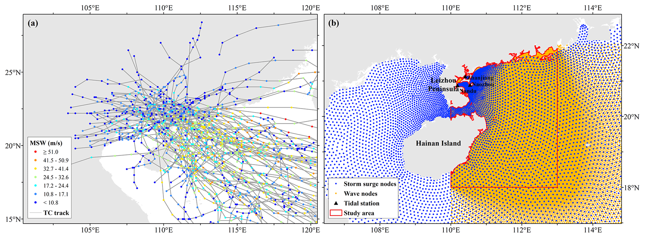
Figure 1Best track and MSW of 86 TCs in this study from 1949 to 2013 (a) and the study area for the joint probability analysis of storm surges and waves of TCs (b).
2.2 Surge heights
The SH dataset is obtained from the Ocean University of China, mainly through the ADvanced CIRCulation model (ADCIRC) simulations, which includes the SHs of 86 TCs affecting the eastern coast of the Leizhou Peninsula and the island of Hainan from 1949 to 2013 (Liu et al., 2018; Li et al., 2016). The previous study provides a water depth map for the study area (Liu et al., 2018). The ADCIRC model integrates the effects of various boundary conditions and external forcing and uses triangular grids with different resolutions, making it more computationally efficient and applicable in numerical simulations. The simulation results are the total water level after the superposition of the water gain caused by a tropical cyclone and astronomical tide, and the time step is 30 min.
To improve the simulation accuracy and computing speed of the hot spot area, the model adopts a triangular grid with nested small- and large-area grids, and the resolutions of different area grids are set in a gradual resolution range from 0.0039 to 0.3∘. The calculation region for the large area is 105.5–121.2∘ E and 3.3–26.4∘ N, and the calculation region for the small area is 105.5–116.5∘ E and 14.7–23.1∘ N (Fig. 2a). And a gradient resolution is used to set the resolution for different regional grids. In the large-area model, the whole large area contains 9331 triangular grid nodes and 18 068 triangles; the resolution of the shoreline in the area near Zhanjiang is 0.07–0.1∘, while the resolution in another area is about 1–2 km. In the small-area model, the whole small area contains 41 153 triangular grid nodes and 79 889 triangles. The resolution of the shoreline near Zhanjiang port is 0.0039–0.01, and the resolution of the open boundary is set to 0.1–0.3∘. The full domain is driven by atmospheric forcing at the surface and surge elevation inversed from the sea surface atmospheric pressure at the open boundary. ADCIRC computes water levels via the solution of the generalized wave continuity equation (GWCE), which is a combined and differentiated form of the continuity and momentum equations:
and the currents are obtained from the vertically integrated momentum equations:
where is total water depth; ζ is the deviation of the water surface from the mean; h is bathymetric depth; is a spherical coordinate conversion factor, and φ0 is a reference latitude; U and V are depth-integrated currents in the x and y directions, respectively; Qλ=UH and Qφ=VH are fluxes per unit width; f is the Coriolis parameter; g is gravitational acceleration; Ps is atmospheric pressure at the surface; ρ0 is the reference density of water; η is the Newtonian equilibrium tidal potential, and α is the effective earth elasticity factor; τs,winds and τs,waves are surface stresses due to winds and waves, respectively; τb is bottom stress; M are lateral stress gradients; D are momentum dispersion terms, and τ0 is a numerical parameter that optimizes the phase propagation properties (Dietrich et al., 2012).
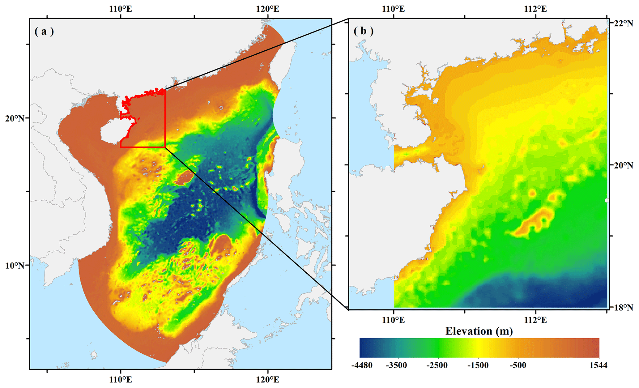
Figure 2The bathymetry of storm surge modeling area (a) and study area (b).
The boundary condition to force the surge in the subdomain is the time series of the water level on each boundary nodes, which includes both the tide elevation of eight major constituents (M2, S2, N2, K2, K1, O1, P1, and Q1) in that area from OSU (Oregon State University) Tidal Prediction Software and the surge elevation extracted from the full domain results (Liu et al., 2018). Comparing the simulation values with the measured surge height at the observation sites, we discover that the absolute standard error is 47 cm, the relative standard error is 22 %, and the simulation results are similar to the observed values in most cases. Thus, the dataset could be used to assess the hazard of TC storm surges. Figure 3a shows an example of the simulation results of the surge height of TC Nasha (ID: 1117) at a specific moment.

Figure 3Distribution of surge height (a) and significant wave height (b) at a specific moment of TC Nasha (ID: 1117) (29 September 2011, 06:00:00 UTC).
2.3 Significant wave heights
The SWH dataset is also obtained from the Ocean University of China, mainly through the Simulating WAves Nearshore (SWAN) model, and includes the SWHs of 86 TC events affecting the study area from 1949 to 2013 (Li et al., 2016). The SWAN model has the advantage of high computational accuracy and stability and has been widely used in numerical simulations of offshore waters. The simulation results include indicators such as significant wave height, mean period, and wave direction, and the time step is 1 h.
The model also uses a triangular grid with nested small- and large-area grids and gradual resolution, but the nodes' scopes and locations differ from those of the storm surge model. The calculation region for the large area is 15–22∘ N, 110.5–118.5∘ E, which has a spatial step of 0.083∘ × 0.083∘; the calculation region for the small area is 21–21.2∘ N, 110–110.5∘ E, which has a spatial step of 0.0033∘ × 0.0033∘ (Fig. 2b). The SWAN model includes land boundaries and water boundaries, which need to be set up separately. The model assumes that the land boundary does not generate waves and assumes that the land boundary can fully absorb waves that cross or leave the shoreline. As the southern and eastern boundaries of the large-area model are open boundaries and are far from the shoreline, which is the focus of this study, the incoming wave energy at the open boundaries of the large-area model can be ignored, and the open boundary conditions for the small area are calculated from the large-area model (Li et al., 2016). The governing equations of the SWAN model are as follows:
The N is wave action density, t is time, λ and φ are geographic space, σ is relative frequency, θ is wave direction, and U and V are the ambient current. cλ, cφ, cθ, and cσ are the propagation velocities in the λ, φ, θ, and σ spaces, respectively. The source term Stot represents wave growth by wind (Dietrich et al., 2012).
Comparing the observed data of buoy stations with the simulated values reveals that the unstructured grid can well reflect the wave variation conditions in the sea. In addition, the mean absolute and root mean square errors of the simulated results of the locally encrypted unstructured triangular grid are the smallest, indicating that the data can effectively reproduce the wave distribution during tropical cyclones. It shall be noted that the effect of sea level rise due to storm surge was not considered during the SWH simulation, which will influence the accuracy of SWHs, especially in intermedia and shallow water. In this paper, we choose the SWH as an indicator of tropical cyclone wave hazard. Figure 3b shows an example of the significant wave height of TC Nasha (ID: 1170) at a specific moment.
2.4 Study area
Based on the location of the nodes of the triangular grid in the storm surge (Sect. 2.2) and wave datasets (Sect. 2.3), we select the region with a dense distribution of both as the study area, and the finalized spatial range is 110–113∘ E, 18–22∘ N (Fig. 1b). This area is located east of the Leizhou Peninsula and the island of Hainan in the South China Sea, which is one of the most frequently affected areas by tropical cyclones in China. Based on the SH and SWH dataset of TCs, we screen 86 historical TC events that simultaneously affected the study area from 1949 to 2013 for joint probability characteristic analysis of storm surge and wave.
Sklar (1973) elucidates the role that copulas play in the relationship between multivariate distribution and their univariate margin distribution and states that any multivariate joint distribution can be described by a univariate marginal distribution function and a couple describing the dependence structure between the variables (Nelsen, 2006). Let F(x) and G(y) be the marginal distributions of x and y, C the copula, and , where H is the bivariate joint distribution function of x and y (Serinaldi, 2015). Therefore, the copula function is widely utilized in multi-hazard joint probability analysis of natural disasters (Chen et al., 2019; Lee et al., 2013).
3.1 Marginal function
The marginal function means that the probability density function (PDF) and cumulative distribution function (CDF) of the univariate are constructed by intensity–frequency analysis to reflect the probability of occurrence of the univariate at different intensities. The method is widely utilized in natural hazard assessments such as tropical cyclones, floods, droughts, and earthquakes. We select five commonly employed marginal functions for the annual extreme fitting of tropical cyclone storm surges and waves, including the Gumbel, Weibull, gamma, exponential, and generalized extreme value (GEV) functions. In this study, the maximum likelihood method is used to estimate the function parameters, based on which the optimal marginal functions for SHs and SWHs are screened by the following steps: firstly, the p value of the K–S test is used to determine whether each node rejects the hypothesis that the samples obey a certain functional distribution. Secondly, the optimal function for each node is screened by three metrics: D value of the K–S test, AIC, and BIC. The smaller the D value of the K–S test, AIC, and BIC, the better the goodness of fit, thus determining the optimal marginal function for each node. Finally, an optimal function is selected as the univariate marginal function for all nodes, and its PDF and CDF are fitted.
3.2 Bivariate copula function
There are a variety of copulas families, including meta-elliptical copulas (normal and t), Archimedean copulas (Clayton, Gumbel, Frank, and Ali–Mikhail–Haq), extreme value (EV) copulas (Gumbel, Husler–Reiss, Galambos, Tawn, and t-EV), and the other families (Plackett and Farlie–Gumbel–Morgenstern) (Chen and Guo, 2019). Among these copulas, the Archimedean copula is more popular for hydrologic applications. The commonly employed Archimedean copula functions include Gumbel, Clayton, and Frank (Table 1), which are selected to analyze the joint probabilities of two variables: the SHs and SWHs of tropical cyclones. Then, the maximum likelihood method is used to estimate the parameters of the copula function. Next, we fit the goodness of fit of copula functions for the tropical cyclone storm surges and waves at each node by the K–S test. According to the passing rate of the K–S test at the sample nodes, an optimal function is selected as the copula function for all nodes of the two-dimensional variables, and the PDF and CDF are calculated.
Table 1Formulas and parameter ranges for three types of bivariate Archimedean copula functions.
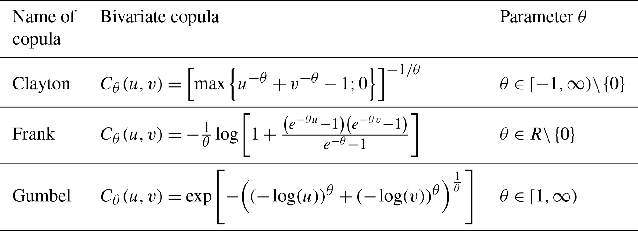
Note: u and v are uniform (0,1) random variables (Nelsen, 2006).
3.3 Joint probability of storm surges and waves
3.3.1 Univariate return period
The return period (RP) indicates the period of natural hazard events, and it is a crucial indicator for quantifying the hazard level, which is widely utilized in hazard analysis. The formula for the return period of a single hazard indicator is as follows:
where RPX is the return period of the univariate X, is the marginal function of the univariate X, and EL denotes the time interval of the sample series of the univariate X. The value is taken as 1 in this paper.
3.3.2 Bivariate probability and return period
Based on the copula function, it can quantitatively estimate the probability of a multivariate being greater than a specified threshold. The bivariate probability refers to the likelihood that various conditions will occur simultaneously, and the bivariate return period refers to the average time interval required for multiple states to be simultaneously greater than a certain threshold.
The definitions of three types of joint probabilities and return periods are given according to the univariate return period formula. The first type is when two variables simultaneously reach a given threshold, which will be defined as the simultaneous probability P∩ (Eq. 6) and simultaneous return period RP∩ (Eq. 7). The second type is that at least one variable reaches a given threshold, which is defined as the joint probability P∪ (Eq. 8) and joint return period RP∪ (Eq. 9). The third type is the conditional probability P| (Eq. 10) and conditional return period RP| (Eq. 11), where when one of the variables reaches a given threshold, the other variable also reaches a certain threshold. The formula is as follows (Serinaldi, 2015):
where FX(x) and FY(y) are the marginal functions of the univariate X and Y, respectively, and is the joint distribution function of the two-dimensional variables (X,Y).
3.3.3 Combined scenario probability
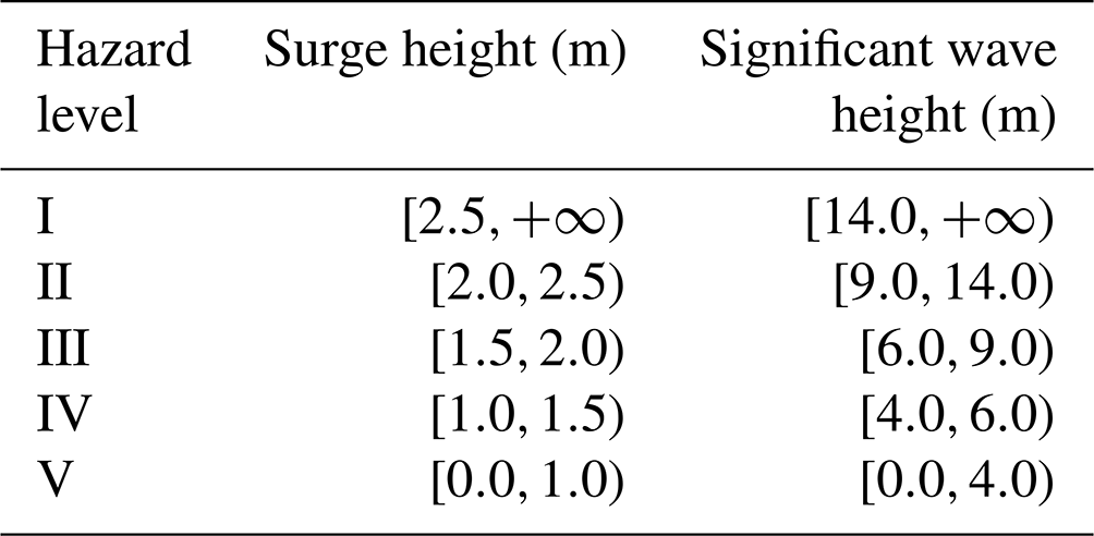
To carry out the tropical cyclone storm surge and wave combination scenario simulation, we classify the SH and SWH into five classes (Table 2) by referring to the “Technical directives for risk assessment and zoning of marine disasters – Part 1: Storm Surge” (MNR, 2019) and “Technical directives for risk assessment and zoning of marine disasters - Part 2: Waves” (MNR, 2021). We calculate the bivariate probabilities for discretized hazard level combination scenarios based on the marginal and copula functions of the storm surge and wave. The formula is as follows:
Table 2Hazard level classification thresholds for combined scenarios of tropical cyclone surge height and significant wave height.
3.4 Design of protection standards for storm surge and wave
3.4.1 Probability changes under increased storm surge and wave protection standards
In actual engineering protection design, if the protection standards of SH and SWH are appropriately increased or decreased, it can change the simultaneous bivariate probability P∩, joint bivariate probability P∪, and conditional bivariate probability P|. In this paper, we try to estimate the change value of the bivariate probability by raising the return period of storm surge or wave. The formula is as follows:
where , , and are the changes of the simultaneous probability P∩, the joint probability P∪, and the conditional probability P| after the univariate return period has been raised; x1 and x2 are the intensity values of variable X for different return periods, respectively, where x2>x1.
3.4.2 Design surge sights and significant wave heights for joint return period scenarios
Based on the binary copula function, the bivariate joint probability of extreme storm surges and waves under different joint return periods is available. In order to achieve the optimal protection effects, it is natural that we need to set the maximum bivariate simultaneous probability of SH and SWH as target functions (Eq. 16) and use joint probability as constraints (Eq. 17).
According to the nonlinear programming method (Bazaraa et al., 2006), for a combined event of extreme SHs and SWHs, a series of (xy) shall be iterated to minimize for a given joint return period to obtain the best cost–benefit effect. Therefore, the optimal values of SH and SWH can be solved, as illustrated in Fig. 4. Since we have the estimation of the joint probability for the study area instead of some specific locations, the optimal design values for SHs and SWHs for all the eastern coasts of the Leizhou Peninsula and the island of Hainan can be estimated.
Figure 4Diagram of determining design surge height and significant wave height based on their joint and simultaneous return periods (red curves are joint return periods (RP∪), black curves are simultaneous return periods (RP∩), and black dots (SHoptimal,SWHoptimal) indicate the optimal design value for SH and SWH).
4.1 Optimal marginal function
Since there are different densities and locations of the triangular grids in the storm surge and wave models, we use the storm surge triangular grid nodes as the benchmark and the wave node closest to each storm surge node as the wave simulation result based on the nearest-neighbor method. Therefore, a dataset of storm surges and waves with the same number and location of nodes is reconstructed, containing 1665 nodes in the study area.
In this paper, based on the reconstructed storm surge and wave simulation results of historical TC events, we calculate each node's annual extremes of SH and SWH. Firstly, the time series of the bivariate annual extremes for all nodes are fitted with five marginal functions, including Gumbel, Weibull, gamma, exponential, and generalized extreme value (GEV). Next, the p value of the K–S test is used to determine whether the hypothesis that the sample obeys a certain theoretical distribution is rejected. Then, we count the number of nodes passing the K–S test for each function and their percentage of all nodes. Finally, the number of nodes and their percentage of each function being selected as optimal is calculated according to the steps for optimal function selection in Sect. 3.1 (Table 3).
Table 3Frequency and percentage of five functions passing the K–S test and the optimal function for all nodes of SH and SWH.
Based on the statistical results, it is found that for fitting the SH, the K–S test of the GEV function had the highest non-rejection rate of 100 %, and the corresponding optimal ratio was 30.04 %, so GEV is set as the optimal marginal function in this study. For the SWH fitting, the number of nodes with no rejection in the K–S test of the GEV function is 1657, accounting for 99.52 % of the total number of nodes, and the corresponding percentage of preferences is also higher than that of other functions. We apply the GEV function to fit the marginal function of the SH and SWH at all nodes and calculate the PDF, CDF, and RP. Figure 5 shows an example of the PDF and CDF of the SH and SWH for a given node.
Figure 5Fitting results of the PDF and CDF of the surge sight and significant wave height based on the GEV function (using node (110.5142∘ E, 20.2768∘ N) as an example).
4.2 Distribution of univariate return periods
Based on the univariate return period formula (Eq. 5), the SH and SWH are estimated for six typical return periods of 5, 10, 20, 50, 100, and 200 years at all nodes. To analyze the distribution characteristics of the univariate return period in this study area, we chose the cubic spline interpolation method to interpolate the intensity values at each node with different return periods into a raster with a resolution of 1 km (Figs. 6 and 7).
Figure 6Spatial distribution of surge heights of tropical cyclones for six typical return periods.
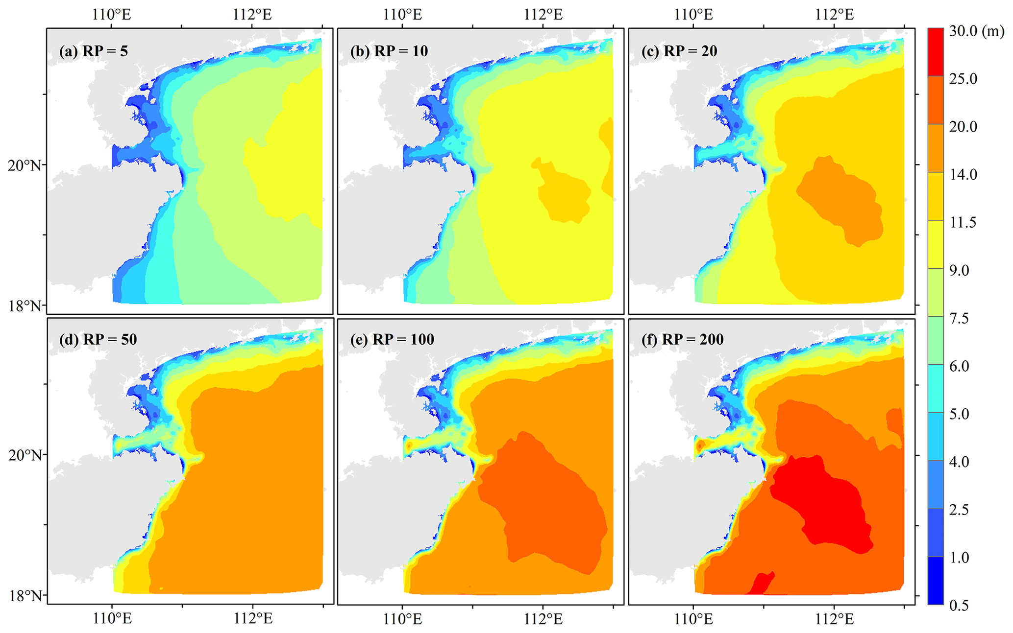
Figure 7Spatial distribution of significant wave heights of tropical cyclones for six typical return periods.
As shown in Fig. 6, the SH shows a significant increasing trend as it approaches the coastline. The SHs along the eastern coast of the Leizhou Peninsula are higher than most other regions. Frequent TC events, TC moving direction (Fig. 1), and pocket-shaped coastal topography (Fig. 2) are all favorable factors to water accumulation in this area. Another area with high SHs is located to the east of the island of Hainan. Besides frequent TCs, this area is at the transition zone from the continental shelf to the continental slope, where bathymetry changes rapidly and can bring strong storm surges easily.
As shown in Fig. 7, the SWHs near the shore are generally smaller than that in the open sea, and there is a significant decreasing trend in SWH as it gets closer to the coastline. This is mainly attributed to the shallow shore depth, island obstruction, wave breaking, and seabed friction attenuation. Among them, the SWHs in the eastern Leizhou Peninsula are lower than that of other seas, which is mainly influenced by the curved depressed coastline and the topography of the shore section. The SWHs are influenced by the frequency, duration, and intensity of TCs, so the SWH is higher in the east and south of the island of Hainan than in the north. The east side of the island of Hainan from the continental shelf to the continental slope causes a wave-breaking effect and dissipation caused by the dramatic change in seafloor topography height, which results in a more significant gradient in SWH. In addition, it shall be noted that errors may be introduced during the estimation of SWHs with GEV due to the limited number of TC events.
4.3 Optimal copula function
The optimal GEV function is utilized as the marginal function for the TC storm surges and waves, based on which three copula functions are applied to the bivariate joint fitting of 1665 nodes. The function parameters are fitted by the maximum likelihood method, and the K–S test is used to determine whether the hypothesis that the sample obeys a certain functional distribution is rejected. Next, we count the number of nodes that pass the K–S test for the three types of copula functions and their percentage of the total number of nodes (Table 4). The statistical results show that the number of nodes passing the K–S test for the Gumbel copula function is 1603, accounting for 96.28 % of all nodes, so it is used as the optimal copula function. The Gumbel copula function is applied to the bivariate joint fitting of SH and SWH for all nodes, and the PDF and CDF are calculated.
Table 4Frequency and percentage of three copula functions passing the K–S test for all nodes of surge height and significant wave height of tropical cyclones.
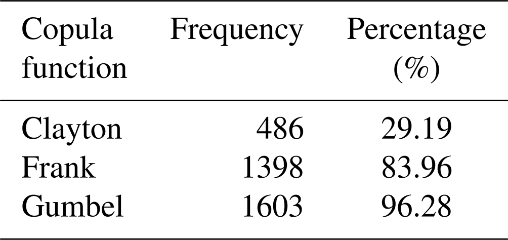
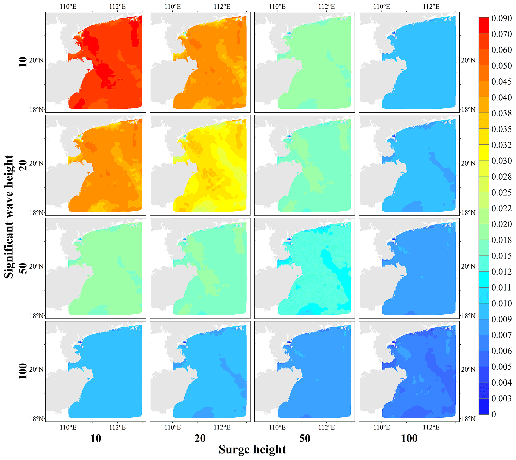
Figure 8Simultaneous probabilities of combined scenarios with four typical return periods for surge height and significant wave heights of tropical cyclones.
4.4 Distribution of bivariate probabilities and return periods
Based on the optimal marginal function and copula function, we calculate RP∩, RP∪, and RP| of SHs and SWHs. In addition, based on the formula of bivariate probability (Eqs. 6 and 8), P∩ and P∪ of SH and SWH are calculated for all nodes with a combination of 10-, 20-, 50-, and 100-year return period scenarios. To analyze the distribution characteristics, P∩ and P∪ for different combinations of return periods at each node are interpolated into a raster with a resolution of 1 km using the cubic spline interpolation method (Figs. 8 and 9).
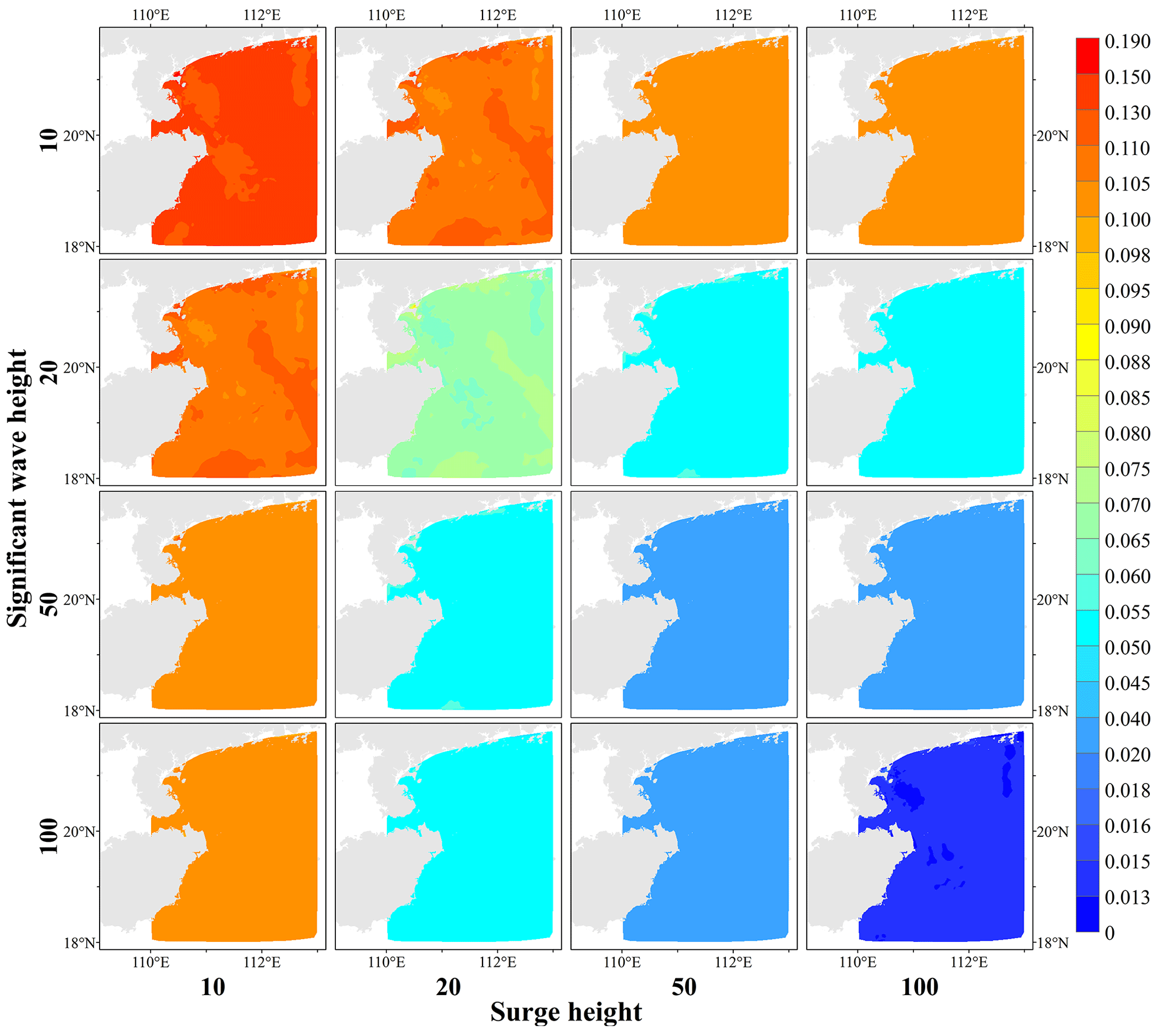
Figure 9Joint probabilities of combined scenarios with four typical return periods for surge height and significant wave heights of tropical cyclones.
The simultaneous bivariate probability P∩ gradually decreases as the return period of SH or SWH increases (Fig. 8). Overall, the closer to the coastline, the higher the P∩ is. P∩ is the greatest when the return period of SH and SWH is 10 years, which is higher than 0.05. P∩ is the smallest for SH and SWH of a 100-year return period, which is generally lower than 0.009.
The joint bivariate probability P∪ of SH and SWH is higher than P∩, and it gradually decreases with an increasing return period of the two hazard indicators (Fig. 9). Overall, the closer to the coastline, the higher the P∪ is. P∪ is the highest when the return period of SH and SWH is 10 years, which is greater than 0.13 overall. P∪ is the smallest when the return period for SH and SWH is 100 years, which is less than 0.015. When the return period of SH or SWH is 50 or 100 years, the regional variations in P∪ are relatively small.
Based on the formula of conditional bivariate probability P| (Eq. 10), we calculate P| for all nodal univariates with different return periods for the other variable in four return periods and interpolate them into 1 km raster data using cubic spline interpolation. According to the formula, the calculation results are consistent when the positions of the variables are swapped. Therefore, only P| for the four return periods of SH in different wave return periods are shown in this paper (Fig. 10). When the SWH is a specific return period, P| gradually decreases as the return period of the SH increases. Under the condition that the return period of SWH is 10 years, P| for SH with a 10-year return period is concentrated between 0.55 and 0.75, and P| is generally less than 0.08 if the return period for SH is 100 years. When the return periods of SWHs and SHs are equivalent, the P| is concentrated between 0.55 and 0.75.
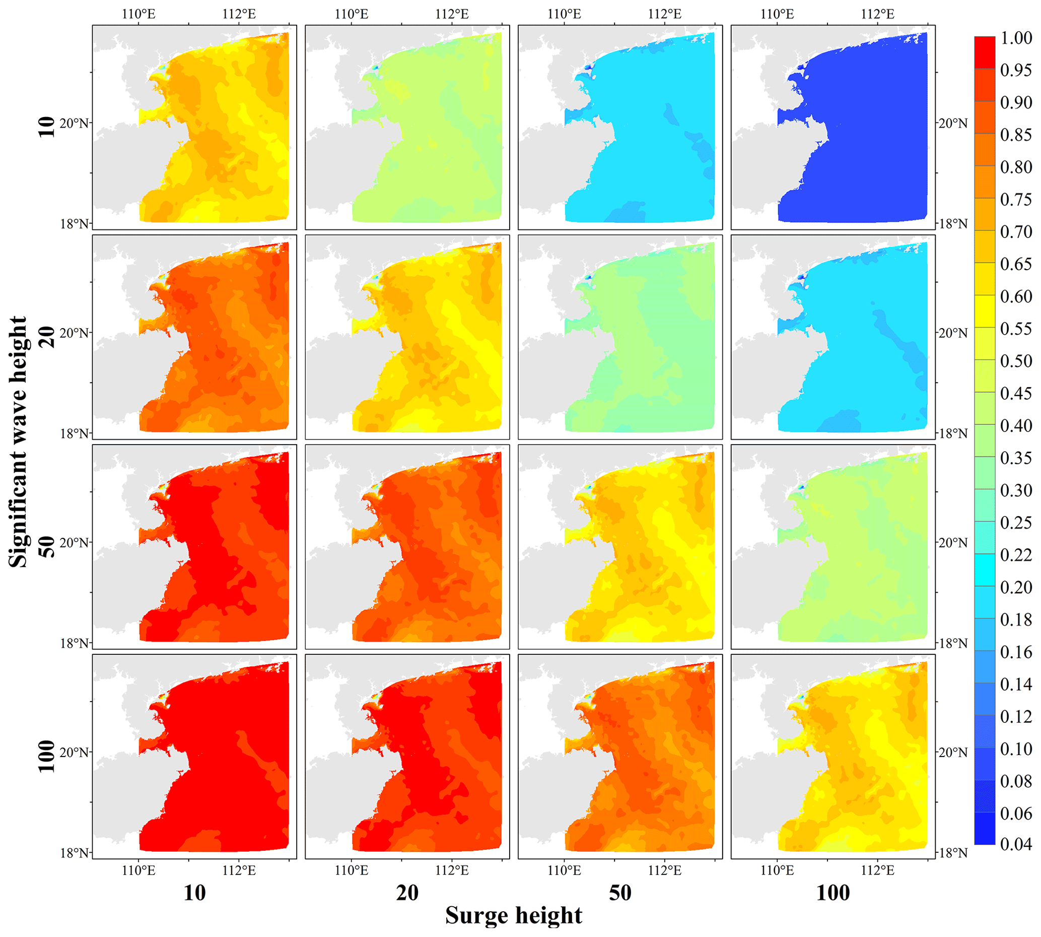
Figure 10Conditional probabilities of bivariate for different return periods of tropical cyclone significant wave heights.
According to the classification thresholds of the hazard indicators (Table 2), SH and SWH are divided into five classes. We calculate the combined scenario probability P& based on Eq. (12) for all nodes with different combinations of SH and SWH for a total of 25 scenarios and interpolate them into 1 km raster data using the cubic spline interpolation method (Fig. 11).
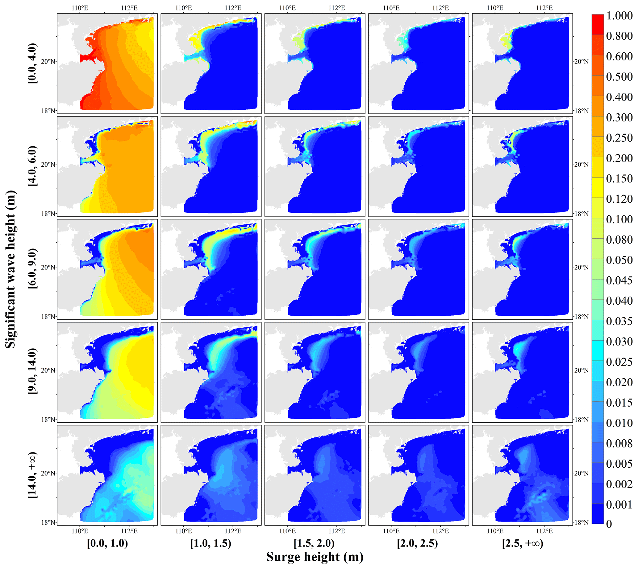
Figure 11Probabilities of combined scenarios with different levels of surge height and significant wave height for tropical cyclones.
Regarding the vertical variation pattern, when the SH hazard level is determined, as the SWH hazard level increases, the high-value area of the combined scenario probability gradually moves away from the coastline, and the scope of the nearshore low-value area gradually expands. This result is consistent with the geographic distribution pattern: the SWH is low nearshore and high offshore. In the horizontal variation pattern, when the hazard level of SWH is determined, as the hazard level of SH increases, the range of low-value areas for the combined scenario probabilities expands, and the low-value area's left boundary gradually approaches the coastline. This result is consistent with the geographic distribution of SHs being high nearshore and low offshore. Overall, the maximum value of the probability for each combined scenario tends to decrease as the hazard level of SH or SWH increases. The larger SH and SWH are concentrated in the eastern Leizhou Peninsula at a certain distance from the coast, with other areas less likely to occur.
Based on the calculated P∩, P∪, P|, and P& with different return periods, Markov chain Monte Carlo (MCMC) and other methods can be further applied to generate random samples for quantitatively assessing TC storm surges and waves. On the other hand, we can explore the effect of varying the intensity values of SH and SWH on the bivariate joint probabilities and apply it to the engineering protection standard.
4.5 Design of protection standards for storm surge and wave
In the design of storm surge and wave protection standards, if one hazard indicator is dominant, upgrading the return period for the other variable can effectively change bivariate P∩ and P∪ when the conditions for their return period protection standard are determined. In this paper, we calculate the change in probability based on Eqs. (13), (14), and (15) to determine the shift in the probability that remains constant when the positions of the two hazard indicators are switched. Therefore, we calculate the change values in P∩, P∪, and P| for all nodes when the return period protection standard for a given variable is increased from 5, 10, 20, and 50 years to 10, 20, 50, and 100 years, respectively. And the data are interpolated into 1 km raster data using the cubic spline interpolation method (Figs. 12, 13, and 14).
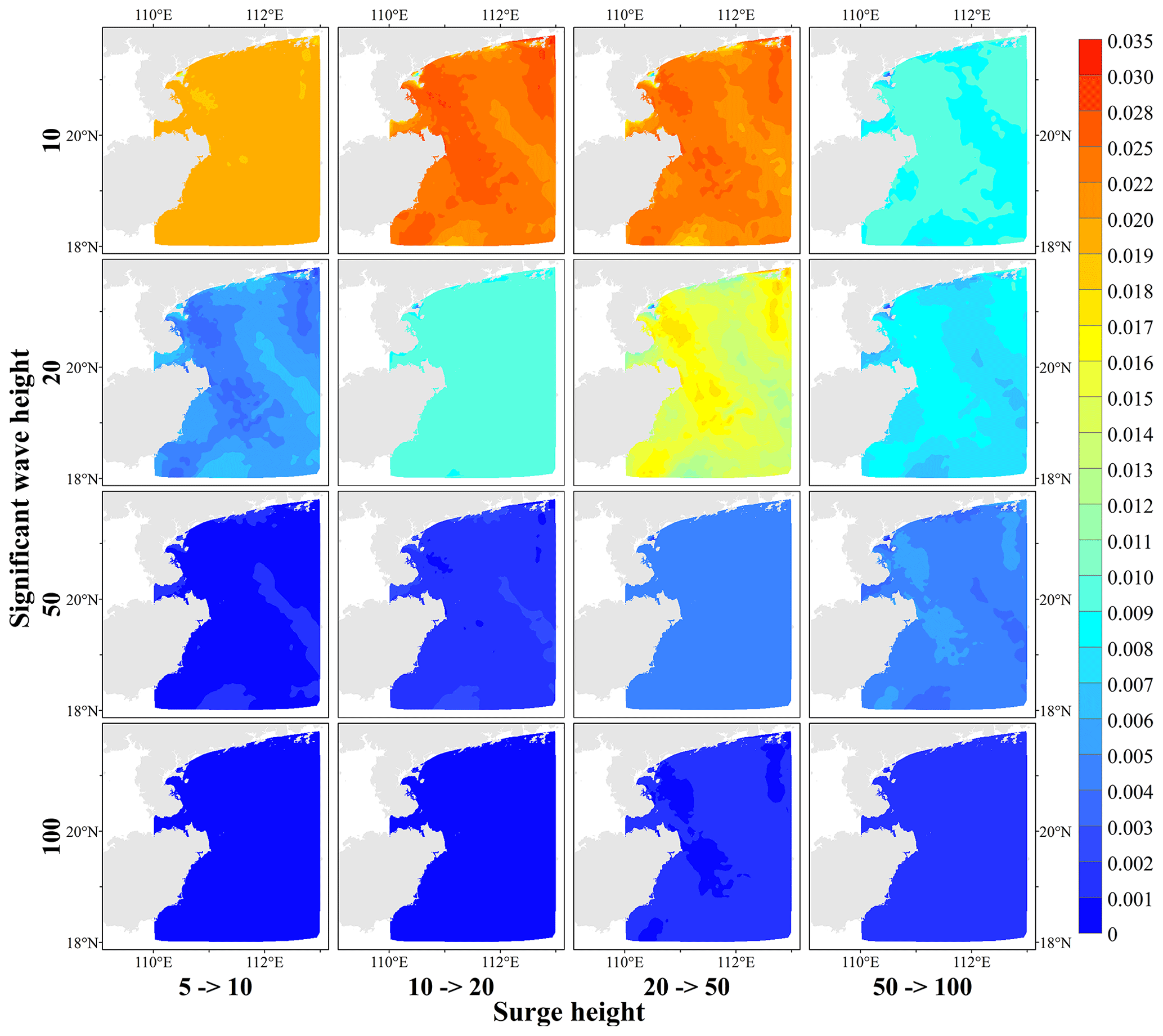
Figure 12Difference in the simultaneous probability of tropical cyclone surge height and significant wave height for scenarios with elevated return period protection standards.
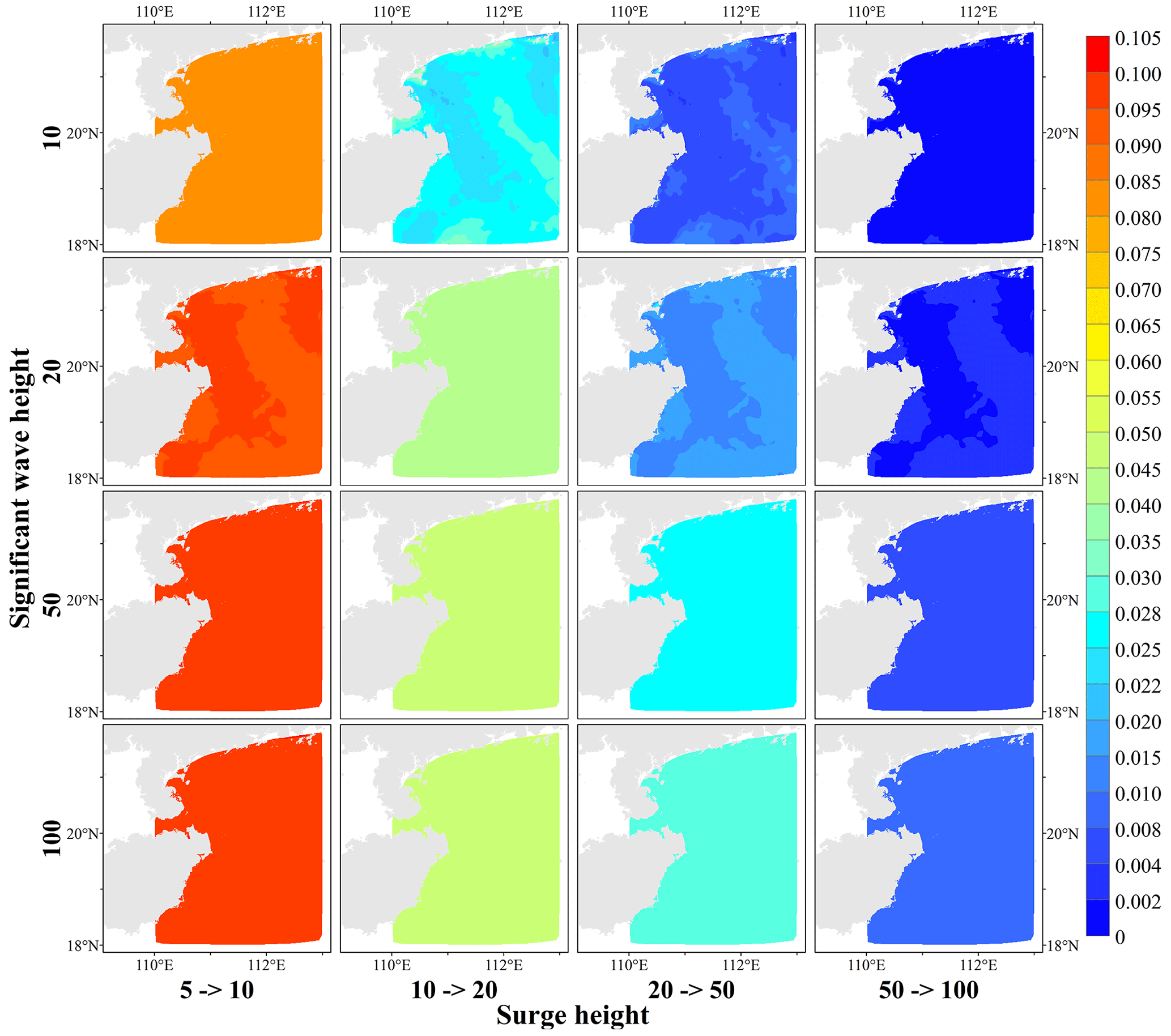
Figure 13Difference in joint probability of tropical cyclone surge height and significant wave height for scenarios with elevated return period protection standards.
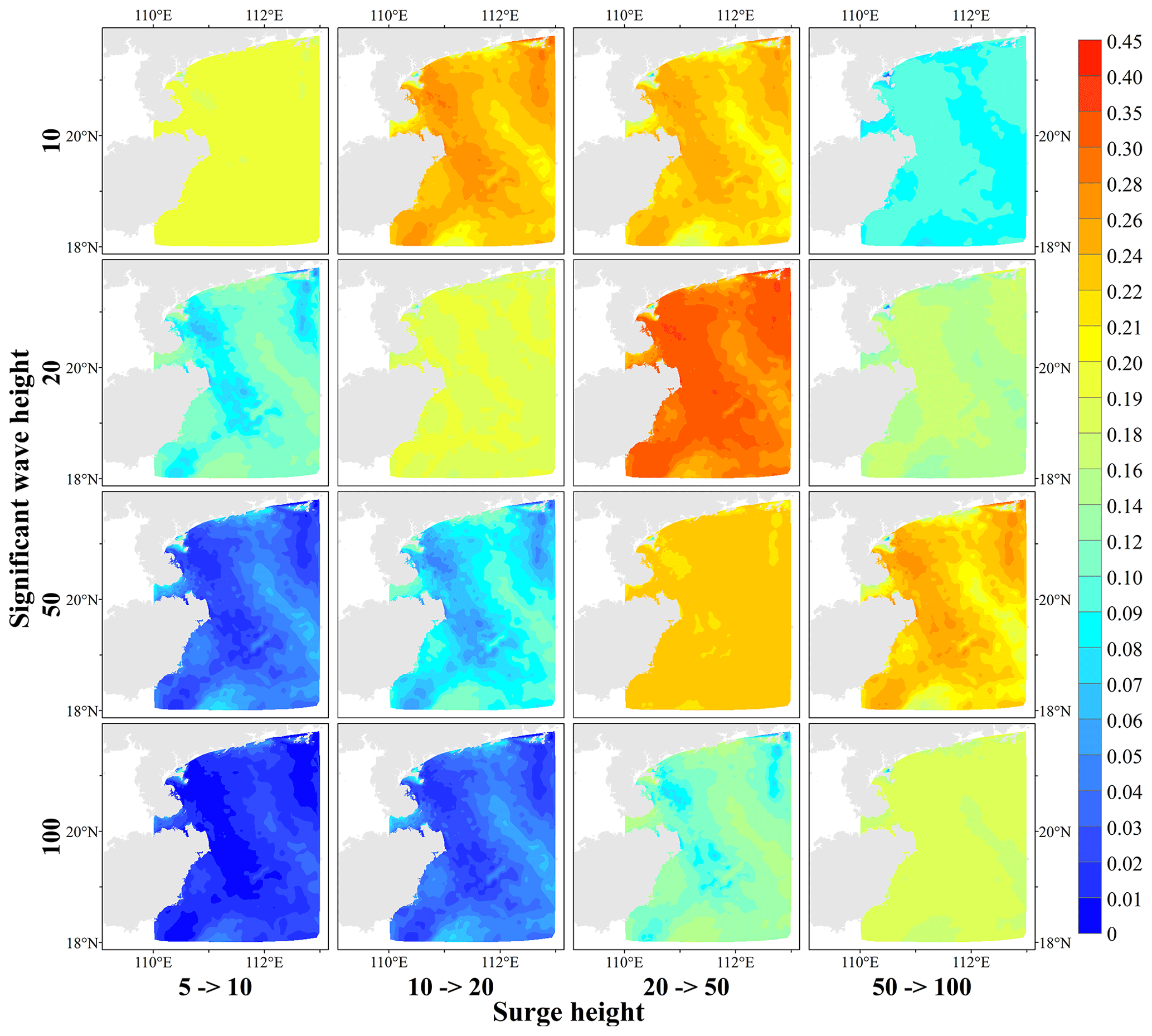
Figure 14Differences in the conditional probability of tropical cyclone surge height and significant wave height for scenarios with elevated return period protection standards.
Figure 12 shows the distribution of the reduction values of bivariate P∩ for the scenario with elevated univariate return period protection standards. As the return period protection standard of one variable increases, the decline in P∩ gradually decreases as the return period protection standard for the other variable increases. Its reduction is concentrated between 0 and 0.035. When the return period protection standard of one variable is fixed, as the design standard of another variable is gradually increased, the decline in P∩ rises to a certain level and then tends to decrease. When the return period of one variable is 10 or 20 years, the decline in P∩ increases when the protection standard of another variable is raised. If the design standard increases from a 50-year to a 100-year return period, the change value of P∩ decreases.
Figure 13 shows the distribution of the reduced values for bivariate P∪ when the protection standard for the univariate return period is increased. Among them, P∪ decreases more than P∩, and the reduced value of P∪ varies from 0 to 0.105. As the return period protection standard for one variable gradually increases, P∪ slowly decreases after the design standard for the other variable has increased. When the return period protection standard for one variable is fixed, the decline in P∪ gradually decreases as the design standard for the other variable is increased.
Figure 14 shows the distribution of the reduced values of bivariate P| for the scenario of raising the univariate return period protection standard. As the return period for one variable increases, the decreasing value of P| tended to decrease after increasing the design standard for the other variable. P| has a more significant decrease than P∩ and P∪, and the decreasing value of P| varies from 0 to 0.45. When the protection standard of one variable is fixed and low, the reduction in P| will tend to decrease after the design standard of another variable has been raised to a certain level. When the protection standard for one variable is a 10- or 20-year return period, the decrease in bivariate P| tends to increase when the design standard for the other variable's return period is raised, but the decrease in P| is slightly reduced when the design standard of the other variable is increased from a 50-year to a 100-year return period. If the protection standard of one variable is high, the decrease in P| after the design standard of the other variable has been raised always tends to increase.
In the engineering protection standard, the appropriate design values of the SHs and SWHs are set according to the bivariate RP∪ and RP∩, and the estimation method is shown in Sect. 3.4.2. In this paper, the design values of SH and SWH for six RP∪ for all nodes are calculated based on the above method and interpolated to 1 km raster data by the cubic spline interpolation method (Figs. 15 and 16). The design SH and SWH show an apparent increasing trend as the return period increases, with the high-value area for SH constantly concentrated east of the Leizhou Peninsula and the high-value area for SWH concentrated in the east of the island of Hainan.
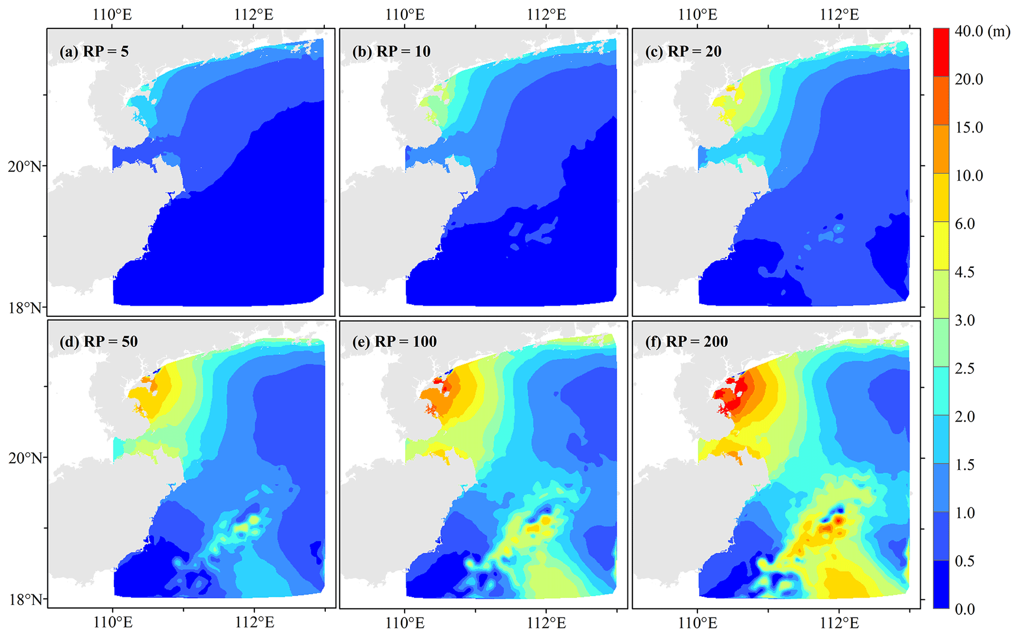
Figure 15Design surge heights for six typical joint return period scenarios.
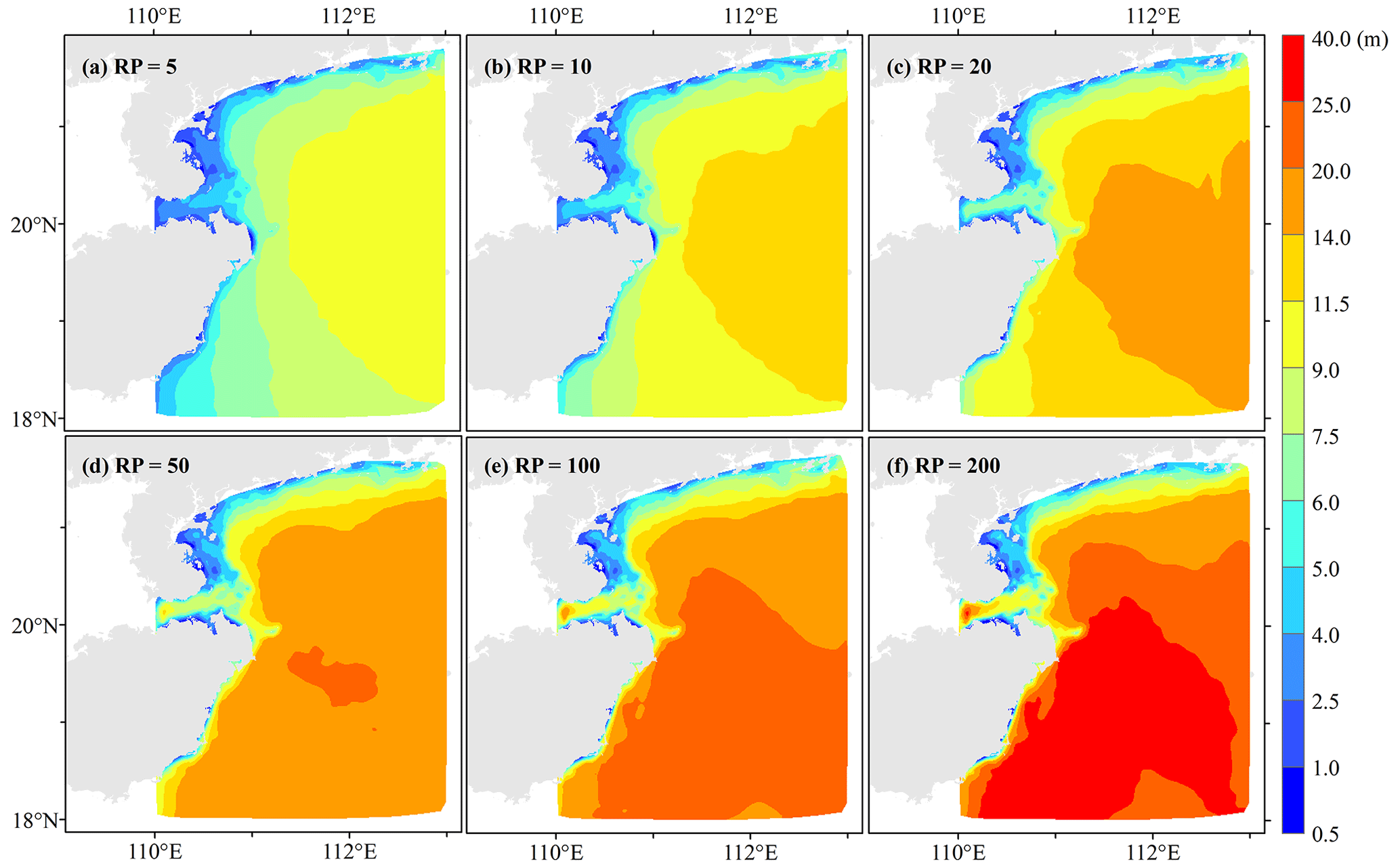
Figure 16Design significant wave heights for six typical joint return period scenarios.
When RP∪ is a 5-year return period, the design SHs are between 1.5 and 2.5 m in the eastern coastal area of the Leizhou Peninsula and fall below 0.5 m in the southeastern coastal region of the island of Hainan. As the return period increases, the design SH gradually increases, and when RP∪ is a 200-year return period, the design SH in the eastern coastal area of the Leizhou Peninsula is generally higher than 3.0 m. The design SH in the northeast coastal area of the island of Hainan is mainly between 3.0 and 15.0 m, while that in the southeast coastal region of the island of Hainan is between 0.5 and 2.0 m, which is lower than that in the northeast.
When RP∪ is a 5-year return period, the design SWHs in the coastal areas of the Leizhou Peninsula and the island of Hainan are less than 2.5 m overall. Further away from the coastline, the design SWH gradually increases. As the return period increases, the design SWH gradually increases, and the growth is more evident than that of SH. When RP∪ is a 200-year return period, the design SWH along the coast of the Leizhou Peninsula is generally less than 6.0 m, while the design SWH along the Qiongzhou Strait and southeastern the island of Hainan is relatively high.
In this study, we aimed to estimate joint probability analysis of storm surges and waves using copula functions on a large dataset from a wide area and to determine their respective design standards as scalar values of SWH and SH. Our main conclusions are as follows:
-
The GEV function is the most suitable for fitting the probability distribution characteristics of the annual extremes of tropical cyclone SH and SWH for all nodes in the study area. The Gumbel copula function is appropriate as a bivariate joint distribution function for all nodes in the study area.
-
The hazard of a single indicator can be characterized by the univariate intensity values with different return periods, which the optimal marginal function can estimate. Our findings show that the SH exhibits a significant increasing trend closer to the coastline, while SWH is higher farther from the shoreline across different return periods. However, we also observe apparent spatial heterogeneity in the distribution, influenced by factors such as the shoreline shape, coastal and submarine topography, and deflection forces.
-
Bivariate probabilities are utilized in this study to assess the integrated hazard of multiple indicators, including P∩, P∪, P|, and P&, which effectively compensates for the deficiency of disregarding the correlation among variables in univariate hazard assessment. These four probabilities can visually describe the occurrence probability for different combinations of scenarios; the more significant the probability is, the higher the hazard. Overall, P| is the largest, P∪ is the second largest, and P∩ is the smallest, while P& is influenced by the classification of single hazard indicators. When one variable is constant, P∩, P∪, and P| tend to decrease as the return period of the other variable increases.
-
In the actual design for engineering protection standards, the bivariate P∩, P∪, and P| can be reduced by appropriately increasing the design values of the SHs and SWHs. When the return period protection standard of one variable is fixed, as the design standards of another variable gradually increase, the decline in P∩ and P| rises to a certain level and then tends to decrease, but the decline in P∪ gradually decreases. Therefore, developing appropriate design standards for the SHs and SWHs can effectively reduce the impact of tropical cyclone marine hazards on coastal areas. Since the joint probability distribution of the bivariate is a three-dimensional surface, to obtain specific scalar values for these two hazards as design standards, in this study, the optimal design SHs and SWHs under the objective of minimum bivariate simultaneous return period are estimated using a nonlinear programming approach with their estimated joint return periods as constraints.
Although this study provides helpful insights into joint probability analysis of storm surges and waves using copula functions, several limitations need to be addressed in future research. One limitation is the absence of water level rise caused by storm surges in the numerical modeling of waves, which may introduce errors in the simulation of SWHs in intermediate and shallow water. In addition, exploring the contribution of other indicators, such as long-term sea level rise as environmental hazards, can further improve the accuracy of hazard assessment.
We have used R programming language for joint probability analysis, and the code is available at https://doi.org/10.5281/zenodo.8172520 (Fang et al., 2023).
The datasets used in this study are available at https://tcdata.typhoon.org.cn/zjljsjj_zlhq.html (Lu et al., 2021).
FWH and ZHX conceived the research framework and developed the methodology. ZHX was responsible for the code compilation, data analysis, graphic visualization, and first draft writing. FWH managed the implementation of research activities and revised the manuscript. CM participated in the data collection of this study. All authors discussed the results and contributed to the final version of the paper.
The contact author has declared that none of the authors has any competing interests.
Publisher’s note: Copernicus Publications remains neutral with regard to jurisdictional claims in published maps and institutional affiliations.
The authors acknowledge the financial support of the National Key Research and Development Program of China and the Key Special Project for Introduced Talents Team of Southern Marine Science and Engineering Guangdong Laboratory (Guangzhou). We are grateful to Xing Liu of the Ocean University of China for providing the simulation data of storm surges and waves for historical tropical cyclone events.
This research has been supported by the National Key Research and Development Program of China (grant nos. 2017YFA0604903 and 2018YFC1508803) and the Key Special Project for Introduced Talents Team of the Southern Marine Science and Engineering Guangdong Laboratory (Guangzhou) (grant no. GML2019ZD0601).
This paper was edited by Brunella Bonaccorso and reviewed by Francesco Serinaldi and two anonymous referees.
Bazaraa, M. S., Sherali, H. D., and Shetty, C. M.: Nonlinear programming: Theory and algorithms, 3rd edn., John Wiley & Sons, Hoboken, New Jersey, 872 pp., ISBN 978-0-471-48600-8, 2006.
Bilskie, M. V., Hagen, S. C., Medeiros, S. C., Cox, A. T., Salisbury, M., and Coggin, D.: Data and numerical analysis of astronomic tides, wind-waves, and hurricane storm surge along the northern Gulf of Mexico, J. Geophys. Res.-Oceans, 121, 3625–3658, https://doi.org/10.1002/2015JC011400, 2016.
Bomers, A., Schielen, R. M. J., and Hulscher, S. J. M. H.: Consequences of dike breaches and dike overflow in a bifurcating river system, Nat. Hazards, 97, 309–334, https://doi.org/10.1007/s11069-019-03643-y, 2019.
Brown, J. M.: A case study of combined wave and water levels under storm conditions using WAM and SWAN in a shallow water application, Ocean Model., 35, 215–229, https://doi.org/10.1016/j.ocemod.2010.07.009, 2010.
Cavanaugh, J. E. and Neath, A. A.: The Akaike information criterion: Background, derivation, properties, application, interpretation, and refinements, WIREs Comp. Stat., 11, e1460, https://doi.org/10.1002/wics.1460, 2019.
Chen, L. and Guo, S.: Copulas and its application in hydrology and water resources, 1st edn., Springer, Singapore, 290 pp., https://doi.org/10.1007/978-981-13-0574-0, 2019.
Chen, Y. and Yu, X.: Sensitivity of storm wave modeling to wind stress evaluation methods, J. Adv. Model. Earth Sy., 9, 893–907, https://doi.org/10.1002/2016MS000850, 2017.
Chen, Y., Li, J., Pan, S., Gan, M., Pan, Y., Xie, D., and Clee, S.: Joint probability analysis of extreme wave heights and surges along China's coasts, Ocean Eng., 177, 97–107, https://doi.org/10.1016/j.oceaneng.2018.12.010, 2019.
Corbella, S. and Stretch, D. D.: Simulating a multivariate sea storm using Archimedean copulas, Coast. Eng., 76, 68–78, https://doi.org/10.1016/j.coastaleng.2013.01.011, 2013.
Dietrich, J. C., Tanaka, S., Westerink, J. J., Dawson, C. N., Luettich, R. A., Zijlema, M., Holthuijsen, L. H., Smith, J. M., Westerink, L. G., and Westerink, H. J.: Performance of the unstructured-mesh, SWAN+ADCIRC model in computing hurricane waves and surge, J. Sci. Comput., 52, 468–497, https://doi.org/10.1007/s10915-011-9555-6, 2012.
Fang, W., Zhang, H., and Cheng, M.: Code for joint probabilistic analysis of storm surges and waves (Version v1.0), Zenodo [code], https://doi.org/10.5281/zenodo.8172520, 2023.
Galiatsatou, P. and Prinos, P.: Joint probability analysis of extreme wave heights and storm surges in the Aegean Sea in a changing climate, E3S Web Conf., 7, 02002, https://doi.org/10.1051/e3sconf/20160702002, 2016.
Hsu, C. H., Olivera, F., and Irish, J. L.: A hurricane surge risk assessment framework using the joint probability method and surge response functions, Nat. Hazards, 91, 7–28, https://doi.org/10.1007/s11069-017-3108-8, 2018.
Huang, Y., Weisberg, R. H., Zheng, L., and Zijlema, M.: Gulf of Mexico hurricane wave simulations using SWAN: Bulk formula-based drag coefficient sensitivity for Hurricane Ike, J. Geophys. Res.-Oceans, 118, 3916–3938, https://doi.org/10.1002/jgrc.20283, 2013.
Hughes, S. A. and Nadal, N. C.: Laboratory study of combined wave overtopping and storm surge overflow of a levee, Coast. Eng., 56, 244–259, https://doi.org/10.1016/j.coastaleng.2008.09.005, 2009.
Jang, J. H. and Chang, T. H.: Flood risk estimation under the compound influence of rainfall and tide, J. Hydrol., 606, 127446, https://doi.org/10.1016/j.jhydrol.2022.127446, 2022.
Kimf, K. O., Yuk, J., Leen, H. S., and Choi, B. H.: Typhoon Morakot induced waves and surges with an integrally coupled tide-surge-wave finite element model, J. Coastal Res., 2, 1122–1126, https://doi.org/10.2112/SI75-225.1, 2016.
Lee, D. Y. and Jun, K. C.: Estimation of design wave height for the waters around the Korean Peninsula, Ocean Sci. J., 41, 245–254, https://doi.org/10.1007/BF03020628, 2006.
Lee, T., Modarres, R., and Ouarda, T. B. M. J.: Data-based analysis of bivariate copula tail dependence for drought duration and severity, Hydrol. Process., 27, 1454–1463, https://doi.org/10.1002/hyp.9233, 2013.
Li, J., Fang, W., Zhang, X., Cao, S., Yang, X., Liu, X., and Sun, J.: Similar tropical cyclone retrieval method for rapid potential storm surge and wave disaster loss assessment based on multiple hazard indictors, Mar. Sci., 40, 49–60, https://doi.org/10.11759/hykx20151104001, 2016.
Li, L., Pan, Y., Amini, F., and Kuang, C.: Full scale study of combined wave and surge overtopping of a levee with RCC strengthening system, Ocean Eng., 54, 70–86, https://doi.org/10.1016/j.oceaneng.2012.07.021, 2012.
Lin, N., Emanuel, K. A., Smith, J. A., and Vanmarcke, E.: Risk assessment of hurricane storm surge for New York City, J. Geophys. Res.-Atmos., 115, D18121, https://doi.org/10.1029/2009JD013630, 2010.
Liu, X., Jiang, W., Yang, B., and Baugh, J.: Numerical study on factors influencing typhoon-induced storm surge distribution in Zhanjiang Harbor, Estuar. Coast. Shelf S., 215, 39–51, https://doi.org/10.1016/j.ecss.2018.09.019, 2018.
Lu, X., Yu, H., Ying, M., Zhao, B., Zhang, S., Lin, L., Bai, L., and Wan, R.: Western North Pacific tropical cyclone database created by the China Meteorological Administration, Adv. Atmos. Sci., 38, 690–699, https://doi.org/10.1007/s00376-020-0211-7, 2021 (data available at: https://tcdata.typhoon.org.cn/zjljsjj_zlhq.html, last access: 18 July 2023).
Marcos, M., Rohmer, J., Vousdoukas, M. I., Mentaschi, L., Le Cozannet, G., and Amores, A.: Increased extreme coastal water levels due to the combined action of storm surges and wind waves, Geophys. Res. Lett., 46, 4356–4364, https://doi.org/10.1029/2019GL082599, 2019.
MNR: Technical directives for risk assessment and zoning of marine disaster – Part 1: Storm surge, Ministry of Natural Resources of the People's Republic of China, https://www.renrendoc.com/p-82139795.html (last access: 18 July 2023), 2019.
MNR: Technical directives for risk assessment and zoning of marine disaster – Part 2: Wave, Ministry of Natural Resources of the People's Republic of China, https://www.doc88.com/p-70187168096035.html (last access: 18 July 2023), 2021.
Morellato, D. and Benoit, M.: Constitution of a numerical wave data-base along the French Mediterranean coasts through hindcast simulations over 1979-2008, Rev. Paralia, 3, 13–24, https://doi.org/10.5150/revue-paralia.2010.005, 2010.
Muraleedharan, G., Rao, A. D., Kurup, P. G., Nair, N. U., and Sinha, M.: Modified Weibull distribution for maximum and significant wave height simulation and prediction, Coast. Eng., 54, 630–638, https://doi.org/10.1016/j.coastaleng.2007.05.001, 2007.
Neath, A. A. and Cavanaugh, J. E.: The Bayesian information criterion: Background, derivation, and applications, WIREs Comp. Stat., 4, 199–203, https://doi.org/10.1002/wics.199, 2012.
Nelsen, R. B.: An intruduction to copulas, 2nd edn., Springer, New York, 269 pp., https://doi.org/10.1007/0-387-28678-0, 2006.
Niedoroda, A. W., Resio, D. T., Toro, G. R., Divoky, D., Das, H. S., and Reed, C. W.: Analysis of the coastal Mississippi storm surge hazard, Ocean Eng., 37, 82–90, https://doi.org/10.1016/j.oceaneng.2009.08.019, 2010.
Pan, Y., Li, L., Amini, F., and Kuang, C.: Full-scale HPTRM-strengthened levee testing under combined wave and surge overtopping conditions: Overtopping hydraulics, shear stress, and erosion analysis, J. Coastal Res., 29, 182–200, https://doi.org/10.2112/JCOASTRES-D-12-00010.1, 2013.
Pan, Y., Zhang, Z., Yuan, S., Zhou, Z., and Chen, Y.: An overview of research on combined wave and surge overtopping on levees, Adv. Sci. Technol. Water Resour., 39, 90–94, https://jour.hhu.edu.cn/slsdkjjz/article/pdf/jz20190115 (last access: 18 July 2023), 2019.
Papadimitriou, A. G., Chondros, M. K., Metallinos, A. S., Memos, C. D., and Tsoukala, V. K.: Simulating wave transmission in the lee of a breakwater in spectral models due to overtopping, Appl. Math. Model., 88, 743–757, https://doi.org/10.1016/j.apm.2020.06.061, 2020.
Perk, L., Rijn, L. van, Koudstaal, K., and Fordeyn, J.: A rational method for the design of sand dike/dune systems at sheltered sites; Wadden Sea Coast of Texel, The Netherlands, J. Mar. Sci. Eng., 7, 324, https://doi.org/10.3390/jmse7090324, 2019.
Petroliagkis, T. I., Voukouvalas, E., Disperati, J., and Bidlot, J.: Joint probabilities of storm surge, significant wave height and river discharge components of coastal flooding events, JRC Technical Report EUR 27824 EN, 79 pp., https://doi.org/10.2788/677778, 2016.
Rao, X., Li, L., Amini, F., and Tang, H.: Numerical study of combined wave and surge overtopping over RCC strengthened levee systems using the smoothed particle hydrodynamics method, Ocean Eng., 54, 101–109, https://doi.org/10.1016/j.oceaneng.2012.06.024, 2012.
Serinaldi, F.: Dismissing return periods!, Stoch. Env. Res. Risk A., 29, 1179–1189, https://doi.org/10.1007/s00477-014-0916-1, 2015.
Shi, X., Han, Z., Fang, J., Tan, J., Guo, Z., and Sun, Z.: Assessment and zonation of storm surge hazards in the coastal areas of China, Nat. Hazards, 100, 39–48, https://doi.org/10.1007/s11069-019-03793-z, 2020.
Sklar, A.: Random variables, joint distribution functions, and copulas, Kybernetika, 9, 449–460, https://www.kybernetika.cz/content/1973/6/449/paper.pdf (last access: 18 July 2023), 1973.
Teena, N. V., Sanil Kumar, V., Sudheesh, K., and Sajeev, R.: Statistical analysis on extreme wave height, Nat. Hazards, 64, 223–236, https://doi.org/10.1007/s11069-012-0229-y, 2012.
Trepanier, J. C., Needham, H. F., Elsner, J. B., and Jagger, T. H.: Combining surge and wind risk from hurricanes using a copula model: An example from Galveston, Texas, Prof. Geogr., 67, 52–61, https://doi.org/10.1080/00330124.2013.866437, 2015.
Wahl, T., Mudersbach, C., and Jensen, J.: Assessing the hydrodynamic boundary conditions for risk analyses in coastal areas: a multivariate statistical approach based on Copula functions, Nat. Hazards Earth Syst. Sci., 12, 495–510, https://doi.org/10.5194/nhess-12-495-2012, 2012.
Wahl, T., Jain, S., Bender, J., Meyers, S. D., and Luther, M. E.: Increasing risk of compound flooding from storm surge and rainfall for major US cities, Nat. Clim. Change, 5, 1093–1097, https://doi.org/10.1038/nclimate2736, 2015.
Xie, D., Zou, Q., and Cannon, J. W.: Application of SWAN+ADCIRC to tide-surge and wave simulation in Gulf of Maine during Patriot’s Day storm, Water Sci. Eng., 9, 33–41, https://doi.org/10.1016/j.wse.2016.02.003, 2016.
Xu, H., Tan, J., Li, M., and Wang, J.: Compound flood risk of rainfall and storm surge in coastal cities as assessed by copula formal, J. Nat. Disasters, 31, 40–48, https://doi.org/10.13577/j.jnd.2022.0104, 2022.
Zhang, B. and Wang, S.: Probabilistic characterization of extreme storm surges induced by tropical cyclones, J. Geophys. Res.-Atmos., 126, e2020JD033557, https://doi.org/10.1029/2020JD033557, 2021.