Accounting for path and site effects in spatial ground-motion correlation models using Bayesian inference

Ground-motion correlation models play a crucial role in regional seismic risk modeling of spatially distributed built infrastructure. Such models predict the correlation between ground-motion amplitudes at pairs of sites, typically as a function of their spatial proximity. Data from physics-based simulators and event-to-event variability in empirically derived model parameters suggest that spatial correlation is additionally affected by path and site effects. Yet, identifying these effects has been difficult due to scarce data and a lack of modeling and assessment approaches to consider more complex correlation predictions. To address this gap, we propose a novel correlation model that accounts for path and site effects via a modified functional form. To quantify the estimation uncertainty, we perform Bayesian inference for model parameter estimation. The derived model outperforms traditional isotropic models in terms of the predictive accuracy for training and testing data sets. We show that the previously found event-to-event variability in model parameters may be explained by the lack of accounting for path and site effects. Finally, we examine implications of the newly proposed model for regional seismic risk simulations.

1 Introduction

Earthquakes can cause widespread damage to the built environment, exposing its users to severe and potentially long-lasting societal stress. Analyzing earthquake-induced consequences is key to enhancing efficient and targeted seismic risk management strategies. Empirical ground-motion models (GMMs) are widely used for the prediction of earthquake-induced ground-motion intensity measures (IMs) at individual sites. The assessment of consequences to spatially distributed systems, such as the residential building stock of an urban area or its road network, additionally requires spatial correlation models to characterize the dependency among IMs at different sites (Wesson and Perkins, 2001; Lee and Kiremidjian, 2007).

A predictive spatial correlation model consists of a functional form, one or several dependent variables, and the model parameters. Early studies, such as Boore et al. (2003), as well as more recent studies, such as Schiappapietra and Douglas (2020), use an isotropic model where the correlation among sites decays exponentially (the functional form) with increasing Euclidean distance between sites (the dependent variable). Observations of pairs of IMs from past earthquakes are used to calibrate these models. The isotropic assumption allows grouping of station pairs with similar distance for the estimation of model parameters via geo-statistical curve-fitting techniques.

To alleviate the scarcity of data, some researchers pooled data from multiple earthquakes and assumed that the same correlation model parameters apply to different events (e.g., Goda and Atkinson, 2010; Esposito and Iervolino, 2011). Other studies estimated separate models for individual earthquakes and reported that the corresponding parameters vary from one earthquake to another (e.g., Jayaram and Baker, 2009; Goda, 2011). Sokolov et al. (2012) mention that this event-to-event variability may be caused by site effects (i.e., stronger correlation amongst sites with similar geological conditions) and path effects (i.e., stronger correlation amongst sites with similar wave propagation paths). While the importance of site and path effects became apparent in data from physics-based ground-motion simulators (Chen and Baker, 2019), the findings with respect to recorded ground-motion data differ amongst previous studies. Early work of Jayaram and Baker (2009) and Sokolov et al. (2012) found that, for example, the heterogeneity of soil conditions may influence spatial correlations. Yet, more recent studies could not find such evidence and suggested accounting for event-to-event variability via random variables for model parameters in regional seismic risk analyses (Heresi and Miranda, 2019) or deriving region-specific correlation models (Schiappapietra and Douglas, 2020).

Identifying explanatory factors by estimating correlation models from data of individual earthquakes is challenging. First, the comparison of a single model parameter estimate per event with a single metric describing a certain aspect of the region the event was recorded in (such as the heterogeneity of soil conditions) suffers from scarcity of data. Estimation of event-specific correlation model parameters requires data from particularly well-recorded events, of which there are only a few. Second, the use of an isotropic model and the condensation to a single parameter estimate per event may hide path and site effects that are present within the event data. Third, the estimated model parameters are subject to varying degrees of estimation uncertainty because the underlying data sets stem from earthquakes that were recorded by a different number and layout of seismic network stations. Schiappapietra and Douglas (2021) and Baker and Chen (2020) aimed to quantify this uncertainty via simulating data from an assumed “true” model and comparing the latter to the model estimated from the simulated data using different estimation techniques. Both studies, however, used the same isotropic model with an exponential functional form that has only one model parameter, and Baker and Chen (2020) reported difficulties in extending the proposed method to models with more than one parameter.

This study explores novel correlation models that, in addition to spatial proximity, also account for path and site effects. In contrast to previous studies, we do so by modifying and extending the functional form and the dependent variables of the correlation models. The increased complexity of these models calls for a consistent quantification of the inherent estimation uncertainty, thus complicating the use of conventional geo-statistical curve-fitting techniques. To address this, we use Bayesian inference to estimate the model parameters. While Bayesian inference has been proposed for GMMs in the past (e.g., Moss and Der Kiureghian, 2006; Stafford, 2019), it has not been applied to study spatial ground-motion correlation.

We present the proposed correlation model in Sect. 2. Section 3 introduces the Bayesian inference scheme used to estimate the model parameters from the PEER NGA-West2 data set (Ancheta et al., 2014). Using the same data set, Sect. 4 first compares the proposed correlation models to event-specific isotropic models by employing a novel metric to quantify the predictive accuracy and then compares model performance on test data from the 2019 Ridgecrest, California, earthquake sequence (Rekoske et al., 2020). Finally, Sect. 5 examines implications of the novel correlation model for regional seismic risk simulation studies.

2 Spatial correlation models for ground-motion amplitudes

This study on spatial correlation models builds on empirically derived GMMs that predict a ground-motion IM at site i induced by an earthquake rupture k as

$$\begin{array}{}\text{(1)}& \ln {\mathrm{IM}}_{ki}={\mathit{\mu }}_{\ln \mathrm{IM}}({\mathrm{rup}}_k,{\mathrm{site}}_i)+\mathit{\delta }{B}_k+\mathit{\delta }{W}_{ki},\end{array}$$

where μ_ln IM(⋅) is the predicted mean ln IM value as a function of rupture (rup) and site (site) characteristics (Baker et al., 2021). Amongst others, these typically include earthquake magnitude, rupture mechanism, source-to-site distance, and site-specific geological information. The between-event and within-event residuals, δB_k and δW_ki, are assumed to be independent, normally distributed variables with standard deviations τ and ϕ, respectively. Empirical GMMs provide the mean function μ_ln IM(⋅), as well as the standard deviations τ and ϕ. For a specific event, the between-event residual denotes a common deviation from the predicted mean that is constant for all sites, whereas the within-event residuals vary in space. For this correlation study, we scale the within-event residual by its standard deviation ϕ and denote the scaled within-event residual as $Z_{ki}=\mathit{\delta }{W}_{ki}/\mathit{\varphi }$.

The joint distribution of the same ground-motion IM at n spatially distributed sites ${\mathrm{IM}}_k=({\mathrm{IM}}_{k\mathrm{1}},\mathrm{\dots },{\mathrm{IM}}_{kn}{)}^{\top }$ requires characterizing the dependence of the corresponding within-event residuals ${\mathbf{Z}}_k=(Z_{k\mathrm{1}},\mathrm{\dots },Z_{kn}{)}^{\top }$. The joint distribution of the latter is assumed to be multivariate normal (Jayaram and Baker, 2008), e.g.,  $p\left({\mathbf{z}}_k\right)=\mathcal{N}(\mathbf{0},\mathbf{\Sigma })$. Note that because each marginal Z_ki follows a standard normal distribution, the covariance matrix, Σ, is identical to the correlation matrix. To compute the entries of this matrix we employ a model ρ(⋅) that predicts the correlation between two sites i and j given some dependent variables x_i and x_j as

$$\begin{array}{}\text{(2)}& [\mathbf{\Sigma }{]}_{ij}={\mathit{\rho }}_{\mathrm{M}}\left({\mathbf{x}}_i,{\mathbf{x}}_j;{\mathit{\psi }}_{\mathrm{M}}\right),\end{array}$$

where subscript M indicates the chosen functional form of the model and ψ_M denotes associated parameters. The models, which we introduce in the following sections, are defined for a distance (or dissimilarity) metric d between two sites. We often denote the correlation model as ρ_M(d;ψ_M).

The GMMs and correlation models considered in the present study are ergodic. As such their predictions do not depend on the absolute rupture and site locations but only on their relative positioning (e.g., via a certain source-to-site distance). It is noted that the parameters of some GMMs vary between broadly defined regions (e.g., California and Japan). This is also true for the GMM of Chiou and Youngs (2014) used in this study. In accordance with Lavrentiadis et al. (2022) we still refer to such models as being ergodic. This contrasts with recently developed, fully non-ergodic models that use spatially varying coefficients (see Lavrentiadis et al., 2022, for a recent review) and aim to identify systematic source, site, and path effects in data-rich regions. We provide a short qualitative discussion on how our model for path effects compares with recently developed non-ergodic models in Sect. 2.2.

2.1 Isotropic model based on Euclidean distance metric

A natural first assumption is that the correlation between sites decreases as the Euclidean distance between them increases. If the (projected) Cartesian coordinates of two sites i and j are denoted by s_i and s_j, then the Euclidean distance between them is defined as $d_{\mathrm{E},ij}=\left|\right|{\mathbf{s}}_i-{\mathbf{s}}_j|{|}_{\mathrm{2}}$, as illustrated in Fig. 1a. Because the correlation solely depends on the distance between sites, the resulting correlation model is isotropic. Following Goda and Hong (2008), and more recently Heresi and Miranda (2019), we use a γ-exponential function (Rasmussen and Williams, 2006, Chap. 4) to describe the decay of correlation as a function of Euclidean distance:

$$\begin{array}{}\text{(3)}& {\mathit{\rho }}_{\mathrm{E}}(d_{\mathrm{E}};{\mathit{\psi }}_{\mathrm{E}})=\exp \left(-(d_{\mathrm{E}}/{\mathrm{\ell }}_{\mathrm{E}}{)}^{{\mathit{\gamma }}_{\mathrm{E}}}\right),\end{array}$$

where ${\mathit{\gamma }}_{\mathrm{E}}\in (\mathrm{0},\mathrm{2})$ denotes the exponent and ${\mathrm{\ell }}_{\mathrm{E}}\in {\mathbb{R}}^{+}$ is the length scale in kilometers. Both parameters are summarized in the vector ${\mathit{\psi }}_{\mathrm{E}}=({\mathrm{\ell }}_{\mathrm{E}},{\mathit{\gamma }}_{\mathrm{E}})$, where the subscript E is used to simplify notation for the correlation model comparisons that follow below. Figure 1b illustrates the correlation function for different parameter combinations. If the exponent is 1, Eq. (3) simplifies to the exponential function used in many previous ground-motion correlation studies (e.g., Esposito and Iervolino, 2011). In that case, 3ℓ corresponds to the distance at which correlation is lower than 5 % (the so-called correlation range). As the exponent drops below 1, the correlation for distances shorter than the length scale are weaker compared to the exponential function, whereas correlations for longer distances are stronger.

2.2 Accounting for path effects using an angular distance metric

Besides the Euclidean distance between two sites, their correlation may also depend on their position relative to the earthquake rupture (due to arriving waves potentially traveling similar propagation paths). In this study we use the epicentral azimuth θ to characterize this relative position and assume that correlation between sites decreases as the difference in their azimuths increases. This difference in epicentral azimuths is herein called the angular distance d_A and illustrated in Fig. 1a. The angular distance takes values from 0 to 180^∘, where 180^∘ indicates two sites that are on opposite sides of the epicenter. To account for path effects, we use the following correlation function that was proposed by Padonou and Roustant (2016) for Gaussian processes on circular domains:

$$\begin{array}{}\text{(4)}& {\mathit{\rho }}_{\mathrm{A}}(d_{\mathrm{A}};{\mathrm{\ell }}_{\mathrm{A}})=(\mathrm{1}+d_{\mathrm{A}}/{\mathrm{\ell }}_{\mathrm{A}})(\mathrm{1}-d_{\mathrm{A}}/\mathrm{180}{)}^{\mathrm{180}/{\mathrm{\ell }}_{\mathrm{A}}},\end{array}$$

where ${\mathrm{\ell }}_{\mathrm{A}}\in (\mathrm{0},\mathrm{45})$ is the length scale in degrees. Figure 1c provides a visual illustration of Eq. (4) for different length scales. Model A, as introduced above, assigns strong correlation for sites with similar epicentral azimuths regardless of how close the sites are to each other. To account for spatial proximity in addition to path effects, we introduce model EA:

$$\begin{array}{}\text{(5)}& {\mathit{\rho }}_{\mathrm{EA}}(d_{\mathrm{E}},d_{\mathrm{A}};{\mathit{\psi }}_{\mathrm{EA}})={\mathit{\rho }}_{\mathrm{E}}\left(d_{\mathrm{E}}\right)\cdot {\mathit{\rho }}_{\mathrm{A}}\left(d_{\mathrm{A}}\right),\end{array}$$

where ψ_EA = $({\mathit{\gamma }}_{\mathrm{E}},{\mathrm{\ell }}_{\mathrm{E}},{\mathrm{\ell }}_{\mathrm{A}})$ collects all parameters of the individual functions E and A. The multiplicative structure ensures that strong correlations are only present if two sites have similar epicentral azimuths and are close to each other. Figure 1g illustrates the resulting correlation coefficient from a reference site to all other sites in a fictitious region. The comparison with the isotropic model E (Fig. 1f) reveals how model EA assigns weaker correlations to sites with differing paths from the epicenter.

Path effects in the context of correlation models for ergodic GMMs imply stronger correlation between sites that share a similar wave propagation path. This is different from non-ergodic models where one tries to identify systematic and repeatable path effects in areas where multiple events have been recorded by the same seismic network. In the latter context, correlation functions are used to establish probabilistic links between stations in the seismic network in order to estimate the systematic path effects. While these functions are typically defined for Euclidean distance and have a similar functional form as Eq. (3), Kuehn and Abrahamson (2020) and Liu et al. (2022b) recently proposed varying the Euclidean length scale, ℓ_E, as a function of the epicentral distance. This also induces path effects that vary spatially in a more complex manner than only Euclidean distance. Yet, a quantitative comparison with this approach is non-trivial because of the fundamental differences between ergodic and non-ergodic GMMs.

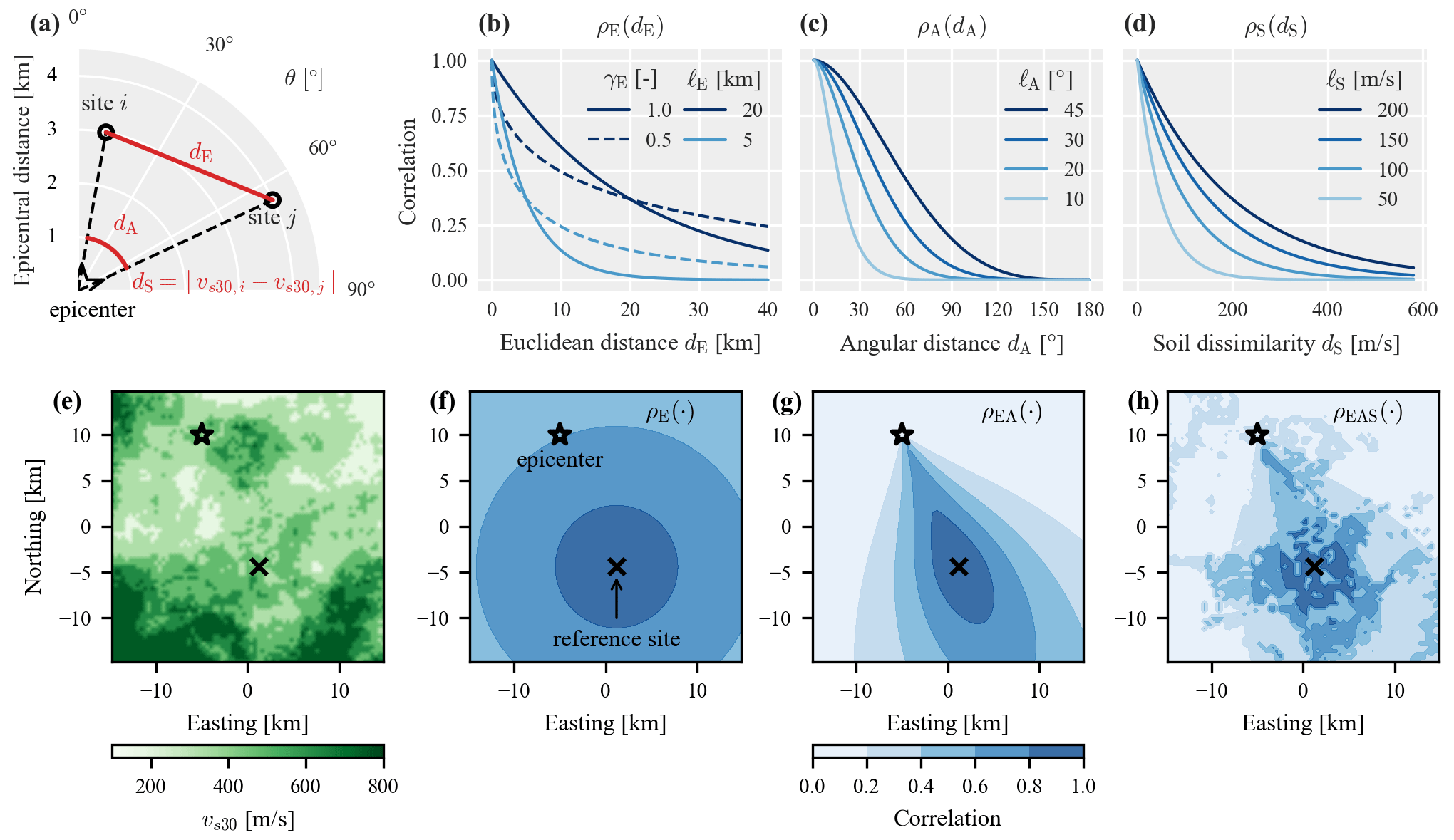
Figure 1 Illustration of the proposed spatial correlation models: distance and dissimilarity metrics (dependent variables) (a) and correlation coefficients as a function of the corresponding dependent variable for different parameters of individual models E, A, and S (b to d). Soil conditions in a fictitious 15×15 km region (e) that are used to illustrate correlation coefficients with respect to the indicated reference site for the combined correlation models E, EA, and EAS (f to h), where the model parameters are set to their corresponding prior mean values stated in Table 1.

2.3 Accounting for site effects using a soil dissimilarity metric

We account for site effects via measuring dissimilarities in local soil conditions following the premise that sites with similar soil conditions have stronger correlations. We use v_s30, the 30 m time-averaged shear-wave velocity, as a proxy for the soil conditions, and the distance metric d_S is the absolute difference in the two sites' v_s30 values. We choose an exponential form of the correlation function:

$$\begin{array}{}\text{(6)}& {\mathit{\rho }}_{\mathrm{S}}\left(d_{\mathrm{S}};{\mathrm{\ell }}_{\mathrm{S}}\right)=\exp \left(-d_{\mathrm{S}}/{\mathrm{\ell }}_{\mathrm{S}}\right),\end{array}$$

where ${\mathrm{\ell }}_{\mathrm{S}}\in {\mathbb{R}}^{+}$ is the length scale (in m s⁻¹). The choice of using v_s30 as a proxy for soil conditions reflects its use in the GMM and its availability in the data sets and case-study regions employed in this study. Other information, such as the depth to bedrock or simply topographic slope (Kotha et al., 2020), could be used in a similar fashion. To simultaneously account for spatial proximity, path, and site effects we introduce correlation model EAS:

$$\begin{array}{}\text{(7)}& \begin{array}{rl}{\mathit{\rho }}_{\mathrm{EAS}}& \left(d_{\mathrm{E}},d_{\mathrm{A}},d_{\mathrm{S}};{\mathit{\psi }}_{\mathrm{EAS}}\right)={\mathit{\rho }}_{\mathrm{E}}\left(d_{\mathrm{E}}\right)\\ & \cdot \left(w{\mathit{\rho }}_{\mathrm{A}}\left(d_{\mathrm{A}}\right)+(\mathrm{1}-w){\mathit{\rho }}_{\mathrm{S}}\left(d_{\mathrm{S}}\right)\right),\end{array}\end{array}$$

where $w\in (\mathrm{0},\mathrm{1})$ is a weight parameter and ${\mathit{\psi }}_{\mathrm{EAS}}=({\mathit{\gamma }}_{\mathrm{E}},{\mathrm{\ell }}_{\mathrm{E}},{\mathrm{\ell }}_{\mathrm{A}},{\mathrm{\ell }}_{\mathrm{S}},w)$ collects all parameters. To illustrate model EAS, Fig. 1h plots the predicted correlation coefficient with respect to the indicated reference site using soil conditions as shown in Fig. 1e. The model still predicts path effects but also higher correlation for sites with similar soil conditions as the reference site.

For model EAS, we explored several combinations of the individual models E, A, and S. Compared to the model defined in Eq. (7), a decrease in predictive performance was observed for the case where the individual components are combined as a weighted sum, whereas the decrease was less pronounced for a purely multiplicative structure. We also tried a model with two separate isotropic components E1 (multiplied with component A) and E2 (multiplied with component S), while Eq. (7) multiplies the same isotropic component E with both A and S. This model had a slightly better predictive performance but comes at the cost of two additional parameters. In favor of reduced model complexity, we decided to proceed with the model specified by Eq. (7).

We note that the herein proposed models focus on correlation of within-event residuals for a single IM at multiple, spatially distributed sites. In future studies, the models may be extended to the case of multiple IMs, for example, through the use of the linear model of co-regionalization as shown in Loth and Baker (2013) for isotropic models.

3 Bayesian parameter estimation

We follow a Bayesian approach to estimate the parameters of the correlation models $\mathrm{M}\in \mathit{\{}\mathrm{E},\mathrm{EA},\mathrm{EAS}\mathit{\}}$, presented in the previous section. Given data 𝒟, we aim to derive the posterior distribution of the correlation model parameters ψ_M using Bayes' theorem:

$$\begin{array}{}\text{(8)}& p\left({\mathit{\psi }}_{\mathrm{M}}\right|\mathcal{D})\propto p(\mathcal{D}\left|{\mathit{\psi }}_{\mathrm{M}}\right)p\left({\mathit{\psi }}_{\mathrm{M}}\right),\end{array}$$

where p(𝒟|ψ_M) denotes the likelihood of jointly observing the data 𝒟 conditional on a correlation model M with a specific parameter set ψ_M, and p(ψ_M) is the prior distribution of the parameters. The individual components of Eq. (8) are introduced in detail in the following sections.

3.1 Data

We consider ground-motion IM data from the NGA-West2 database (Ancheta et al., 2014). The IMs of interest are elastic, 5 % damped spectral accelerations Sa(T) over the range of periods $T\in [\mathrm{0.01},\mathrm{6}]$ s, where we consider the median spectral amplitude over all horizontal orientations (SARotD50). To compute within-event residuals we use the GMM of Chiou and Youngs (2014) and mixed-effects regression (Abrahamson and Youngs, 1992). We restrict the database to consider only ground motions with closest distance to rupture below 300 km, measured or inferred v_s30 values between 180 and 760 m s⁻¹, and a maximum usable period within the period range of interest. We then consider all earthquake events with more than 40 stations that satisfy the above criteria. Besides the computed residuals, z_k, we extract the geo-coordinates s_ki, the epicentral azimuth θ_ki, and v_s30,ki from all records, which we collectively denote as input vector x_ki. The data from event k are denoted as ${\mathcal{D}}_k=({\mathbf{X}}_k,{\mathbf{z}}_k)$, where the inputs and residuals of the stations that recorded event k are summarized in matrix X_k and vector z_k, respectively.

The data set obtained by pooling data from all n_k considered events is denoted as ${\mathcal{D}}_{\mathrm{tot}}=\mathit{\{}{\mathcal{D}}_k\mathrm{|}k=\mathrm{1},\mathrm{\dots },n_k\mathit{\}}$. For Sa(1 s) (spectral acceleration at a period of 1 s), the pooled data set consists of 13 342 records from 128 events. The size of the data sets becomes smaller for spectral accelerations at longer periods due to the maximum usable period limit. Table A1 lists the number of records and events used for each of the considered periods. Figure 2 shows the number of station pairs in bins of Euclidean distance combined with angular distance (a) and with soil dissimilarity (b). As can be seen in Fig. 2a there are only a few station pairs available at short Euclidean distances (smaller than 5 km) and angular distances greater than 60^∘, mainly for two reasons: first, this combination requires data points that have been recorded at short epicentral distances, which are in general scarce; second, for a given Euclidean distance it is more likely that a station pair has small angular distances (i.e., small differences in epicentral azimuths). The number of station pairs available at different combinations of Euclidean distance and soil dissimilarity, shown in Fig. 2b, are more evenly distributed, with relatively few data points from close-by stations with strongly differing soil conditions (e.g., d_S>350 m s⁻¹). Low soil dissimilarity occurs more frequently in this data set, where d_S values larger than 400 m s⁻¹ account for 1.5 % of all station pairs. Additionally, there is a higher likelihood for close-by stations to have similar v_s30 values.

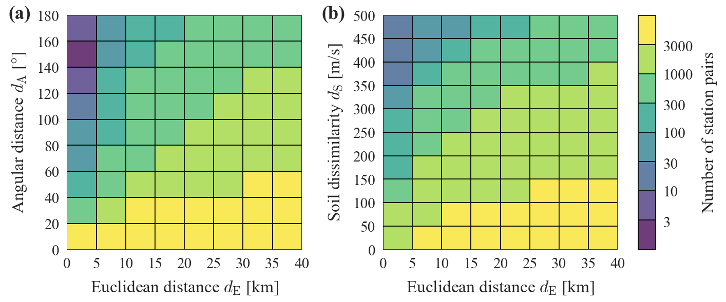
Figure 2 For the pooled training data set for Sa(1 s): number of station pairs in joint bins of Euclidean and angular distance in (a) and number of station pairs in joint bins of Euclidean distance and soil dissimilarity in (b). Note the logarithmic color scale.

3.2 Likelihood

For event k, the likelihood, p(𝒟_k|ψ_M), denotes the joint probability that correlation model M with parameters ψ_M and inputs X_k assigns to scaled within-event residuals z_k computed from the recorded ground-motion IMs as discussed above. This distribution is multivariate normal, so $p\left({\mathcal{D}}_k\right|{\mathit{\psi }}_{\mathrm{M}})=\mathcal{N}(\mathbf{0},\mathbf{\Sigma })$. For the pooled data set 𝒟_tot, we consider the residuals from distinct events to be independent, so the likelihood factorizes: $p\left({\mathcal{D}}_{\mathrm{tot}}\right|{\mathit{\psi }}_{\mathrm{M}})={\prod }_{k}p({\mathcal{D}}_k\left|{\mathit{\psi }}_{\mathrm{M}}\right)$. The joint probability of interest is thus analytically tractable. The correlation model and its parameters ψ_M define the entries of the correlation matrix Σ.

3.3 Prior distributions

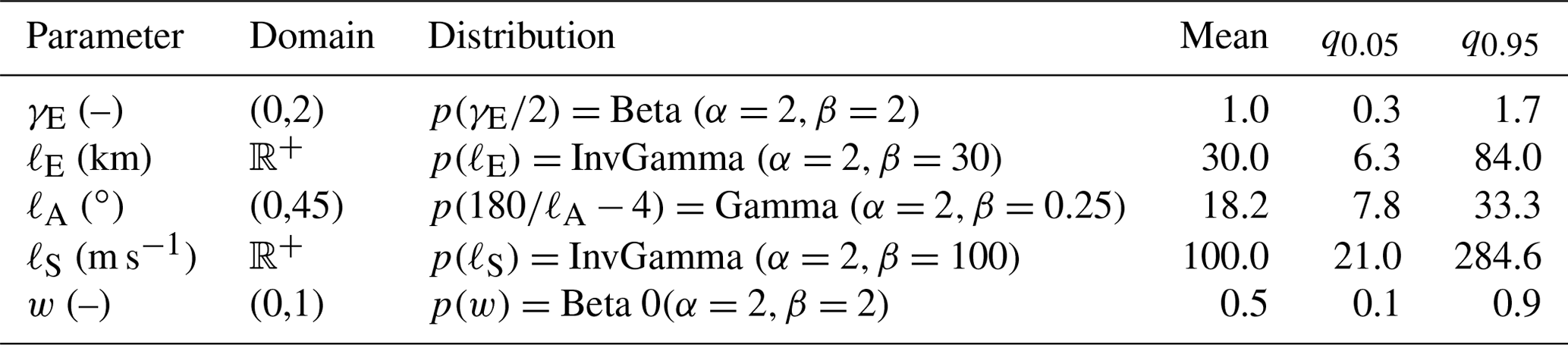
We chose weakly informative prior distributions for the parameters based on guidance provided in Kuehn and Stafford (2021) and Liu et al. (2022b) and assume that their joint distribution, p(ψ_M) in Eq. (8), is factorizing. The prior distributions and the corresponding prior mean, as well as the 5 % and 95 % quantiles, are stated in Table 1. Note that some priors are defined on a scaled version of the parameter to account for its corresponding domain. For instance the exponent γ_E is defined for a range from 0 to 2, which means to get samples of this parameter we first sample from a beta distribution, defined from 0 to 1, and multiply the obtained samples by 2.

Table 1 Prior distributions for the parameters ψ and corresponding means and the 5 % and 95 % quantiles (q_0.05 and q_0.95).

3.4 Posterior distribution

The posterior distribution, p(ψ_M|𝒟) in Eq. (8), is not analytically tractable, and thus we use Markov chain Monte Carlo (MCMC) sampling for Bayesian inference. MCMC is a sequential sampling algorithm that is often used in Bayesian statistics to draw samples from a certain target posterior (Neal, 1993). Specifically, we employ the No-U-Turn Sampler (Hoffman and Gelman, 2014) as implemented in the software library NumPyro (Phan et al., 2019). We get n_r=4000 sampled parameter sets ψ_M,r from the posterior distribution through four independent chains and 1000 warm-up steps each. Additional implementation details can be found in the supplementary online repository (Bodenmann, 2022).

In the following we discuss the estimated parameters by first focusing on isotropic models E that are derived from data 𝒟_k of a single event k, so-called event-specific models. Then we expand the discussion to the case where parameters are estimated from the pooled training data 𝒟_tot, so-called pooled models, where we also include the combined models EA and EAS. The upcoming paragraphs focus on the spectral acceleration at a period of 1 s, Sa(1 s).

3.4.1 Event-specific models

Event-specific correlation models have parameters estimated from data of an individual event. Figure 3 illustrates the joint posterior distributions of the parameters ψ_E estimated separately for three events with an increasing number of records. The top row shows the individual samples ψ_E,r obtained via MCMC and an estimated kernel density for illustrative purposes. The bottom row shows the correlation model evaluated using all sampled parameter sets ψ_E,r.

The results shown in Fig. 3 illustrate differences in the three event-specific models, but they also highlight the uncertainty involved in estimating correlation model parameters from data of individual earthquakes. As pointed out in the Introduction, this estimation uncertainty complicates the identification of factors that could explain the variability in event-specific correlation models. In Sect. 4.1 we will compare the predictive accuracy of such event-specific models to the predictive accuracy of pooled models as introduced in the following.

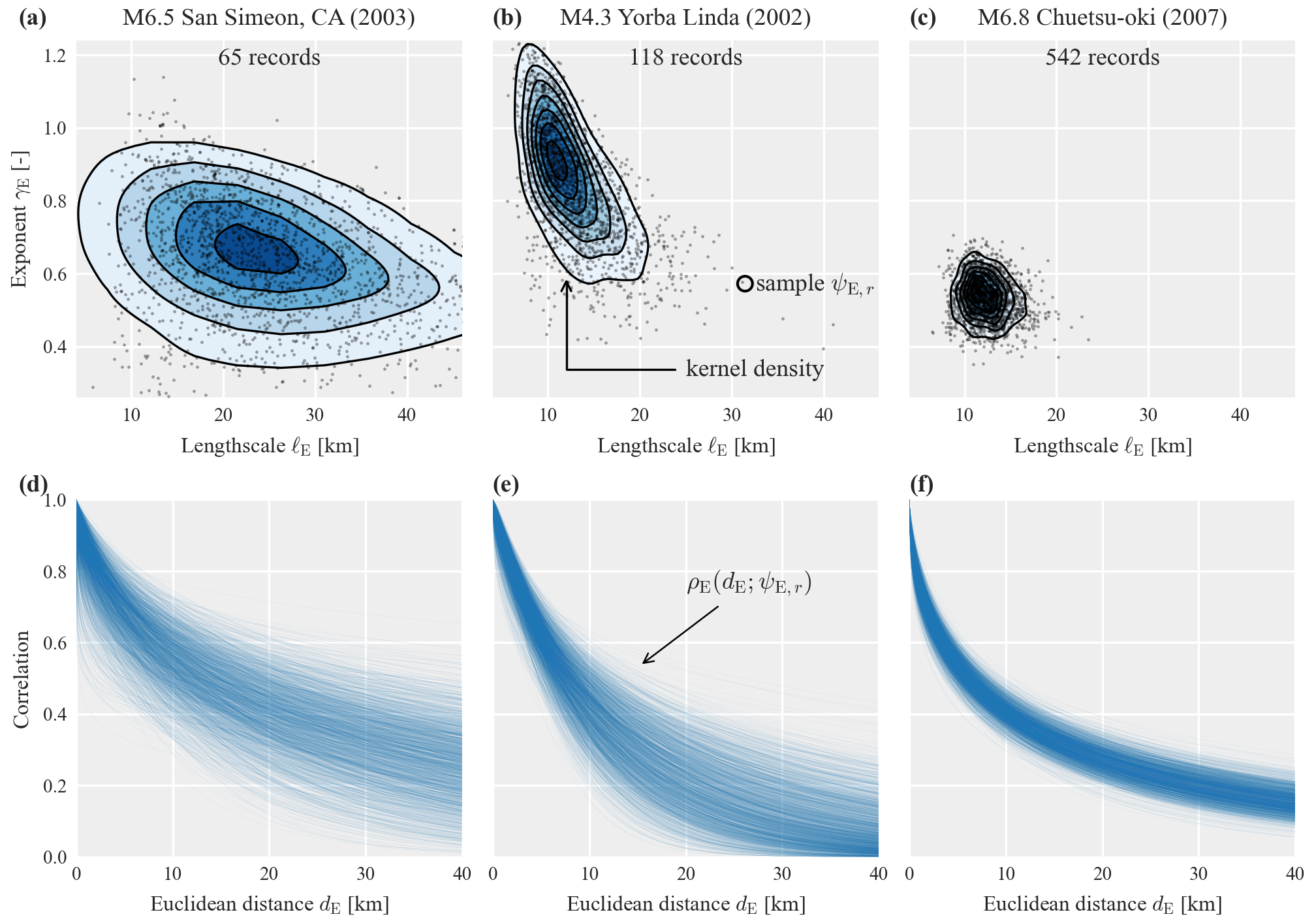
Figure 3 Isotropic model E estimated separately for Sa(1 s) and for three events with increasing number of records: (a)–(c) posterior distributions of the parameters and (d)–(f) predicted correlation coefficients as a function of Euclidean distance for all posterior parameter samples.

3.4.2 Pooled models

Pooled models are derived by combining data from multiple individual earthquakes. In contrast to event-specific models, we use the same parameters to describe correlations of data from all events.

Table 2 summarizes the posterior parameters of correlation models E, EA, and EAS, all inferred from the pooled training data 𝒟_tot. First, we note that the angular length scale, ℓ_A, of models EA and EAS is around 20^∘. As can be seen from Fig. 1c, this means that two sites whose epicentral azimuths differ by more than 90^∘ are essentially uncorrelated. Second, the length scale applied to the Euclidean distance, ℓ_E, is longer for models EAS and EA compared to the isotropic model E, while the exponent γ_E is similar for all three models. Thus, sites with similar azimuthal difference and located on similar soil are correlated over longer Euclidean distances.

For models EAS and E, Fig. 4 illustrates the predicted correlation as a function of Euclidean distance, d_E, for the three soil dissimilarities, d_S, of 10, 100 and 400 m s⁻¹, and at three increasing angular distances, d_A, of 5, 30, and 60^∘. The solid line indicates the function evaluated with the mean posterior parameters, and the shaded area indicates the interval between the 95 % and 5 % quantiles of all sampled functions from the posterior. The isotropic model E depends solely on Euclidean distance, so the predicted correlation is identical in all three panels (a–c). The comparison of this pooled model E to the event-specific isotropic models shown in Fig. 3 reveals the reduction in estimation uncertainty obtained by pooling data from multiple events. For model EAS, on the other hand, we observe increased uncertainty for larger angular distances and short Euclidean distances, which reflects the low amount of data available at such combinations (see Fig. 2). By comparing model EAS in panels (a) and (b), we observe that increasing the angular distance from 5 to 30^∘ has roughly the same effect as increasing the soil dissimilarity from 10 to 400 m s⁻¹. For the plotted range of Euclidean distance, the isotropic model E is similar to model EAS at small angular distances. This is because most data at short distances have small azimuthal differences.

Table 2 Parameters for the different correlation models estimated from the pooled training data set for Sa(1 s). Stated quantities are the mean and the 5 % and 95 % quantiles from the posterior samples.

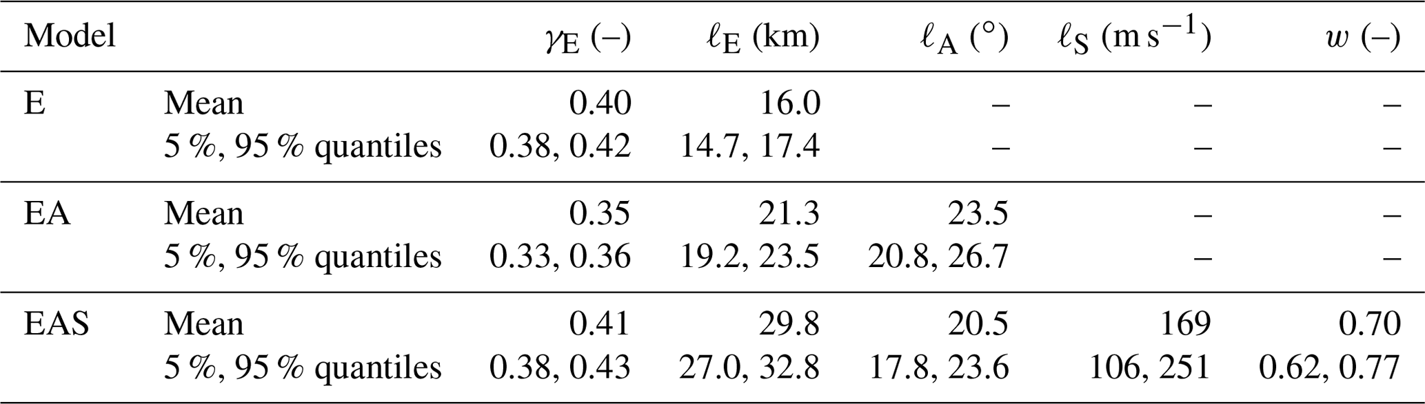
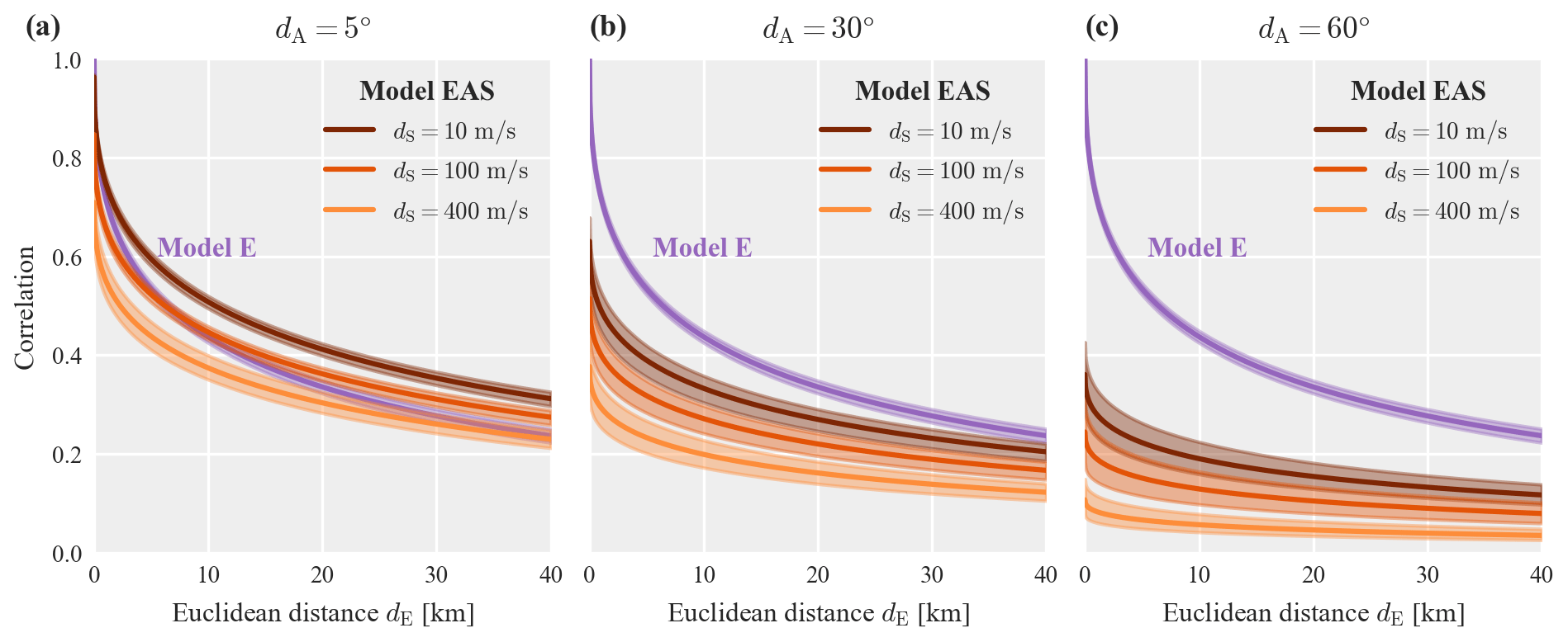
Figure 4 Posterior correlation models EAS and E for Sa(1 s) as a function of Euclidean distance and soil dissimilarity plotted at three angular distances: (a) 5^∘, (b) 30^∘, and (c) 60^∘. The shaded area indicates the interval between the 95 % and 5 % quantiles of all sampled functions from the posterior.

Table A1 in Appendix A presents the parameters of model EAS for “Sa” at eight additional periods, while Fig. A1 provides similar plots as Fig. 4 for Sa(0.3 s) and Sa(3 s). Compared to Sa(1 s), the weight parameter, w, decreases for longer periods, which means the model assigns more weight to the site-effect term (i.e., the term that accounts for soil dissimilarities), compared to the path-effect term (i.e., the term that accounts for angular distances). We further discuss the relative importance of site and path effects in Sect. 4.2.

4 Comparison of model performance

We next evaluate the three models in terms of their predictive accuracy on test data from either an individual event or multiple events. Given the posterior parameters of model M inferred from training data, 𝒟_train, we compute the logarithmic posterior predictive density (LPPD) of test data, 𝒟_test, as

$$\begin{array}{}\text{(9)}& \begin{array}{rl}{\mathrm{LPPD}}_{\mathrm{M}}& ({\mathcal{D}}_{\mathrm{test}};{\mathcal{D}}_{\mathrm{train}})=\ln \int p\left({\mathcal{D}}_{\mathrm{test}}\right|{\mathit{\psi }}_{\mathrm{M}})\\ & p\left({\mathit{\psi }}_{\mathrm{M}}\right|{\mathcal{D}}_{\mathrm{train}})\mathrm{d}{\mathit{\psi }}_{\mathrm{M}}\approx \ln {\displaystyle \frac{\mathrm{1}}{n_r}}\sum _{r=\mathrm{1}}^{n_r}p({\mathcal{D}}_{\mathrm{test}}\left|{\mathit{\psi }}_{\mathrm{M},r}\right),\end{array}\end{array}$$

where ψ_M,r is the rth sample from the posterior p(ψ_M|𝒟_train) obtained via MCMC (Gelman et al., 2014). A higher value of this metric indicates a model that is more compatible with the data, in the sense of predicting higher probabilities of observing the given test data. By marginalizing over the posterior distribution of the parameters, the LPPD takes into account the uncertainty associated with parameter estimation. Because LPPD quantifies the joint predictive density (see Sect. 3.2), it is particularly useful in the context of spatial correlation models. To compare the models we use the relative difference between the LPPD of a model M and the LPPD of a certain baseline model BL:

$$\begin{array}{}\text{(10)}& \mathrm{Rel}.\mathrm{difference}={\displaystyle \frac{{\mathrm{LPPD}}_{\mathrm{BL}}-{\mathrm{LPPD}}_{\mathrm{M}}}{{\mathrm{LPPD}}_{\mathrm{BL}}}}.\end{array}$$

Note that the LPPD is negative (log-scale), thus a positive relative difference indicates that model M has higher predictive accuracy (higher LPPD) than the baseline model BL. The baseline model differs for the different conducted analyses and is specified in the corresponding sections. We performed three analyses in which we consider different test data sets, while the training data always stem from the NGA-West2 database as described in Sect. 3.1. The first two analyses examine the in-sample performance. Specifically, we first focus on Sa(1 s) and compare the performance of pooled models E and EAS (estimated in Sect. 3.4.2) to the performance of event-specific isotropic models E (estimated in Sect. 3.4.1) on data from individual events. Then we analyze the performance of the pooled models on the entire training data set to examine the relative importance of site and path effects in correlation of Sa(T) at different periods T. In the third analysis, we compare out-of-sample performance of the herein proposed correlation models for Sa(1 s) on data not used for training.

4.1 Comparing event-specific and pooled models

As stated in the Introduction, previous studies found that the parameters of an isotropic correlation model estimated from data of different events vary from earthquake to earthquake. To examine this event-to-event variability, we compute for each event k (i) the predictive accuracy LPPD_M(𝒟_k;𝒟_tot) of pooled models $\mathrm{M}\in \mathit{\{}\mathrm{E},\mathrm{EAS}\mathit{\}}$ and (ii) the predictive accuracy LPPD_E(𝒟_k;𝒟_k) of the corresponding isotropic event-specific model.

To illustrate the aforementioned LPPD metrics, we first use 125 records from the Hector Mine earthquake in Fig. 5. The frequency histograms indicate the log-likelihoods computed for individual samples from the posterior distribution of the model parameters, $\ln p\left({\mathcal{D}}_k\right|{\mathit{\psi }}_{\mathrm{M},r})$. The X values indicate the final LPPD metric which is computed from the histogram values as specified in Eq. (9).

We see that the event-specific model E has the largest variance in log-likelihood values, as the model parameters are more uncertain due to limited data, and some sampled parameter values give low probability of observing the data (i.e., low log-likelihoods). For most realizations, however, the event-specific model E outperforms the pooled model E for the given event, as would be expected. By computing the LPPD metric using Eq. (9) we marginalize over the posterior parameters, and the resulting LPPDs of both models are similar, with the event-specific model performing slightly better. We also see that the pooled model EAS has a higher predictive accuracy than both the pooled and event-specific isotropic models E.

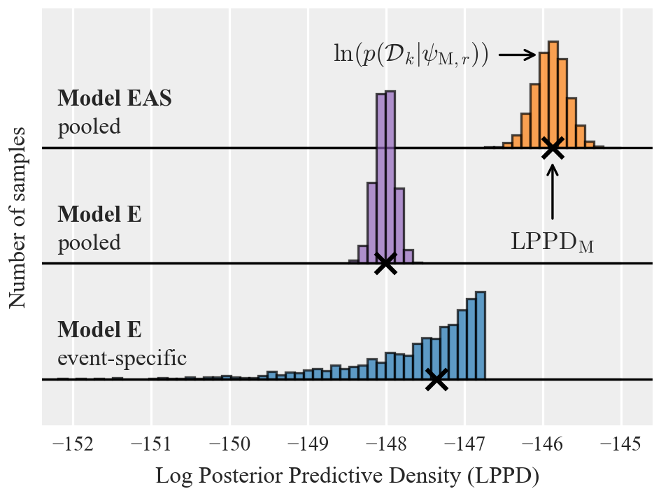
Figure 5 Log posterior predictive density (LPPD) for data from the Hector Mine earthquake event of models E and EAS estimated from the pooled data set, as well as model E with parameters estimated only from data of that event. The histograms show the log-likelihood of the data conditional on samples from the posterior parameters, $\ln p\left({\mathcal{D}}_k\right|{\mathit{\psi }}_{\mathrm{M},r})$.

Figure 6 extends the above comparison to all events in the training data by comparing the LPPDs of pooled model E (panel a) and pooled model EAS (panel b) for each event to the LPPD of the corresponding event-specific isotropic model E using the relative difference metric specified in Eq. (10). The event-specific model E serves as a baseline in computing the relative difference. Thus a positive relative difference indicates that the pooled model predicts the data from that event with higher accuracy than the corresponding event-specific isotropic model.

Figure 6a reveals that the pooled model E has worse predictive accuracy than the event-specific model for most events, with the exception of some events with fewer than 200 records. The exceptions are explained by the increased estimation uncertainty when using sparse data from solely one event, as discussed above. The better predictive accuracy of event-specific models points to event-to-event variability in model parameters when using isotropic correlation models that are only based on Euclidean distance.

On the other hand, Fig. 6b shows that the predictive accuracy of the pooled model EAS is, for most events, higher than the event-specific isotropic model. This is despite the increased number of parameters (and associated estimation uncertainty) and highlights the benefit of accounting for path and site effects in correlation models. It also indicates that the event-to-event variability in correlation model parameters is at least partially explained by the lack of accounting for such effects. Finally, we note that the earthquake magnitude does not seem to affect the relative comparison in LPPDs, neither for model E nor for model EAS.

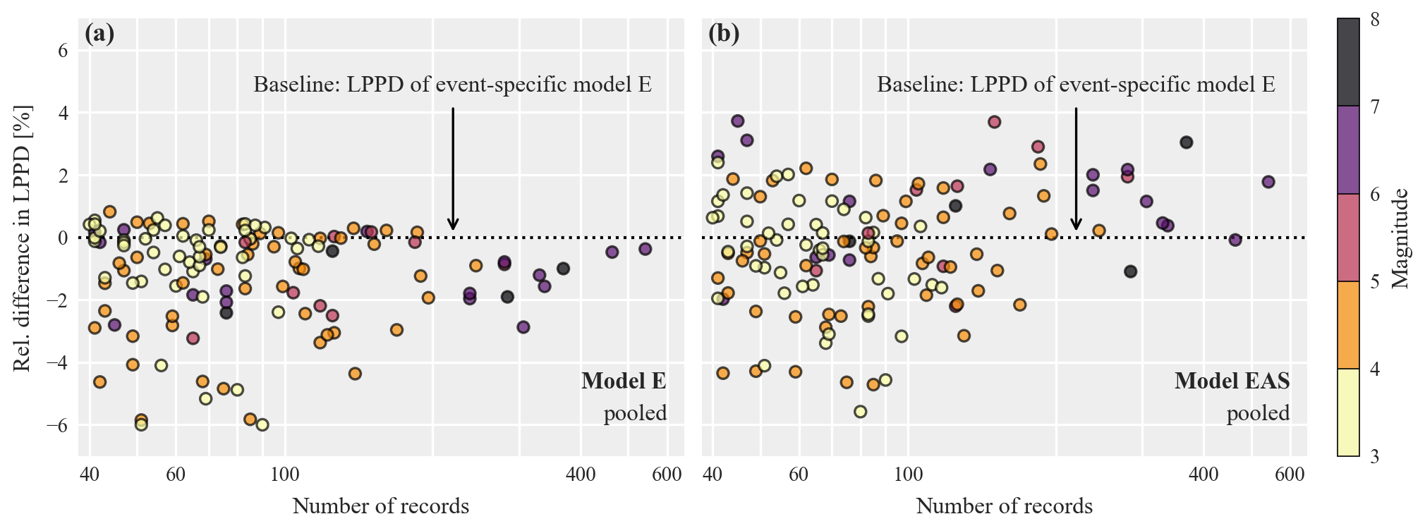
Figure 6 Relative difference in log posterior predictive density (LPPD) of pooled models E (a) and EAS (b) to the LPPD of event-specific models E as a function of the available number of records and magnitude. Each point represents one event in the considered data set, and the coloring indicates the event's magnitude. The relative difference is computed using Eq. (10), and positive values indicate higher predictive accuracy (higher LPPD) of the pooled model for this event compared to the corresponding event-specific model E.

4.2 Pooled model performance for Sa at other periods

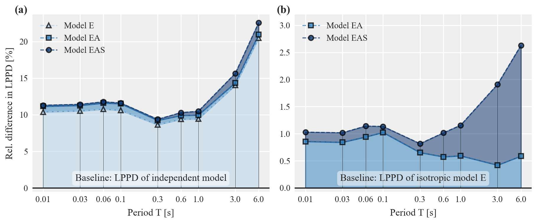
Whereas the previous results considered within-event residuals of Sa(1 s), this section expands the discussion to different periods T. We again use the NGA-West2 data set to estimate parameters of pooled models for residuals at nine periods between 0.01 s and 6 s and evaluate the corresponding LPPD for the entire training data set, LPPD_M (𝒟_tot;𝒟_tot). To enable a comparison across periods we additionally compute the predictive accuracy of an independent model (i.e., no correlation between within-event residuals). For the training data set with n records the latter is computed as ${\mathrm{LPPD}}_{\mathrm{I}}={\sum }_i^n\ln p\left(z_i\right)$, where each individual scaled within-event residual z_i follows a standard normal distribution.

Figure 7a compares the resulting LPPD values in terms of their relative difference to the baseline LPPD of the independent model using Eq. (10). For the considered periods, all three models have increased predictive accuracy compared to the independent model. The major part of the benefit in LPPD stems from the isotropic model E, although accounting for path and site effects (models EA and EAS) leads to further increases in LPPD. Figure 7b focuses on the relative difference of model EA and EAS compared to the baseline of the isotropic model E. Interestingly, for T≤0.3 s the LPPD of model EAS is very similar to the LPPD of model EA. This indicates that, for short periods, additionally accounting for site effects (as measured with model EAS) adds only a minor benefit compared to model EA which only accounts for path effects. For longer periods, however, the site effects become more important. For model EA, Fig. 7b shows larger LPPD for T≤0.1 s compared to longer periods. Further studies are needed to assess whether this indicates more pronounced path effects at shorter periods or whether the chosen functional form in Eq. (4) captures path effects better for shorter periods.

Figure 7 For within-event residuals of Sa(T) at different periods T from the NGA-West2 data set: relative difference (Eq. 10) in log posterior predictive density (LPPD) of pooled models E, EA, and EAS to (a) the LPPD of the independent model and (b) the LPPD of pooled model E.

4.3 Out-of-sample model performance

We use recorded ground-motion data from the 2019 Ridgecrest, California, earthquake sequence (Rekoske et al., 2020) to compare the performance of the herein proposed correlation models on data not used for training, i.e., 𝒟_test⊄𝒟_train. Specifically, we compute the within-event residuals of Sa(1 s) using the regionalized ergodic GMM developed by Liu et al. (2022a). This GMM has been derived using the NGA-West2 database and a subset of 9554 records from 81 earthquakes of the Ridgecrest data set. The latter subset serves here as the first test data set denoted as ${\stackrel{\mathrm{̃}}{\mathcal{D}}}_{\mathrm{1}}$. The second test data set, ${\stackrel{\mathrm{̃}}{\mathcal{D}}}_{\mathrm{2}}$, consists of data from three events with magnitudes 5.4, 6.4, and 7.1 that were not used to fit the GMM. For more details on the ground-motion data and model the reader is referred to Rekoske et al. (2020) and Liu et al. (2022a).

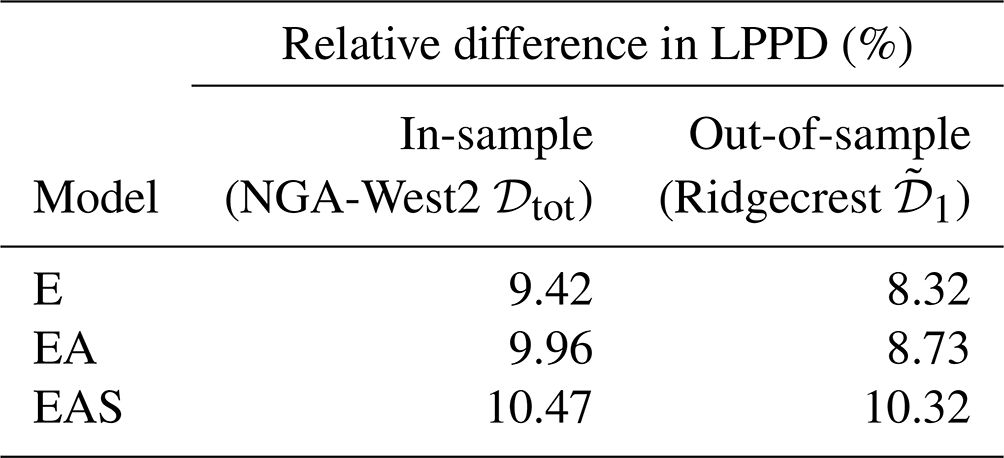
The out-of-sample performance is first assessed via the LPPD of the test set ${\stackrel{\mathrm{̃}}{\mathcal{D}}}_{\mathrm{1}}$ obtained with the pooled correlation models E, EA, and EAS from Sect. 3.4.2. Table 3 shows the resulting relative difference in the LPPDs to the LPPD of an independent model and compares the values to the in-sample performance on the training set. The in-sample values are identical to the results shown in Fig. 7 at period T=1 s. For the test set ${\stackrel{\mathrm{̃}}{\mathcal{D}}}_{\mathrm{1}}$ the increase in LPPD of the model EAS is similar to the in-sample LPPD, whereas the increase in models E and models EA is more than 1 % point smaller. The comparison of models EA and EAS reveals that the additional gain in predictive accuracy obtained from accounting for site effects is larger for the test data (Ridgecrest) than for the training data (NGA-West2).

Table 3 In- and out-of-sample performance in terms of relative difference (Eq. 10) in LPPD of pooled models E, EA, and EAS to the baseline LPPD of an independent model for the training and test data sets.

For the three events in the second test data set, ${\stackrel{\mathrm{̃}}{\mathcal{D}}}_{\mathrm{2}}$, Fig. 8 shows the computed within-event residuals in the top row and the relative difference in LPPD compared to the corresponding independent model in the bottom row. Similar to Fig. 5, the histograms show the log-likelihood of the different models conditional on samples from the posterior distributions of parameter values, whereas the X marks the marginalized LPPD. For all three events, model EAS has a higher predictive accuracy than the isotropic model E.

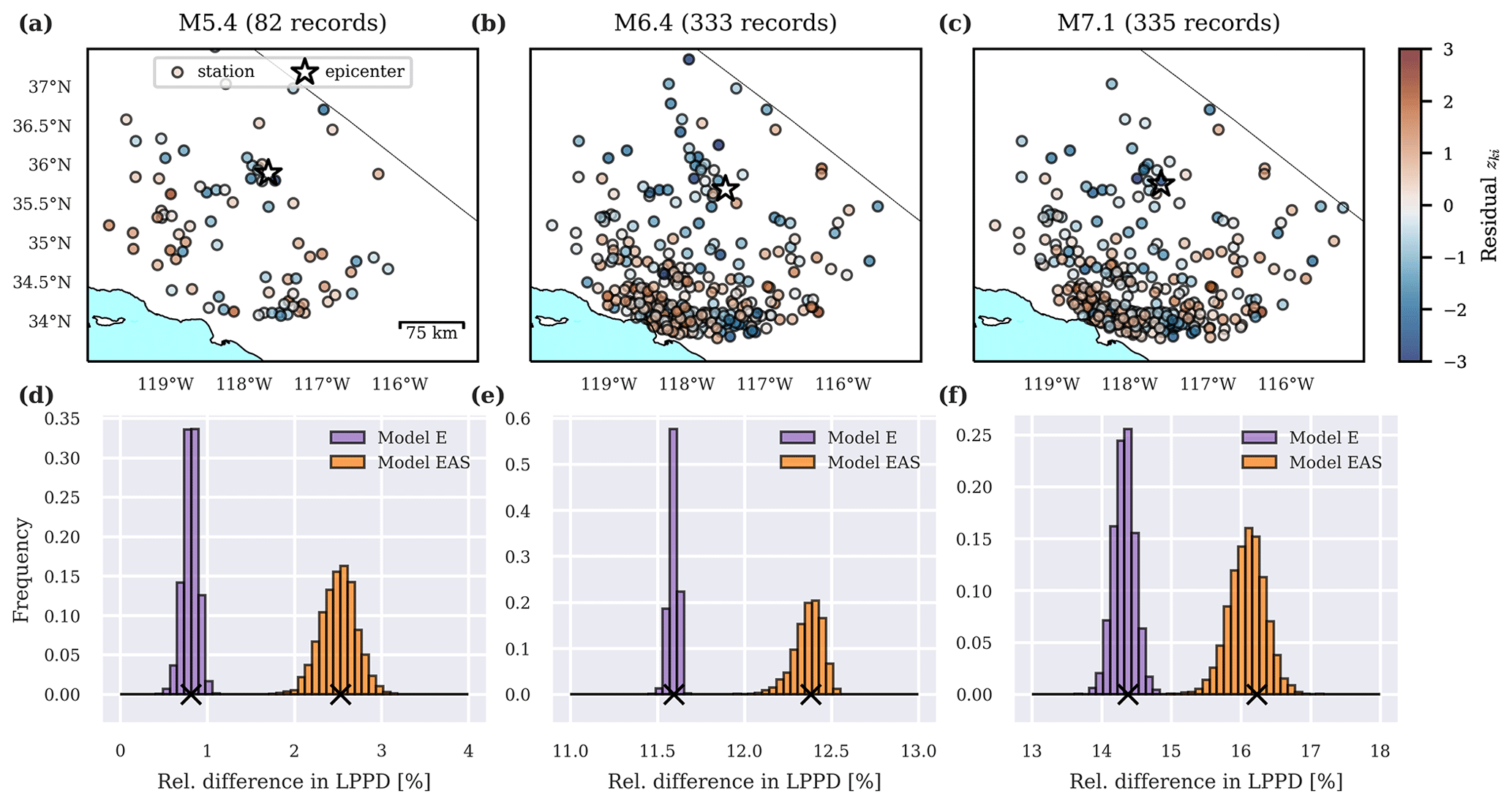
Figure 8 For the three earthquakes in the second test set from the 2019 Ridgecrest sequence: the spatial distribution of scaled within-event residuals z_k of Sa(1 s) (a–c) and the relative difference (Eq. 10) in log posterior predictive density (LPPD) of pooled models E and EAS to the baseline LPPD of the independent model (d–f).

5 Implications for regional seismic hazard and risk

Figure 9a shows the configuration of a simplified case study to assess the implications of the different correlation models for regional seismic risk simulations. Four 5×5 km subregions are located in the San Francisco Bay Area, California, subjected to a M6.25 rupture on the Hayward fault. As a first visual comparison of the estimated models E and EAS, Fig. 9b and c show maps of computed correlation coefficients from the indicated reference site to all other sites. According to model EAS, sites in subregion two are essentially uncorrelated to the reference site, while model E predicts a correlation between 50 % and 60 %.

Next, the four subregions are gridded into individual sites with a spacing of 3 arcsec (approximately 90 m). The quantity of interest is the proportion of sites, a, within one or several subregions, where the Sa(1 s) jointly exceeds a certain threshold value sa, which we denote as random variable A_Sa(1 s)>sa. While regional seismic risk is typically quantified in terms of fatalities, financial losses or downtime, the joint distribution of Sa values is a major component in the underlying workflow and an important driver of such regional seismic risk metrics (Weatherill et al., 2015). As such, the presented results provide initial, but certainly not complete, information on potential implications of the proposed correlation model for regional seismic risk simulation.

The rupture scenario is taken from the UCERF2 earthquake rupture forecast (Field et al., 2008). We use OpenSHA (Field et al., 2003) to compute the mean ln Sa value at all sites, as well as the between- and within-event standard deviations, τ and ϕ, from the GMM of Chiou and Youngs (2014). The v_s30 values, illustrated in Fig. 9a, are obtained from Thompson (2022). Then we sample scaled within-event residuals z from the posterior predictive distribution p(z|𝒟_tot) and multiply them with the within-event standard deviation ϕ to get samples of δW. For δB we sample from a zero-mean normal distribution with standard deviation τ. Finally, we obtain sampled ground-motion fields by summing the mean ln Sa value and the sampled residuals using Eq. (1) and compute a sample of A_Sa(1 s)>sa by counting the number of sites where the simulated ground-motion field exceeds a certain threshold value sa. We compute site-specific thresholds such that they have an identical 10 % probability of being exceeded in the considered scenario.

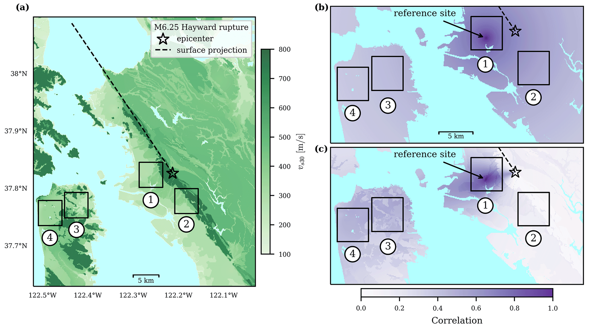
Figure 9 Map of the case study area used for regional risk assessment and the considered M6.25 rupture on the Hayward fault: (a) soil conditions, quantified via v_s30, and correlation coefficient from the indicated reference site to all other sites obtained with posterior mean parameters of model E (b) and model EAS (c). Numbered boxes indicate the subregions of interest (blue areas are water).

Note that the above process requires realizations of z from each sampled parameter set from the posterior ψ_M,r obtained via MCMC. This sampling from the posterior predictive distribution is computationally expensive because, for each ψ_M,r, it requires the evaluation of a novel covariance matrix and a subsequent sampling from the corresponding multivariate normal. Thus, we first explore whether it is sufficient to use the mean values from the posterior distribution of each parameter to build one covariance matrix and generate all samples from that corresponding multivariate normal. Figure 10 compares the resulting exceedance probability curves for the proportion of sites in subregion two where Sa(1 s), induced by the considered scenario rupture, jointly exceeds the specified thresholds. To calculate the exceedance probability curves, we used the posterior parameters from model EAS because this model has more parameters and increased estimation uncertainty compared to model E (as shown in Fig. 4). We observe that the exceedance probability curves obtained via both approaches are visually identical. The same comparison for the other subregions produced the same findings. This indicates that the less expensive approach of using the mean posterior parameters is sufficient for these regional risk estimates.

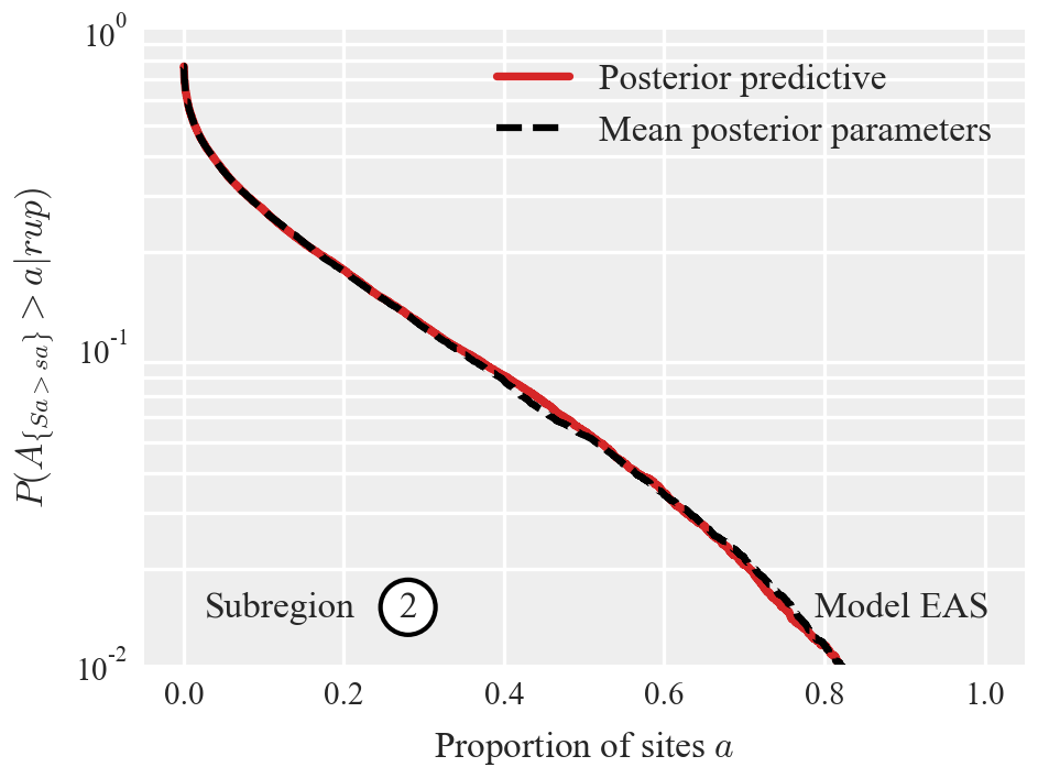
Figure 10 Exceedance probability curves for the proportion of sites a in subregion two where Sa(1 s) jointly exceeds the site-specific thresholds, obtained via sampling from the posterior predictive distribution of model EAS (dashed line) and sampling conditional on the mean values of the posterior parameter distributions (solid line).

We used the posterior mean parameters of model E and model EAS to compute exceedance probability curves for the proportion of sites within the different subregions where Sa(1 s) jointly exceeds the 10 % exceedance probability thresholds. Figure 11 shows results for subregions one and two (top row) and subregions three and four (bottom row). Experiments with different fixed threshold values did not change the conclusions.

In subregions with differing epicentral azimuth values and heterogeneous soil conditions (top row), the isotropic model E predicts stronger correlations and thus heavier tailed distributions (i.e., higher probabilities of jointly exceeding the threshold value at a high proportion of sites). This is especially apparent if subregions one and two are combined (Fig. 11c), where the probability of jointly exceeding the threshold value at least at 40 % of all sites is 9.5 % for model E and only 5.5 % for model EAS. If subregions three and four are combined (Fig. 11f), the exceedance probability curves from both models are similar because these subregions are located at similar azimuths from the epicenter and the assigned correlation coefficients are similar for both models (see Fig. 4a). For subregion four (Fig. 11e), the curve obtained via model EAS has slightly heavier tails compared to the one of model E, which may be explained by the homogeneous soil conditions in this subregion (see Fig. 9).

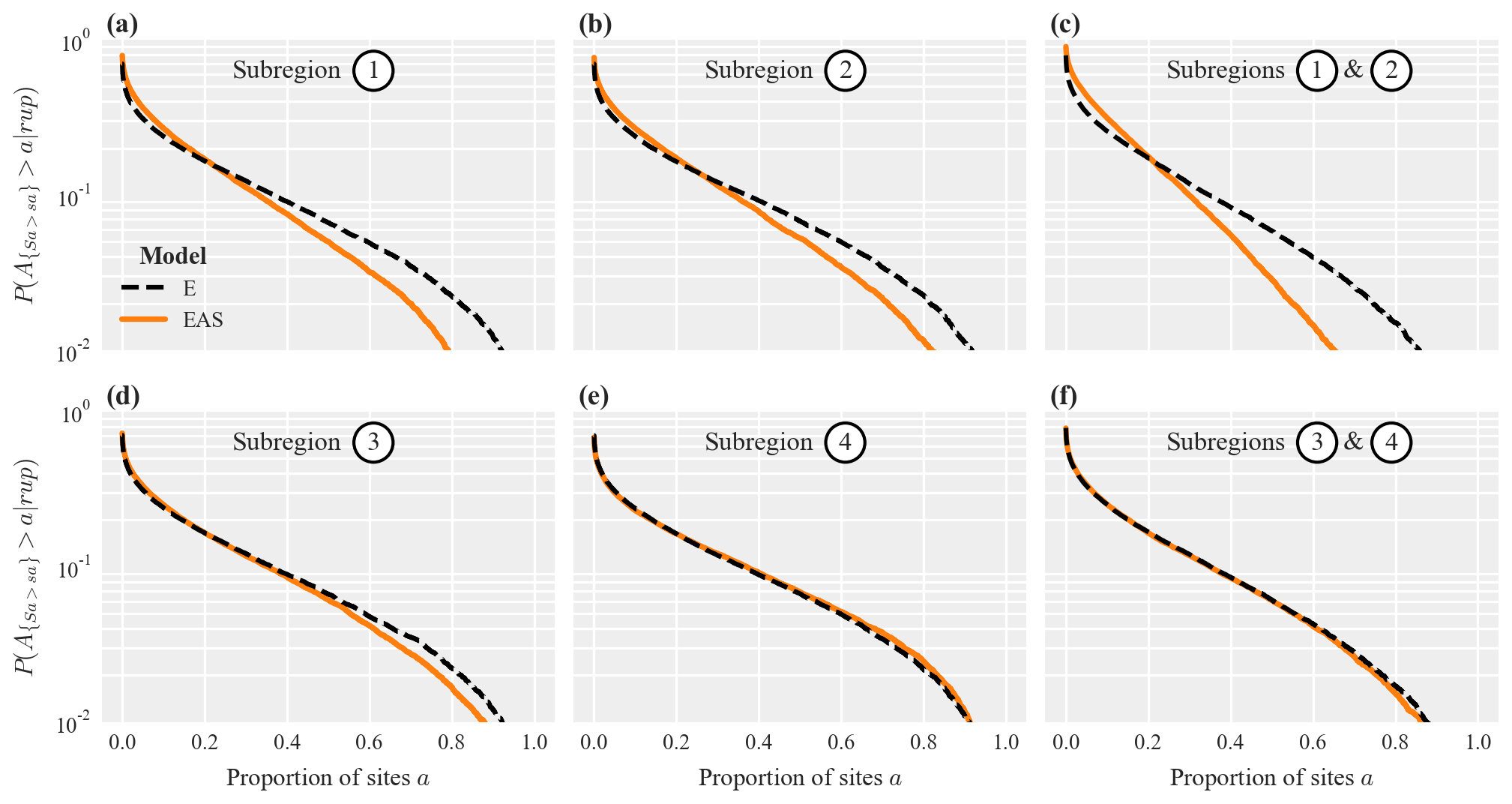
Figure 11 Exceedance probability curves for the proportion of sites a in the considered subregions where Sa(1 s) jointly exceeds a threshold value sa: for subregions one and two separately (a, b) and for one and two combined (c) using a threshold value of 0.75 g, as well as for subregions three and four using a threshold value of 0.25 g (d–f) .

Figure B1 in Appendix B compares the results for Sa(1 s) (shown in Fig. 11) to results obtained for Sa(0.3 s) and Sa(0.6 s). This comparison aligns well with our discussion on the relative importance of site and path effects in Sect. 4.2, and we refer to Appendix B for a brief discussion.

6 Conclusions

This study explored the role of spatial proximity, local site effects, and path effects on spatial correlations of recorded ground-motion intensity measures. The motivation for this work came from the substantial event-to-event variability found in the correlation model parameters estimated in previous studies, as well as questions as to whether such variability was due to event-specific characteristics or due to model and estimation uncertainty. Site and path effects are qualitative contributors to spatial correlations but were not captured by the isotropic correlation models used in previous studies: thus, our focus is on the path and site effects to explain the observed model parameter variability.

We proposed a novel correlation model, EAS, that accounts for path and site effects in addition to spatial proximity. The EAS model assigns decreasing correlation coefficients for sites with increasing Euclidean distance, increasing angular distance, and increasing soil dissimilarity. These three model components reflect the role of spatial proximity, path effects, and site effects, respectively, on spatial ground-motion correlations. Compared to an isotropic model, the proposed model has increased complexity and more parameters (five instead of one or two for the isotropic model). To account for this increase in model complexity, we employ Bayesian inference to estimate the parameters, and we assume that the same parameters describe the correlation for all events in the considered ground-motion database (i.e., a pooled model).

For each event in the NGA-West2 training data set, we then computed the predictive accuracy of the proposed EAS model, as well as of two isotropic models E, where the parameters of one model were estimated from the pooled data set, and the others exclusively consider data from that specific event. For most events, we found that the event-specific models E have higher predictive accuracy then the pooled model E, thus confirming the presence of some event-to-event variability in correlation model parameters. However, the pooled model EAS outperforms the event-specific models E for the majority of events and, especially, for the well-recorded events. This indicates that the event-to-event variability in estimated isotropic model parameters found in previous studies is an apparent variability due to estimation uncertainty and the lack of accounting for site and path effects rather than a true variability. Data from the 2019 Ridgecrest earthquake sequence were then used to compare the models in terms of their out-of-sample performance. The results showed a higher predictive accuracy for model EAS compared to the isotropic model E, further highlighting the benefit of accounting for site and path effects in correlation models.

We then used a case study to explore the implications of using the different correlation models for regional seismic risk simulations. First, we found that generating correlated ground-motion samples using the mean values from the posterior distribution of each parameter instead of sampling from the posterior predictive distribution produces ground-motion fields with practically equivalent distributions. This is helpful because it is much less computationally expensive to use mean parameter values. Second, we saw that the isotropic model E predicts substantially stronger correlations than model EAS in regions with heterogeneous soil conditions and varying epicentral azimuths. This may lead to an overestimation of regional seismic risk tails (low-probability, high-consequence events), particularly in regions located close to the earthquake source.

The proposed model and analysis could benefit from some further study. This could include a refined model parameterization to consider an azimuth metric that accounts for finite-fault effects or to consider other metrics of dissimilarity in site conditions. The refined EAS model could also be tested on more complex risk analysis problems to further understand the practical impact of these refinements. Despite those opportunities for further study, the proposed EAS model form and the proposed techniques for evaluating model performance should be of general use for analysts interested in studying and improving the prediction of spatial correlations in ground motions.

Appendix A: Posterior correlation models for Sa at other periods

Table A1 Parameters for correlation model EAS estimated for Sa at nine periods from the pooled training data set with indicated number of records, n_r, and events, n_e. Stated quantities are the mean (m.) and the 5 % and 95 % quantiles from the posterior samples.

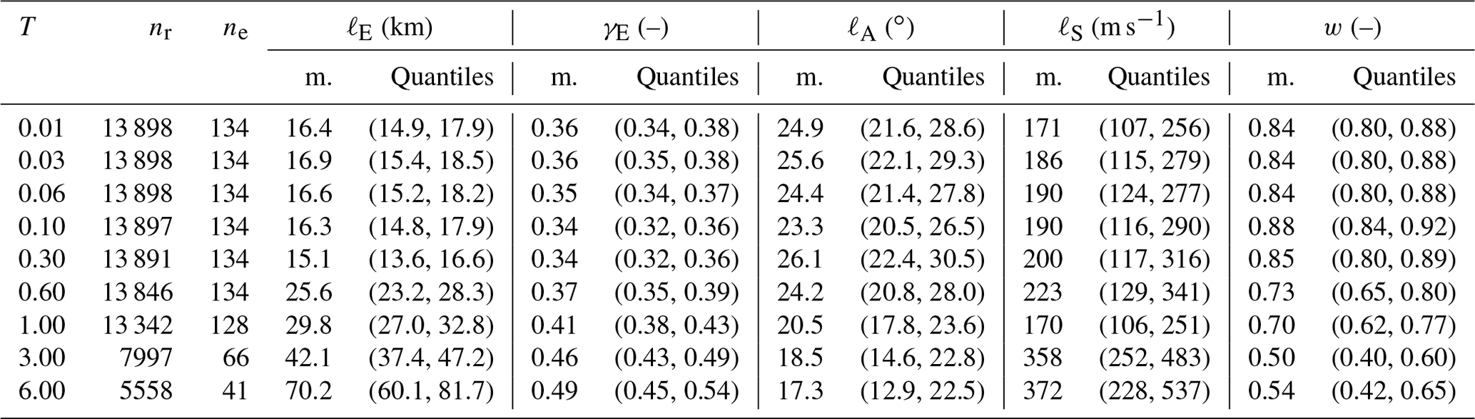
This appendix provides additional results for the pooled model EAS. Table A1 shows the parameters of the proposed correlation model EAS for Sa at nine periods, which are also available in the Supplement (Bodenmann, 2022). Figure A1 compares models EAS and E for Sa(0.3 s) and Sa(3 s).

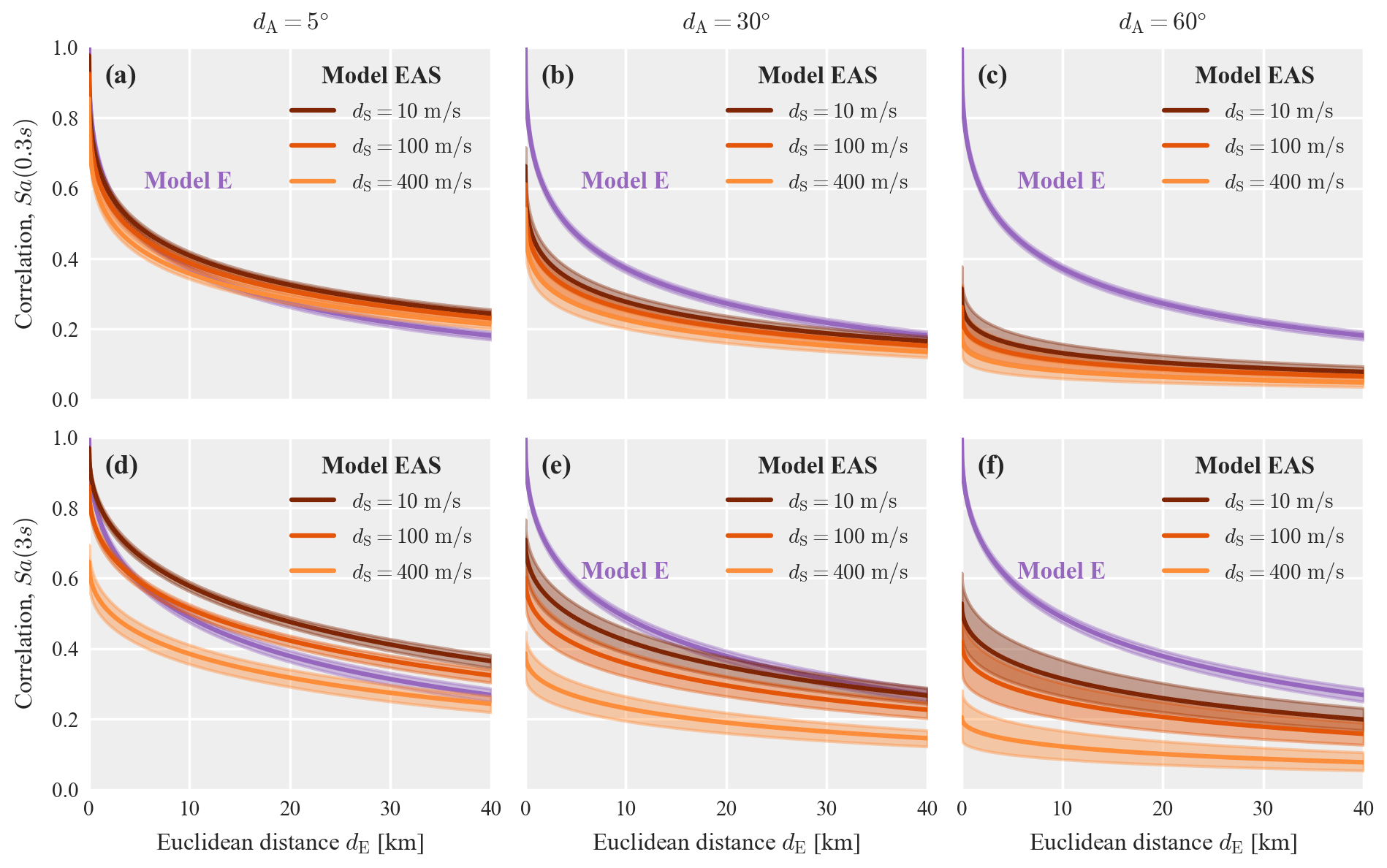
Figure A1 Posterior correlation models EAS and E for Sa(0.3 s) (a–c) and Sa(3 s) (d–f) as a function of Euclidean distance and soil dissimilarity plotted at three angular distances: (a, d) 5^∘, (b, e) 30^∘, and (c, f) 60^∘. The shaded area indicates the interval between the 95 % and 5 % quantiles of all sampled functions from the posterior.

Appendix B: Case study results for Sa at other periods

Figure B1 compares the results for Sa(1 s) (shown in Fig. 11) to results obtained for Sa(0.3 s) and Sa(0.6 s). For subregions one and two (panel c), the difference in the exceedance probability curves from models E and EAS are smaller for the longer period of 3 s due to site effects becoming more important than path effects; i.e., the decrease in correlation because of differing epicentral azimuths is less pronounced. For subregion four (panel e), the curves from models E and EAS are practically identical for Sa(0.3 s), while model EAS has slightly heavier tails for longer periods due to the homogeneous soil conditions.

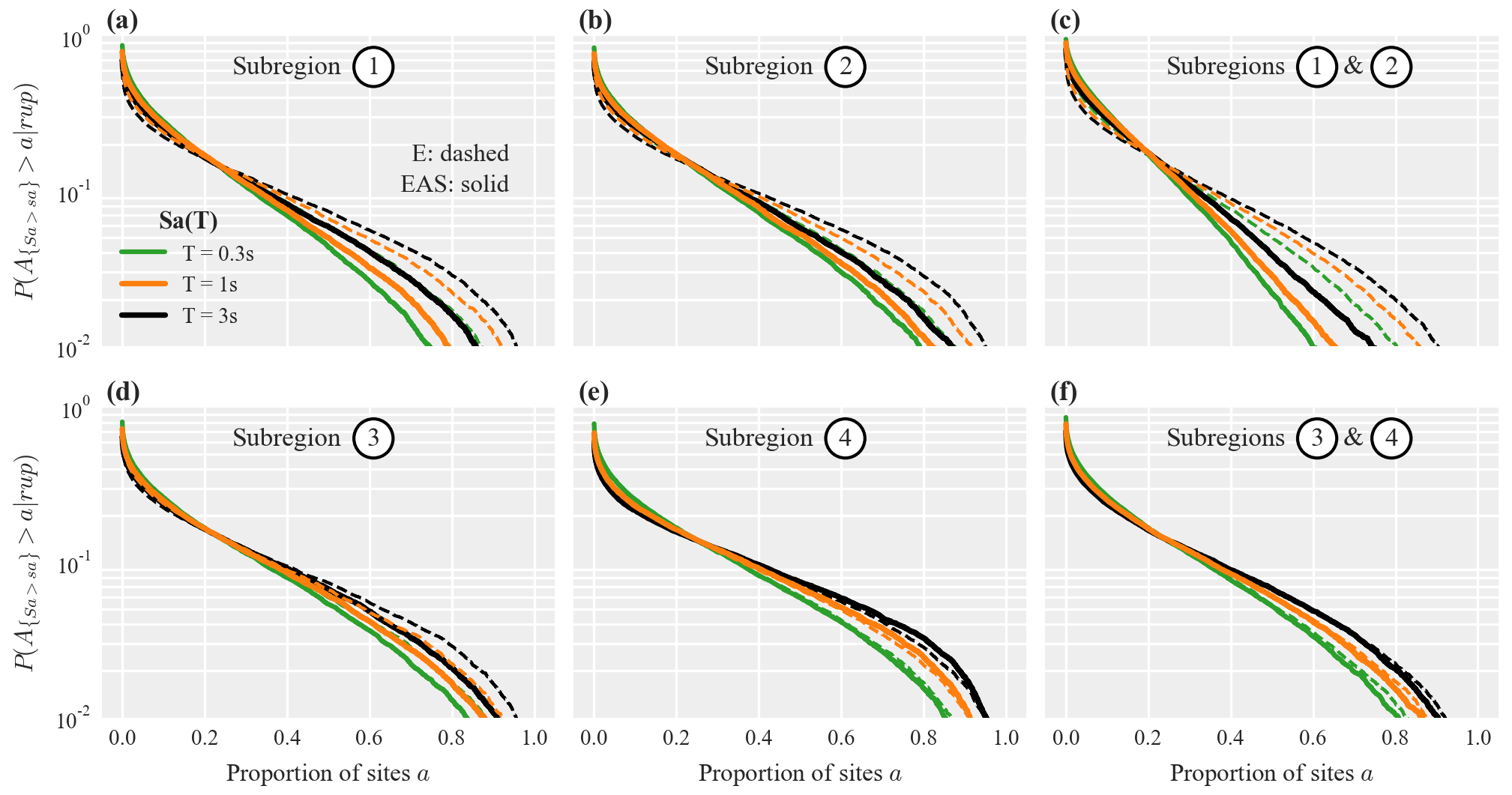
Figure B1 Exceedance probability curves for the proportion of sites a in the considered subregions where Sa(T) jointly exceeds a threshold value sa. Solid and dashed lines plot results for models E and EAS, respectively, while the colors indicate different periods $T\in \mathit{\{}\mathrm{0.3},\mathrm{1},\mathrm{3}\mathit{\}}$ s. Thresholds are computed such that at each site there is a 10 % probability that sa is exceeded for the rupture scenario shown in Fig. 9a.