A predictive equation for wave setup using genetic programming

We applied machine learning to improve the accuracy of present predictors of wave setup. Namely, we used an evolutionary-based genetic programming model and a previously published dataset, which includes various beach and wave conditions. Here, we present two new wave setup predictors: a simple predictor, which is a function of wave height, wavelength, and foreshore beach slope, and a fitter, but more complex predictor, which is also a function of sediment diameter. The results show that the new predictors outperform existing formulas. We conclude that machine learning models are capable of improving predictive capability (when compared to existing predictors) and also of providing a physically sound description of wave setup.

1 Introduction

As the climate changes, coastal flooding is predicted to increase worldwide. Among the processes included to determine coastal flooding, wave runup is recognized as one of its major contributors. Defined as the maximum vertical excursion of water above the mean water level, wave runup represents the action of the waves on the beach face. It comprises two different processes: wave setup and swash. Its importance can be highlighted by the fact that neglecting the wave contribution to coastal flooding can result in up to a ∼60 % underestimation of the flooded area (Vousdoukas et al., 2016).

Wave setup (hereafter referred to simply as setup) is defined as the time-averaged additional elevation of the water level due to breaking waves (Longuet-Higgins and Stewart, 1964). As waves approach the shoreline, their action induces the cross-shore transport of momentum, producing changes in pressure and velocity. To conserve the flow of momentum when meeting obstacles, like a sloping beach, it is necessary to account for the action of a force known as radiation stress. Variations in radiation stress result in a rise (setup) and fall (set-down) in the mean water level. Maximum set-down occurs at the wave's breaking point and decays seaward from that point, whereas setup develops in the shoreward direction (Bowen et al., 1968).

Besides being an important component of coastal flooding (Vitousek et al., 2017; Melet et al., 2020) directly impacting the design of coastal structures, setup is also important to the nearshore circulation, including undertow currents and groundwater flows (Longuet-Higgins, 1983). Ultimately, setup is an important component in the flow and sediment exchanges between the sub-aerial and submerged beach face. Thus, understanding and being able to predict wave setup is vital to protect coastal resources and the population living near the shore in a more effective way.

The setup contribution to extreme water levels was first noticed in 1938 during a hurricane on the east coast of the USA, where a water level 1 m higher than in calm water conditions was observed on an exposed beach (Saville, 1961). After this event, many laboratory experiments and field measurements were conducted to predict setup across the surf zone (Bowen et al., 1968; Battjes, 1974; Guza and Thornton, 1981; Holman and Sallenger, 1985; King et al., 1990; Yanagishima and Katoh, 1990; Hanslow and Nielsen, 1993; Raubenheimer et al., 2001; Stockdon et al., 2006; Ji et al., 2018; O'Grady et al., 2019). As a result, empirical setup predictors based on wave parameters, beach morphology, and surf zone processes have been developed (Dean and Walton, 2009; Gomes da Silva et al., 2020). Some of the most relevant will be presented next.

In one of the first studies about setup, Bowen et al. (1968) conducted a laboratory investigation with monochromatic waves. Their results indicated that the theory, based on the concept of radiation stress, underpredicts measured setup values, especially at the shoreline. The maximum setup (${\stackrel{\mathrm{‾}}{\mathit{\eta }}}_{\mathrm{M}}$), time-averaged elevation of the water level at the shoreline, became the focus of subsequent studies.

Battjes (1974) performed laboratory experiments estimating maximum setup as

$$\begin{array}{}\text{(1)}& {\stackrel{\mathrm{‾}}{\mathit{\eta }}}_{\mathrm{M}}=\mathrm{0.38}\mathit{\gamma }{H}_{\mathrm{b}},\end{array}$$

where H_b is the breaking wave height and $\mathit{\gamma }=H/(\stackrel{\mathrm{‾}}{\mathit{\eta }}+h)$ assumes that the ratio between the height of a broken wave or bore (H) and the water depth (h) remains approximately constant. King et al. (1990), using the same linear function of incident wave height replacing H for H_rms (root mean square), was also able to accurately predict setup for a random wave field. However, the authors (and later Guza and Thornton, 1981) highlighted the fact that γ values in laboratory experiments are higher than in field observations.

Through field data measured on a gently sloping beach, Guza and Thornton (1981) correlated maximum setup to the offshore significant wave height (H_s0):

$$\begin{array}{}\text{(2)}& {\stackrel{\mathrm{‾}}{\mathit{\eta }}}_{\mathrm{M}}=\mathrm{0.17}{H}_{\mathrm{s}\mathrm{0}}.\end{array}$$

This predictor underestimated setup at the shoreline, further suggesting that the slope of the setup is not constant across the surf zone, as described in previous works (Bowen et al., 1968; Battjes, 1974). Later, Holman and Sallenger (1985) found a more accurate correlation than the one presented by Guza and Thornton (1981) by relating the setup with the surf similarity parameter (Iribarren number: ${\mathit{\xi }}_{\mathrm{0}}={\mathit{\beta }}_{\mathrm{f}}/(H_{\mathrm{s}\mathrm{0}}/L_{\mathrm{0}}{)}^{\mathrm{0.5}}$, where β_f is the foreshore slope, $H_{\mathrm{s}\mathrm{0}}/L_{\mathrm{0}}$ is the wave steepness and L₀ the offshore wavelength). However, when isolating low tide data, no significant trend was found with ξ₀, indicating the probable setup dependency on the entire surf zone's bathymetry and not only on the foreshore slope. The same linear relationship between setup and offshore wave height, influenced by tidal fluctuations and the local bathymetry, was also found by Raubenheimer et al. (2001).

Considering the difficulty of defining the parameters used in the predictors above for natural beaches (opposite to laboratory environments), Stockdon et al. (2006) proposed a simple empirical parameterization for setup:

$$\begin{array}{}\text{(3)}& {\stackrel{\mathrm{‾}}{\mathit{\eta }}}_{\mathrm{M}}=\mathrm{0.35}{\mathit{\beta }}_{\mathrm{f}}(H_{\mathrm{s}\mathrm{0}}{L}_{\mathrm{0}}{)}^{\mathrm{0.5}}.\end{array}$$

This equation was based on an extensive dataset, 10 experiments from the USA and the Netherlands, comprising a variety of beach characteristics and wave conditions. As a result, Stockdon et al. (2006) found setup is best parameterized when considering offshore over onshore wave hydrodynamics and using the foreshore slope instead of the surf zone slope. Moreover, for fully dissipative conditions, the inclusion of β_f in the parameterization appears to be unnecessary. The role of deep water waves and the inclusion of foreshore slope at steeper beaches had also been previously recognized by Hanslow and Nielsen (1993).

Recently, Ji et al. (2018) proposed an empirical formula for maximum setup based on different beach slopes and wave parameters through the use of a coupled wave–current model over a linear bathymetry. Besides beach slope, their results showed that setup is also related to wave steepness:

$$\begin{array}{}\text{(4)}& {\stackrel{\mathrm{‾}}{\mathit{\eta }}}_{\mathrm{M}}=\mathrm{0.220}\left({\mathit{\beta }}_{\mathrm{s}}{)}^{\mathrm{0.538}}{H}_{\mathrm{s}\mathrm{0}}\right({\displaystyle \frac{H_{\mathrm{s}\mathrm{0}}}{L_{\mathrm{0}}}}{)}^{-\mathrm{0.371}},\end{array}$$

where β_s is beach slope. Similar results confirming the role of wave height, beach slope, and wave steepness on maximum setups were found by Yanagishima and Katoh (1990) and O'Grady et al. (2019). O'Grady et al. (2019) tested different empirical equations and identified that deep water wave height explains 30 % of setup variance, followed by an improvement of up to 12 % if beach slope is added to the relationship and a further 12 % when including wave steepness. Presently, among all studies providing empirical predictors of setup, the most widely used formulation is the one from Stockdon et al. (2006).

Despite an approximately linear relationship between setup at the shoreline and wave height, traditional setup estimates usually do not account for all the complex processes involved in the environment, often translating into significant scatter in predictions (Stephens et al., 2011; Stockdon et al., 2006; Gomes da Silva et al., 2020). Additional factors that may affect the accuracy of setup predictors include possible errors in the measurements (Guza and Thornton, 1981; King et al., 1990; Lentz and Raubenheimer, 1999), misinterpreted average position of the waterline and difficulty in detecting the maximum setup (Guza and Thornton, 1981; Holman and Sallenger, 1985; King et al., 1990; Lentz and Raubenheimer, 1999), as well as simplifications and uncertain or unaccounted terms such as bottom stress, alongshore bathymetric features, and infragravity waves (Lentz and Raubenheimer, 1999; Ji et al., 2018; O'Grady et al., 2019). In an attempt to overcome these problems and reduce scatter, innovative data-driven approaches, such as machine learning, are becoming increasingly popular since they can provide rapid and accurate predictions (Goldstein et al., 2019; Beuzen and Splinter, 2020).

Machine learning (ML) is a field of computer science focused on developing algorithms that discover relationships between variables by self-improving predictive performance based on a given dataset, without being explicitly programmed to solve that particular problem. Over the past few years, published works have explored the range of applicability of ML approaches, resulting in higher performance and more cost-effective predictors (Goldstein et al., 2019). In coastal sciences, some of the most widely used techniques are k-nearest neighbours, decision trees, random forests, Bayesian networks, artificial neural networks, and support vector machines (Beuzen and Splinter, 2020). A lesser known, yet powerful, algorithm that can provide further insights into the impacts of the underlying processes is genetic programming (GP). One of the main advantages of this approach is the ability to develop reliable, robust, and reproducible predictors. Moreover, it is proven to be a powerful technique capable not only of improving predicting capability but also of being interpretable and potentially providing insight into coastal processes (Passarella et al., 2018). Studies using GP have focused on developing predictors for wave (Karla et al., 2008; Kambekar and Deo, 2012) and wave ripple (Goldstein et al., 2013) characteristics, sea level (Ghorbani et al., 2010), particle settling velocity (Goldstein and Coco, 2014), open-channel flow mean velocity (Tinoco et al., 2015), swash (Passarella et al., 2018), water turbidity (Wang et al., 2021), and runup (Franklin and Torres-Freyermuth, 2022). GP results usually performed better (in terms of minimizing prediction errors) than other commonly used algorithms. Overall, machine learning has shown great promise for coastal applications, and to the authors' knowledge, it has never been applied to predict wave setup. The amount of available data provides a unique opportunity to develop a novel and more accurate predictor.

In this paper, we propose improving the predictability of wave setup using an evolutionary-based genetic programming model. The paper is organized as follows: Sect. 2 describes the data, model setup, and model evaluation methods. In Sect. 3, we present the model results and the evaluation of the wave setup equation and compare the newly developed empirical formulas with several other existing formulations. Section 4 discusses the results obtained and limitations of this approach. Finally, we present the conclusions in Sect. 5.

2 Methodology

In this section, we present the data used in this work and the preprocessing methodology followed (Sect. 2.1), the evolutionary genetic programming model (Sect. 2.2), and the methods used to evaluate the model predictions accuracy against the testing data and some of the most widely known predictors in the literature (Sect. 2.3).

2.1 Data

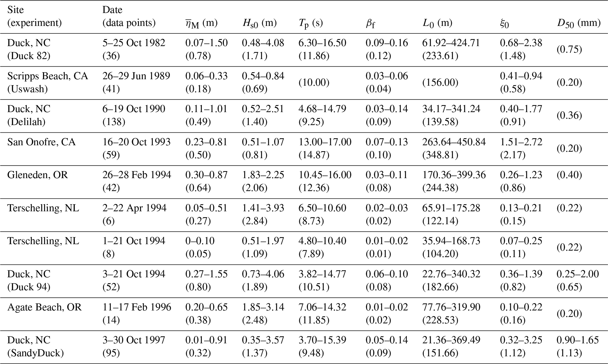
To make setup predictions using a data-driven model, it is necessary to have the input and output data to train it. The input data are related to physical processes that induce the output, wave setup. In this work, we used a dataset meeting these requirements, representing a large variety of beach and wave conditions compiled by Stockdon et al. (2006). The data are freely available, and details on how to access the data can be found in “Code and data availability”. The dataset contains measurements of the following: maximum setup (${\stackrel{\mathrm{‾}}{\mathit{\eta }}}_{\mathrm{M}}$), foreshore beach slope (β_f) – average foreshore slope with respect to still water level ± twice the standard deviation of the continuous water level, and associated offshore wave characteristics (H_s0 – significant wave height, and T_p – peak period) from 10 field experiments on sandy beaches resulting in a total of 491 measurements. Details of the field experiments can be found in Stockdon et al. (2006). From these measurements, additional parameters such as the offshore wavelength ($L_{\mathrm{0}}=g{T_{\mathrm{p}}}^{\mathrm{2}}/\mathrm{2}\mathit{\pi }$) and the Iribarren number (ξ₀) were calculated. Median sediment diameter (D₅₀) data were obtained from reports and papers describing the beaches. Table 1 provides full details of the dataset used in this work, including the location and dates of the experiments and the range and average conditions of the environmental parameters. Figure 1 shows the range for some of the parameters available in the dataset. Beach types vary from highly dissipative ($\stackrel{\mathrm{‾}}{{\mathit{\xi }}_{\mathrm{0}}}=\mathrm{0.11}$ in Terschelling) to fully reflective ($\stackrel{\mathrm{‾}}{{\mathit{\xi }}_{\mathrm{0}}}=\mathrm{2.17}$ in San Onofre) average conditions, with ${\stackrel{\mathrm{‾}}{\mathit{\eta }}}_{\mathrm{M}}$ ranging from 0.00 (Terschelling) to 1.55 m (Duck 94).

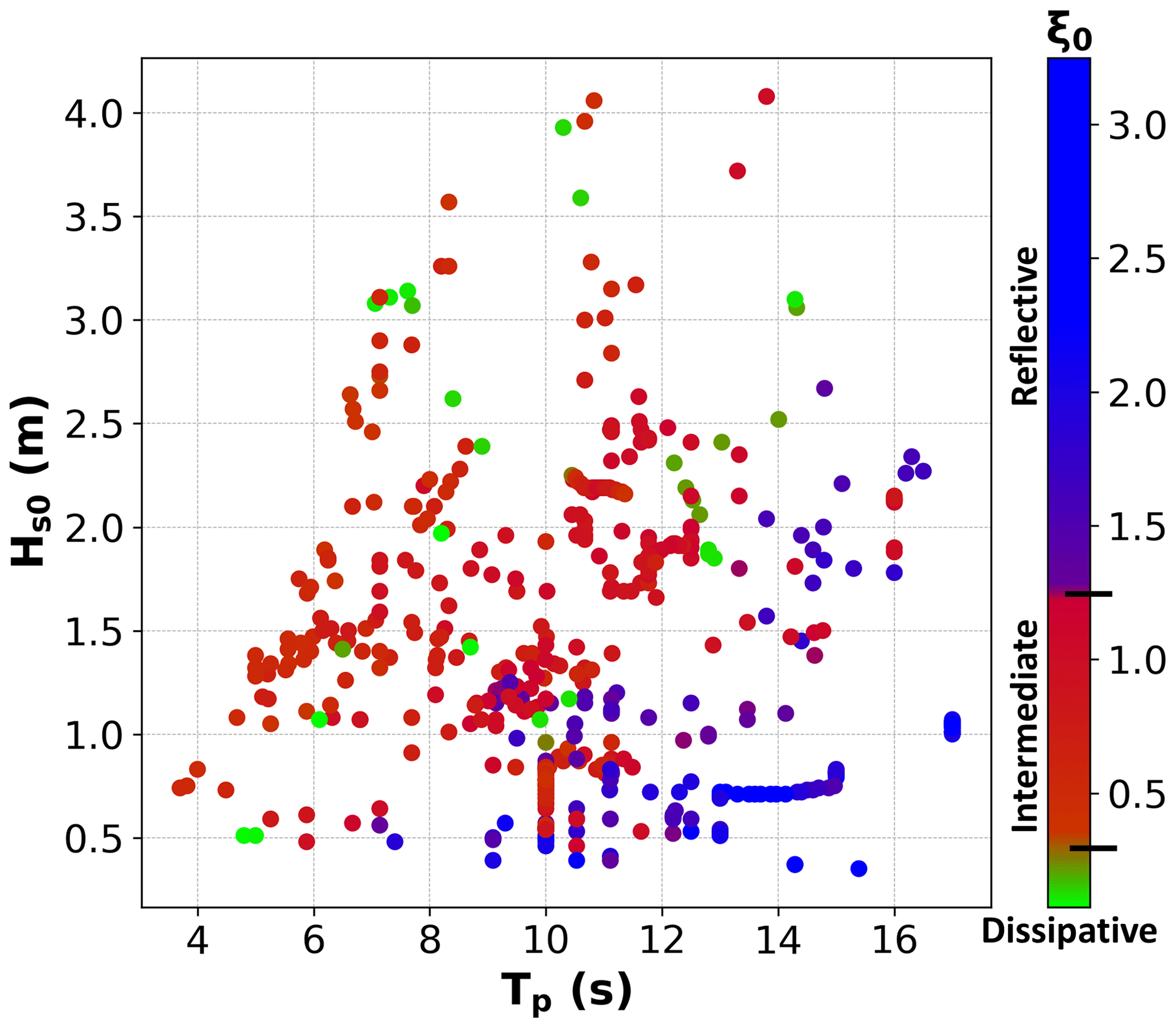
Figure 1 Environmental parameters of the dataset: deep-water wave height (H_s0) versus peak period (T_p). The colours represent the Iribarren number (ξ₀) where values < 0.3 (green) characterize dissipative beaches, values > 1.25 (blue) characterize reflective beaches, and values between both (red) characterize intermediate beaches.

Table 1 Range and average (in brackets) environmental conditions for Stockdon's compiled database (Stockdon et al., 2006). Notice that at times only the average value is available.

2.1.1 Training and testing sets

The target of ML is to use observed data to develop a model able to predict future (unseen) instances. In that sense, the first step is to preprocess the data by normalizing all variables and splitting the dataset into training and testing sets. The training set is used to build and optimize the model, while the testing set is used to quantify the model's performance (i.e. its ability to generalize).

There is no general consensus on which method should be used to split the dataset. In our case, we sought to include the most representative cases from the entire dataset, guaranteeing that the most diverse environmental conditions were well represented in our training set. In addition, the model's aim was not to learn on the largest dataset but to achieve data comprehensiveness with a rather small sample, to later benchmark the model performance against a larger test set. Hence, for this work, we chose the maximum dissimilarity algorithm (MDA; Camus et al., 2011) as the selection routine.

The MDA aims to select points within the series that are the most dissimilar, ensuring the environment's most diverse representation from the original 491 data measurements (Camus et al., 2011). Each data point is a 7-dimensional vector consisting of all the variables in the dataset (${\stackrel{\mathrm{‾}}{\mathit{\eta }}}_{\mathrm{M}}$, H_s0, T_p, β_f, L₀, ξ₀ and D₅₀). During the selection phase, the parameters are normalized between 0 and 1 to receive the same weight in the similarity criterion. The calculation starts by selecting an extreme case. We used the largest wave setup value (${\stackrel{\mathrm{‾}}{\mathit{\eta }}}_{\mathrm{M}}=\mathrm{1.55}$ m) and its related variables as the initial data point. Subsequent points are picked based on the maximum dissimilarity (i.e. largest distance) with respect to the previously selected cases, which no longer participate in the selection. The selection of cases ends when the algorithm reaches the number of points determined by the user, after which the denormalized (i.e. original data) training and test sets are reported.

MDA was applied to select 150 data points (∼30 % of the original dataset), which form the training set. The remaining data (∼70 %) were used as the testing set to evaluate the model's ability to generalize. Besides, having a more extensive testing set ensures a more accurate estimation of model performance, and by avoiding a large training set, we prevent overfitting. The results of MDA selection are shown in Fig. 2.

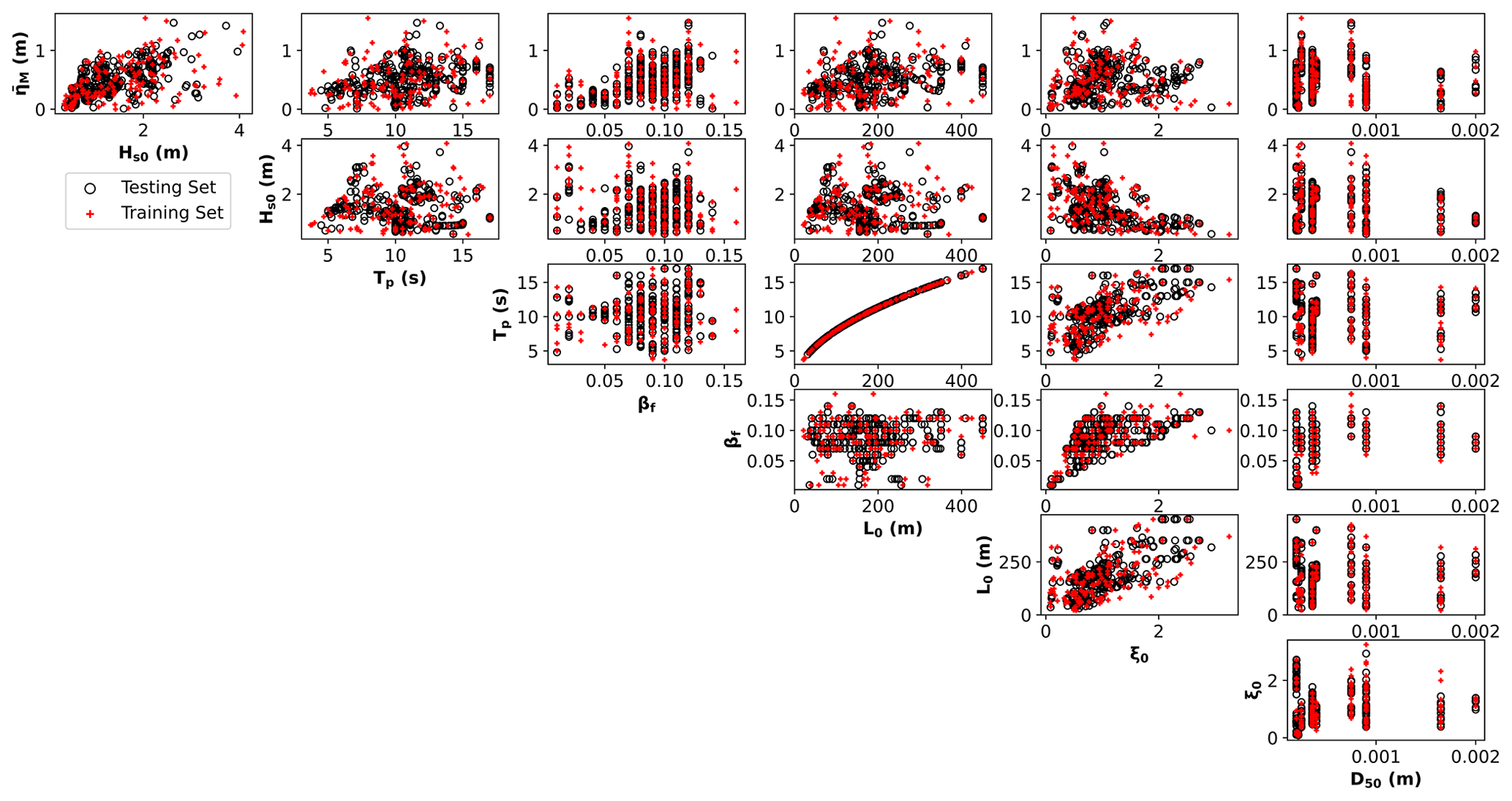
Figure 2 Results of MDA selection and correlation between the variables of the dataset. In red is the training set (∼30 % of the original dataset), and in black is the testing set (∼70 %). Environmental variables considered: maximum wave setup (${\stackrel{\mathrm{‾}}{\mathit{\eta }}}_{\mathrm{M}}$), deep-water significant wave height (H_s0), peak period (T_p), foreshore beach slope (β_f), deep-water wavelength (L₀), Iribarren number (ξ₀), and median sediment diameter (D₅₀).

2.2 Genetic programming

Genetic programming (GP) is an evolutionary computational method for which computers automatically solve a problem without requiring a functional prediction form in advance (Koza and Poli, 2005; Poli et al., 2008). In GP, individuals of a population are computer programs (i.e. equations) of varying size and shape that genetically “breed” (Koza, 1992). The separate elements forming the equations (variables and mathematical operators) represent each individual's chromosomes. Inspired by natural selection and the “survival of the fittest”, GP uses an initial population of equations where the fitter ones (parents) are selected to breed a new generation of offspring (i.e. new equations). At each generation, a new population is created through the application of genetic operations (evolutionary process): reproduction, crossover, and mutation. In the end, the final optimized predictor (within user-defined expression complexity limits) can be represented in a mathematical form. The step-by-step process involved in implementing the GP model is illustrated in Fig. 3 and further explained as follows:

1. [1] Initialization. An initial population of random equations is created by selecting a set of independent variables, mathematical operators, and constant values, which are introduced in agreement with the control parameters of the model set by the user (see Table 2). It is important to highlight that GP does not require non-dimensional (normalized) inputs.

2. [2] Selection. “Tournament” selections between equations are performed in order to decide which equations will evolve in the next generation. Among the selected equations for each tournament, chosen at random from the population, the GP model finds the one that best fits the training data (i.e. lowest fitness function). As the fitness function, we selected the mean absolute error (MAE), which is formulated as

   $$\begin{array}{}\text{(5)}& \mathrm{MAE}={\displaystyle \frac{\mathrm{1}}{n}}\sum _{i=\mathrm{1}}^n|M_i-P_i|,\end{array}$$

   where n is the number of measured values, and M_i and P_i denote measured and predicted values, respectively.

3. [3] Evolution. From the best solutions, a new set of solutions is created through an evolutionary process. Genetic operations are applied to the winner of each tournament at random. Therefore, fitter individuals are more likely to produce new equations than inferior individuals. New equations for the next generation are created by (a) crossover (merging random chromosomes/parts from two tournament winners), (b) mutation (selecting random chromosomes/parts of the tournament winner to change), and (c) reproduction (copy of the tournament winner). A parsimony coefficient is used to penalize long equations, avoiding bloat (longer equations with no significant improvement in fitness). It is used during a tournament to discard from the fitness results the longer equation among two competitors that present identical results.

4. [4] Termination. The execution of the model stops when the termination criterion is reached. The final solution (i.e. equation – encoded as a tree with variables, operators, and coefficients) is the one that reaches the established minimal error (stopping criterion) or the best one at the specific number of generations predetermined by the user.

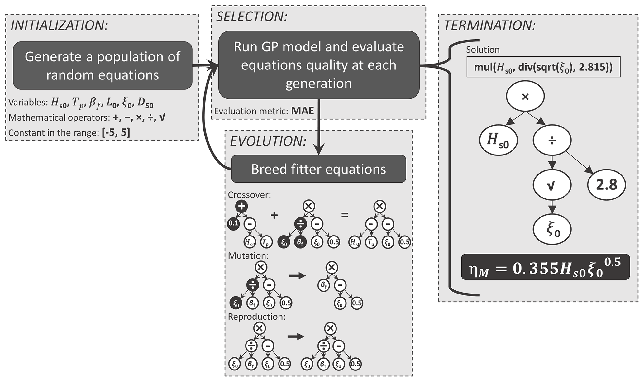
Figure 3 Main loop of the GP model (inspired by Poli et al., 2008). The equations encoded as a tree with variables, operators, and coefficients shown in the evolution framework are examples of genetic operations for the reader's easy visualization. The solution shown in the termination framework is the same one presented later in the “Results” section.

Table 2 Hyperparameter setup of the GPLearn model.

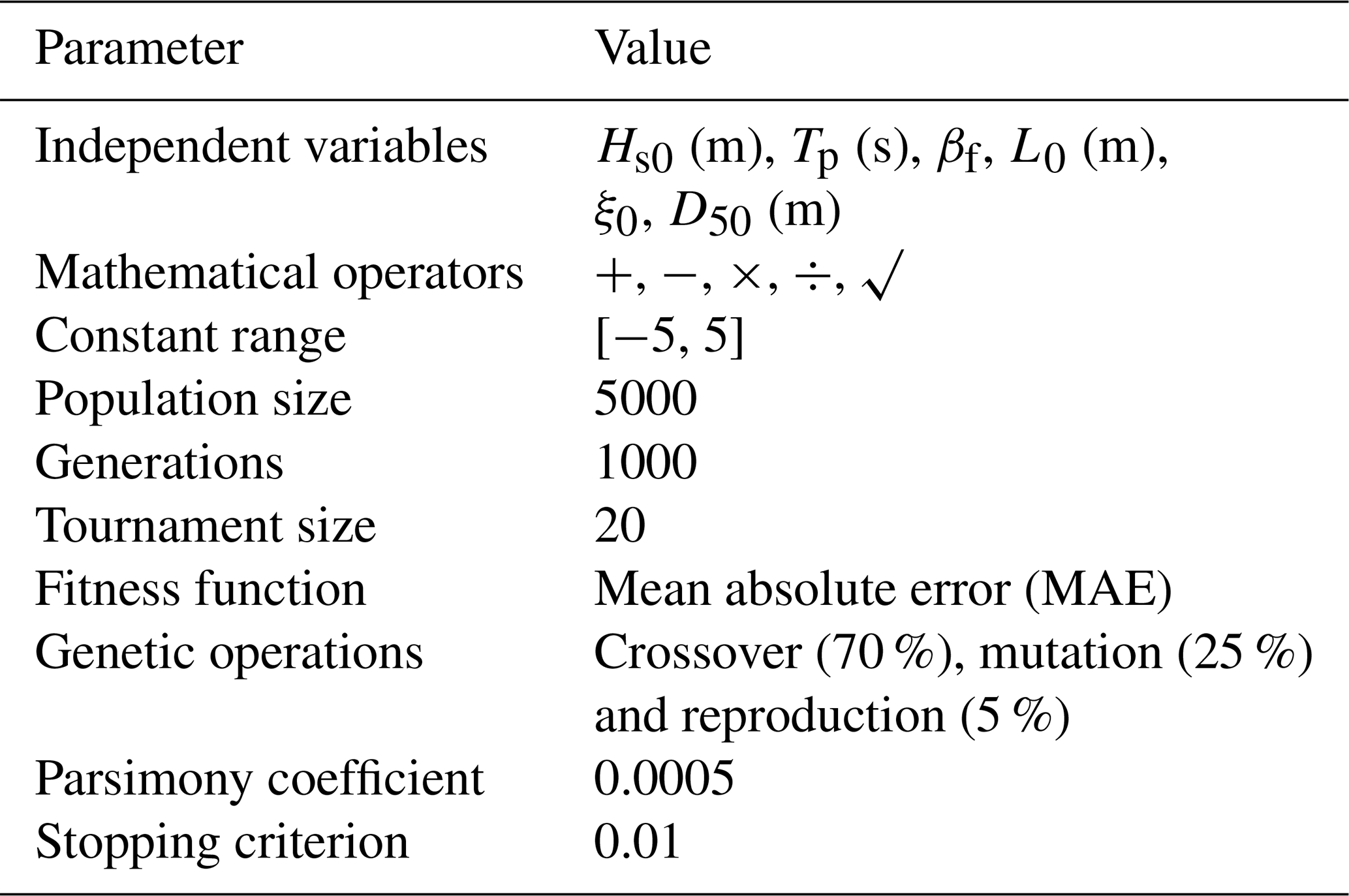
The choice of the values above was driven by extensive testing and sensitivity analyses performed as part of this work. The final model setup for each equation varies slightly. Details of both final codes are available and can be accessed through “Code and data availability”.

In this work, the GP model was built using the GPLearn Python module (Stephens, 2015), a machine learning library extended from scikit-learn (Pedregosa et al., 2011). We have run the model with different setups such as different mathematical operators (addition, subtraction, multiplication, division, square root, power, log, absolute, inverse, sine, cosine, tangent), population sizes (2000–500 000), generations (20–10 000), tournament sizes (10–1000), parsimony coefficients (0.0005–0.01), and genetic operations proportions. Although it is not strictly necessary, we have also run the model using a normalized input. All the runs stopped by reaching the number of chosen generations since we set a very low stopping error criterion. In the end, the best predictors were found through the general model setup presented in Table 2, and minimal or no improvement was achieved with more complicated equations. To select the best predictor, we focused on finding the balance between achieving a low error reduction and high predicting capabilities and obtaining simpler, physically meaningful equations. The code is available, and details on how to access it can be found in “Code and data availability”.

2.3 Model evaluation

The testing dataset was used to evaluate the GP predictor's performance through several statistical parameters, including the square of the correlation coefficient (the square of Pearson's correlation – r² – Eq. 6), coefficient of determination (R² – Eq. 7), modified index of agreement (d₁ – Eq. 8), mean absolute error (MAE – see Eq. 5), and root mean square error (RMSE – Eq. 9), which are defined as follows:

$$\begin{array}{}\text{(6)}& r^{\mathrm{2}}={\displaystyle \frac{\left({\sum }_{i=\mathrm{1}}^n\right(M_i-\stackrel{\mathrm{‾}}{M}\left)\right(P_i-\stackrel{\mathrm{‾}}{P}){)}^{\mathrm{2}}}{{\sum }_{i=\mathrm{1}}^n(M_i-\stackrel{\mathrm{‾}}{M}{)}^{\mathrm{2}}{\sum }_{i=\mathrm{1}}^n(P_i-\stackrel{\mathrm{‾}}{P}{)}^{\mathrm{2}}}}\end{array}$$

$$\begin{array}{}\text{(7)}& R^{\mathrm{2}}=\mathrm{1}-{\displaystyle \frac{{\sum }_{i=\mathrm{1}}^n(M_i-P_i{)}^{\mathrm{2}}}{{\sum }_{i=\mathrm{1}}^n(M_i-\stackrel{\mathrm{‾}}{M}{)}^{\mathrm{2}}}}\end{array}$$

$$\begin{array}{}\text{(8)}& d_{\mathrm{1}}=\mathrm{1}-{\displaystyle \frac{{\sum }_{i=\mathrm{1}}^n|M_i-P_i|}{{\sum }_{i=\mathrm{1}}^n\left(\right|M_i-\stackrel{\mathrm{‾}}{M}|+|P_i-\stackrel{\mathrm{‾}}{M}\left|\right)}}\end{array}$$

$$\begin{array}{}\text{(9)}& \mathrm{RMSE}=\sqrt{{\displaystyle \frac{\mathrm{1}}{n}}\sum _{i=\mathrm{1}}^n(M_i-P_i{)}^{\mathrm{2}}},\end{array}$$

where $\stackrel{\mathrm{‾}}{M}$ and $\stackrel{\mathrm{‾}}{P}$ are the corresponding average values of measured and predicted parameters, respectively.

The values of r² and R² are measures of linear correlation, where r² explains the proportion of variance between two sets of data, and R² is used to evaluate how well the model predicts in comparison to actual measurements (the model's performance). Alternatively, d₁ is also used to evaluate the agreement between predicted and measured values. For further details about d₁ the reader is referred to Willmott (1981) and Willmott et al. (1985). r², R², and d₁ are dimensionless, and values closer to 1 represent better agreements. In contrast, MAE and RMSE measure the errors given by the difference between predicted and measured values; in addition, the second penalizes large errors (bad predictions). Both MAE and RMSE are expressed in the same units of ${\stackrel{\mathrm{‾}}{\mathit{\eta }}}_{\mathrm{M}}$ (m), which means that lower values (closer to 0) indicate more accurate predictions.

Because each metric has its own strengths and limitations, the combination of these five different criteria allowed for a more comprehensive comparison between the model results. Moreover, these same statistical parameters were used to compare the present model with other existing predictors, namely Guza and Thornton (1981), Holman and Sallenger (1985), Yanagishima and Katoh (1990), Hanslow and Nielsen (1993), Stockdon et al. (2006), Ji et al. (2018), and O'Grady et al. (2019).

3 Results

From the multiple equations obtained as an output from the GP model, we selected two predictors of wave setup. A simple predictor is presented in Eq. (10). Alternatively, a more complex but also more accurate predictor, which maintains physical interpretability, is presented in Eq. (11).

$$\begin{array}{}\text{(10)}& {\stackrel{\mathrm{‾}}{\mathit{\eta }}}_{\mathrm{M}}=\mathrm{0.355}{H}_{\mathrm{s}\mathrm{0}}{{\mathit{\xi }}_{\mathrm{0}}}^{\mathrm{0.5}}\end{array}$$

$$\begin{array}{}\text{(11)}& {\stackrel{\mathrm{‾}}{\mathit{\eta }}}_{\mathrm{M}}={\displaystyle \frac{H_{\mathrm{s}\mathrm{0}}}{\mathrm{4.08}}}({\displaystyle \frac{{\mathit{\xi }}_{\mathrm{0}}}{\mathrm{3.25}}}+{\displaystyle \frac{{\mathit{\xi }}_{\mathrm{0}}}{{\mathit{\xi }}_{\mathrm{0}}+\mathrm{0.64}}}+{\displaystyle \frac{{\mathit{\xi }}_{\mathrm{0}}}{\mathrm{1625}{D}_{\mathrm{50}}+{\mathit{\xi }}_{\mathrm{0}}}})\end{array}$$

Here, it is important to highlight that the coefficient 1625 in Eq. (11) is dimensional, with units of per metre. Also, we did simplify the Eq. (11) from the original one, presenting fewer coefficients but with the same output.

Equation (10) stands out for its simplicity. It is also very similar to previous predictors found in the literature (e.g. Holman and Sallenger, 1985; Stockdon et al., 2006; Ji et al., 2018; O'Grady et al., 2019). However, the new models presented here differ from previous equations (except Holman and Sallenger, 1985) by considering wave height, wavelength, and foreshore beach slope combined, in terms of the non-dimensional Iribarren number. Furthermore, the complexity of Eq. (11) is slightly higher because of the additional terms it includes. Similarly to Eq. (10), the first two terms depend only on the wave height and Iribarren number (i.e. they are informed by wave dynamics and beach slope). The third term in Eq. (11) includes D₅₀, measured in metres. Therefore, it requires a dimensional coefficient for the predictor to be dimensionally consistent. As a result, this term contains information on the wave dynamics and beach slope as well as on the sediment size. We remark that this is the first time that grain size is introduced in a wave setup equation.

Figure 4 presents the scatter plots between measured and predicted ${\stackrel{\mathrm{‾}}{\mathit{\eta }}}_{\mathrm{M}}$ obtained from Eqs. (10) and (11). The data shown in the figures are the testing data and the metrics used to evaluate the GP predictors' performance. Although more complex, Eq. (11) represents the best equation in terms of the lowest error when considering the RMSE=0.14 m, in comparison with a RMSE=0.16 m from Eq. (10) (a 12.5 % difference). Nevertheless, note that both equations have the same MAE=0.11 m. Equation (11) also yields higher values of r²=0.70, R²=0.70, and d₁=0.72 as compared to Eq. (10) (r²=0.65, R²=0.64, and d₁=0.71), indicating a better fit of the Eq. (11) with the testing data. Furthermore, Eqs. (10) and (11) performed well on beaches with dissipative (Agate 96) and reflective (San Onofre) conditions. Among all field experiments, Duck 94 (intermediate to reflective with large wave conditions) was the beach that showed less correlation with our models.

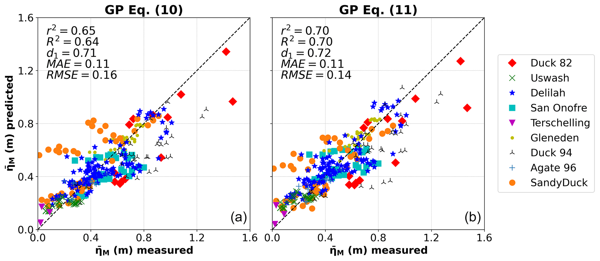
Figure 4 Measured versus predicted maximum wave setup (${\stackrel{\mathrm{‾}}{\mathit{\eta }}}_{\mathrm{M}}$) using the testing data for Eq. (10) (a) and Eq. (11) (b). The metrics used to evaluate the GP predictors' performance are also presented. r² is the square of the correlation coefficient, R² the coefficient of determination, d₁ the modified index of agreement, MAE the mean absolute error, and RMSE the root mean square error. Different markers/colours refer to different field experiments, as referenced in the legend.

A successful predictor should present physical interpretability, but it also must be coherent with the real environment. Therefore, Fig. 5 presents a sensitivity analysis with data in the range measured (in red) and extrapolated (in black) to evaluate the influence of the input variables on ${\stackrel{\mathrm{‾}}{\mathit{\eta }}}_{\mathrm{M}}$. In both models we observe a positive correlation between ${\stackrel{\mathrm{‾}}{\mathit{\eta }}}_{\mathrm{M}}$ and H_s0 and between ${\stackrel{\mathrm{‾}}{\mathit{\eta }}}_{\mathrm{M}}$ and ξ₀. As expected, the linear relationship between ${\stackrel{\mathrm{‾}}{\mathit{\eta }}}_{\mathrm{M}}$ and H_s0 means that larger waves produce greater setups. Regarding Iribarren number, ${\stackrel{\mathrm{‾}}{\mathit{\eta }}}_{\mathrm{M}}$ is proportional to the square root of ξ₀ in Eq. (10), and a similar non-linear relationship appears in Eq. (11). In this case, greater setups are likely to occur for reflective beach conditions (higher ξ₀). However, the rate of increase in setup decreases with higher Iribarren numbers in both cases. On the other hand, D₅₀ (which only appears in Eq. 11) is negatively correlated with ${\stackrel{\mathrm{‾}}{\mathit{\eta }}}_{\mathrm{M}}$, meaning that greater setups are expected to occur on beaches with smaller sediment diameters. The variation in setup with D₅₀ appears to be of lower magnitude in comparison with H_s0 and ξ₀. However, with increasing H_s0, the sensitivity of ${\stackrel{\mathrm{‾}}{\mathit{\eta }}}_{\mathrm{M}}$ to the median grain size (D₅₀) increases. This is not the case for ξ₀. On the contrary, there is a slight decrease in the sensitivity of ${\stackrel{\mathrm{‾}}{\mathit{\eta }}}_{\mathrm{M}}$ as a function of D₅₀ with larger ξ₀ values. Here, we have expanded the predictor's use beyond the range of the measurements that comprise the dataset, to test its general behaviour and stability, showing that the predictors work sensibly also beyond the range of the available measurements. Smaller values of H_s0 and ξ₀ never result in negative ${\stackrel{\mathrm{‾}}{\mathit{\eta }}}_{\mathrm{M}}$ values, and the observed trends continue beyond the training range.

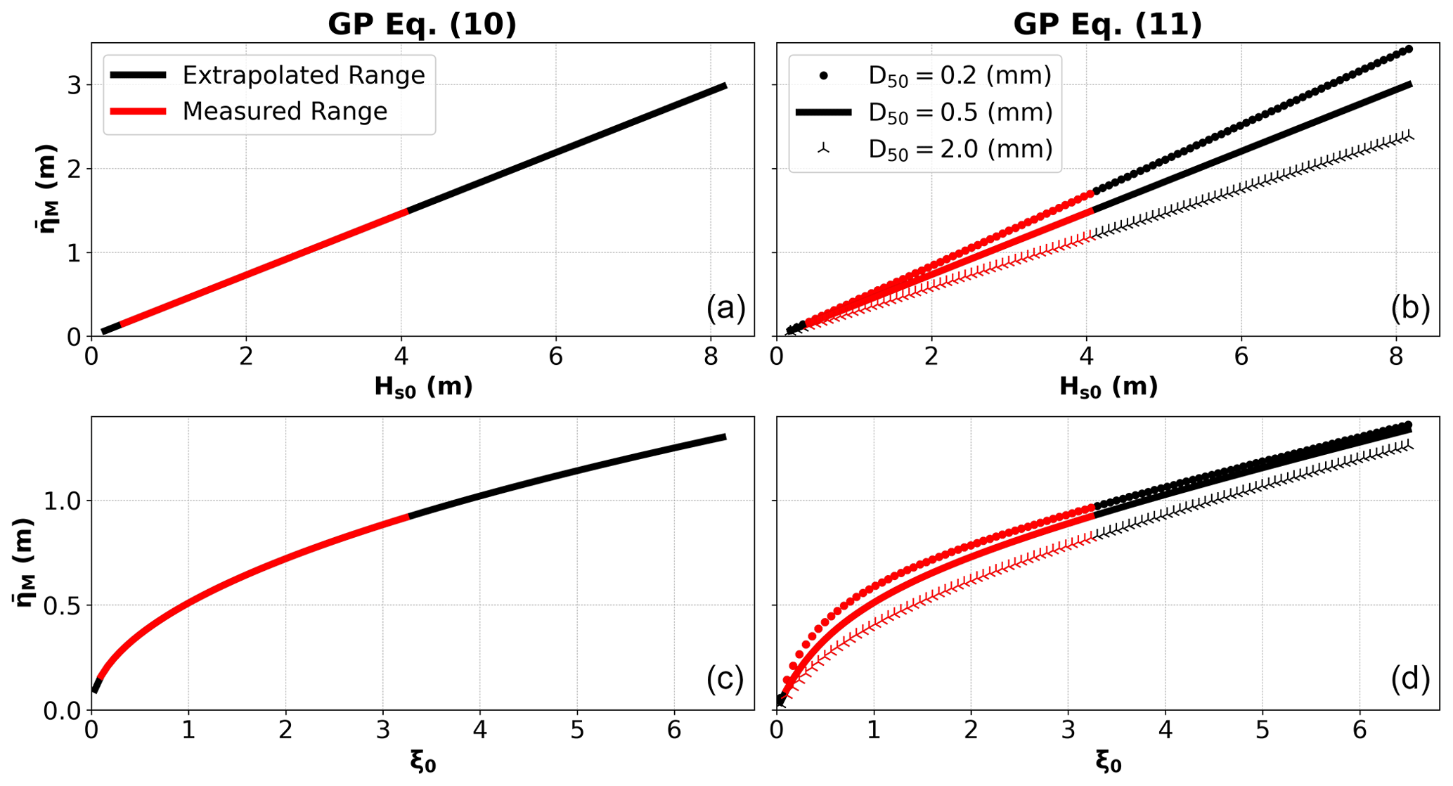
Figure 5 General behaviour of the maximum wave setup (${\stackrel{\mathrm{‾}}{\mathit{\eta }}}_{\mathrm{M}}$) predictors presented in Eq. (10) (a, c) and Eq. (11) (b, d), as a function of deep-water significant wave height (H_s0), Iribarren number (ξ₀), and median sediment diameter (D₅₀). D₅₀ is represented by its minimum (0.2 mm), mean (0.5 mm), and maximum (2.0 mm) values in the dataset. Data within the measured range are depicted in red. Black represents an extrapolated range for H_s0 and ξ₀. Note the different Y and X axis ranges for each graph.

Using the entire dataset (training + testing), we also compared the results of Eqs. (10) and (11) with the most widely known predictors in the literature. Table 3 and Fig. 6 show the performance of nine distinct empirical equations, including the ones presented in this work, in determining maximum wave setup. Equations (10) and (11) show a good agreement with the measured dataset, with less scatter (especially Eq. 11) if compared with the others. Overall, our ML-driven approach achieved better results with Eq. (11) outperforming all other predictors. Similarly, Eq. (10) exhibits good results, the same ones as the equation of Ji et al. (2018), which also performs well on dissipative and reflective beach conditions. In comparison, the Stockdon et al. (2006) formulation presents lower metrics results. Correlation and agreement results showed by the equation in O'Grady et al. (2019) are also close to that of Ji et al. (2018) and Eq. (10) in this work. In contrast, their model prediction is worse. Finally, the predictors of Holman and Sallenger (1985) and Hanslow and Nielsen (1993) produce more scatter and tend to overestimate the results, while the predictors of Guza and Thornton (1981) and Yanagishima and Katoh (1990) largely underestimate the setup values. This results in very low coefficients of determination, meaning that their predictions match poorly with observations. Here, it is worth pointing out that models with the same correlation coefficient, e.g. Holman and Sallenger (1985) and Stockdon et al. (2006), present similar patterns. However, the coefficient of determination appears to better describe the accuracy of the model predictions. Considering the coefficient of determination, the equation of Stockdon et al. (2006) performs better than that of Holman and Sallenger (1985).

Guza and Thornton (1981)Holman and Sallenger (1985)Yanagishima and Katoh (1990)Hanslow and Nielsen (1993)Stockdon et al. (2006)Ji et al. (2018)O'Grady et al. (2019)

Table 3 Statistical metrics of predictors' performance using measured data from Stockdon et al. (2006). We assumed $H_{\mathrm{rms}\mathrm{0}}=H_{\mathrm{s}\mathrm{0}}/{\mathrm{2}}^{\mathrm{0.5}}$, following Rayleigh distribution in deep water. ${\stackrel{\mathrm{‾}}{\mathit{\eta }}}_{\mathrm{M}}$ is maximum wave setup, r² the square of the correlation coefficient, R² the coefficient of determination, d₁ the modified index of agreement, MAE the mean absolute error, and RMSE the root mean square error.

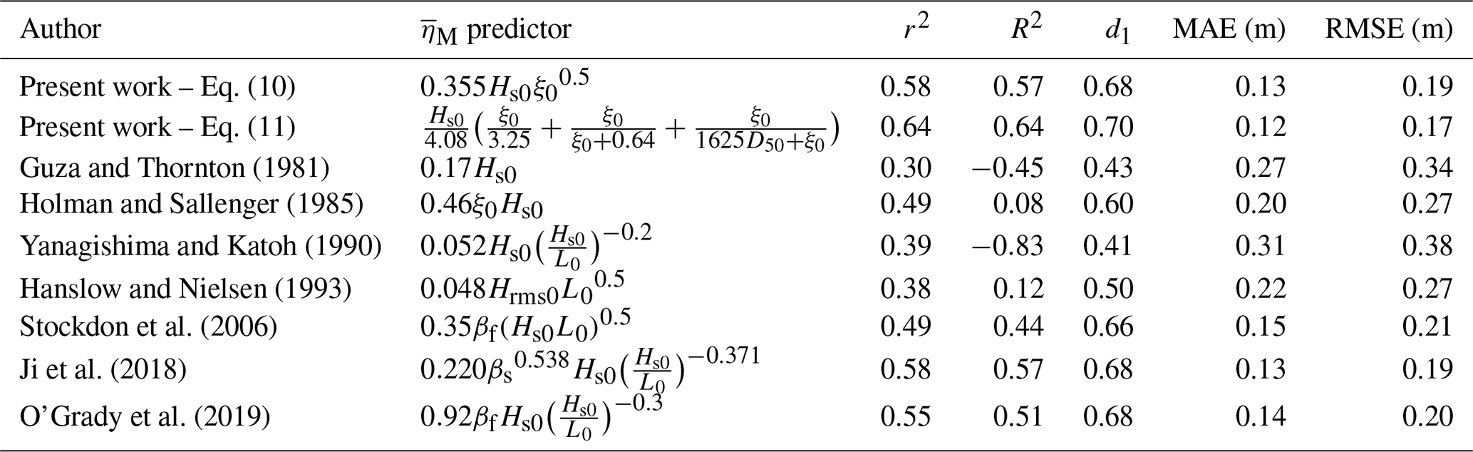
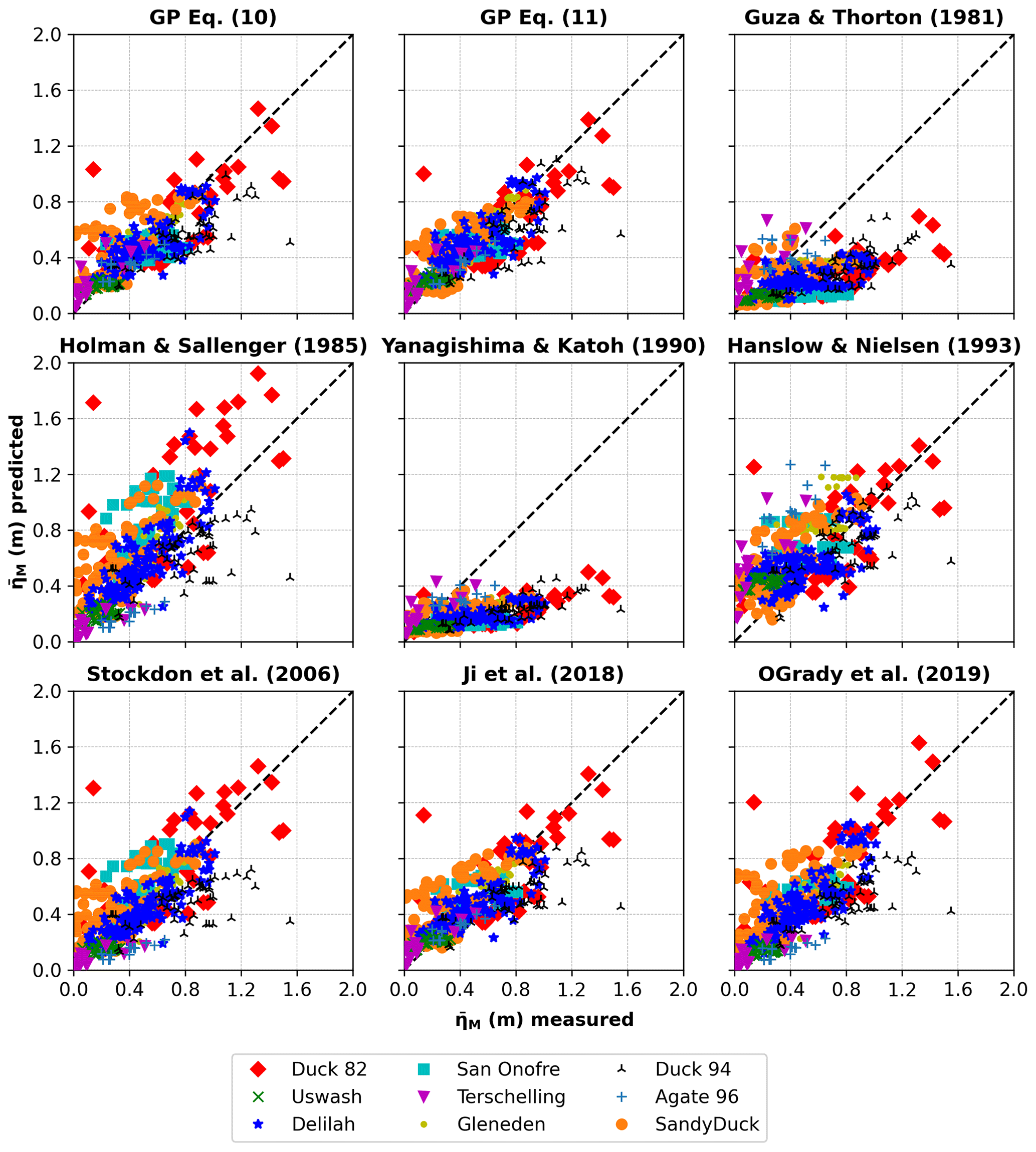
Figure 6 Measured versus predicted maximum wave setup (${\stackrel{\mathrm{‾}}{\mathit{\eta }}}_{\mathrm{M}}$) using the entire dataset (training + testing) for nine distinct empirical equations, including the ones presented in this work. Different markers/colours denote different field experiments, as referenced in the legend.

4 Discussion

We have presented two predictors that demonstrate the predictive capability of genetic programming. The results show that the novel GP predictor (Eq. 11) outperforms existing formulas by presenting a fitter equation for the entire dataset compiled by Stockdon et al. (2006). Likewise, Eq. (10) also provides promising results. Additionally, unlike most previous predictors, they also present a good fit for both dissipative (Agate 96) and reflective (San Onofre) beach conditions. Although the main advantage of the GP model is the possibility of fully exploring multiple equation forms from different model parameters trying to find a more accurate variable combination during evolution, the final selection of the proposed solution remains subjective. This last step requires the user to have knowledge of the specific topic so that the expression chosen is dimensionally and physically correct. Generally, as the complexity of the solutions increases, the error decreases. Therefore, more complex predictors usually fit the training dataset better than simpler ones. However, they may become too specific for the training dataset; thus, they may lose generalization power (due to overfitting) when applied to different datasets (Tinoco et al., 2015; Passarella et al., 2018). As a result, the proposed solutions should ideally be simple, be easy-to-use and to interpret, and have a physical meaning.

The variables (H_s0, β_f, L₀) in the two obtained predictors are the same as those used in previous published works (Holman and Sallenger, 1985; Stockdon et al., 2006; Ji et al., 2018; O'Grady et al., 2019) but with a different arrangement. The result is in agreement with Longuet-Higgins and Stewart (1964), who stated the cross-shore gradient of radiation stress is principally controlled by the wave height. Additionally, in line with O'Grady et al. (2019), we found the wave setup predictor is best parameterized with the inclusion of wave steepness and beach slope (through the Iribarren number) along with the wave height. Although playing a limited role, sediment diameter also appears in Eq. (11) improving the performance of the predictor by establishing a non-linear, inversely proportional relationship with the maximum wave setup.

Most wave setup studies (e.g. Guza and Thornton, 1981; King et al., 1990) present the offshore wave height as the primary contributing factor to wave setup, since it dictates the energy available for the production of setup. Nevertheless, the wave setup is not simply a result of incident waves but is also induced by the shape of the beach profile. Studies have shown that detailed knowledge of the beach morphology can help improve the predictor (Stephens et al., 2011; O'Grady et al., 2019; Gomes da Silva et al., 2020). However, there is no consensus on which region to use to estimate the beach slope. Some works include only the foreshore beach slope (Holman and Sallenger, 1985; Hanslow and Nielsen, 1993; Stockdon et al., 2006; O'Grady et al., 2019) into the predictor, and some use the average surf zone beach slope (Bowen et al., 1968; Raubenheimer et al., 2001; Stephens et al., 2011; Gomes da Silva et al., 2020). Despite being difficult to quantify, the role of beach slope is essential in incorporating the effect of the cross-shore beach profile in estimating wave setup. The presence of sediment diameter in Eq. (11) also needs careful further consideration. As in Poate et al. (2016) and Power et al. (2019), who stated the importance of grain size in runup parameterization, its inclusion also improves wave setup prediction. This second-order effect could be tentatively related to beach permeability, which increases with sediment size and results in a lower setup. However, the limited amount of sediment diameter data may not be entirely appropriate to claim such finding. An avenue for future research includes the validation of the GP predictors (Eqs. 10 and 11) by applying them to datasets not included in the training. This will further assess the predictive capability of the new formulas and the importance of each term in the equations.

More importantly, the novel inclusion of D₅₀ as a second-order effect may indicate that we still have very limited information to describe an entire beach. Other examples of second-order effects are not considering the presence of multiple bar systems or even incorporating wave direction. After over 50 years of research, wave setup prediction still presents a number of issues to be solved in future works which can enhance parametric predictors based on environmental variables. These also include the influence of beach permeability (Longuet-Higgins, 1983; Nielsen, 1988, 1989) and tide (Holman and Sallenger, 1985; Raubenheimer et al., 2001; Stockdon et al., 2006) as second-order processes subject to discussion. More recently, works from Guérin et al. (2018) and Martins et al. (2022) investigated the role of the wave-induced nearshore circulation processes (bottom stress, vertical mixing, and vertical and horizontal advection), resulting in an improved wave setup prediction across the surf zone. The contribution of these parameters can be even larger on steeper beach slopes (Martins et al., 2022).

In the field, different methodologies have been used to measure wave setup. Applied equipment includes resistance wire runup meters (Guza and Thornton, 1981), manometer tubes (Nielsen, 1988), pressure transducers/sensors (King et al., 1990; Lentz and Raubenheimer, 1999; Raubenheimer et al., 2001), sonar altimeters (Lentz and Raubenheimer, 1999; Raubenheimer et al., 2001), and video cameras (Holman and Sallenger, 1985). O'Grady et al. (2019) suggested that around ∼46 % of the setup variance is possibly explained by measurement errors or related to critical processes that could not be translated into simple predictors yet. Since the surf and swash zones are a highly dynamic environment, the bathymetry is rapidly evolving and changes are difficult to predict. In an attempt to overcome this problem, Ji et al. (2018) used a wave–current numerical model to generate setup data for idealized beach conditions. Even with such approach, there is still a significant scatter around the wave setup predictor. Furthermore, Martins et al. (2022) suggest that it might be difficult to differentiate between swash and wave motions near the shoreline in the field, particularly for steeper foreshores. The considerable influence of the swash circulation within a cusp field during the Duck 94 experiment described by Stockdon et al. (2006) could be an explanation for the lowest correlation of the measured data with the results of GP predictors. In essence, measuring and accounting for all the effects and processes that may be important for wave setup remains an arduous challenge.

5 Conclusions

In this work, we proposed two new empirical equations for the maximum wave setup using data compiled by Stockdon et al. (2006) to feed an evolutionary-based genetic programming model. A simple, yet accurate, predictor and a more complex but fitter predictor, which maintains physical interpretability, were tested and evaluated against other seven widely known empirical equations for maximum wave setup. The results of both GP-based predictors emphasized similarities with previous ones and incorporated new dependencies. Compared with previous predictors, the new ones (particularly Eq. 11) demonstrate an improvement in prediction performance and goodness of fit for a wide range of environmental conditions, including both dissipative and reflective beaches. The novel predictors are simple, can be easily used in practical applications, and open up new paths for future wave setup research.

So far, only a few studies have addressed wave setup predictions, and all past predictors present significant scatter around the data. All predictors share similarities in their structure, possibly indicating that limits in predictability are related to the use of oversimplified variables, H_s0, T_p, β_f, and D₅₀, that do not fully capture the complexity of surf zone processes. The use of additional parameters (e.g. to better describe the surf zone seabed profile and nearshore circulation processes) appears necessary to more accurately describe wave setup in a natural environment. As additional data become available and better algorithms are developed, more accurate predictors will be generated. Data-driven approaches are able to extract patterns from samples resulting in higher performance and more cost-effective predictors. Although we still need to deal with data scarcity and measurement uncertainties, our results reveal that the genetic programming model is competent in data generalization. Being a data-driven technique, it will be more accurate as additional high-quality data become available.

Understanding and predicting nearshore processes is vital to protect coastal resources and people living near the shore. The results of this work can contribute to improving the predictability of wave setup, a key factor in coastal flooding. Additionally, we also seek to stimulate further discussion about the use of machine learning as a powerful data analysis tool and the possibility of its use to improve coastal sciences/management.