A methodological framework for the evaluation of short-range flash-flood hydrometeorological forecasts at the event scale

This paper presents a methodological framework designed for the event-based evaluation of short-range hydrometeorological ensemble forecasts, in the specific context of an intense flash-flood event characterized by high spatiotemporal variability. The proposed evaluation adopts the point of view of end users in charge of the organization of evacuations and rescue operations at a regional scale. Therefore, the local exceedance of discharge thresholds should be anticipated in time and accurately localized. A step-by-step approach is proposed, including first an evaluation of the rainfall forecasts. This first step helps us to define appropriate spatial and temporal scales for the evaluation of flood forecasts. The anticipation of the flood rising limb (discharge thresholds) is then analyzed at a large number of ungauged sub-catchments using simulated flows and zero-future rainfall forecasts as references. Based on this second step, several gauged sub-catchments are selected, at which a detailed evaluation of the forecast hydrographs is finally achieved.

This methodology is tested and illustrated for the October 2018 flash flood which affected part of the Aude River basin (southeastern France). Three ensemble rainfall nowcasting research products recently proposed by Météo-France are evaluated and compared. The results show that, provided that the larger ensemble percentiles are considered (75th percentile for instance), these products correctly retrieve the area where the larger rainfall accumulations were observed but have a tendency to overestimate its spatial extent. The hydrological evaluation indicates that the discharge threshold exceedances are better localized and anticipated if compared to a naive zero-future rainfall scenario but at the price of a significant increase in false alarms. Some differences in the performances between the three ensemble rainfall forecast products are also identified.

Finally, even if the evaluation of ensemble hydrometeorological forecasts based on a low number of documented flood events remains challenging due to the limited statistical representation of the available data, the evaluation framework proposed herein should contribute to draw first conclusions about the usefulness of newly developed rainfall forecast ensembles for flash-flood forecasting purpose and about their limits and possible improvements.

1 Introduction

Flash floods contribute in a significant proportion to flood-related damage and fatalities in Europe, particularly in the Mediterranean countries (Barredo, 2006; Llasat et al., 2010, 2013; Petrucci et al., 2019). As an illustration, over the period 1989–2018, four of the eight most damaging floods in France were flash floods, each having caused insurance losses that exceeded EUR 500 million according to the French Central Reinsurance Fund (CCR, 2020). These floods are characterized by fast dynamics and high specific discharges (Gaume et al., 2009; Marchi et al., 2010), which largely explain their destructive power. They generally result from heavy precipitation events, typically exceeding hundreds of millimeters of rainfall totals in less than 6 h, falling over river basins of less than 1000 km² of drainage area. They are also characterized by a high spatiotemporal variability and limited predictability (Georgakakos, 1986; Borga et al., 2008). Improving the capacity of flood monitoring and forecasting systems to anticipate such events is a key factor to limit their impacts and improve flood risk management. Although several operational flash-flood monitoring services based on weather radar rainfall have already been implemented worldwide (Price et al., 2012; Clark et al., 2014; de Saint-Aubin et al., 2016; Javelle et al., 2016; Gourley et al., 2017; Park et al., 2019), these systems can only offer limited anticipation due to the short response times of the affected catchments. The integration of short-range, high-resolution rainfall forecasts in flash-flood monitoring services is required to increase anticipation times beyond current levels (Collier, 2007; Hapuarachchi et al., 2011; Zanchetta and Coulibaly, 2020).

Weather forecasting systems that are well suited to capture heavy precipitation events have been developed in the last decade with the emergence of high-resolution and convection-permitting numerical weather prediction (NWP) models (Clark et al., 2016). The spatial and temporal resolutions of such models (typically 1 km and 1 min) are more relevant to the scales of the (semi-)distributed hydrological models that are commonly used in flash-flood monitoring and forecasting systems. Convection-permitting NWP models may also be combined with radar measurements through assimilation and/or blending techniques to obtain improved and seamless short-range rainfall forecasts (Davolio et al., 2017; Poletti et al., 2019; Lagasio et al., 2019). Despite these advances, the use of high-resolution rainfall forecasts to issue flash-flood warnings still faces numerous challenges mainly due to the uncertainties in the temporal distribution and the spatial location of the high rainfall accumulation cells over small areas (Silvestro et al., 2011; Addor et al., 2011; Vincendon et al., 2011; Hally et al., 2015; Clark et al., 2016; Armon et al., 2020; Furnari et al., 2020). Accurate forecasts and a reliable representation of forecast uncertainties are thus necessary to provide useful flash-flood warnings based on outputs of NWP models. The question of quantifying uncertainties in hydrometeorological forecasting systems has been increasingly addressed through ensemble forecasting approaches (e.g., Valdez et al., 2022; Bellier et al., 2021; Thiboult et al., 2017). Several ensemble flash-flood forecasting chains have been proposed in the literature, involving either convection-permitting NWP models for early warnings (Silvestro et al., 2011; Addor et al., 2011; Vié et al., 2012; Alfieri and Thielen, 2012; Davolio et al., 2013, 2015; Hally et al., 2015; Nuissier et al., 2016; Amengual et al., 2017; Sayama et al., 2020; Amengual et al., 2021) or radar advection approaches and/or radar data assimilation in NWP models for very short-range forecasting (Berenguer et al., 2011; Vincendon et al., 2011; Silvestro and Rebora, 2012; Davolio et al., 2017; Poletti et al., 2019; Lagasio et al., 2019).

New approaches to flash-flood forecasting need to be appropriately evaluated and cannot rely only on the evaluation of the high-resolution rainfall forecasts used as input. In one sense, flood forecasting verification can be seen as a form of fuzzy verification of rainfall forecasts (Ebert, 2008; Roberts and Lean, 2008), accounting for the averaging effect and the nonlinearity of the rainfall–runoff process and also for the positions of the watershed limits. Flood forecast evaluation is generally based on long time series of observed and forecast data. However, in the case of flash-flood forecast evaluation, working on long time series is often not possible. Firstly, high-resolution ensemble rainfall forecasts from convection-permitting NWP models are rarely available for long periods of re-forecasts. This is due to the fast evolution of input data (type, availability) and the frequent updates brought to the NWP models or the data assimilation approaches (Anderson et al., 2019). Secondly, because of the limited frequency of occurrence of heavy precipitation events triggering flash floods, the datasets available for evaluation often include only a few significant flood events, which highly limits the possibility of satisfying the typical requirements for a statistically robust evaluation of hydrological forecasts (Addor et al., 2011; Davolio et al., 2013). Therefore, the evaluation of experimental flash-flood forecasting systems based on newly developed rainfall forecast products often has to begin with event-based evaluations. Even if such preliminary evaluations cannot provide a complete picture of the performance of the forecasting systems, they may bring useful information about their value for some rare, high-impact flood events, and they can help to decide if the tested systems are worth running in real time for preoperational evaluations at larger space and timescales. They can also be useful communication tools to exchange and get feedback from the end users of forecasts in the system design phase (Dasgupta et al., 2023). Finally, event-based and statistical evaluations of flood forecast systems should probably not be considered as opposite but rather complementary approaches (ECMWF, 2022).

Event-based evaluations generally rely on the visual inspection of forecasts against observed hydrographs or on the assessment of the anticipation of exceedances over predefined discharge thresholds at a few gauged outlets, where the main hydrological responses to the high rainfall accumulations were observed during the event (Vincendon et al., 2011; Vié et al., 2012; Davolio et al., 2013; Hally et al., 2015; Nuissier et al., 2016; Amengual et al., 2017; Lagasio et al., 2019; Sayama et al., 2020). When different forecast runs are available for the same event and along its duration (e.g., short-range forecasts generated by NWP models from different forecast initialization cycles) and/or when different basins are affected by the same event, statistical scores and frequency analyses, such as the RMSE, the CRPS (continuous ranked probability score), contingency tables or receiver operating characteristic (ROC) curves, may also be used to provide a synthetic evaluation of the performance of the forecasts for the event being evaluated (Davolio et al., 2017; Poletti et al., 2019; Sayama et al., 2020). Although widely used in the scientific literature and in post-event reports, these evaluation frameworks raise several methodological questions: (i) the focus on one event or a few typical severe events may generate an event-specific evaluation which might not be reproducible across different events or might not be statistically representative of forecast performance for other future events; (ii) scores that offer a synthesis of performance over spatial and temporal scales might conceal the internal (in space and in time) variability in forecast performance (over different forecast initialization times and along lead times); and (iii) forecast evaluations that focus on gauged outlets that display the main hydrological responses to rainfall only offer a partial view of the forecasting system's performance, notably when impacts are also observed at ungauged sites and/or when significant spatial shifts exist between observed and forecast rainfalls. Therefore, the evaluation of short-range flash-flood forecasts at the event scale requires the consideration of specific forecast quality attributes evaluated at gauged sites (where observations are available) but also a more regional-scale evaluation at ungauged sites in order to achieve a more robust evaluation of forecast performance. Several authors already pointed out the interest of providing such regional-scale hydrological evaluations (Silvestro and Rebora, 2012; Davolio et al., 2015; Anderson et al., 2019; Sayama et al., 2020).

In this paper, an evaluation of three new ensemble rainfall forecast products is presented in the perspective of their use for flash-flood forecasting. The evaluated products have been specifically developed by the French meteorological service (Météo-France) to generate short-range rainfall forecasts (1 to 6 h of lead time) that can potentially better capture Mediterranean heavy precipitation events. The products comprise the French AROME-EPS reference ensemble forecast (Bouttier et al., 2012; Raynaud and Bouttier, 2016) and two experimental products merging AROME-EPS and another convection-permitting NWP model, AROME-NWC (Auger et al., 2015), with the optional incorporation of spatial perturbations as post-processing (Vincendon et al., 2011). Since the two experimental products have been released only for the autumn 2018 period in France, the evaluation can only be based on one significant flash-flood event, i.e., the heavy flood that occurred in the Aude River basin on 15 October 2018. Therefore, a new framework is proposed for the evaluation of flash-flood hydrometeorological ensemble forecasts at the event scale. This approach is based on the combination and adaptation of well-known evaluation metrics, with the objective to provide a detailed and as meaningful as possible analysis of the considered event. The evaluation is mainly focused on the capacity of the hydrometeorological forecasts to anticipate the exceedance of predefined discharge thresholds and to accurately localize the affected streams within the region of interest. These are two essential qualities of hydrometeorological forecasts that are needed to plan rescue operations in real time. The forecast-based financing approach developed for humanitarian actions adopts a similar pragmatic approach but with the aim to release funding and trigger short-term actions in disaster-prone areas worldwide (Coughlan de Perez et al., 2015). Others methods with a specific interest for operational considerations have also been recently proposed for the case of deterministic forecasts (Lovat et al., 2022).

In the following, Sect. 2 presents the step-by-step evaluation framework proposed for the event-scale evaluation of ensemble forecasts. Section 3 presents the case study, the data and models used to produce discharge forecasts. In Sect. 4, the obtained results are presented and evaluated. Section 5 discusses the main outcomes, while Sect. 6 summarizes the conclusions and draws the perspectives of this study.

2 Methodology for an event-scale evaluation of hydrometeorological ensemble forecasts

The proposed evaluation framework aims at determining if the magnitude of the floods generated by heavy precipitation events can be correctly anticipated based on ensemble rainfall forecasting products. It is considered that such products might not perfectly capture the complex spatial and temporal patterns of the observed rainfall, although they might still be useful to inform flood risk decision-making. More precisely, the question of anticipating high discharges that might exceed predefined discharge thresholds is addressed. The evaluation should not focus only on selected river sections but offer a comprehensive view of anticipation capacities for the whole river network, including ungauged rivers.

Another challenge of the event-scale evaluation is to select a limited number of aggregated criteria that help us to draw sound conclusions owing to the possible high spatial and temporal variability in rainfall and runoff values and of model performance, as well as to the many possible combinations of time steps, forecast lead times and locations along the river network that need to be considered in the evaluation. For this reason, a step-by-step approach is proposed (Fig. 1). It is first based on an initial assessment of the rainfall forecasts, with a focus on the time and space windows of observed or forecast high rainfall accumulations. Then, a geographical analysis of the anticipation capacities of the ensemble flood forecasts is performed at a large number of ungauged outlets, focusing on the most critical phase of the floods (hydrograph rising limbs). Based on this second step, a detailed evaluation of the performance of the flood forecasts is conducted at some selected representative catchment outlets. These different steps are described below.

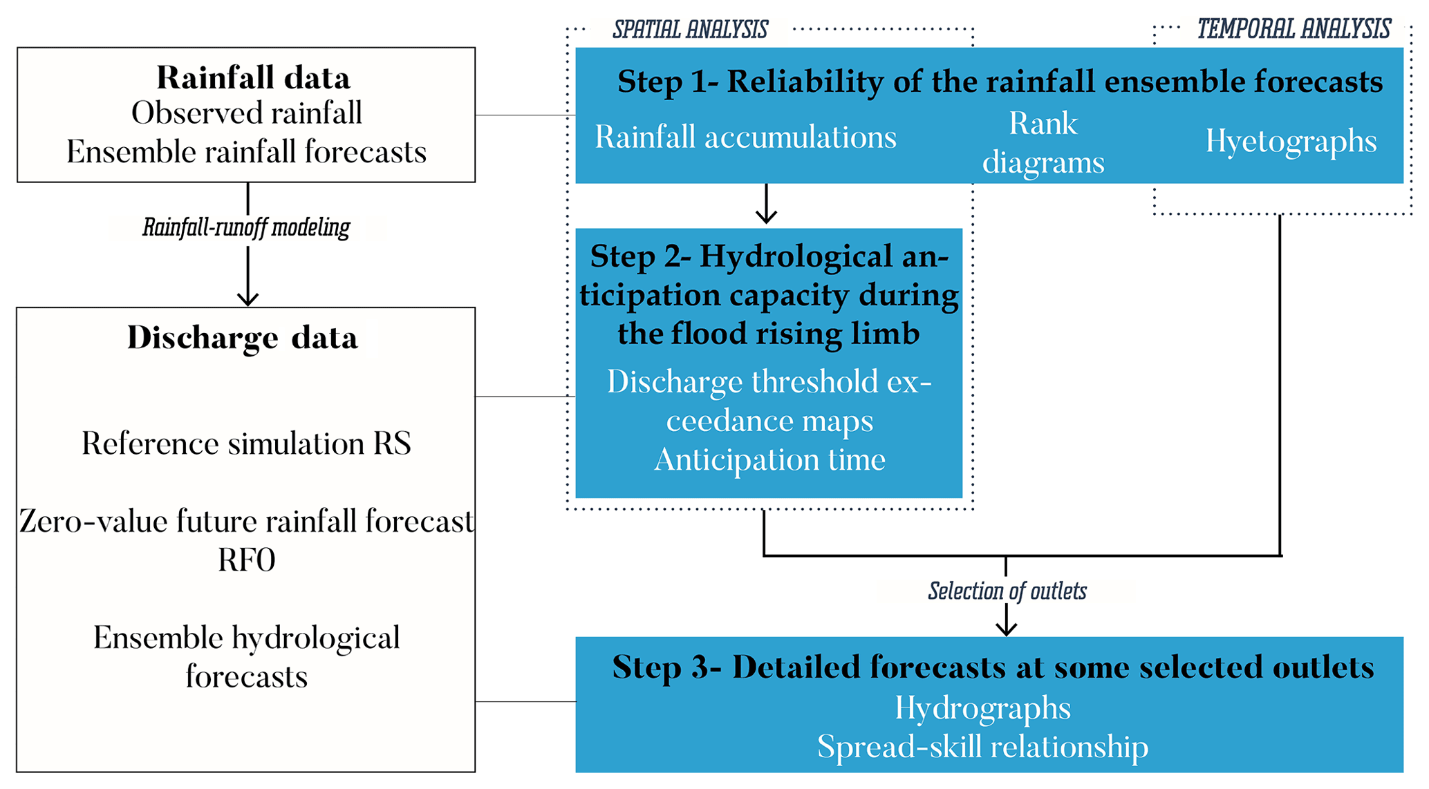
Figure 1 Overall principle of the proposed evaluation framework with its three steps of evaluation along the hydrometeorological forecasting chain.

2.1 Step 1: reliability of the rainfall ensemble forecasts

The twofold objective of this initial phase is to analyze the quality of the rainfall forecasts and to define the relevant spatial and temporal scales to be used in the subsequent analyses. Three different aspects are considered for a comparison of observed and forecast rainfall values.

• The hyetographs of the average rainfall intensities over the studied area are first plotted for each rainfall ensemble product and the different forecast lead times. They are used to assess if, on average, the time sequence and the magnitude of the rainfall intensities are well captured by the products. A reduced time window, where significant intensities are forecast or measured, is selected for the next steps of the analysis. This time window is hereafter called “hydrological focus time” (HFT).

• Maps of the sum of forecast and observed hourly rainfall amounts during the HFT are then generated to assess if the areas where high rainfall accumulations were predicted and actually occurred coincide. One map is produced per forecast product, forecast lead time and ensemble percentile. These maps compare the spatial distribution of accumulated rainfalls from the aggregation of all forecast runs that were delivered during the event. It is thus the rainfall totals that are first evaluated. These maps also help us to delineate the areas affected by high totals of measured or forecast rainfalls. The next evaluation steps will focus on these areas, which are hereafter designated as “hydrological focus area” (HFA).

• Classical rank diagrams (Talagrand and Vautard, 1997; Hamill, 2001) are computed for the entire HFA domain and HFT period and for each forecast product and specific lead times. These diagrams can obviously not be considered statistically representative of the performance of rainfall forecasts for other events, but they just aim here to quickly detect or confirm possible systematic biases or lack of variability in the forecast ensemble rainfall products for the considered event. The diagrams are calculated considering all rainfall pixels over the entire HFA and also for particular high rainfall intensities of interest (in millimeter per hour). Rank diagrams show the frequencies at which the observation falls in each of the ranks of the ensemble members for each forecast product when members are sorted from lowest to highest. They are used to determine the reliability of ensemble forecasts and to diagnose errors in the mean and spread (Hamill, 2001). Typically, sloped diagrams will indicate consistent biases in the ensemble forecasts (under- or overestimation of the observations). U-shaped or concave diagrams are a signal of a lack of variability in the distribution given by the ensemble forecasts, and an excess of variability will result in a rank diagram where the middle ranks are overpopulated.

2.2 Step 2: hydrological anticipation capacity during the flood rising limb

The objective of this second step is to characterize the anticipation capacity of pre-selected discharge threshold exceedances for the whole HFA (including a large number of ungauged outlets) and during the most critical phase of the event (i.e., the flood rising limb), based on the ensemble discharge forecasts. The evaluation is essentially based on a classical contingency table approach (Wilks, 2011), with some important adaptations aiming to focus the analysis on the most critical time window from a user perspective (runs of forecasts preceding the threshold exceedance) and to aggregate the forecasts issued during this time window, independently of the lead times (i.e., a hit is considered if at least one of the forecasts has exceeded the threshold at any lead time). Based on this framework, forecasting anticipation times are also computed (see Appendix B for a detailed description of the implemented method).

To ensure a certain homogeneity over the focus area (HFA), the same return period is used to define the discharge thresholds at the different outlets. A 10-year return period was considered appropriate in this study given the magnitude of the flood event investigated (see Sect. 3), but it can be adapted to the intensity of any evaluated flood event. In addition, maps can be drawn for each forecasting system, each threshold level and each ensemble percentile to show the spatial distribution of the outlets that display hits, misses, false alarms or correct rejections. The corresponding histograms of misses, false alarms and hits, sorted by categories of anticipation time, can also be drawn to provide an overall performance visualization for the comparison of the different systems when considering the entire HFA. Finally, ROC curves based on the above definitions of hits, misses and false alarms are drawn to help to rank the methods independently of a specific percentile (see Appendix B). Again here, these ROC curves should not be considered statistically representative of the performances of forecasts for future events but rather as a synthetic comparison of the available forecasts for the considered event.

To enable the integration of ungauged outlets in the analysis, the hydrographs simulated with observed radar rainfall are considered reference values for the computation of the evaluation criteria (reference simulation, RS hereafter). An additional runoff forecast is generated to help to interpret the results: it corresponds to a zero-value future rainfall scenario (RF0 hereafter); i.e., forecasts are based on the propagation along the river network of past generated runoff only. This scenario helps us to distinguish between the part of the anticipation that can be explained by the propagation delays of the generated runoff flows along the river network and the part that is actually attributable to the rainfall forecasts.

2.3 Step 3: detailed forecast analysis at some selected outlets

The main objective of this last step is to make the connection between the discharge threshold anticipation results (step 2) and the detailed features of the ensemble hydrological forecasts. This is achieved by an in depth analysis of forecast hydrographs at different outlets, covering the whole HFT. The outlets are selected according to the results appearing on the maps elaborated in step 2, with the objective to cover the various situations (hit, miss or false alarm). The evaluation is based on the visual analysis of the forecast hydrographs for fixed forecast lead times (Berenguer et al., 2005) and on the spread–skill relationship, which evaluates the consistency between ensemble spread and ensemble mean error for the different lead times (Fortin et al., 2014; Anctil and Ramos, 2017). The spread–skill score for each lead time is obtained by comparing the RMSE of the ensemble mean (the skill) and the average of the standard deviations of the ensemble forecasts (the spread), as suggested by Fortin et al. (2014). The advantage of this score is that it can be easily calculated from the forecast outputs and provides also a measure of reliability of the ensembles (Christensen, 2015; Hopson, 2014). Finally, gauged outlets can also be examined in this phase, allowing the evaluation framework to also incorporate the hydrological modeling errors in the analysis.

3 Case study, data and models

3.1 The October 2018 flash-flood event in the Aude River basin

The Aude River basin is located in southern France (Fig. 2). It extends from the Pyrenees mountains, in its south upstream edge, to the Mediterranean Sea. Its drainage area is 6074 km². The climate is Mediterranean, with hot and dry summers and cool and wet winters. The mean annual precipitation over the basin is about 850 mm. High discharges are observed in winter and spring, but the major floods generally occur in autumn and result from particularly intense convective rainfall events.

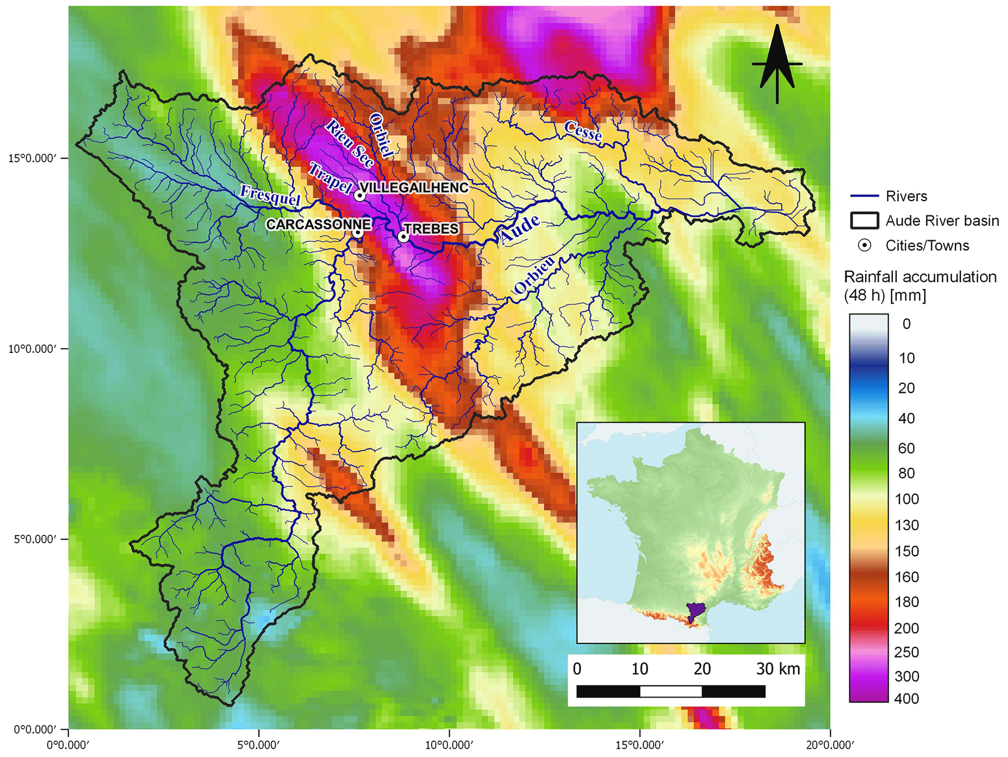
Figure 2 The Aude River basin, its river network and the rainfall accumulations observed from 14 October 2018 at 00:00 UTC to 15 October 2018 at 23:00 UTC according to the ANTILOPE J+1 quantitative precipitation estimates (see Sect. 3.2).

A major precipitation event occurred in this area from 14 to 16 October 2018, with particularly high rainfall accumulations during the night of 14 to 15 October. The maximum rainfall accumulations hit the intermediate part of the Aude River basin, just downstream the city of Carcassonne (Fig. 2). Up to 300 mm of point rainfall accumulation was observed (Caumont et al., 2021). The maximum accumulated rainfall amounts over short durations were also extreme: up to 60 mm in 1 h and 213 mm in 6 h recorded at Villegailhenc (Fig. 2), while the local 100-year rainfall accumulation is 200 mm in 6 h (Ayphassorho et al., 2019). By its intensity and spatial extent, the 2018 event nears the record storm and flood event that hit the Aude River basin in November 1999 (Gaume et al., 2004).

The October 2018 floods of the Aude River and its tributaries led to the activation of the highest (red) level of the French flood warning system “Vigicrues” (https://www.vigicrues.gouv.fr/, last access: 15 May 2023). They caused 14 deaths, about 100 injuries, and between EUR 130 and 180 million of insured damage (CCR, 2018). The floods were particularly severe on the tributaries affected by the most intense rains in the intermediate part of the Aude basin (Trapel, Rieu Sec, Orbiel, Lauquet) and also on the upstream parts of the Cesse and Orbieu tributaries (see Fig. 2). The peak discharge on the main Aude River at Trèbes reached the 100-year value (Ayphassorho et al., 2019) only 9 h after the onset of the rainfall event. In contrast, the peak discharges were high but not exceptional and caused limited inundation in the upstream and downstream parts of the Aude River basin. The high observed spatial and temporal rainfall and runoff variability makes this flash-flood event a challenging and interesting case study for the event-scale evaluation framework of short-range flood forecasts proposed in this study.

3.2 Observed hydrometeorological data

High-resolution quantitative precipitation estimates (QPEs) for the event were obtained from the Météo-France's ANTILOPE algorithm (Laurantin, 2008), which merges operational weather radar (30 radars operating in October 2018) and rain gauge observations, including not only real-time observations but all observations available 1 d after the event. These QPEs are called ANTILOPE J+1 hereafter. A comprehensive reanalysis of this product is available for the period from 1 January 2008 to 18 October 2018 at the hourly time step and 1 km × 1 km spatial resolution. This product was used in this study to calibrate and run the hydrological models.

Discharge series were retrieved from the French Hydro database (Leleu et al., 2014; Delaigue et al., 2020) for the 31 stream gauges located in the Aude River basin over the period 2008–2018. Additionally, peak discharges of the October 2018 flood event at ungauged locations were estimated during a post-flood field campaign (Lebouc et al., 2019) organized within the HYdrological cycle in the Mediterranean EXperiment (HyMeX, see https://www.hymex.org/, last access: 15 May 2023; Drobinski et al., 2014) research program.

Evapotranspiration values, necessary to run the continuous rainfall–runoff model, were estimated using the Oudin formula (Oudin et al., 2005), based on temperature data extracted from the SAFRAN meteorological reanalysis produced by Météo-France on an 8 km × 8 km square grid (Vidal et al., 2010).

3.3 AROME-based short-range rainfall ensemble forecast products

Rainfall forecasts are based on Météo-France's AROME-France NWP model (Seity et al., 2011; Brousseau et al., 2016). AROME-France is an operational limited-area model that provides deterministic weather forecasts up to 2 d ahead. Thanks to its high horizontal resolution, the model can explicitly resolve deep convection, which is well suited to forecast heavy precipitations. Three different AROME-based short-range rainfall ensemble forecast products were evaluated in this work.

• AROME-EPS is the operational ensemble version of AROME-France (Bouttier et al., 2012; Raynaud and Bouttier, 2016). AROME-EPS is derived from perturbations of model equations, initial conditions and large-scale coupling of the NWP model. In 2018, AROME-EPS was a 12-member ensemble forecast, updated every 6 h (four times per day: at 03:00, 09:00, 15:00 and 21:00 UTC) and providing forecasts up to 2 d ahead.

• pepi is an experimental product aiming to address the specific requirements for short-range flash-flood forecasting, i.e., high temporal and spatial resolutions, high refresh rate, and seamless forecasts. The pepi product is a combination of AROME-EPS and AROME-NWC (Auger et al., 2015). AROME-NWC is a configuration of AROME-France designed for now-casting purposes; it is updated every hour and provides forecasts up to 6 h ahead. In order to take into account sudden weather changes, AROME-NWC is used with time lagging (Osinski and Bouttier, 2018; Lu et al., 2007), which consisted here in using the last six successive runs of AROME-NWC instead of using only the most recent run. The resulting pepi product provides forecasts for a maximum lead time of 6 h. It combines 12 members from the last available AROME-EPS run and 1 to 6 members from AROME-NWC, depending on the considered lead time. The resulting number of members varies between 13 (for a 6 h lead time) and 18 (for a 1 h lead time).

• pertDpepi is a second experimental product, obtained by shifting the original pepi members 20 km in the four cardinal directions on top of the unperturbed pepi members to account for uncertainties in the forecast rainfall location. The number of members is 5 times the number of the “pepi” ensemble, i.e., varies from 65 to 90 members depending on the lead time. This product is based on the concepts proposed by Vincendon et al. (2011) but uses a simpler framework to derive the test product specifically designed for this study. The shift scale of 20 km represents a typical forecast location error scale: according to Vincendon et al. (2011), 80 % of location errors are less than 50 km. The value of 20 km has been empirically tuned to produce the largest possible ensemble spread on a set of similarly intense precipitation cases without noticeably degrading the ensemble predictive value as measured by user-oriented scores such as the area under the ROC curves.

These three rainfall forecast products have the same spatial (0.025^∘ × 0.025^∘) and temporal (1 h) resolutions and cover the same spatial window as AROME (metropolitan territory of France). For the comparison with rainfall observations, they were disaggregated on the corresponding 1 km × 1 km grid. In order to issue hydrological forecasts every hour, the last available runs of AROME-NWC and AROME-EPS (and the resulting pepi and pertDpepi ensembles) were systematically used according to the product updates. The AROME-NWC and AROME-EPS forecasts were supposed to be immediately available for each update (i.e., the computation delays were not considered).

3.4 Rainfall–runoff models

The ensemble rainfall forecasts were used as input for two rainfall–runoff models which differ in their resolution and structure. The GRSDi model is a semi-distributed continuous hydrological model adapted from the GRSD model (Le Moine et al., 2008; Lobligeois, 2014; de Lavenne et al., 2016) to better simulate autumn Mediterranean floods that typically occur after long dry summer periods (Peredo et al., 2022). The Cinecar model is an event-based distributed model, specifically developed to simulate flash floods of small ungauged headwater catchments, with limited calibration needs (Versini et al., 2010; Naulin et al., 2013; Le Bihan, 2016). Both models were calibrated against observations and presented good performance for the 2018 flood event, as presented below, where we provide more information about the models and their implementations.

The objective of this study is not to compare the rainfall–runoff models. Since the RS hydrographs (hydrographs simulated with ANTILOPE J+1 rainfall observations) are systematically used as reference for the evaluation of the flood forecasts, the evaluation results should not be directly dependent on the rainfall–runoff model but rather on the nature of the rainfall forecasts used as input. The interest of using two models here is mainly to strengthen the evaluation by involving two complementary models in terms of resolution and calibration approach: (a) because of its high spatial resolution, the Cinecar models help us to extend the evaluation of discharge threshold anticipation to small ungauged catchments, and (b) because it was not specifically calibrated on the 2018 event (calibration on the whole 2008–2018 period), the GRSDi model offers an evaluation of the total forecast errors at gauged outlets, including both the rainfall forecast errors and the rainfall–runoff modeling errors. This is achieved by the comparison of flood forecasts with both RS hydrographs and observed hydrographs. However, the proposed evaluation framework could also be applied by using one unique rainfall–runoff model.

3.4.1 GRSDi model

GRSDi is a reservoir-based hydrological model accounting for soil moisture that runs at an hourly time step with rainfall and evapotranspiration as input data. The model has seven parameters to be calibrated against observed discharges. For its implementation, the Aude River basin was divided into 123 modeling units (gray contours in Fig. 3a) of approximately 50 km². The model calibration and validation were performed for the same period (2008–2018), including the October 2018 flood event: 16 gauged outlets were selected for the calibration and 15 for the validation. The averaged KGE (Kling–Gupta efficiency; Gupta et al., 2009) values were 0.80 (0.71) for the 16 calibration outlets (15 validation outlets), which indicates good model performance except for one validation outlet, where a low KGE value of 0.1 was obtained (Fig. 3a). After visual inspection of the simulated discharges, this low performance was explained by an overestimation of the base flow, with however limited impact on the peak discharges during the high flows and flood events. The model and its performance evaluation is presented in details in Peredo et al. (2022).

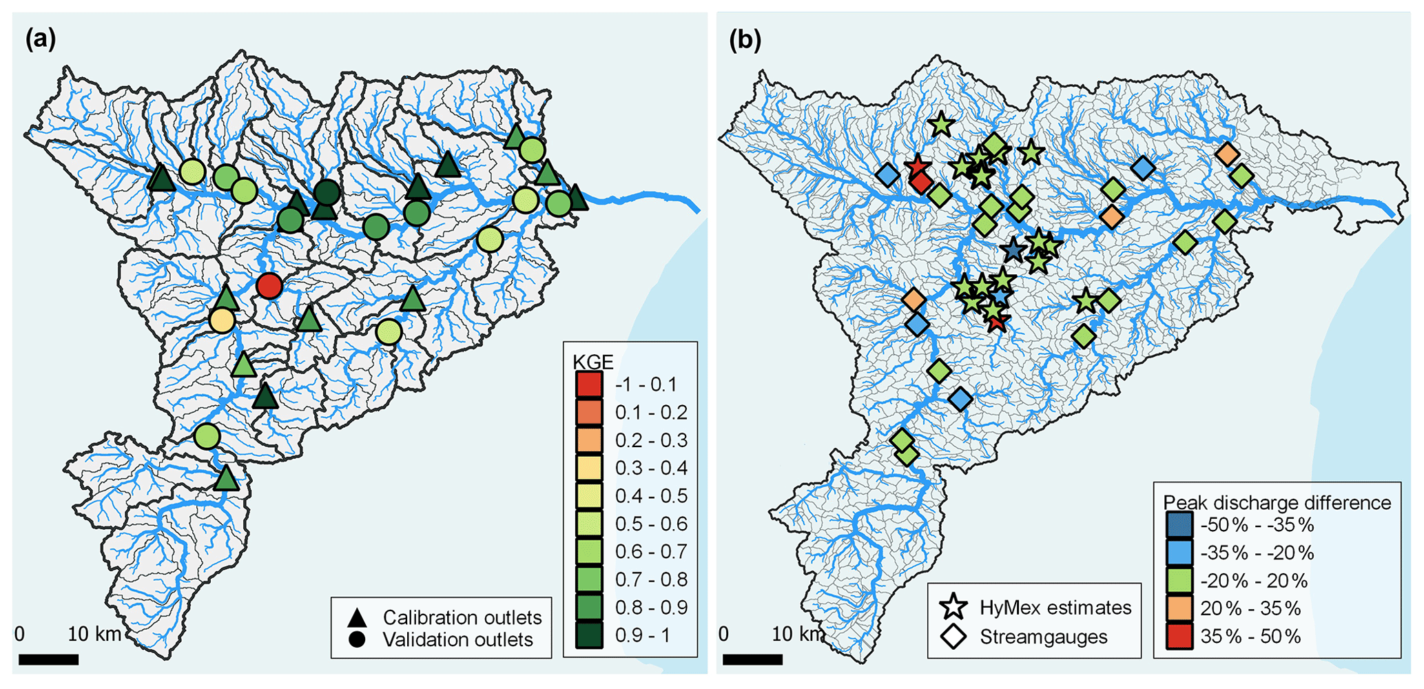
Figure 3 Calibration–validation results for the two rainfall–runoff models: (a) KGE values at calibration and validation outlets (stream gauges) for the GRSDi model and the period 1 October 2008 at 00:00 UTC to 15 October 2018 at 23:00 UTC and (b) peak discharge difference (in %) between Cinecar-simulated discharges and HyMeX (HYdrological cycle in the Mediterranean EXperiment) estimates (stars; Lebouc et al., 2019) or stream gauges (diamonds) when the model is calibrated over the Aude 2018 flood event.

3.4.2 Cinecar model

The Cinecar model combines a SCS-CN (Soil Conservation Service – curve number, CN) model for the generation of effective runoff on the hill slopes and a kinematic wave propagation model on the hill slopes and in the stream network. The model runs at a 15 min time step and was specifically developed to simulate fast runoff during flash floods, with a lesser focus on reproducing delayed recession limbs. The main parameter of the model requiring calibration is the CN (Naulin et al., 2013). For the implementation of the model, the Aude River basin was divided into 1174 sub-basins with an average area of 5 km² (gray contours in Fig. 3b). The shapes of the river reaches and hill slopes are simplified in the model, but their main geometric features (slopes, areas, length, width) are directly extracted from the digital terrain model (DTM). The CN values, first fixed on the basis of soil types and antecedent conditions, were further tuned to reach a better agreement between simulated and observed peak discharges for the Aude 2018 flood (Hocini et al., 2021). The resulting model was overall consistent with field observations, with errors in peak discharges generally in the ±20 % range (Fig. 3b).

4 Results

4.1 Overall performance of the rainfall ensemble forecast products

Figure 4 shows the temporal evolution of the hourly observed rainfall (ANTILOPE J+1) and the hourly forecast rainfall for the three ensemble products (AROME-EPS, pepi and pertDpepi) at 3 h of lead time from 14 October at 07:00 UTC to 15 October at 19:00 UTC. Figures corresponding to 1 and 6 h lead times are presented in Appendix A (Figs. A1 and A2). Rainfall intensities (millimeter per hour) are averaged over the entire Aude River basin area. Overall, the observed rainfalls are well captured by the forecast products. The ensemble forecast distributions are similar among the three products except for some time steps corresponding to the most intense rainfall period, where the added value of the AROME-NWC model used in the pepi and pertDpepi products can be noticed. As expected, the spread of the ensemble forecasts increases from AROME-EPS to pepi and pertDpepi, with some rare exceptions. This is in agreement with the increase in the number of ensemble members.

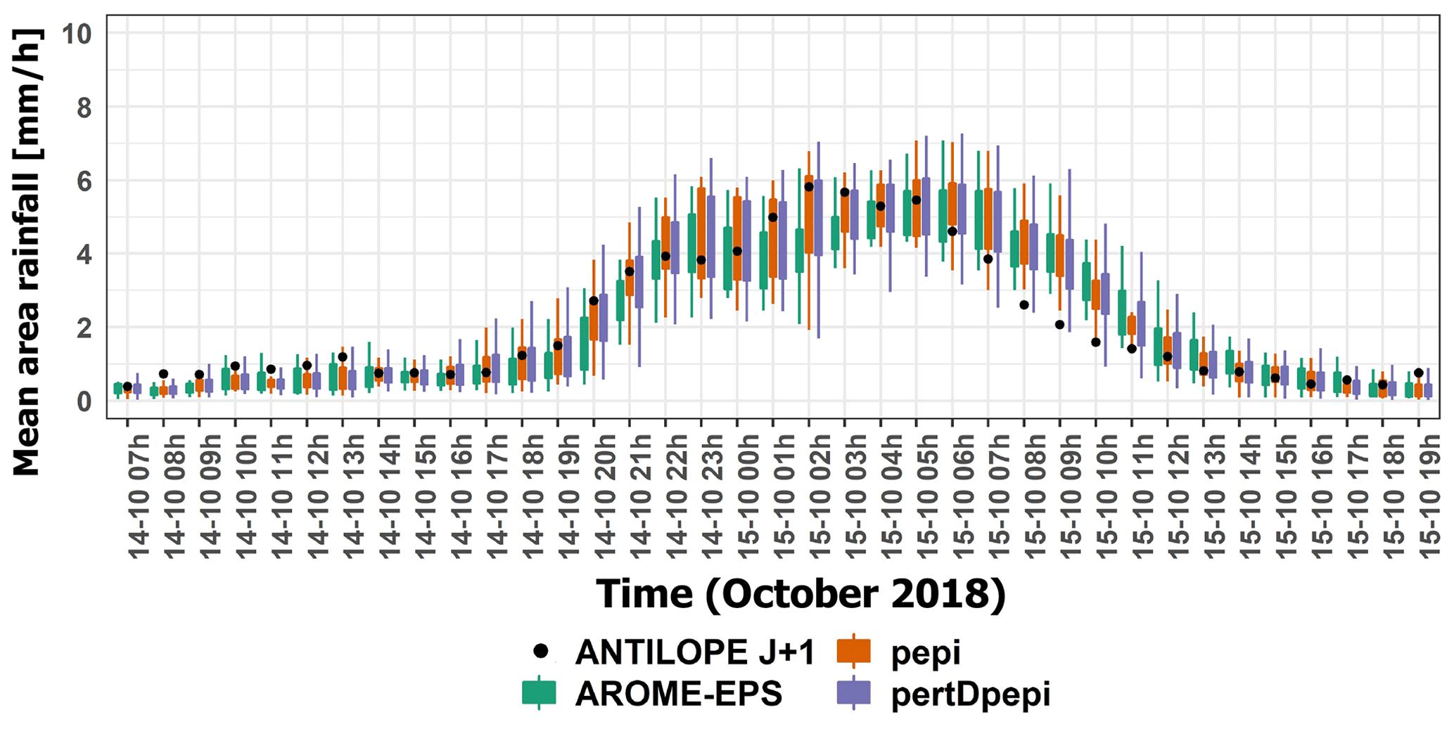
Figure 4 Temporal evolution of observed hourly rainfall rates (black dots), and 3 h lead time ensemble forecasts (boxplots) during the October 2018 flood event. Rainfall rates are averaged over the Aude River basin (6074 km²). The boxplots correspond to AROME-EPS (green), pepi (orange) and pertDpepi (purple). Whiskers reflect the min–max range and boxes the inter-percentile range (25th–75th) for the forecasts.

In general, the observed average rainfall rates are contained in the ensemble forecast ranges except at the end of the rainfall event on 15 October between 07:00 UTC and 11:00 UTC, where the ensemble forecasts overestimate the rainfall rates for the 3 and 6 h lead times. This is expected to have limited impact on the anticipation of floods, since it affects only the end of the rainfall event. The shape and magnitude of the average observed rainfall hyetograph is anticipated well by the 1 and 3 h lead time forecasts, while for the 6 h lead time forecasts a time-shift of 1 to 2 h is observed during the whole event. Even if not totally satisfactory, the time-shift remains significantly lower than the lead time of 6 h. This means that the rainfall forecasts are still helpful to anticipate the actually observed intense rainfall period, even if it is not perfectly positioned in time. This should result in an added value of the hydrometeorological ensemble forecasts to anticipate the flood rising limbs for this specific area and rainfall event.

As mentioned in Sect. 2, the objective of this first step is not only to evaluate the overall quality of the rainfall forecast products but also to define relevant space and time frames (HFA and HFT, respectively), which will help in illustrating the quality and usefulness of these products for flood forecasting. The selected space and time frames must include observed as well as forecast high intensities but not many areas or time steps with low intensities in both observation and forecasts. These areas are of little interest to flood forecasting, and they may mask the main features of the forecasts when carrying out an event-based forecast quality analysis. Based on the hyetographs presented in Fig. 4 and in Appendix A, the HFT was set from 14 October at 20:00 UTC to 15 October at 11:00 UTC. This corresponds to a 15 h period over which hourly observed and forecast average rainfall intensities on the Aude River basin were greater than 2 mm h⁻¹. The choice of this threshold is relatively subjective and just corresponds to a significant average rainfall intensity. Other threshold values could also have been selected. The choice of the HFA will be commented on below.

Figure 5 shows the spatial distribution of accumulated observed and forecast rainfall over the 15 h HFT time window. For the forecast products, the ensemble mean, the 75th percentile and the 95th percentile at 3 h lead time are plotted. The 1 and 6 h lead times are presented in Appendix A (Figs. A3 and A4). Note that the forecast panels do not correspond to rainfall accumulations for one unique run of forecasts but rather to a cumulated representation of the areas affected with high forecast rainfall intensities for the successive forecasts issued during the event. Figure 5 shows that the area affected by the high rainfall accumulations (over 280 mm within 15 h) is, in general, captured by the rainfall forecast products. The added value of the AROME-NWC model, generating locally more intense rainfall rates in the forecasts, can be seen by comparing the AROME-EPS and the pepi fields. The influence of the spatial shifts introduced in the pertDpepi product is also visible when comparing it with the pepi product. It is also interesting to note that the ensemble means are not able to capture the magnitude of the highest observed rainfall accumulations. Only the tail of the ensemble distributions at each pixel (75th and 95th percentiles) can approach the observed intensities. To produce hydrological forecasts based on a good estimate of the rainfall rates over the high rainfall accumulation period and area, it may be necessary to work based on a high ensemble percentile value (a least the 75th percentile in the present case study; Fig. 5e–g) rather than on the ensemble mean value. However, for these percentiles, the area of high intensity spreads and becomes larger than the area seen in the observed field of rainfall accumulations. This may be attributed to the location errors of some members in the successive runs of forecasts. This behavior is particularly marked in the pertDpepi product, which is probably a combined effect with the spatial shift in the perturbations introduced by this product. Finally, Fig. 5 also provides the required information to set the HFA. Even if not entirely hit by the observed heavy precipitation event, the Aude River basin is almost entirely covered with repeated high forecast rainfall intensities during the event, at least for the larger quantiles. This led to the choice of keeping the entire Aude River basin as the HFA. Considering this whole area will help in evaluating the risks of false alarms attributed to rainfall forecast location errors when forecasting floods. But as for the HFT, the choice of the exact limits of the HFA remains relatively subjective, and other extents of the HFA could also have been selected.

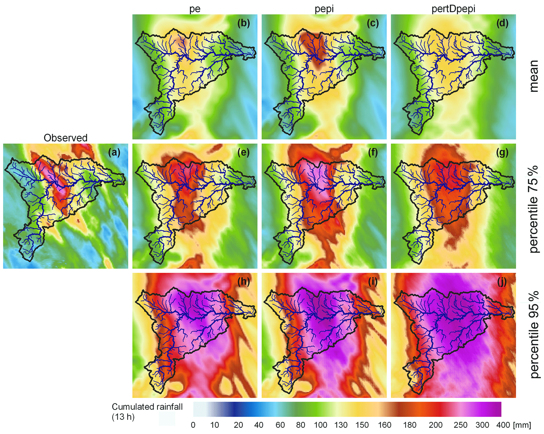
Figure 5 Comparison of observed and forecast (3 h lead time) rainfall amounts over 15 h (from 14 October at 20:00 UTC to 15 October at 11:00 UTC): (a) observed rainfall, (b, e, h) AROME-EPS ensemble mean and 75th and 95th percentiles, (c, f, i) pepi ensemble mean and 75th and 95th percentiles, and (d, g, j) pertDpepi ensemble mean and 75th and 95th percentiles.

The overall spread of the rainfall ensemble products can be further analyzed based on the rank diagrams presented in Fig. 6. The diagrams are plotted for a lead time of 3 h and pull together all the time steps within the HFT and the pixels of the HFA. Note also that they have been divided (i.e., stratified) into three subsamples according to the observed hourly rainfall intensities. The rank diagrams for 1 and 6 h lead times are available in Appendix A (Figs. A5 and A6). Overall, the U shape of the rank histograms indicates a lack of spread of the three ensemble products (under-dispersive ensembles), although still moderate, when it comes to capturing the observations within the ensemble spread at the right time and location. The histograms obtained for each subsample reveal a shift towards negative (positive) bias when the highest (lowest) observed rainfall intensities are considered. This bias appearing in the rank diagrams when datasets are stratified based on observed values, even for perfectly calibrated ensembles, is a well-documented phenomenon (Bellier et al., 2017). Observation-based stratification should therefore be considered with caution in forecast quality evaluations. It is nevertheless interesting to note the influence of stratification in the bias revealed by the rank diagrams. It can be a consequence of the limited spread of the ensemble rainfall forecasts. But it may also reflect the shifts and mismatches in time and space of the ensemble forecasts, already illustrated in Figs. 4 and 5.

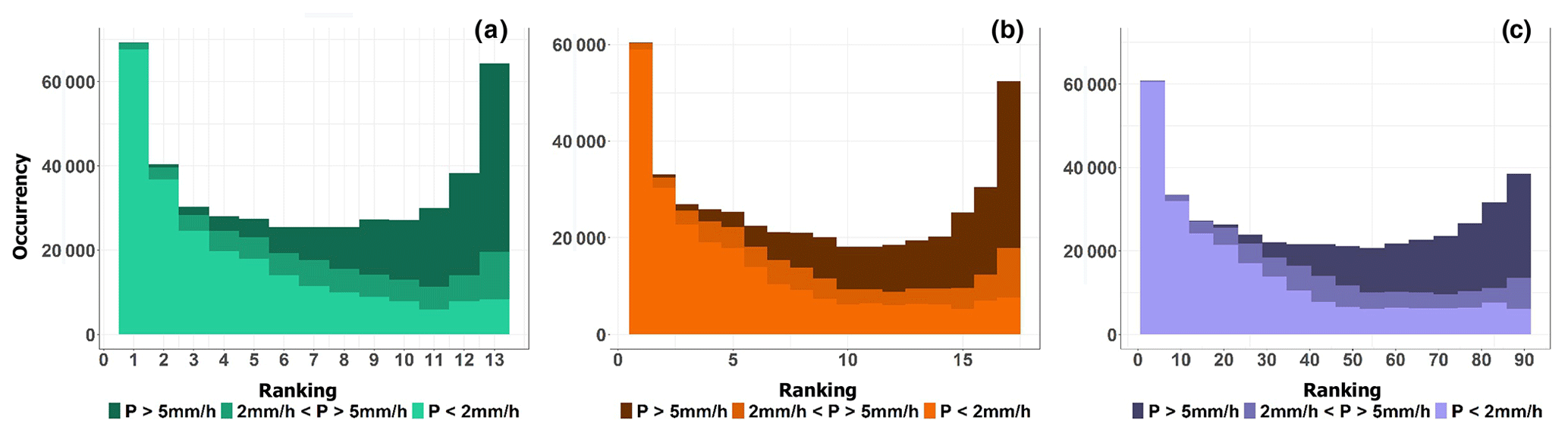
Figure 6 Rank diagrams of the three ensemble rainfall forecast products for rainfall rates under 2 mm h⁻¹, between 2 and 5 mm h⁻¹, and above 5 mm h⁻¹ and for a lead time of 3 h: (a) AROME-EPS, (b) pepi and (c) pertDpepi.

4.2 Hydrological anticipation capacity

As mentioned in Sect. 2, the hydrological forecasts are first evaluated on their ability to detect, with anticipation, the exceedance of predefined discharge thresholds. The objective is to provide a detailed and comprehensive view of the anticipation capacity for ungauged streams and main gauged rivers. The criteria and maps presented were computed based on the Cinecar hydrological model simulations and forecasts, and they include the entire sample of 1174 sub-basin outlets. The hydrological simulations based on observed ANTILOPE J+1 rainfall are considered the reference simulation (RS). The model is run from 14 October at 07:00 UTC and hourly rainfall accumulation are uniformly disaggregated to fit the 15 min time resolution of the model. The forecasts are issued every hour by using the ANTILOPE J+1 rainfall up to the time of forecast and one of the three rainfall forecast ensembles or a zero future rainfall scenario (RF0) for the next 6 h. The hydrological model is first run for each member of the rainfall forecast to generate a hydrological forecast ensemble. From this ensemble, at each hydrological outlet in the HFA, time series of forecast discharges are obtained for several probability thresholds.

The discharge thresholds correspond to the 10-year discharge return period, estimated by the SHYREG method (Aubert et al., 2014). This method provides flood quantiles estimates for all ungauged outlets with a drainage area exceeding 5 km². The choice of a 10-year return period was motivated by two main reasons: (i) this is a discharge level for which significant river overflows and damage are likely to be observed in many streams and (ii) according to the RS scenario, during the October 2018 flood event about half of the 1174 sub-basins in the HFA were hit by floods with peak discharge exceeding this threshold. It is also important to remember that six runs of forecasts and all lead times are combined at each outlet for the computation of the scores presented in this section (see Appendix B): i.e., one exceedance detected in advance, for at least one of the six forecast runs issued just before the exceedance, is considered to be a detection (hit). This means that one unique result (either a hit, a miss, a false alarm or a correct rejection) is obtained for each of the 1174 sub-basins and for each ensemble percentile.

Figure 7 illustrates the resulting ROC curves obtained for the hydrological ensemble forecasts based on the three rainfall products.

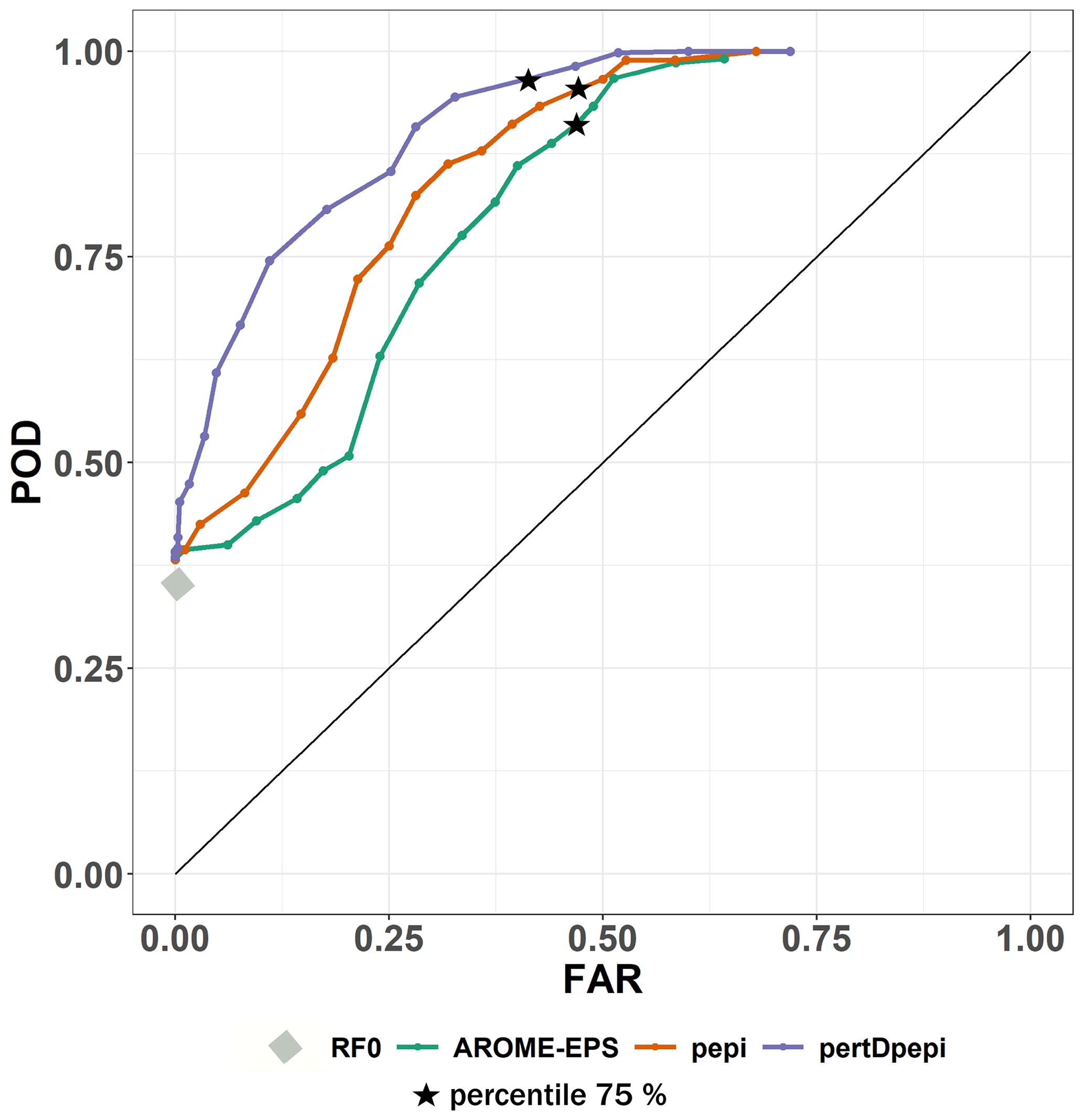
Figure 7 ROC curves (probability of detection as a function of false alarm rate) summarizing the anticipation of exceedances of the 10-year discharge threshold for the October 2018 flood event in the Aude River basin. The hydrological forecasts presented are based on AROME-EPS, pepi and pertDpepi rainfall ensemble products, as well as the Cinecar hydrological model. The black stars indicate the scores obtained for the 75th percentile of the hydrological ensemble forecasts. The points represent the scores obtained for the other percentiles from the 5th to 95th. The gray diamond shows the POD for the RF0 forecasts (zero-future rainfall forecast).

In the figure, the points related to the 75th percentiles of the ensembles are highlighted on each curve. The point obtained for forecasts using a zero rainfall scenario (RFO) is also presented. The added value of the pepi ensemble, compared to the AROME-EPS ensemble, was already observed in the forecast rainfall analysis (Sect. 4.1). It is also clearly visible here: for a selected ensemble percentile, both ensembles provide similar false alarm ratios, but the ensemble based on the pepi rainfall product has a higher probability of detection. For a spatial overview of the results, the maps of hits, misses, false alarms and correct rejections based on the 75th percentiles are presented in Fig. 8. In the central area of the Aude River basin, the missed detections for pepi ensemble are lower (26; Figs. 8c) when compared to the AROME-EPS ensemble (50; Fig. 8b). This is in line with the better capacity of the pepi ensemble forecast product to capture the observed high rainfall accumulations (Fig. 5). Overall, the use of the pertDpepi ensemble product leads to a reduction in the number of false alarms (255; Fig. 8d) when compared to the two other ensemble products (290 for AROME-EPS and 292 for pepi). In practice, the effects of the spatial perturbation introduced by the pertDpepi ensemble differ depending on the area and ensemble percentile considered: it leads to an increase in the area covered by high accumulated rainfalls when considering the highest percentile values of the rainfall ensembles, as clearly visible in Fig. 5 for the 95th percentile, but it may also have a smoothing effect of the high rainfall values when considering intermediate ensemble percentiles. This may be an explanation for the reduction in false alarms in some areas for the 75th percentile of the flood forecasts based on the pertDpepi product (Fig. 8).

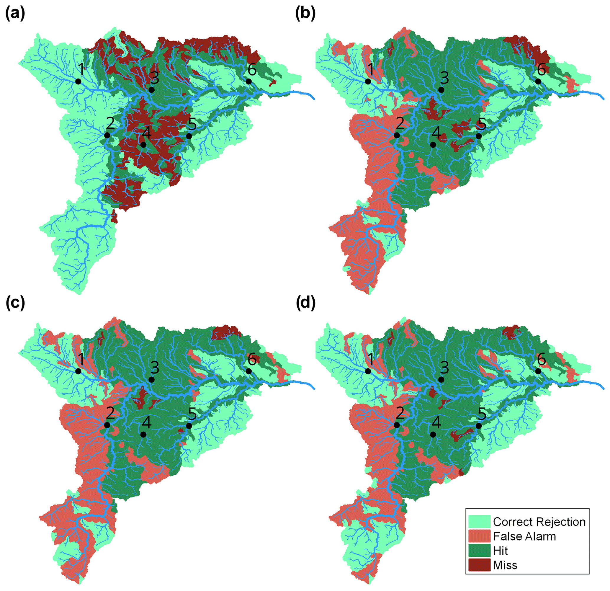
Figure 8 Maps illustrating the detailed anticipation results (hits, misses, false alarms, correct rejections) of the 10-year return period discharge threshold for the hydrological forecasts based on (a) RF0 scenario, (b) AROME-EPS ensemble (75th percentile), (c) pepi ensemble (75th percentile) and (d) pertDpepi ensemble (75th percentile). Hits are displayed for anticipation times exceeding 15 min. Black dots represent the outlets where a detailed analysis of the forecasts is proposed in Sect. 4.3.

The comparison of the ROC results of the ensemble hydrological forecasts with those of the RF0 scenario – i.e., future rainfall set equal to zero – helps us to further evaluate the added value of the rainfall forecast products. All ensemble forecasts lead to an increase in the number of hits (Fig. 8) and in the probability of detection (Fig. 7). However, this gain is obtained at the cost of an increase in the number of false alarms. When we look at the 75th percentile of the ensembles (black stars), close to 50 % of the sub-basins of the Aude River basin where the 10-year discharge return period is not exceeded are associated with a false alarm.

Figure 9 shows the distribution of anticipation times, within categories ranging from 15 min to 6 h, for sub-basins with hits in Fig. 8. Note that the anticipation time is defined here as the difference between the time of exceedance of the discharge threshold by the RS hydrograph and the time of the first run of forecasts that detects the threshold exceedance (see Appendix B). The figure also shows the number of sub-basins where either no anticipation (i.e., those with misses) or false alarms are observed and confirms the observations already made in Fig. 8: a lower number of false alarms for the ensemble forecasts based on the pertDpepi rainfall product when compared to AROME-EPS and pepi and a higher number of sub-basins associated with misses for forecasts of the RF0 reference scenario, as expected. But the results presented in Fig. 9 also confirm the added value of using the rainfall ensemble products to increase anticipation times of the exceedance of the 10-year discharge threshold: the anticipation times remain mostly between 15 min and 1 h for RF0 forecasts, whereas they exceed 2 h for more than a half of the hits with the three ensemble rainfall products. The use of the rainfall ensemble forecasts is key in the present case study to extend anticipation times beyond 2 h, even if this result remains specific to the considered event and cannot be extrapolated to future events.

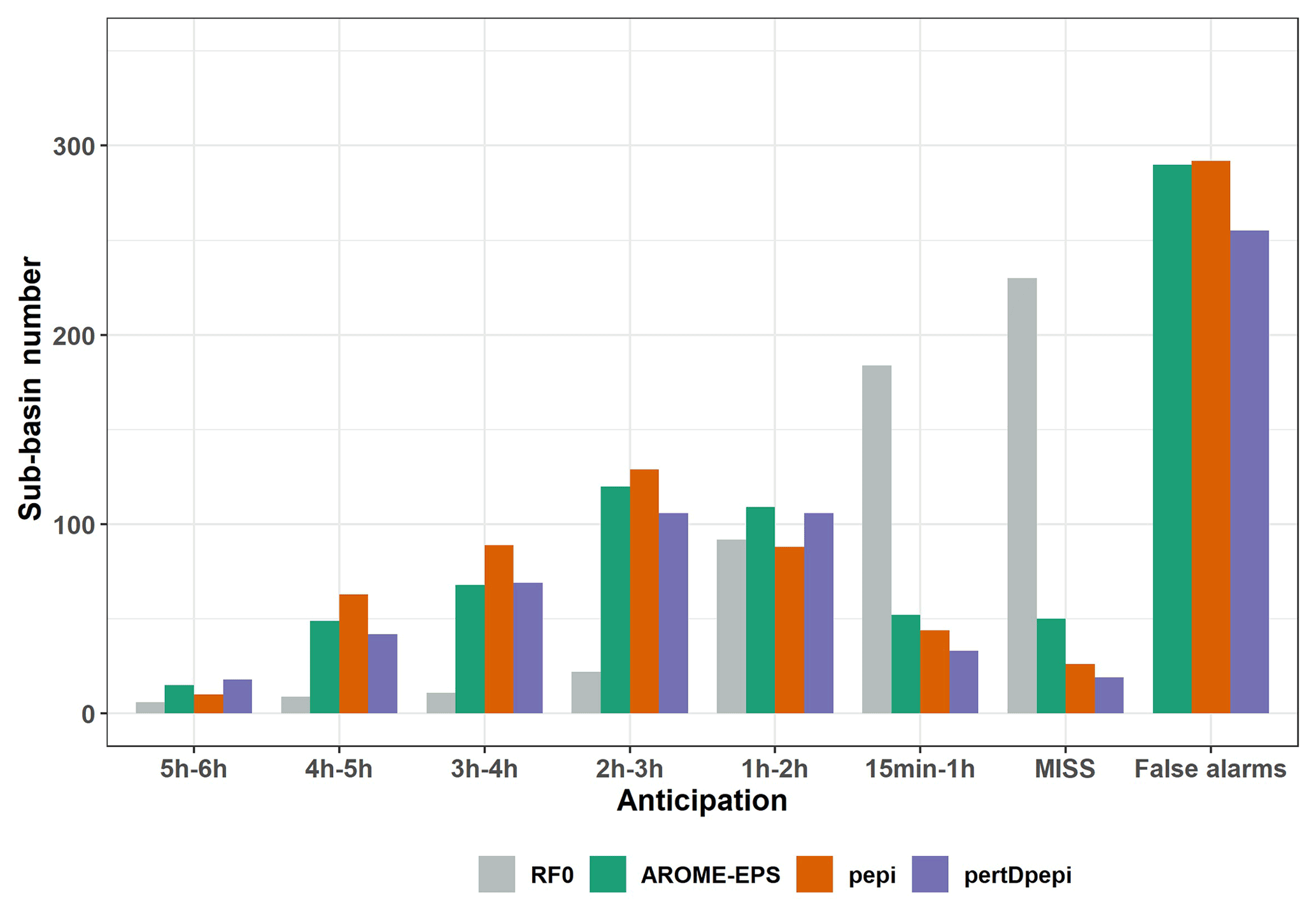
Figure 9 Comparison of 10-year threshold anticipation times for the hydrological forecasts based on the RF0 scenario and the three rainfall ensemble products. For the hydrological forecast ensembles, the 75th percentile is considered.

Figure 9 illustrates the necessary trade-off between gaining hits as well as larger anticipation times, and increasing false alarms as a consequence, when using ensemble hydrological forecasts to anticipate discharge threshold exceedances. Is it worth it compared to the RF0 forecasts (no future rainfall), where false alarms are avoided, but the number of misses is increased, and the anticipation times are lower, as in the case of the 2018 event? The answer to this question depends on the end users of the forecasts and their capabilities to respond to flood warnings. Further considerations on the cost and benefits associated with the hits and increased forecasting anticipation times, but also with the misses and false alarms, would be needed to fully address the question. For instance, in our case study, if we summarize the contingency tables used to draw Figs. 8 and 9 by using the percent correct (PC) score (Wilks, 2011) – i.e., the fraction of the N forecasts for which a forecast correctly anticipated the event (hit) or the no-event (correct rejection) – then the conclusion would be that the RF0 forecast outperforms the three ensemble hydrometeorological forecasts, at least when the decision is based on their 75th percentile. This is because the PC scores are 80 % for RF0, 71 % for AROME-EPS, 73 % for pepi and 77 % for pertDpepi. However, this score gives the same cost or benefit to misses, false alarms, hits and correct rejections. Additionally, it does not consider the added value of the increased anticipation of the threshold exceedances. This shows that an in-depth evaluation of hydrometeorological forecasts could strongly benefit from scores and metrics taking into account the end user's constraints and needs, as much as possible. This would help us to measure the actual cost–benefit balance of using hydrometeorological forecasts in real-time operations. Nevertheless, from the evaluation framework proposed here, we were able to identify that the hydrometeorological ensemble forecasts can offer better anticipation times than the RF0 forecasts, although this anticipation has a cost, i.e., an increase in the number of false alarms, which the user would need to be able to accept.

4.3 Detailed hydrological forecast evaluation at selected outlets

To complement the assessment results, a detailed analysis of the hydrometeorological forecasts is carried out at six selected gauged outlets, covering a variety of situations (see Fig. 8 for their location).

The results presented hereafter are based on the GRSDi model simulations and forecasts. The choice of this model is driven by the possibility of comparing the forecast hydrographs to both the simulated (RS scenario) and the observed hydrographs at gauging stations with a hydrological model which was not specifically calibrated to the 2018 flood. This allows us to compare errors related to the rainfall forecasts to those related to the modeling errors. Figures 10 to 15 present, for each of the six selected outlets, three panels of results. The first one on the left shows the spread–skill score of discharge forecasts for all lead times (1 to 6 h). The spread is the average of the standard deviation of ensemble forecasts. It is divided by the skill, which is the RMSE of the ensemble mean, to obtain the spread–skill score. A value of 1 means that spread and skill are equivalent. The other panels allow us to visually inspect the shape and spread of the forecast hydrographs (mean and quantiles of the ensemble forecasts) for an intermediate lead time of 3 h and to compare the forecasts to the simulated (RS) and observed discharges. Only pepi (middle panel) and pertDpepi (right panel) forecast hydrographs are presented (the AROME-EPS hydrographs are provided in Appendix C). It should be noted that the “forecast hydrographs” are represented for a fixed 3 h lead time and are not continuous discharges series in time as in the case of the observed and simulated hydrographs. They rather represent what could be predicted by the forecasts issued 3 h before each time step t of the flood event.

Outlets 1 and 2 (Figs. 10 and 11) correspond to weak hydrological reactions – i.e., the peak discharge of the reference simulation (RS) remains largely below the 10-year discharge threshold in both cases. At outlet 1, the previous step, i.e., the evaluation of discharge threshold anticipation capacity during the flood rising limb, showed a correct rejection, whereas at outlet 2 a false alarm was obtained with the three ensemble forecast products. Outlets 3 and 4 (Figs. 12 and 13) correspond to small-sized watersheds, located in the most intense observed rainfall area. For both outlets, the 10-year threshold exceedance could not be detected with significant anticipation with the RF0 forecast scenario (15 min of anticipation time for outlet 3, and 0 min – i.e., miss – for outlet 4), whereas anticipation times of 3 h 15 min were obtained with the three ensemble forecast products. Outlets 5 and 6 (Figs. 14 and 15) represent larger watersheds. At these outlets, the 10-year threshold exceedance could be anticipated with the RF0 forecast scenario (anticipation times of 45 and 60 min, respectively). However, these outlets also show an increase in the anticipation capacity with the ensemble rainfall forecasts: anticipation times ranging from 2 h 45 min to 4 h 45 min at outlet 5 depending on the rainfall forecast product and of 6 h at outlet 6 for the three products.

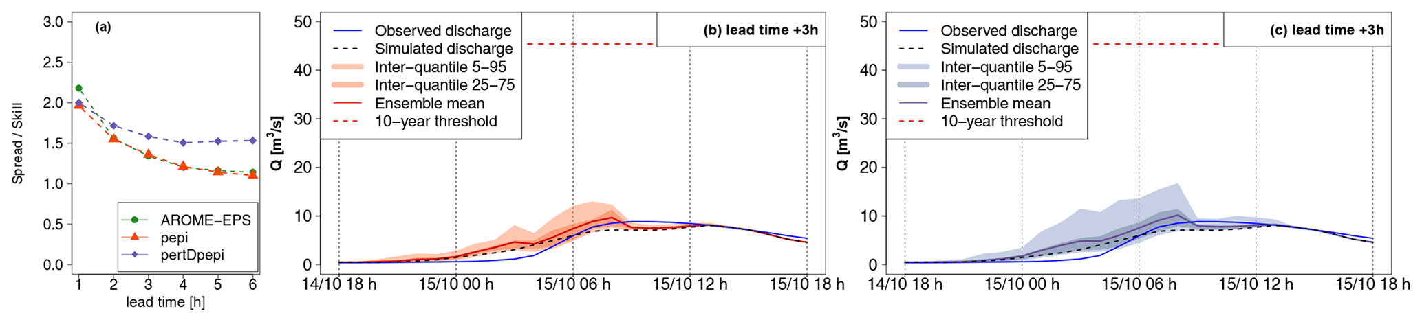
Figure 10 Detailed hydrological forecast evaluation at outlet 1 (216 km²): (a) spread–skill relationship, (b) hydrographs of 3 h lead time forecasts with pepi and (c) hydrographs of 3 h lead time forecasts with pertDpepi. In blue, the observed hydrograph at the gauging station.

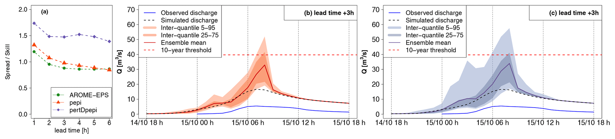
Figure 11 Detailed hydrological forecast evaluation at outlet 2 (197 km²): (a) spread–skill relationship, (b) hydrographs of 3 h lead time forecasts with pepi and (c) hydrographs of 3 h lead time forecasts with pertDpepi. In blue, the observed hydrograph at the gauging stations.

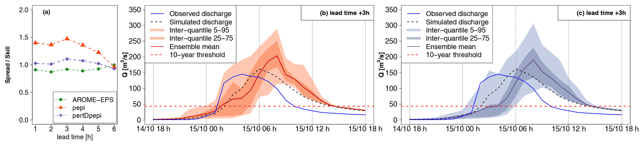
Figure 12 Detailed hydrological forecast evaluation at outlet 3 (85 km²): (a) spread–skill relationship, (b) hydrographs of 3 h lead time forecasts with pepi and (c) hydrographs of 3 h lead time forecasts with pertDpepi. In blue, the observed hydrograph at the gauging station.

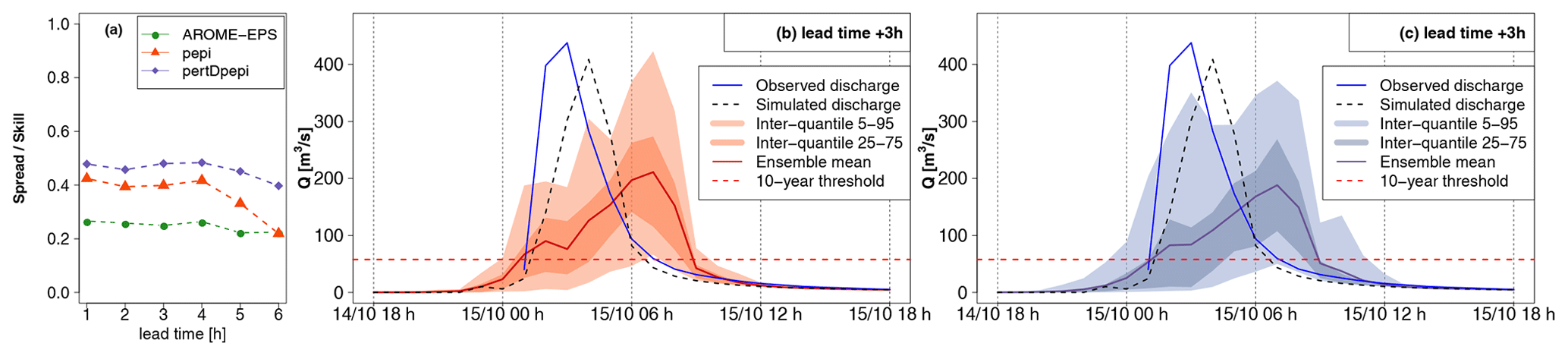
Figure 13 Detailed hydrological forecast evaluation at outlet 4 (173 km²): (a) spread–skill relationship, (b) hydrographs of 3 h lead time forecasts with pepi and (c) hydrographs of 3 h lead time forecasts with pertDpepi. In blue, the observed hydrograph at the gauging station.

For outlet 1, the simulated (RS) hydrograph is overall correctly retrieved by the forecasts (Fig. 10). For outlet 2, the forecast hydrographs show a larger dispersion and a significant overestimation, in particular for the upper percentiles (Fig. 11). This overestimation is present in the forecasts based on the three ensemble rainfall products. It explains the false alarm observed in Fig. 8, when the 75th percentile is considered. It is directly related to the overestimation of rainfall in areas surrounding the actually observed high rainfall accumulation area, as identified in Fig. 5. The spread–skill relationship scores (Figs. 10a and 11a) show that the hydrological ensemble forecasts tend to have a higher spread–skill score for the first lead times in all rainfall products. It becomes close to 1 after 2 to 4 h of lead time for the hydrological forecasts based on AROME-EPS and pepi rainfall products (i.e., the spread correlates well with the errors). For the forecasts based on pertDpepi, the score tends to stabilize around 1.5 (i.e., there is 50 % more spread than ensemble mean skill in these forecasts), highlighting a shortcoming of potentially overly – or unnecessarily – widespread rainfall in this ensemble product. It might be caused by an excessive spatial shift with respect to the geographical size of the investigated catchment. The larger dispersion of the pertDpepi forecast ensemble is confirmed by the hydrographs and is in particular visible for the 5th–95th percentile inter-quantile range, while the range defined by the 25th and 75th percentiles show limited difference with the respective inter-quantile range in the pepi ensemble product. This confirms the tendency of the pertDpepi rainfall product to modify differently the extreme percentiles and the intermediate ones when compared to pepi. In practice, the over-dispersion observed for extreme percentiles could have limited the performance of the pertDpepi ensemble if these extreme percentiles had been used by a user. This was also visible in Fig. 7: a large increase in false alarm rates with the pertDpepi ensemble product in the upper part of the ROC curve.

Lastly, the comparison of observed and simulated hydrographs shows a different performance of the hydrological model between outlets 1 and 2. The modeling errors are limited in the case of outlet 1, whereas the observed discharges are overestimated by the model in the case of outlet 2. In this second case, the comparison between observed, simulated and forecast hydrographs shows that a large part of the total forecast error can be attributed to modeling errors.

In the cases of outlets 3 and 4 (small size watersheds in the most intense observed rainfall area; Figs. 12 and 13), the RS hydrograph largely exceeds the 10-year discharge threshold at the very beginning of the flood rising limb. The 3 h forecasts also exceed the thresholds and anticipate well the initial increase in the river discharges. This results in the hits presented in Fig. 8 and in the good anticipation times, exceeding 3 h for both outlets. A forecast user could be satisfied with such information (anticipation of threshold exceedance) to start a flood response.

For both outlets, the forecast hydrographs show a delay in the flood rising limb and flood peak, comparatively to the simulated hydrographs. This means that shortcomings are present in the rainfall forecast products in terms of the dynamics of the time evolution of the rainfall event. These shortcomings could not be directly captured in the previous evaluation scores but might be an important feature for forecast users. The flood rising limb is overall better represented in the case of outlet 3. At outlet 4, the 3 h simulated hydrograph presents a large delay comparatively to the simulated hydrographs (3 h between observed and 75th percentile 3 h forecast peak discharges). This delay comes with a significant underestimation of the flood peak magnitude by the ensemble mean and 75th percentile, although the 95th percentile is closer to the simulated discharge peaks. This goes along with the general tendency of the rainfall ensemble means to underestimate the higher rainfall accumulations (Figs. 5 and 6).

For both outlets, the spread–skill relationship scores reflect the influence of the temporal shifts between the simulated and forecast hydrographs. At outlet 3, where forecasts better resemble the simulated hydrographs, the spread–skill relationship is close to 1 for the ensembles based on AROME-EPS and pertDpepi, which can be interpreted as a sufficient variance of the forecast spread to cover the errors. The ensemble based on pepi, on the contrary, has 1.5 times more spread than skill at 3 h of lead time. At outlet 4, the disparity between forecast and simulated hydrographs is too high, and, the large forecast spread, as seen in the hydrographs, is not enough to cover the timing errors. At both outlets, and comparatively to outlets 1 and 2, we also note that the spread–skill relationship score almost does not change with forecast lead time except for pepi-based forecast at the longer lead times.

The comparison of observed hydrographs with simulated and forecast hydrographs also provides interesting information about the relative importance of modeling and forecasting errors. At outlet 3, the observed and simulated hydrographs have a different shape, whereas the simulated and forecast hydrographs appear similar despite a time delay. At outlet 4, observed and simulated discharges resemble each other (despite a time delay), but both are very different from the forecast hydrograph. This indicates that modeling errors are a major source of uncertainty at outlet 3 (if we consider that observations represent well the true flow values), comparatively to rainfall forecast errors, while the opposite is seen at outlet 4.

Finally, Figs. 14 and 15 present the forecast results obtained for outlets 5 and 6, corresponding to outlets at which significant anticipation is possible even without rainfall forecasts (RF0 scenario; see Fig. 8a). It can be seen that the hydrological reactions at these outlets are important, as the 10-year discharge threshold is exceeded by the RS hydrograph in the intermediate phase of the flood rising limb, although not as much as for outlets 3 and 4, where the discharges largely exceeded this threshold. This is explained by the location of these catchments, at the limits of the most intense observed rainfall area. Overall, the forecast hydrographs are less dispersed than in the preceding cases, and the differences between the three rainfall forecast products is less evident, with only a slightly larger spread for the forecasts based on the pertDpepi ensembles. This lower difference between products can be a direct result of the larger influence of flood propagation in the hydrological forecast, limiting the influence of rainfall forecast uncertainties in comparison with the former cases. However, some shortcomings of the rainfall forecasts are still visible in both cases. At outlet 5, the flood rising limb of the simulated hydrograph is well captured by the 25 %–75 % inter-quantile range of the 3 h ahead forecasts, but the forecasts display a delay of about 2 h in terms of timing of the peak discharge. This time-shift of forecasts may explain the misses that appear in the upstream parts of the catchment (Fig. 8). At outlet 6, the forecasts tend to slightly overestimate the peak of the simulated hydrograph, although the 5 % quantiles remain close to the simulated peak.

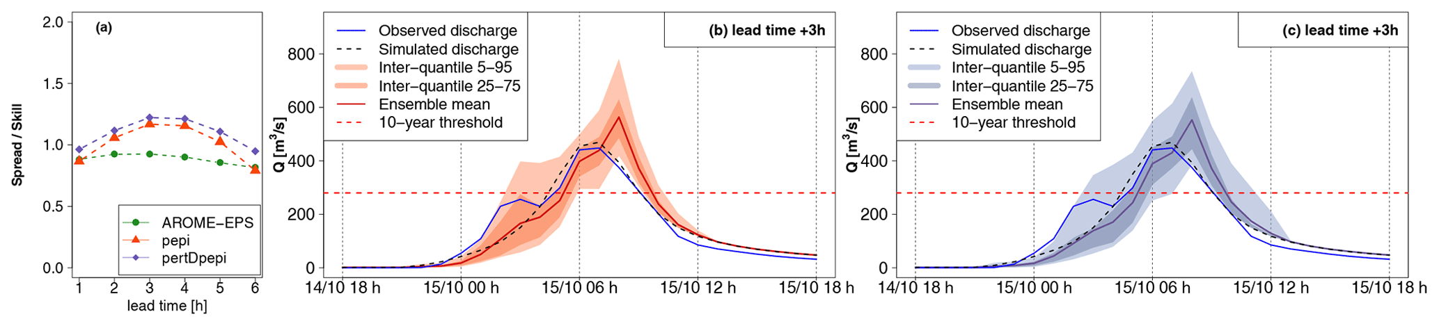
Figure 14 Detailed hydrological forecast evaluation at outlet 5 (263 km²): (a) spread–skill relationship, (b) hydrographs of 3 h lead time forecasts with pepi and (c) hydrographs of 3 h lead time forecasts with pertDpepi. In blue, the observed hydrograph at the gauging station.

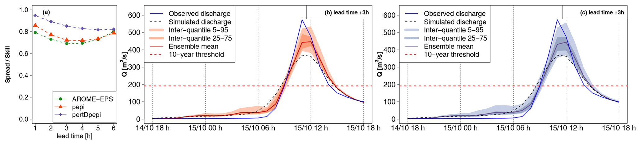
Figure 15 Detailed hydrological forecast evaluation at outlet 6 (257 km²): (a) spread–skill relationship, (b) hydrographs of 3 h lead time forecasts with pepi and (c) hydrographs of 3 h lead time forecasts with pertDpepi. In blue, the observed hydrograph at the gauging station.

The influence of modeling errors also clearly appears here. At outlet 5, simulated and observed hydrographs are close to each other during the main peak, but the first peak of the observed hydrograph is not represented in the simulation. At outlet 6, the simulated discharges follow the same pattern as the observed discharges, but the magnitude of the peak discharge is underestimated by the model. In both cases, the modeling errors are partially compensated for in the forecasts, under the condition that a user looks at the higher quantiles of the ensemble forecasts, as the 5 %–95 % inter-quantile range of the 3 h ahead forecasts gets closer to the observed peak discharges. Overall, these two outlets mainly illustrate how the evaluation of hydrological forecasts can be influenced also by the ability of the rainfall–runoff model to correctly represent the flood dynamics, when the evaluation is achieved based on actual flow observations.

5 Discussion

5.1 Added value and limitations of the implemented evaluation framework

After an initial analysis of the performance of the three rainfall forecast products, the evaluation procedure proposed in this paper focused on the capacity of the hydrological forecasts to anticipate the exceedance of selected discharge thresholds. Several authors have suggested using thresholds and contingency tables to perform a robust regional evaluation of hydrological ensemble forecasts (Silvestro and Rebora, 2012; Anderson et al., 2019; Sayama et al., 2020). In this study, a step further is proposed towards (i) focusing only on the rising limb phase of the flood hydrograph – i.e., the most critical phase in terms of anticipation needs for preparedness and emergency response, as already suggested by Anderson et al. (2019) – and (ii) splitting the analysis into a geographical point of view (discharge threshold anticipation maps) and a temporal point of view (histogram of anticipation times). The illustrative example of the October 2018 flood in the Aude River basin in France showed that this approach provides synthetic and meaningful information about the possible gains in anticipation compared with the RF0 reference forecast where future rainfalls are considered null. It also informs about the relative performance of the evaluated rainfall forecast ensemble products, even if the products appeared relatively similar at first sight in the example shown here. This analysis can be easily adapted to other flash-flood events with different characteristics or even to other types of floods. For instance, different discharge thresholds can be set to better distinguish the areas where the main flood reactions were observed, a larger threshold can be applied to the anticipation time to decide for a hit (a minimum threshold of 15 min of anticipation time was used in this study), and different ensemble percentiles can be selected to better illustrate the role that the probability threshold plays when evaluating different forecast products.

The threshold anticipation maps are also helpful for the selection of outlets where hydrographs should be analyzed in more details in the last phase of the evaluation. They avoid focusing only on outlets where large anticipation is possible without rainfall forecasts (RF0 scenario). The differences between the hydrological forecasts based on rainfall ensemble products may be more difficult to identify at these outlets because of the large influence of flood propagation in the hydrological forecasts. The threshold anticipation maps also allow selecting outlets corresponding to a variety of situations (i.e., hit, miss, false alarm, or correct rejection), which may help in bringing up details about the complex features of the hydrological ensemble forecasts.

If the proposed approach has several advantages, it also relies on several methodological choices which could be adapted or improved. It can be noted that only the runs of forecasts covering the most critical phase of the event (i.e., the time of the threshold exceedance or the maximum of the RS hydrograph) were considered to build the contingency tables. The results obtained could differ if other runs of forecasts and/or other phases of the event were considered. Particularly, in the case of events with multiple flood peaks, the fact that the method focuses only on the first threshold exceedance can be seen as a limitation. In such a situation, each rising phase of the flood event could be examined separately, even if in some cases the different phases of the floods may be difficult to separate. An alternative could be to analyze the anticipation of threshold exceedances for each run of forecasts during the event, independently of the times the thresholds are exceeded for the RS hydrographs. Providing an evaluation for multiple flood events, or for multiple thresholds for the same flood, may also be interesting complements to the results presented here. This may nevertheless cause some difficulties in setting the HFT and HFA, which are event specific. The HFA may also require being adapted to the considered threshold. To avoid changing the limits of the HFA, an option could be to use a score that does not account for correct rejections and therefore would be less sensitive to the extent of the HFA, such as the critical success index. In addition, the procedure used for the computation of the contingency tables and the anticipation times can be considered optimistic, at least in some situations. At first, as explained by Richardson et al. (2020), having a sequence of several consistent forecasts is often a desired quality in forecasting systems. Specific tests of the consistency of forecasts have been proposed (Ehret and Zehe, 2011; Pappenberger et al., 2011). In this study, only the first run of forecast exceeding the discharge threshold value was considered for defining a hit (or a false alarm), and the anticipation time was computed without considering the consistency of several successive forecasts. This can be seen to be pertinent when dealing with flash floods, when it is often not possible to wait for forecast consistency in real time to activate flood response actions. However, it could also be interesting to use the same method and to consider the number of runs correctly anticipating the threshold exceedances (or non-exceedances) to fill the contingency table. Moreover, since two of the three rainfall products used in this study are still experimental (pepi and pertDpepi) and are not yet included in the real-time production workflow of Météo-France, it was not possible to integrate the actual delivery times of the forecasts in this study. To obtain a more realistic view of the actual anticipation capacity, the delivery times of the different rainfall forecast products need to be integrated in the computation of the contingency tables and anticipation times, as proposed by Lovat et al. (2022). This means that the hydrological ensemble forecasts should be considered only from the delivery time of the rainfall forecast products used as input instead of from the beginning of the sequence of time covered by the rainfall forecasts. This integration would probably lead to a reduction in the number of hits and in the anticipation times obtained with the hydrological ensemble forecasts in this study, whereas it would not affect the results obtained for the RF0 forecast, where no future rainfall scenario is used.

Lastly, it should also be noted that the last step of the evaluation analysis proposed in this study, which is based on the whole hydrographs and spread and skill scores, remains essential to provide a detailed view of the strengths and limits of the different ensemble products evaluated. Particularly, the shortcomings of an ensemble with a dispersion that is too large (which is the case of the pertDpepi product) and the impact of temporal shifts on the quality of the forecasts would have been more difficult to identify without this last step of the analysis. The analysis of hydrographs also provides detailed explanations for the hits, misses, false alarms or correct rejections observed on the discharge threshold anticipation maps.

5.2 Performance of the three ensemble forecast products

The contribution of the rainfall forecast ensemble products to the anticipation of discharge thresholds, with respect to the scenario where no future rainfall forecast is available (RF0 scenario), was clearly illustrated here. This contribution lies mainly in the high reduction in the number of misses on the threshold anticipation maps (Fig. 8) and in a significant gain in the anticipation times for almost all sub-basins (Fig. 9). It also depends on the ensemble probability (or percentile) that is considered to define a forecast event (in our case, the 75th percentile). The use of ensemble forecasts was essential to obtain anticipation times greater than 1 h when a hit was observed, even if this positive effect was counterbalanced by the occurrence of a high number of false alarms in other areas of the catchment. This implies that, in order to conclude about the added value of ensemble forecasts, it is necessary to consider the balance between the actual gains and costs for a given user of the forecasts (Verkade and Werner, 2011). Hydrometeorological forecasting is no exception to the well-known decision principle: the larger the uncertainties (i.e., the lower the sharpness) affecting the predictions of the variable(s) on which the decision is based, the larger the safety margin will be to guard against the risk of unwanted consequences. Particularly in the case of flash floods, the user is often interested in reducing misses and increasing hits and anticipation times. This means that users need to consider how much of a false alarm rate they can handle and how much risk they can take (i.e., what percentile of the ensemble distribution they should consider). These are, however, difficult questions to answer. More flood event evaluations are needed to enhance our understanding of these trade-offs.

In the present case study, the pepi rainfall ensemble product was built from the AROME-EPS product by adding one to six additional members (depending on the lead time). This strategy had globally a positive influence on the quality of the ensemble forecasts, with a significant decrease in the number of misses for an equivalent number of false alarms (Fig. 9). This can be directly related to the increased reliability of the pepi forecasts compared to the AROME-EPS forecasts and therefore the better capture of the high rainfall accumulation periods (Fig. 4) and extension (Fig. 5) when considering the 75th percentile. Finally, in the case of this event, the pepi product provides an added value for the characterization of the main intense rain cell without a significant degradation of the ensemble performance in the surrounding areas, where the rainfall accumulations were less intense. However, this overall improvement does not result in a significant increase in the anticipation times obtained with the pepi product compared to the AROME-EPS product (Fig. 9).

Adding spatial perturbations in the four cardinal directions to the members of the pepi ensemble led to an increase in the number of members in the pertDpepi ensemble product, which varies from 65 to 90 members depending on the lead time. Overall, this resulted in a larger dispersion of the ensemble, particularly visible on the extreme percentiles (5th–95th), and led to positive as well as negative effects, both visible in the evaluation results. The high rainfall accumulation period is still well captured (Fig. 4), but the maximum rainfall area is not as well localized, comparatively to the observations, as for the pepi ensemble (Fig. 5). Regarding the discharge threshold anticipation maps (Fig. 8c and d), the reduction in the number of false alarms with pertDpepi is mainly due to the choice of the 75th percentile, which is not modified in the same way as higher percentiles when compared to the pepi ensemble. This is confirmed by the hydrograph analyses (Figs. 10 to 15), which overall confirm the over-dispersion of pertDpepi for higher percentiles of the ensemble distribution.

Moreover, the anticipation times are slightly reduced with pertDpepi when compared to the two other ensemble products (Fig. 9): 221 (over 1174) sub-basins show an anticipation time of more than 2 h against 245 for AROME-EPS and 259 for pepi. Again, the detailed hydrograph analyses (Figs. 10 to 15) confirm that pertDpepi does not efficiently compensate the time-shifts in the representation of hydrographs. The addition of spatial perturbations leads to a significant increase in the number of members, which significantly increases the computing times with the pertDpepi rainfall ensemble product (up to 72 additional members compared to pepi), but there is no clear benefit in adding these members in the case evaluated here.

6 Conclusions

In this paper, we proposed and tested a methodological framework for the evaluation of short-range flash-flood hydrometeorological ensemble forecasts at the event scale. Focusing on the evaluation of a single flood event is necessary because of (i) the relatively low frequency of flash-flood occurrences and (ii) the limited length of available re-forecast periods for newly developed ensemble rainfall forecast products based on convection-permitting NWP models. In order to enhance the value of a single-event evaluation, the point of view of an end user of the forecasts is adopted in the proposed methodological approach. This approach combines different steps. Firstly, it comprises a preliminary analysis of rainfall observations and forecasts, which provides a first overview of the quality of the ensemble rainfall products and information needed to select the most relevant ensemble percentile and spatial and temporal scales for the analysis. Secondly, a hydrological forecast analysis evaluates the detection of discharge threshold exceedances and the corresponding anticipation times. It considers the flood rising limb of the hydrographs and illustrates the gains in anticipation comparatively to a reference scenario where zero rainfall is forecast for the future. Thirdly, a detailed analysis of forecast hydrographs and spread–skill scores at outlets selected based on the former step is carried out. It aims to better illustrate the skills and the limits of the evaluated hydrological ensembles. This methodology was tested and illustrated with the major flash-flood event that hit the Aude River basin in southeastern France in October 2018. Three ensemble rainfall forecast products recently developed by Météo-France were compared, i.e., the AROME-EPS ensemble (12 members), the pepi ensemble combining AROME-EPS and AROME-NWC members (13 to 18 members), and the pertDpepi ensemble adding spatial perturbations to the pepi ensemble (65 to 90 members).

The study illustrated the multifaceted and complex issue of evaluating single flood events. It confirmed the interest of the proposed evaluation procedure to help forecast users to efficiently define beforehand the space and time windows to be used for the forecast performance evaluation. This was achieved by comparing the observed and forecast rainfall hyetographs and accumulations over the entire catchment area (step 1). The analysis of discharge threshold exceedance detection (step 2) contributed to illustrate the geographical features of the flood event and the anticipation capacities offered by each of the rainfall ensemble products. The comparison with a zero rainfall future scenario confirmed the gains in anticipation offered by the ensembles. From the threshold anticipation maps, it was also possible to select outlets that correspond to a variety of situations of interest to a forecast user (hits, misses, false alarms, correct rejections). These outlets could then be investigated in more detail based on observed, simulated (with observed rainfall as input to the hydrological model) and forecast hydrographs (step 3). This last phase illustrated further strengths and limitations of the different rainfall forecast products, including the shifts in timing that affect forecast skill and the main sources of forecast errors (rainfall forecasts or hydrological model).

The evaluation finally led to balanced conclusions about the three products of rainfall ensemble forecasts. These products clearly enhance the anticipation times when compared to a zero-rainfall future scenario but tend to overestimate the spatial extent of the area of the highest rainfall accumulations. This results in a higher risk of overestimating flood threshold exceedances in the surroundings of this area (i.e., an increase in false alarms). The actual added value of the evaluated forecasts for an end user therefore depends on the relative benefits of the increased anticipation and costs of the false alarms. However, the results also showed a hierarchy between the three evaluated products, and a clear added value of the pepi ensemble product could be identified. According to the significant time-shifts of forecast hydrographs in several sub-basins, which seem to significantly limit the anticipation times, the introduction of temporal perturbations could probably be an interesting alternative to be tested

Finally, even if evaluating ensemble hydrological forecasts based on a single flood event remains a very challenging issue due to the limited statistical representation of the available data, single-event evaluations are needed and important to advance operational flood forecasting systems. The evaluation framework proposed in this study could be helpful in drawing rapid and meaningful analyses of newly developed rainfall ensemble forecast approaches.

Appendix A: Comparison of observed rainfall and ensemble forecasts for 1 and 6 h lead times (hourly rainfall rates, maps of rainfall amounts, and rank diagrams

A1 Temporal evolution of observed hourly rainfall rates and ensemble forecasts for 1 and 6 h lead times

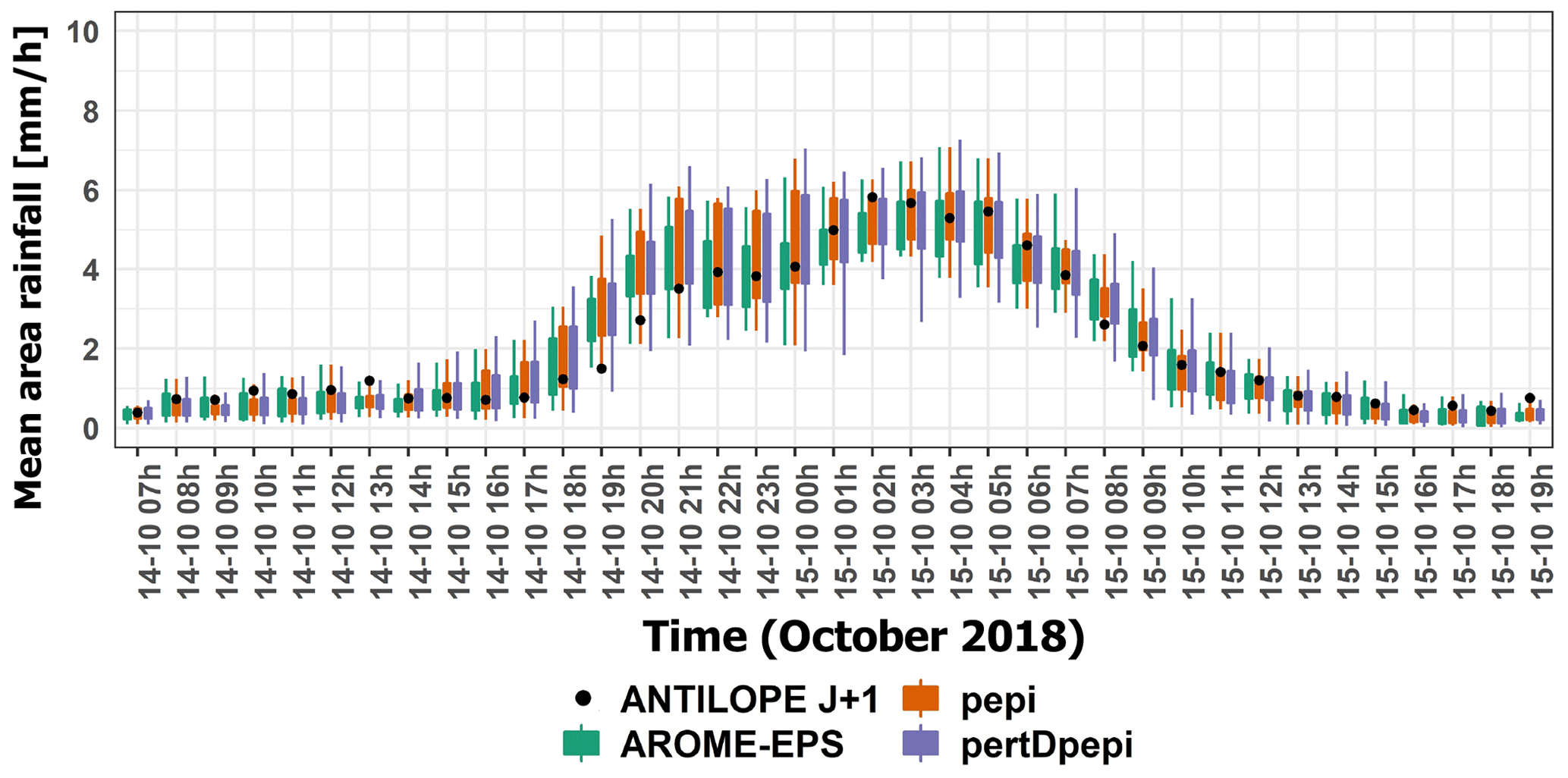
Figure A1 Temporal evolution of observed hourly rainfall rates (black dots) and 1 h lead time ensemble forecasts (boxplots) during the October 2018 flood event. Rainfall rates are averaged over the Aude River basin (6074 km²). The boxplots correspond to AROME-EPS (green), pepi (orange) and pertDpepi (purple). Whiskers reflect the min–max range and boxes the inter-percentile (25th–75th) for the forecasts.

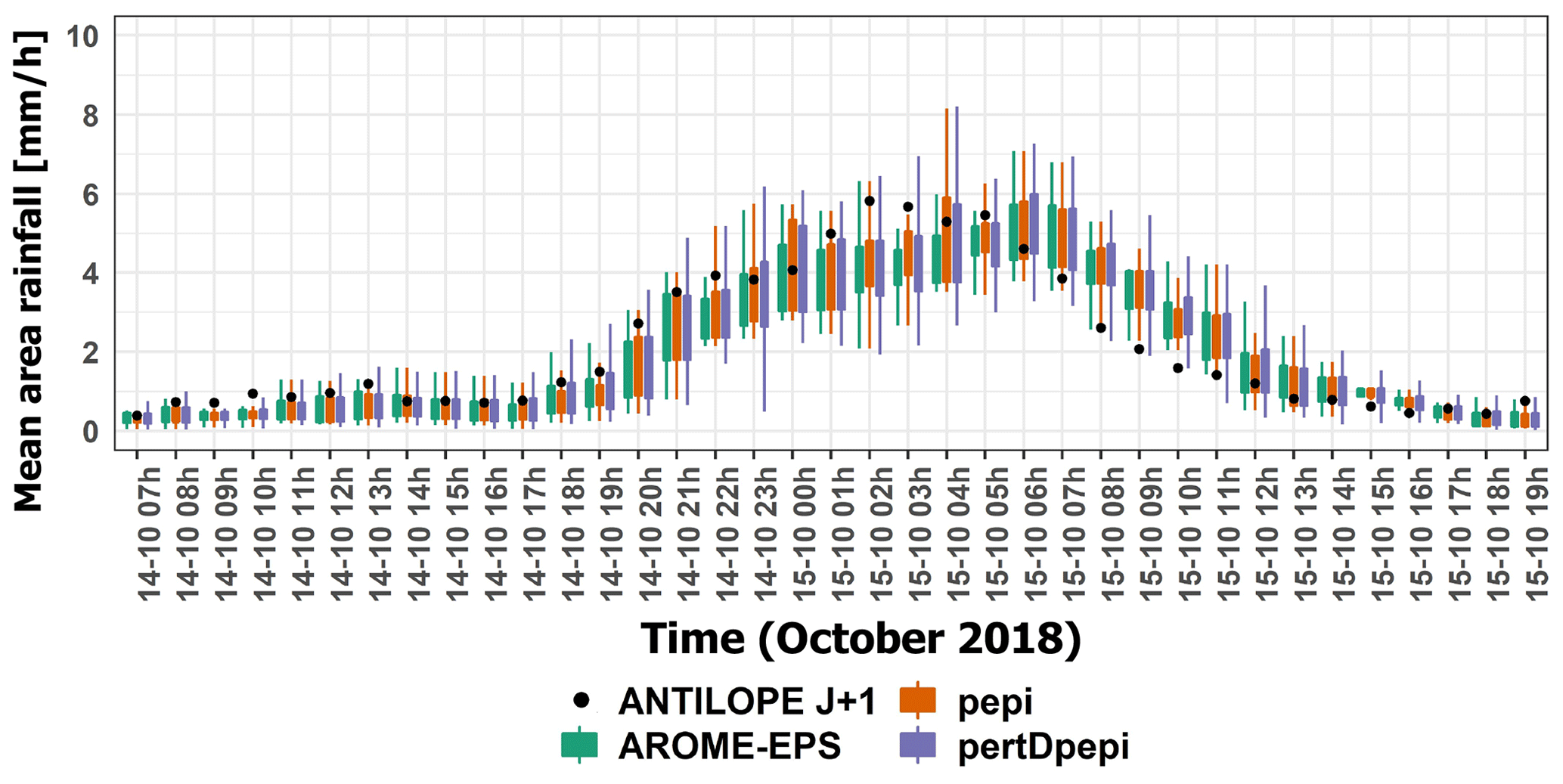
Figure A2 Temporal evolution of observed hourly rainfall rates (black dots) and 6 h lead time ensemble forecasts (boxplots) during the October 2018 flood event. Rainfall rates are averaged over the Aude River basin (6074 km²). The boxplots correspond to AROME-EPS (green), pepi (orange) and pertDpepi (purple). Whiskers reflect the min–max range and boxes the inter-percentile (25th–75th) for the forecasts.

A2 Comparison of observed and forecast rainfall amounts over 15 h for the 1 and 6 h lead times

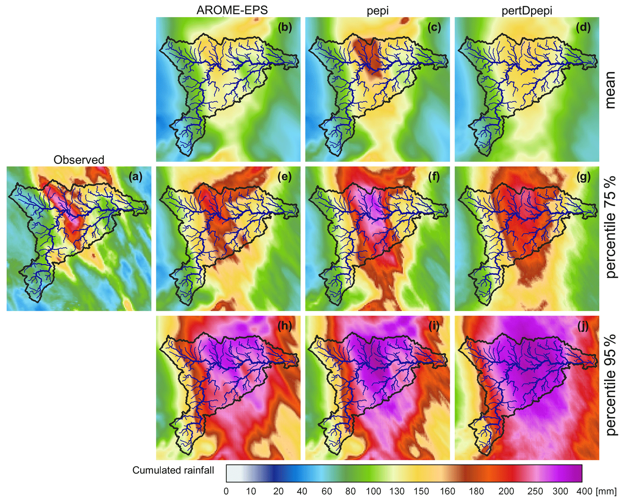
Figure A3 Comparison of observed and forecast (1 h lead time) rainfall amounts over 15 h (from 14 October at 20:00 UTC to 15 October at 11:00 UTC): (a) observed rainfall, (b, e, h) AROME-EPS ensemble mean and 75th and 95th percentiles, (c, f, i) pepi ensemble mean and 75th and 95th percentiles, and (d, g, j) pertDpepi ensemble mean and 75th and 95th percentiles.

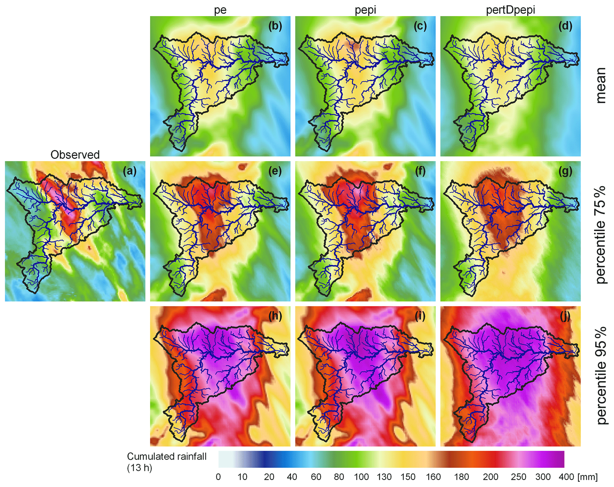
Figure A4 Comparison of observed and forecast (6 h lead time) rainfall amounts over 15 h (from 14 October at 20:00 UTC to 15 October at 11:00 UTC): (a) observed rainfall, (b, e, h) AROME-EPS ensemble mean and 75th and 95th percentiles, (c, f, i) pepi ensemble mean and 75th and 95th percentiles, and (d, g, j) pertDpepi ensemble mean and 75th and 95th percentiles.

A3 Rank diagrams for the 1 and 6 h lead time rainfall forecasts

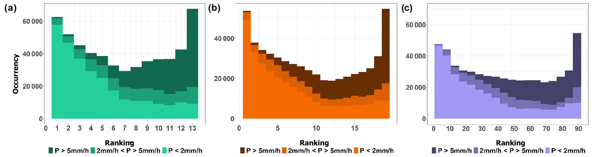
Figure A5 Rank diagrams of the three ensemble rainfall forecast products for rainfall rates under 2 mm h⁻¹, between 2 and 5 mm h⁻¹, and above 5 mm h⁻¹ and for a lead time of 1 h: (a) AROME-EPS, (b) pepi and (c) pertDpepi.

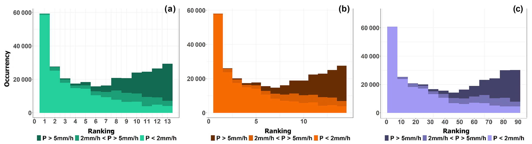
Figure A6 Rank diagrams of the three ensemble rainfall forecast products for rainfall rates under 2 mm h⁻¹, between 2 and 5 mm h⁻¹, and above 5 mm h⁻¹ and for a lead time of 6 h: (a) AROME-EPS, (b) pepi and (c) pertDpepi.

Appendix B: Methodology used for the evaluation of discharge threshold anticipation with hydrological ensemble forecasts

The methodology used to evaluate the anticipation of the exceedances of selected discharge thresholds was directly inspired by the principle of the ROC curves method developed by Mason (1982) and Wilks (2011). The ROC curve (receiver operating characteristic) is a criterion evaluating the capacity of a forecasting system to detect the occurrence (reciprocally the non-occurrence) of an event. In hydrology, the event generally corresponds to the exceedance of a discharge threshold, and the ROC curve is generally built to summarize long time series of forecasts at one single basin outlet. Comparing at each time step the respective position of the forecast (for a given probability and a fixed lead time), the reference observation or simulation and the considered discharge threshold allow us to calculate the probability of detection (POD) and the false alarm rate (FAR) (Wilks, 2011; Jolliffe and Stephenson, 2012). The ROC curve is then plotted by using the pairs of points (FAR and POD) corresponding to different forecast probabilities.

In this study, the conventional computation of a ROC curve was adapted following the idea to focus the analysis on the first exceedance of a selected alert discharge threshold at the event temporal and geographical scales. This led us to introduce the following evolutions.

• All the ungauged outlets located in the HFA (1174 in this study) are considered to build the contingency table. For this purpose, hydrographs simulated with observed rainfall are used as reference hydrographs (RS hydrographs hereafter), and the discharge thresholds are adapted at each outlet based on a given return period.

• Only one unique time step for each outlet is considered, i.e., the first time at which the RS hydrograph exceeds the considered threshold or the time of the peak of the RS hydrograph in the case of no threshold exceedance. The use of many outlets (1174 in this study) compensates for the small number of considered time steps for the elaboration of the ROC curves.

• All the forecasts delivered before and covering the considered time step are merged to evaluate the anticipation and detection of the threshold exceedance without considering a unique lead time. In practice, we consider that a threshold exceedance is forecasted if at least one of the merged forecast hydrographs exceeds the threshold. This neighborhood method is in line with the methods discussed in Schwartz and Sobash (2017), the difference being that here it is a temporal neighborhood by max function that is considered.

According to these general principles, for a given forecast probability, the contingency table is obtained in the following way.

• If the threshold is exceeded by the RS hydrograph (Fig. B1), the date (day and hour) of the first exceedance is identified. All the runs of forecasts issued before and covering this date are then selected (i.e., six runs here according to the maximum forecast lead time of 6 h and the 1 h time step between successive runs). A hit is counted in the contingency table if at least one of the six runs exceeds the discharge threshold at any lead time (Fig. B1a), and a miss is counted if none of the six hydrological forecasts exceed the threshold at any lead time (Fig. B1b).

• In the case the discharge threshold is not exceeded by the RS hydrograph (Fig. B2), the date of the peak discharge of the RS hydrograph is first identified. The runs of forecasts issued before and covering this date are then selected. Again, a false alarm is counted if at least one of the selected runs exceeds the discharge threshold at any lead time (Fig. B2a) and a correct rejection if none of the selected runs exceed the discharge threshold at any lead time (Fig. B2b)

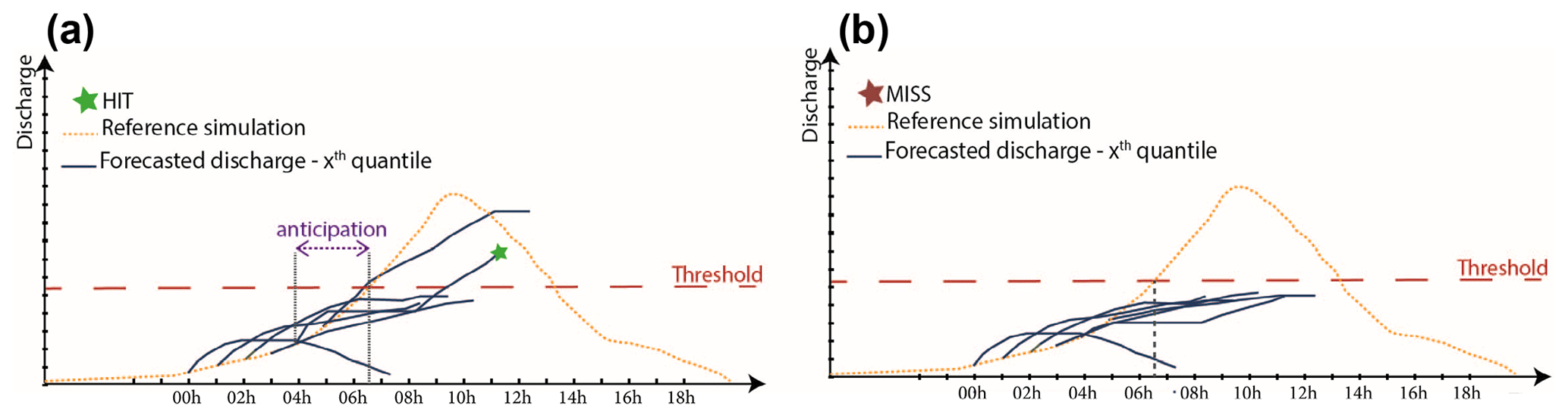
Figure B1 Illustration of the discharge threshold exceedance detection method: (a) hit case and (b) miss. The way the anticipation is computed is also illustrated (time difference between the time the discharge threshold is exceeded for the RS hydrograph and the time of the first run which detects the exceedance).

Each contingency table finally contains as many values (hit, misses, false alarms, correct rejection) as the number of outlets in the HFA. The ROC curve can then be drawn by deriving the POD and FAR scores from the contingency tables, following the traditional way described above. An advantage of this way of building contingency tables is that each table can be presented on a map by drawing the evaluation obtained at each outlet or sub-basin (hit, miss, false alarm or correct rejection). This allows us to easily analyze how the ensemble forecasts performed geographically according to these criteria.

Additionally, for each hit entry of the contingency tables, the anticipation time can also be evaluated (Fig. B1a). It corresponds to the difference between (i) the time of exceedance of the discharge threshold by the RS hydrograph and (ii) the time of the first forecast run that detects a threshold exceedance. We can thus draw the distribution of the anticipation times obtained over the considered outlets for the different percentiles and ensemble forecast.

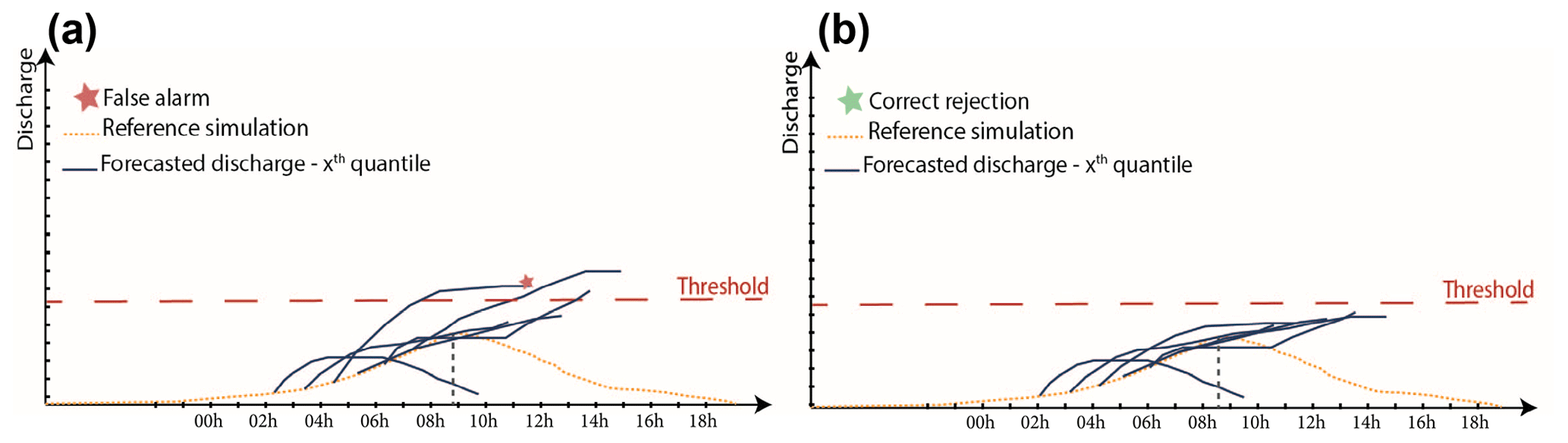
Figure B2 Illustration of the discharge threshold exceedance detection method: (a) false alarm case and (b) correct rejection.

Appendix C: Forecast hydrographs obtained for AROME-EPS for 3 h lead times

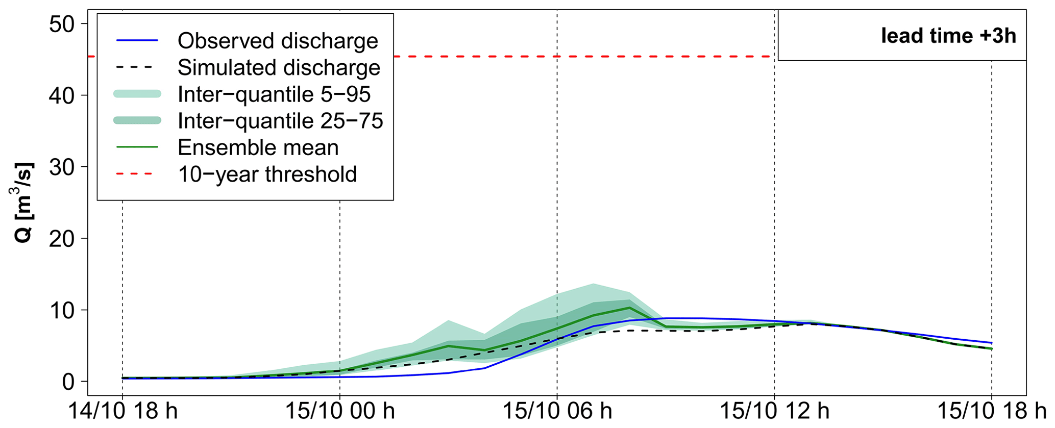
Figure C1 Detailed hydrological 3 h lead time forecast evaluation at outlet 1 for AROME-EPS. In blue, the observed discharge at the gauging station.

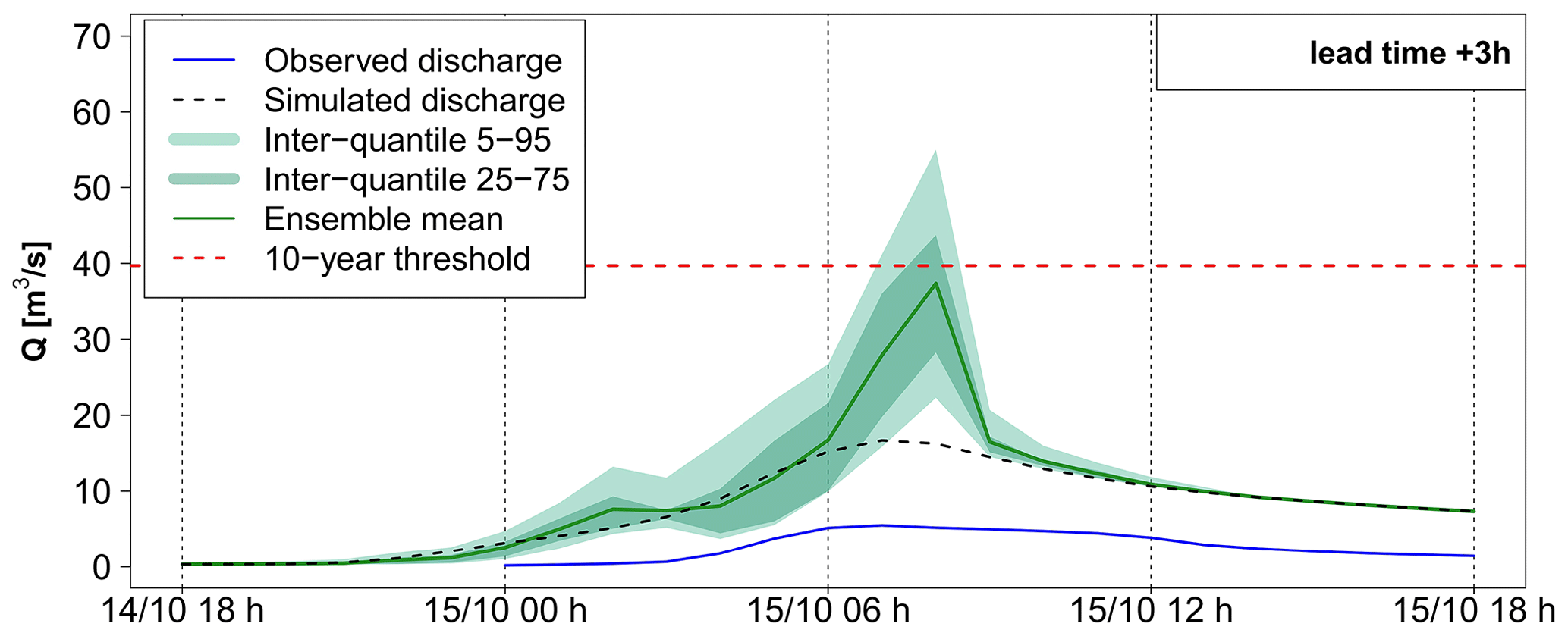
Figure C2 Detailed hydrograph for 3 h lead time forecast evaluation at outlet 2 for AROME-EPS. In blue, the observed discharge at the gauging station.

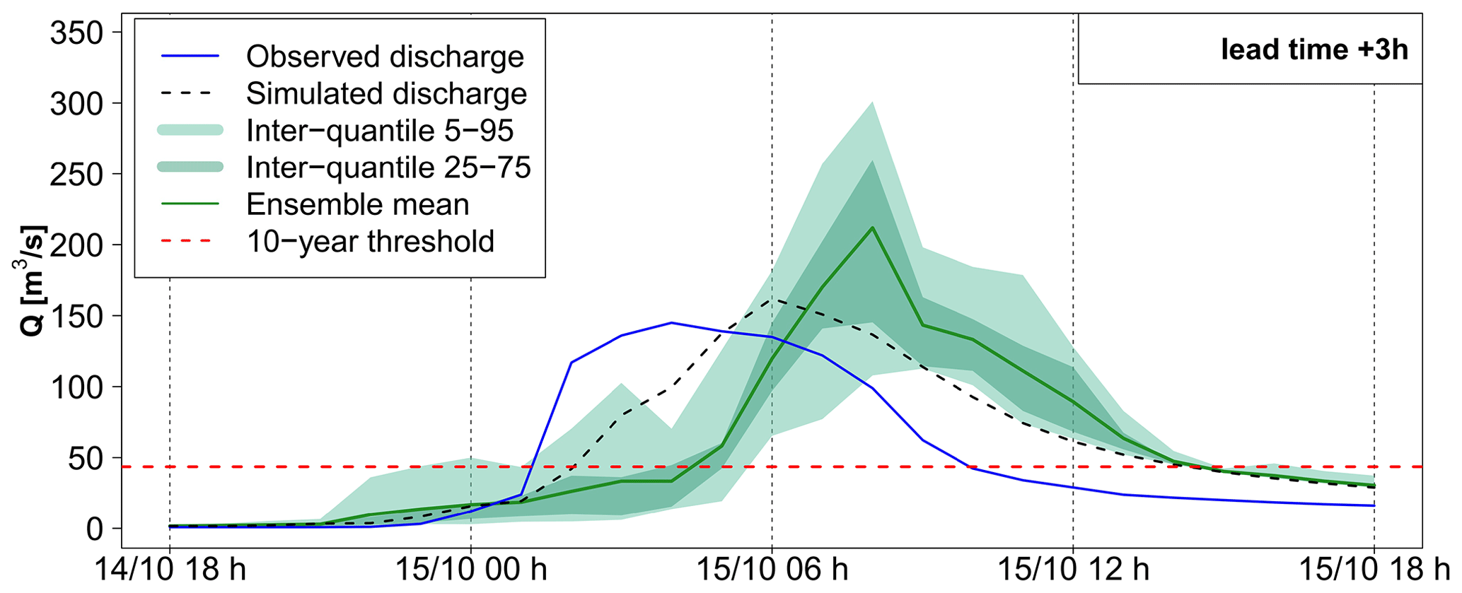
Figure C3 Detailed hydrograph for 3 h lead time forecast evaluation at outlet 3 for AROME-EPS. In blue, the observed discharge at the gauging station.

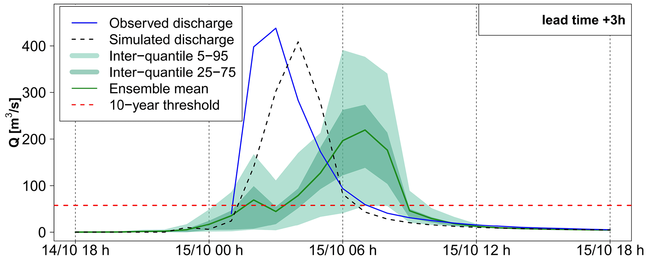
Figure C4 Detailed hydrograph for 3 h lead time forecast evaluation at outlet 4 for AROME-EPS. In blue, the observed discharge at the gauging station.

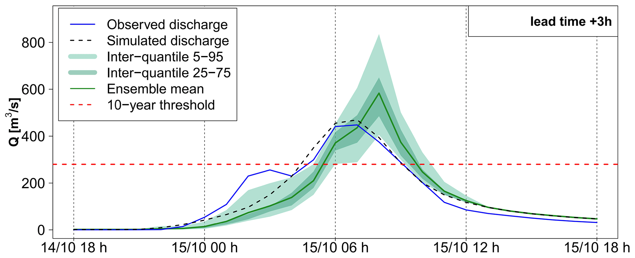
Figure C5 Detailed hydrograph for 3 h lead time forecast evaluation at outlet 5 for AROME-EPS. In blue, the observed discharge at the gauging station.

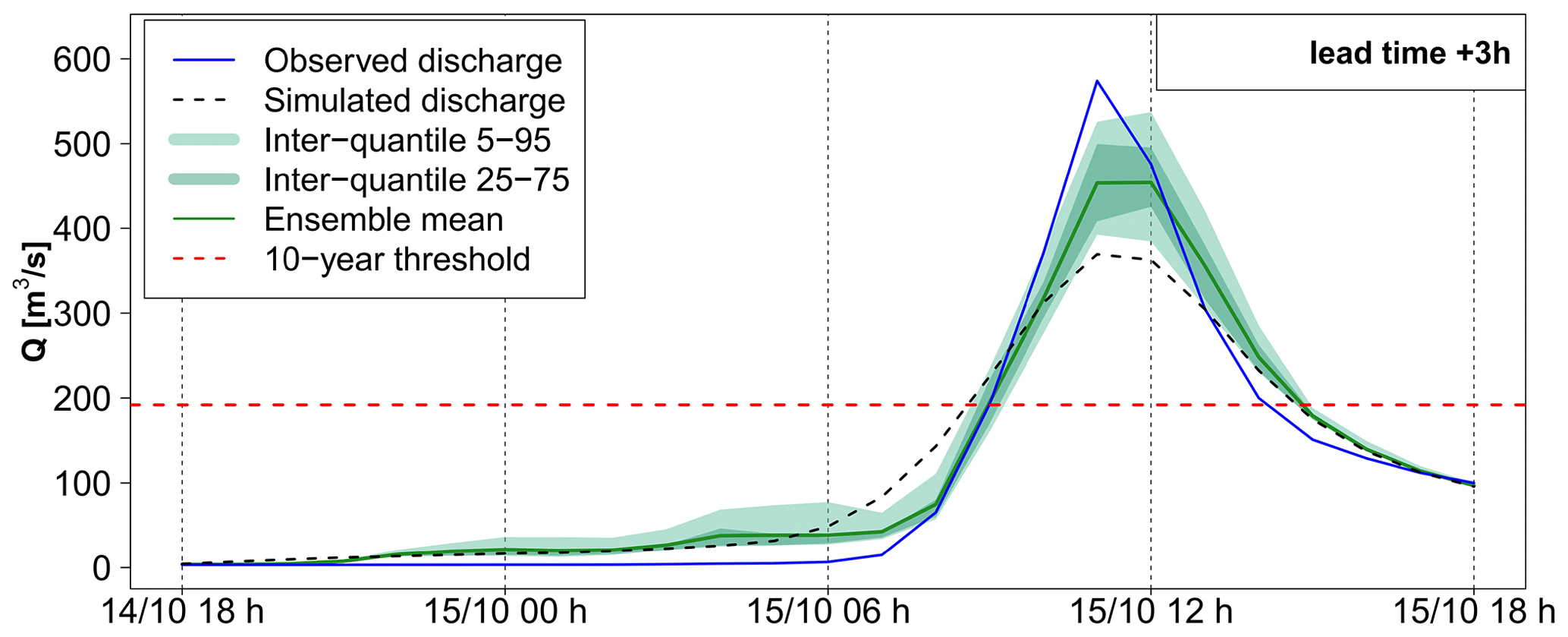
Figure C6 Detailed hydrograph for 3 h lead time forecast evaluation at outlet 6 for AROME-EPS. In blue, the observed discharge at the gauging station.

Appendix D: Spread–skill relationship and forecast hydrographs obtained for 6 h lead times

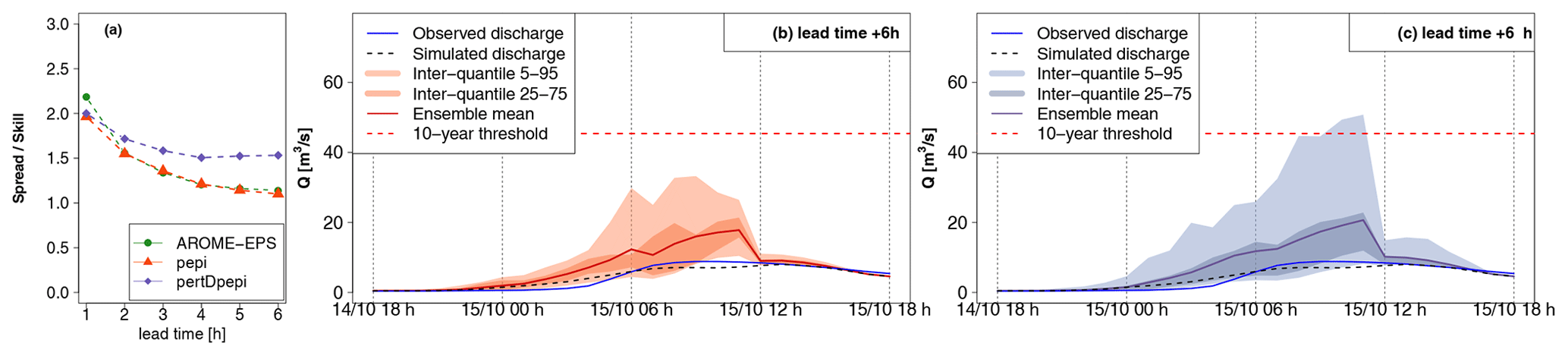
Figure D1 Detailed hydrological forecast evaluation at outlet 1 (216 km²): (a) spread–skill relationship, (b) hydrographs of 6 h lead time forecasts with pepi and (c) hydrographs of 6 h lead time forecasts with pertDpepi. In blue, the observed hydrograph at the gauging station.

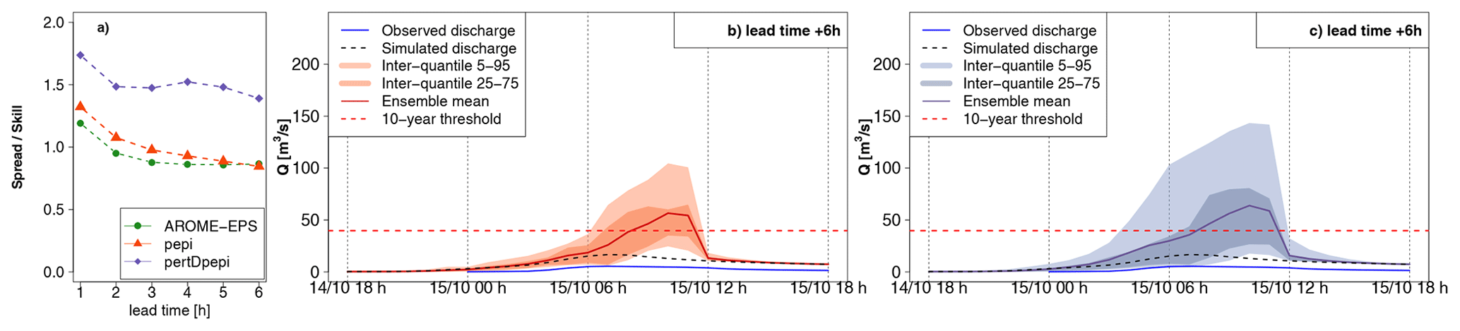
Figure D2 Detailed hydrological forecast evaluation at outlet 2 (197 km²): (a) spread–skill relationship, (b) hydrographs of 6 h lead time forecasts with pepi and (c) hydrographs of 6 h lead time forecasts with pertDpepi. In blue, the observed hydrograph at the gauging station.

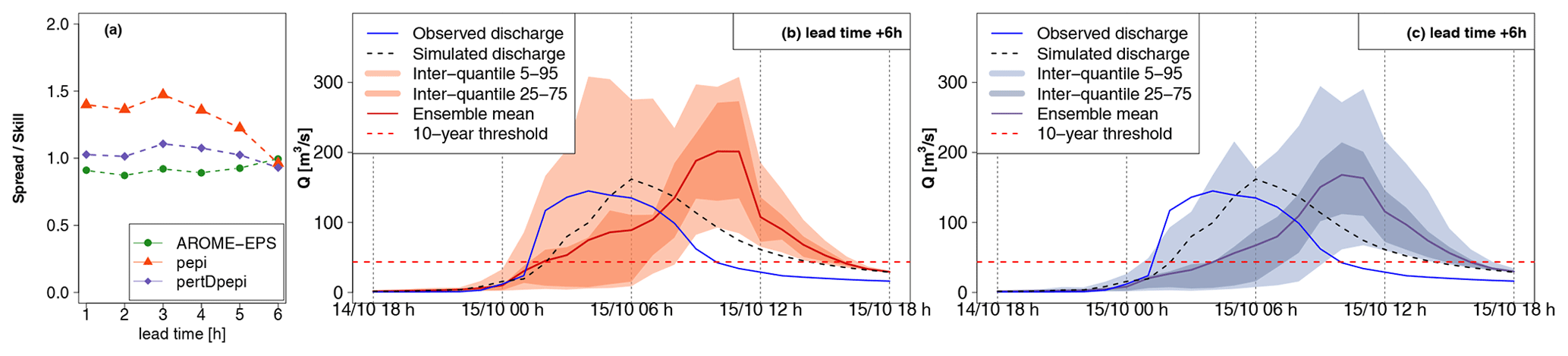
Figure D3 Detailed hydrological forecast evaluation at outlet 3 (85 km²): (a) spread–skill relationship, (b) hydrographs of 6 h lead time forecasts with pepi and (c) hydrographs of 6 h lead time forecasts with pertDpepi. In blue, the observed hydrograph at the gauging station.

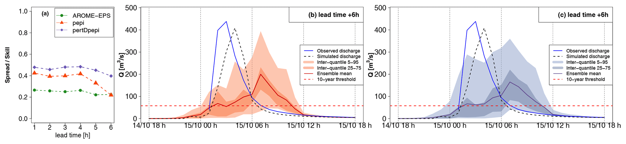
Figure D4 Detailed hydrological forecast evaluation at outlet 4 (173 km²): (a) spread–skill relationship, (b) hydrographs of 6 h lead time forecasts with pepi and (c) hydrographs of 6 h lead time forecasts with pertDpepi. In blue, the observed hydrograph at the gauging station.

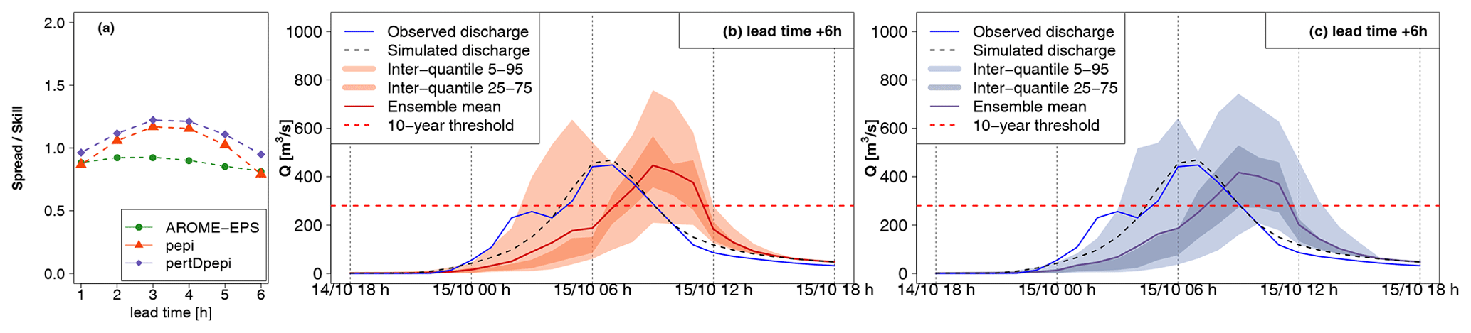
Figure D5 Detailed hydrological forecast evaluation at outlet 5 (263 km²): (a) spread–skill relationship, (b) hydrographs of 6 h lead time forecasts with pepi and (c) hydrographs of 6 h lead time forecasts with pertDpepi. In blue, the observed hydrograph at the gauging station.

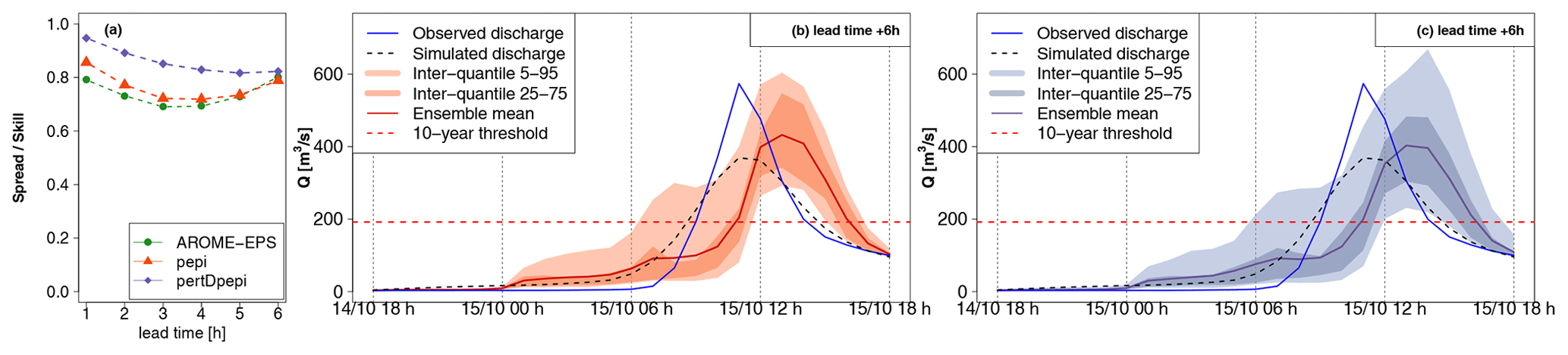
Figure D6 Detailed hydrological forecast evaluation at outlet 6 (257 km²): (a) spread–skill relationship, (b) hydrographs of 6 h lead time forecasts with pepi and (c) hydrographs of 6 h lead time forecasts with pertDpepi. In blue, the observed hydrograph at the gauging station.