Earthquake hazard characterization by using entropy: application to northern Chilean earthquakes

The mechanical description of the seismic cycle has an energetic analogy in terms of statistical physics and the second law of thermodynamics. In this context, an earthquake can be considered a phase transition, where continuous reorganization of stresses and forces reflects an evolution from equilibrium to non-equilibrium states, and we can use this analogy to characterize the earthquake hazard of a region. In this study, we used 8 years (2007–2014) of high-quality Integrated Plate Boundary Observatory Chile (IPOC) seismic data for > 100 000 earthquakes in northern Chile to test the theory that Shannon entropy, H, is an indicator of the equilibrium state of a seismically active region. We confirmed increasing H reflects the irreversible transition of a system and is linked to the occurrence of large earthquakes. Using variation in H, we could detect major earthquakes and their foreshocks and aftershocks, including the 2007 M_w 7.8 Tocopilla earthquake, the 2014 M_w 8.1 Iquique earthquake, and the 2010 and 2011 Calama earthquakes (M_w 6.6 and 6.8, respectively). Moreover, we identified possible periodic seismic behaviour between 80 and 160 km depth.

1 Introduction

The seismicity of a region contains abundant information that can be used from different points of view, attempting to know when an earthquake is going to occur. In physics, entropy is one of the most fascinating, abstract and complex concepts. The present paper shows how to use entropy to characterize the occurrence of earthquakes, i.e. to have a characterization of the seismic hazard in entropic terms.

It is well known (e.g. Nikulov, 2022) that the second law of thermodynamics postulates the existence of irreversible processes in physics: the total entropy of an isolated system can increase but cannot decrease. Namely, only those phenomena for which the entropy of the universe increases are allowed. Thus, in seismology, it is natural to use entropy to find out future states that a region of the Earth's crust can access from its current state (Akopian, 2015).

The concept of entropy and its connection to the second law of thermodynamics was proposed by Clausius in 1865 (Clausius, 1865), and a few years later, Boltzmann realized that entropy could be used to connect the microscopic motion of particles to the macroscopic world; in his analysis, entropy (S) is proportional to the number of accessible micro states of the system (Ω) and is expressed by the famous Boltzmann equation:

$$\begin{array}{}\text{(1)}& S=k\ln \mathrm{\Omega },\end{array}$$

where k is Boltzmann's constant. Ben-Naim (2020) stated that at first glance, Boltzmann's entropy and Clausius' entropy are absolutely different; however, there is complete agreement in calculating changes in entropy using the two methods (up to a multiplicative constant). The generalization of Boltzmann's entropy for systems described by other macroscopic variables corresponded to Gibbs (Zupanovic and Domagoj, 2018) and can be written as

$$\begin{array}{}\text{(2)}& S=-k\sum _{i=\mathrm{1}}^{\mathrm{\Omega }}{p}_i\log p_i,\end{array}$$

where p_i is the probability of the system being in the ith state. Shannon (1948) and Shannon and Weaver (1949) introduced Boltzmann–Gibbs's entropy concept to communication theory and defined the measure of information as

$$\begin{array}{}\text{(3)}& I\left(p\right)=\sum _{i=\mathrm{1}}^{\mathrm{\Omega }}{p}_i\log p_i,\end{array}$$

where p is the distribution of states, and p_i is the relative frequency for each event i. The function I(p) is called “Shannon information” because it is a measure of knowledge; therefore, −I(p) denotes a lack of knowledge or ignorance as Majewski (2001) has highlighted. Clearly, I(p) is always negative or 0. As such, it is possible to define the “Shannon information entropy” (H) as the negative information measure (Ben-Naim, 2017); that is

$$\begin{array}{}\text{(4)}& H\left(p\right)=-I\left(p\right)=-\sum _{i=\mathrm{1}}^{\mathrm{\Omega }}{p}_i\log p_i,\end{array}$$

which is always positive or 0. In the last equation it has been assumed, for simplicity (Truffet, 2018), that k = 1, or equivalently, that $H\left(p\right)=-I\left(p\right)/k$. Some (relatively) recent research carried out in the field of information theory suggests that the above expressions can be generalized. Thus, Tsallis (1988) proposed the use of

$$\begin{array}{}\text{(5)}& S_{\mathit{\tau }}={\displaystyle \frac{k}{\mathit{\tau }-\mathrm{1}}}\left(\mathrm{1}-\sum _{i=\mathrm{1}}^{\mathrm{\Omega }}{p}_i^{\mathit{\tau }}\right),\end{array}$$

where τ is called the entropic index and can, in principle, be any real number. The standard distribution that characterizes Boltzmann–Gibbs statistics is a particular case of Tsallis entropy in the limit of τ = 1. Other generalizations, such as Rényi entropy, can be found in the scientific literature (e.g. Majewski and Teisseyre, 1997).

From the point of view of classical thermodynamics (Varotsos et al., 2011; Vargas et al., 2015; Sarlis et al., 2008; Vogel et al., 2020; Telesca et al., 2022; Varotsos et al., 2022), but also statistical mechanics (Michas et al., 2013; Vallianatos et al., 2015; Papadakis et al., 2015; Vallianatos et al., 2016, 2018), variation in entropy has been widely used in seismology as an indicator of the evolution of a system (from precursor papers such as Rundle et al., 2003, or Sornette and Werner, 2009, to recent ones from Posadas et al., 2021; Pasten et al., 2022; or Posadas and Sotolongo-Costa, 2023).

In this paper, we used 8 years (2007–2014) of high-quality Integrated Plate Boundary Observatory Chile (IPOC) seismic data for > 100 000 earthquakes in northern Chile to test the theory that Shannon entropy, H, is an indicator of the equilibrium state of a seismically active region. Moreover, we will rough out a thermodynamics vision of the seismic cycle to characterize the seismic hazard of the northern Chilean seismicity.

2 Methods

2.1 Theoretical framework

Let us start with a representation of the state of a given seismically active region from the distribution of earthquakes with magnitudes M associated with time t, that is, P(M). Thus, entropy, H, postulated by Shannon, which is associated with information flow, can be reformulated (De Santis et al., 2019) as

$$\begin{array}{}\text{(6)}& H\left(t\right)=-\underset{M_{\mathrm{0}}}{\overset{M_{max}}{\int }}P\left(M\right)\cdot \log \left(P\right(M\left)\right)\mathrm{d}M,\end{array}$$

where M₀ is the threshold magnitude (i.e. the magnitude for which the seismic catalogue is complete), and M_max is the maximum magnitude up to which earthquakes occur. There are two restrictive conditions to solve that integral. First

$$\begin{array}{}\text{(7)}& \underset{M_{\mathrm{0}}}{\overset{M_{max}}{\int }}P\left(M\right)\mathrm{d}M=\mathrm{1}.\end{array}$$

The second arises from the fact that the average value of all possible magnitudes $\stackrel{\mathrm{‾}}{M}$, in a certain period, is

$$\begin{array}{}\text{(8)}& \stackrel{\mathrm{‾}}{M}=\underset{M_{\mathrm{0}}}{\overset{M_{max}}{\int }}M\cdot P\left(M\right)\mathrm{d}M.\end{array}$$

The second law of thermodynamics requires that there exists a distribution under which H would be at its maximum value while under the two restrictive conditions; that is, the spontaneous development of the system from a state of non-equilibrium to a state of equilibrium is a process in which entropy increases, and the final state of equilibrium corresponds to the maximum entropy. Thus, the problem can be solved by applying the Lagrange multiplier method; to do that, we define the Lagrangian L as

$$\begin{array}{}\text{(9)}& \begin{array}{rl}L\left(P\left(M\right)\right)& =H\left(P\left(M\right)\right)-{\mathit{\lambda }}_{\mathrm{1}}\underset{M_{\mathrm{0}}}{\overset{M_{max}}{\int }}P\left(M\right)\mathrm{d}M\\ & -{\mathit{\lambda }}_{\mathrm{2}}\underset{M_{\mathrm{0}}}{\overset{M_{max}}{\int }}MP\left(M\right)\mathrm{d}M,\end{array}\end{array}$$

where λ₁ and λ₂ are Lagrange's multipliers; then, it is possible to deduce the probability density function in the form (Feng and Luo, 2009)

$$\begin{array}{}\text{(10)}& P\left(M\right)={\displaystyle \frac{\mathrm{1}}{\stackrel{\mathrm{‾}}{M}-M_{\mathrm{0}}}}\exp \left(-{\displaystyle \frac{M-M_{\mathrm{0}}}{\stackrel{\mathrm{‾}}{M}-M_{\mathrm{0}}}}\right).\end{array}$$

On the other hand, if we have N earthquakes and n denotes the number of earthquakes with magnitudes equal to or larger than M,

$$\begin{array}{}\text{(11)}& P\left(M\right)={\displaystyle \frac{n}{N}};\end{array}$$

then, we match both formulas and take logarithms to get

$$\begin{array}{}\text{(12)}& \log n=\log \left({\displaystyle \frac{N}{\stackrel{\mathrm{‾}}{M}-M_{\mathrm{0}}}}\right)+{\displaystyle \frac{M_{\mathrm{0}}\cdot \log \left(e\right)}{\stackrel{\mathrm{‾}}{M}-M_{\mathrm{0}}}}-{\displaystyle \frac{\log \left(e\right)}{\stackrel{\mathrm{‾}}{M}-M_{\mathrm{0}}}}\cdot M.\end{array}$$

But, the Gutenberg–Richter relationship (Gutenberg and Richter, 1944) states that the distribution of earthquake magnitudes follows an empirical and universal relationship:

$$\begin{array}{}\text{(13)}& \log n=a-bM,\end{array}$$

where n is the cumulative number of earthquakes with a magnitude equal to or larger than M, and a and b are real constants that may vary in space and time. Parameter a characterizes the general level of seismicity in a given area during the study period (i.e. the higher the a value, the higher the seismicity), whereas parameter b, which is typically close to 1, describes the relative abundance of large to smaller shocks. Now, identifying terms from Eqs. (12) and (13), we obtain

$$\begin{array}{}\text{(14)}& a=\log \left({\displaystyle \frac{N}{\stackrel{\mathrm{‾}}{M}-M_{\mathrm{0}}}}\right)+{\displaystyle \frac{M_{\mathrm{0}}\cdot \log \left(e\right)}{\stackrel{\mathrm{‾}}{M}-M_{\mathrm{0}}}}\end{array}$$

and

$$\begin{array}{}\text{(15)}& b={\displaystyle \frac{\log \left(e\right)}{\stackrel{\mathrm{‾}}{M}-M_{\mathrm{0}}}}.\end{array}$$

Hence, the probability density function (Eq. 10) can be rewritten as

$$\begin{array}{}\text{(16)}& P\left(M\right)={\displaystyle \frac{b}{\log \left(e\right)}}\cdot {\mathrm{10}}^{-b(M-M_{\mathrm{0}})},\end{array}$$

and, finally, substituting into Eq. (6), we get (De Santis et al., 2011)

$$\begin{array}{}\text{(17)}& \begin{array}{rl}H& =-\underset{M_{\mathrm{0}}}{\overset{\mathrm{\infty }}{\int }}{\displaystyle \frac{b\cdot {\mathrm{10}}^{-b\left(M-M_{\mathrm{0}}\right)}}{\log \left(e\right)}}\cdot \log \left({\displaystyle \frac{b\cdot {\mathrm{10}}^{-b\left(M-M_{\mathrm{0}}\right)}}{\log \left(e\right)}}\right)\mathrm{d}M\\ & =-\log \left(b\right)+\log \left(e\cdot \log \left(e\right)\right).\end{array}\end{array}$$

After computing b from the classical Utsu expression (Utsu, 1965)

$$\begin{array}{}\text{(18)}& b={\displaystyle \frac{\log \left(e\right)}{\stackrel{\mathrm{‾}}{M}-\left(M_{\mathrm{0}}-\frac{\mathrm{\Delta }M}{\mathrm{2}}\right)}},\end{array}$$

where ΔM is the resolution of magnitude (usually ΔM=0.1), and the value of entropy can be found.

2.2 Methodology

Our analysis approach included three steps:

1. First, the value of the threshold magnitude (M₀) is a critical choice. There are two main classes of methods to evaluate M₀: catalogue-based methods (e.g. Amorèse, 2007) and network-based methods (e.g. D'Alessandro et al., 2011). We used a catalogue-based method because the necessary inputs were available from our dataset. Although some studies estimate the value of M₀ by fitting the linear Gutenberg–Richter relationship to the observed frequency–magnitude distribution (the magnitude at which the lower end of the frequency–magnitude distribution departs from the Gutenberg–Richter relationship is taken as M₀; Zúñiga and Wyss, 1995), several other methods can better determine the threshold magnitude. Catalogue-based techniques include day-to-night noise modulation (day/night method) (Rydele and Sacks, 1989), the entire magnitude range (Ogata and Katsura, 1993), the maximum curvature (MAXC) technique or goodness-of-fit test (GFT) (Wiemer and Wyss, 2000), b-value stability (MBS) (Cao and Gao, 2002), and median-based analysis of the segment slope (MBASS) (Amorèse, 2007). The MAXC technique is mainly used in applied techniques and was chosen here; however, the results do not differ significantly among these approaches.

2. Second, the time interval W was determined for the calculation of entropy (Eq. 17) using the minimum number of earthquakes to calculate H. The time interval can be chosen by defining a cumulative, moving or overlapping earthquake window. Here, the results are presented for a sliding window to avoid the memory effect. It turns out that the results are substantially the same regardless of the approach taken. On the whole, the final window size offered a reasonable compromise between resolution and smoothing. The width of the window was chosen by following the approach of De Santis et al. (2011), which is based on meaningful values of b. In short, 200 events are the minimum needed to perform a robust statistical estimation of b and H. This has been confirmed by previous statistical analyses of a and b values (Utsu, 1999). However, larger values of W can be adopted depending on the relative error when entropy is computed (Posadas et al., 2021); this criterion is explained below in the Results section.

3. Finally, the entropy function was obtained for each time t following Eq. (17). By convention, the time attributed to each point of the analyses was the time of the last seismic event considered in each window. The occurrence of a large earthquake (or the accumulation of several important ones) is expected to lead the seismic system to a state of greater disorder. Then, any earthquake is an irreversible transition to a new state carrying an increase in entropy. Once the major shock is over, entropy returns to stable values.

3 Data: the northern Chilean seismicity

The Pacific Ring of Fire, a 40 000 km horseshoe marking the tectonic boundaries of the Pacific Ocean (primarily along the boundaries of the Pacific Plate), hosts 90 % of Earth's seismic activity and 75 % of the active volcanoes. Also known as the Circum-Pacific Belt, it extends from Tonga and the New Hebrides islands through Indonesia, the Philippines, Japan, the Kuril Islands and the Aleutian Islands to the western coast of North America, before ending in the Cordillera de los Andes of South America. Among these regions, the northern Chile forearc experiences abundant interplate and intraplate earthquakes, intermediate and deep earthquakes associated with subduction, and a high tsunami risk along coastal areas. Events such as the 2007 M_w 7.8 Tocopilla earthquake (Delouis et al., 2009), 2010 M_w 8.8 Maule megathrust earthquake (Derode et al., 2021) and 2014 M_w 8.1 Iquique earthquake (Cesca et al., 2016) highlight the special relevance of this region. As such, monitoring seismic and volcanic activity in northern Chile using dense seismic networks (permanent and temporary) to create extensive high-quality seismic catalogues is a priority. To this end, the Integrated Plate Boundary Observatory Chile (IPOC), established by a network of European and South American institutions, operates a wide system of instruments and projects dedicated to the study of earthquakes and deformation at the continental margin of Chile (https://www.ipoc-network.org/, last access: July 2022). The network extends from the Peru–Chile border in the north to the city of Antofagasta in the south and from the coast in the west to the high Andes in the east.

In this study, we used high-quality IPOC data from 2007 to 2014 (the period for which data are publicly available) to test the theory that Shannon entropy (we will use Shannon entropy but whatever else such as Tsallis entropy, e.g. Vallianatos et al., 2015, 2018; Khordad et al., 2022; or Rastegar et al., 2022, could be adopted) represents an indicator of the equilibrium state of a seismically active region (or seismic system); we hypothesized that the relationship between increasing entropy and the occurrence of large earthquakes reflects the irreversible transition of a system. The data included records of 101 601 accurately located earthquakes within an epicentral area of 17–25^∘ S and 66–72^∘ W (Fig. 1a). A comprehensive study of the dataset can be found in Sippl et al. (2018a).

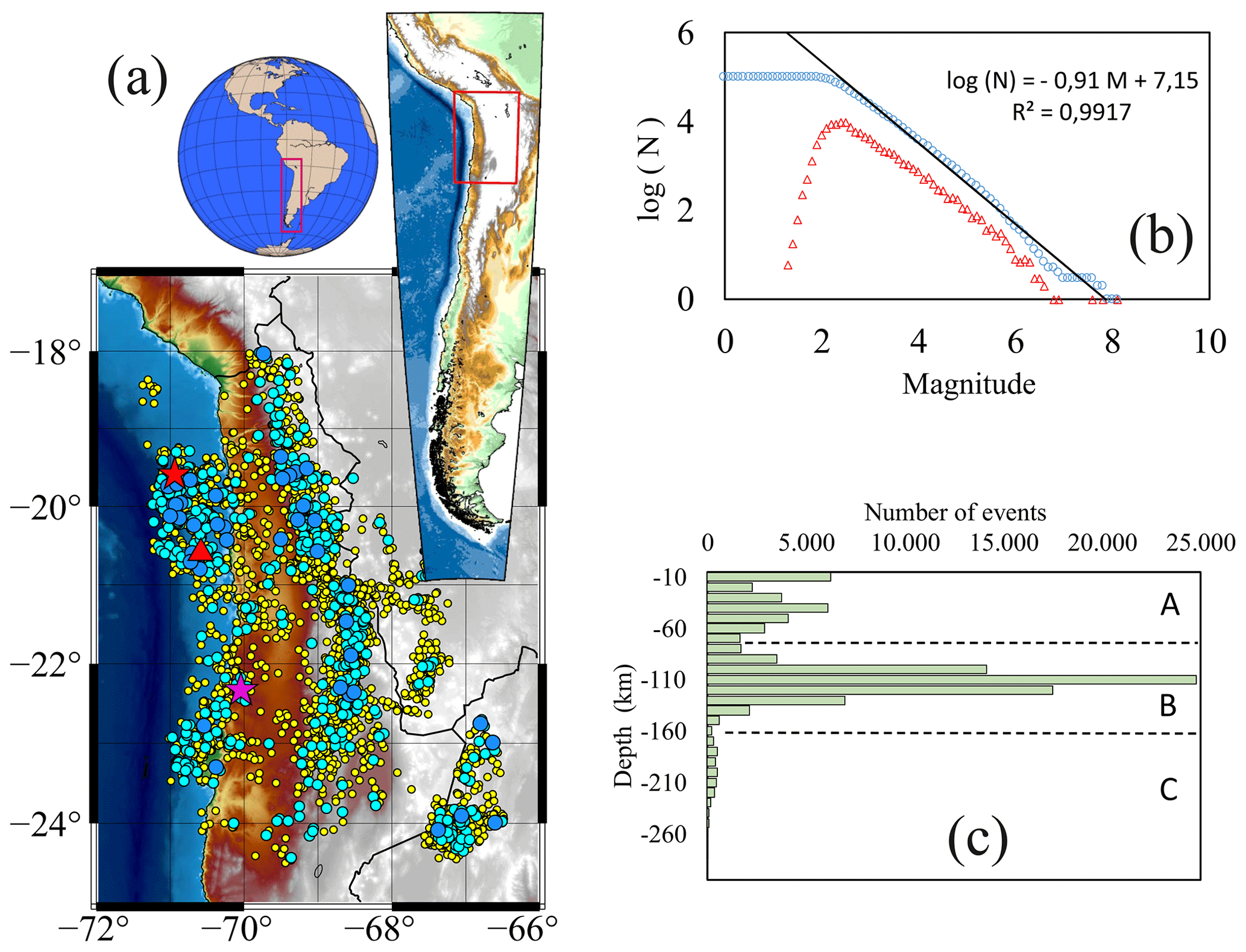
Figure 1 (a) Seismicity within an epicentral area of 17–25^∘ S and 66–72^∘ W between 2007 and 2014. Data are from the Integrated Plate Boundary Observatory Chile (IPOC) catalogue, which contains > 100 000 earthquakes; however, only events with magnitudes of > 4.0 are shown here (3960 events in total). Circle colours denote event magnitudes: yellow is 4.0–4.9, cyan is 5.0–5.9 and blue is 6.0–6.9. Earthquakes with magnitudes of > 7.0 include the 2007 M_w 7.8 Tocopilla earthquake (magenta star), 2014 M_w 8.1 Iquique earthquake (red star) and its main aftershock (M_w = 7.6, shown by the red triangle). (b) Gutenberg–Richter relationship. Blue circles denote the cumulative number of earthquakes; red triangles denote the non-cumulative number of earthquakes. Based on the maximum curvature (MAXC) technique (Wiemer and Wyss, 2000), M_w = 2.2. (c) Histogram of earthquake depth. Bins have a 10 km resolution, and three regions can be differentiated: zone A (up to 80 km depth), zone B (80–160 km depth) and zone C (> 160 km depth).​​​​​​​

4 Results

Earthquakes included in the catalogue have depths ranging from 0 to 300 km; it is evident that the seismic behaviour of the shallower part is different from that of the deeper zone, and so they should be analysed separately. However, first, we begin with a preliminary analysis of the whole catalogue to show whether the used technique could recognize earthquakes of greater magnitude. Subsequently, in a more detailed approach, a second analysis will be carried out that takes into account the depths (and, therefore, the different physical behaviours) associated with seismicity in each region.

Table 1 Earthquakes with magnitudes of > 6.5 in the Integrated Plate Boundary Observatory Chile (IPOC) catalogue for the period 2007 to 2014.

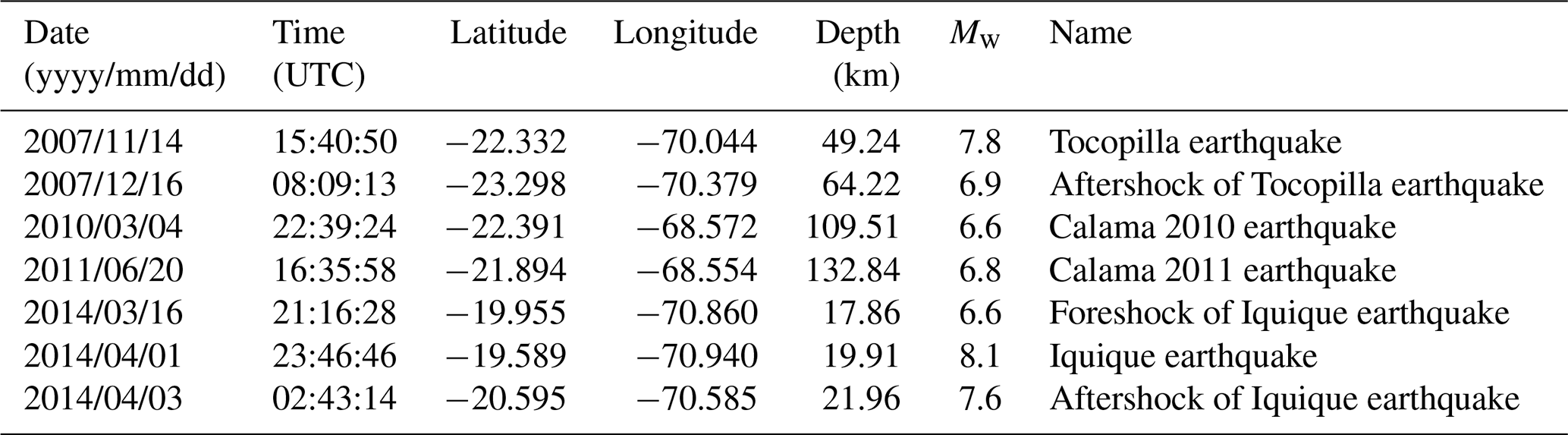
The seismic catalogue contains 32 earthquakes with magnitudes of 6.0 or greater, 7 of which have magnitudes of > 6.5 (Table 1). The two largest earthquakes are the M_w 7.8 Tocopilla earthquake (14 November 2007) and M_w 8.1 Iquique earthquake (1 April 2014). Figure 2 shows a time series of events for earthquakes with magnitudes of > 4.0; the number of earthquakes versus time is shown in Fig. 3.

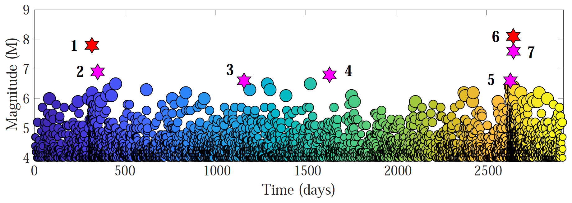
Figure 2 Magnitude versus time for earthquakes with magnitudes of > 4.0 within an epicentral area of 17–25^∘ S and 66–72^∘ W. Stars correspond to the earthquakes listed in Table 1, including the (1) 2007 M_w 7.8 Tocopilla earthquake, (2) 2007 M_w 6.9 Tocopilla aftershock, (3) 2010 M_w 6.6 Calama earthquake, (4) 2011 M_w 6.8 Calama earthquake, (5) M_w 6.6 foreshock of the Iquique earthquake, (6) M_w 8.1 Iquique earthquake and (7) M_w 7.6 aftershock of the Iquique earthquake. Circles' size increases gradually with magnitude and colour, from blue to yellow, highlighting the temporal evolution.

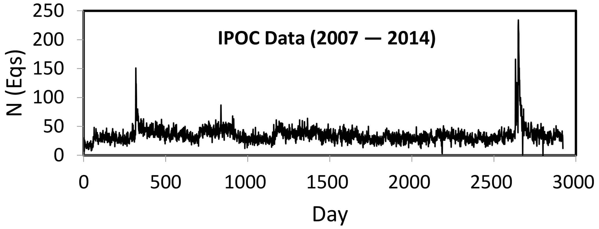
Figure 3 Number of daily earthquakes from 2007 to 2014 within an epicentral area of 17–25^∘ S and 66–72^∘ W. The seismic crises associated with the 2007 M_w 7.8 Tocopilla earthquake and 2014 M_w 8.1 Iquique earthquakes are clearly distinguished by the two prominent peaks.

First, the threshold magnitude M₀ is needed; to get it, we use the MAXC technique as we have mentioned before. Then, the Gutenberg–Richter relationship is obtained (Fig. 1b), and a value of M₀=2.2 is found.

The second step of our method is to determine the width of window W for the windowing process. Figure 4 shows the relative error of entropy versus window width. The choice of W must consider that values of b should be significant. One way to objectify this choice of W is to study the relative error when obtaining the entropy. Utsu's formalism (Utsu, 1965) showed that the uncertainty associated with the b value, interpreted as the error in the b value determination, is given by

$$\begin{array}{}\text{(19)}& \mathit{\sigma }={\displaystyle \frac{b}{\sqrt{N}}}.\end{array}$$

From Eqs. (17) and (19), it is easy to get that, for an entropy value H, the error margins are

$$\begin{array}{}\text{(20)}& \mathrm{\Delta }H=\log \left({\displaystyle \frac{b+\mathrm{\Delta }b}{b-\mathrm{\Delta }b}}\right).\end{array}$$

Hence, the relative error can be calculated as

$$\begin{array}{}\text{(21)}& \mathit{\epsilon }\left(\mathit{\%}\right)={\displaystyle \frac{\mathrm{100}}{H}}\cdot \log \left({\displaystyle \frac{b+\mathrm{\Delta }b}{b-\mathrm{\Delta }b}}\right).\end{array}$$

From Fig. 4, as the window width increases, the error decreases; when the window width is 4000 earthquakes (blue line), the error is barely 1 %. Overall, the relative errors of entropy range between 0.5 % and 2 % for window widths of > 500 cumulative earthquakes. From this point of view, the choice of W must be a reasonable compromise between calculated errors and the visibility of the results. We ultimately chose a window of W = 3000 earthquakes (yellow line), for which the relative error of entropy is close to 1 % and remains practically constant.

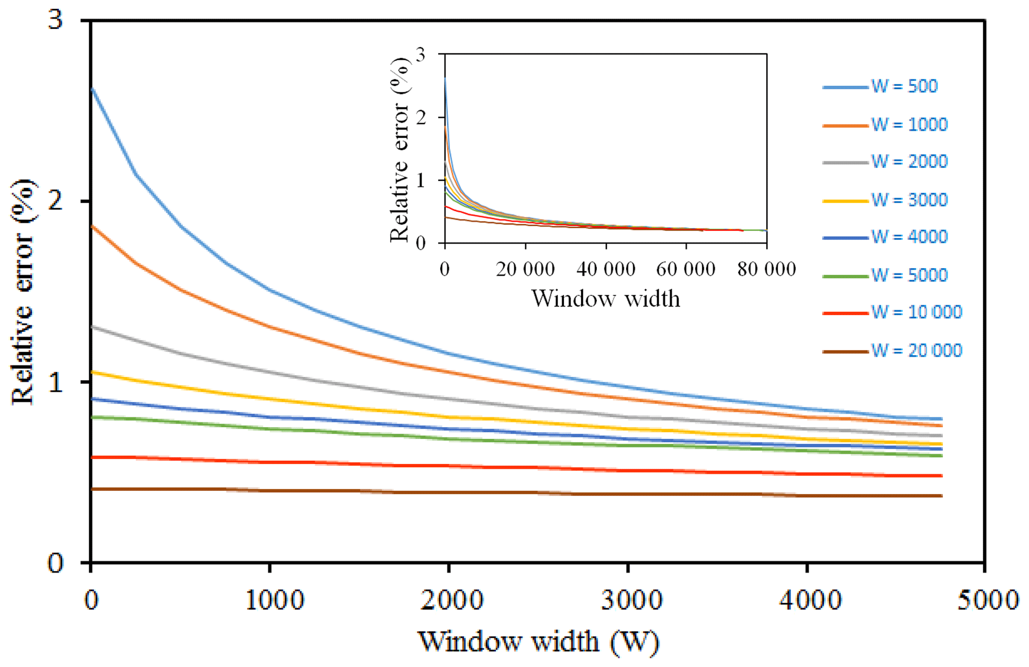
Figure 4 Relative error as a function of the given initial window width. For example, the cyan line corresponds to an initial window width of W = 500, for which the calculated relative error in entropy is 2.7 %.

The threshold magnitude and width of the window for the windowing process have been set to M₀=2.2 and W = 3000, respectively; this reduced the size of the catalogue to 84 593 events. Finally, the third step is to get entropy H. The evolution of entropy with time from the windowing process is shown in Fig. 5. Sudden changes in entropy are evident and correspond to the times of the largest earthquakes. Levels of change in the absolute values of entropy increase with increasing earthquake magnitude. The entropy change for the Tocopilla earthquake reached H = 0.35, while for the Calama 2010 and 2011 earthquakes it barely exceeded H = 0.25. For the Iquique earthquake and its large foreshock and aftershock, the entropy value reached H = 0.45.

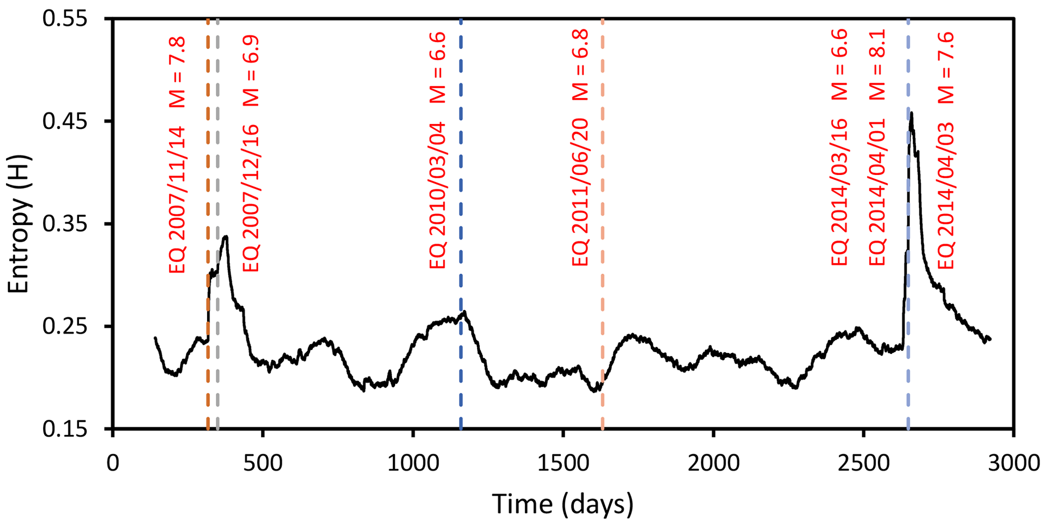
Figure 5 Time series of Shannon entropy, H, with the occurrence times of M_w > 6.5 earthquakes shown by dashed lines (note that the large foreshock, mainshock and large aftershock of the Iquique earthquake occurred close together in time; as such, only a single dashed line is shown). Sudden changes in entropy are clearly identifiable and coincident with large earthquakes.

Chilean seismicity is not only shallow seismicity; in fact, deep abundant earthquakes occur correspondingly to a subduction region; then, we also investigated entropy variation as a function of earthquake type, as defined by depth (Figs. 1c and 6), as follows: zone A, intraplate earthquakes characterized by shallow depth (0–80 km) and a tectonic origin; zone B, interplate earthquakes characterized by intermediate depth (80–160 km) and related to the contact between the two plates; and zone C, slab earthquakes that occur at large depths (> 160 km) in the slab of the underlying plate.

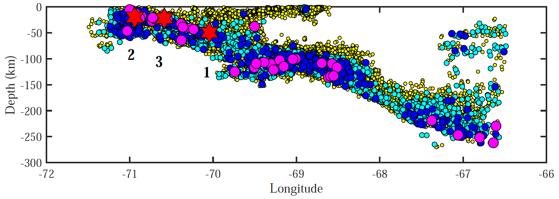
Figure 6 Earthquake depth versus longitude for earthquakes with magnitudes of > 2.0. Circle colours denote event magnitudes: yellow is 2.0–3.9, cyan is 4.0–4.9, blue is 5.0–5.9 and magenta is 6.0–6.9. Red stars denote earthquakes with magnitudes of > 7.0, including the (1) 2007 M_w 7.8 Tocopilla earthquake, (2) 2014 M_w 8.1 Iquique earthquake and (3) 2014 M_w 7.6 aftershock of the Iquique earthquake.

Figure 7 Epicentrally represented earthquake activity and non-cumulative and cumulative Gutenberg–Richter relationships in zones A–C for earthquakes with magnitudes of > 3.0. (a, d) Zone A (0–80 km), (b, e) zone B (80–160 km) and (c, f) zone C (> 160 km). Symbol colours denote earthquake magnitude: yellow circles are 3.0–3.9, cyan circles are 4.0–4.9, blue circles are 5.0–5.9, green triangles are 6.0–6.9 and red stars are > 7.0. Based on the maximum curvature (MAXC) technique (Wiemer and Wyss, 2000), M₀ = 2.2 in zones A and B and 3.2 in zone C.

The analysis of threshold magnitudes for zones A, B and C as well as the calculation of window W were as described above for the previous calculation of H (see Fig. 7 for epicentral maps of the three zones and the computation of M₀ in each). Figure 8 shows the time series of entropy for each of the three zones. In zone A, sudden changes in entropy were coincident with the Tocopilla and Iquique earthquakes. Zones B and C show low-amplitude sawtooth fluctuations in entropy (maximum ΔH of ≤ 0.09 vs. ΔH≈0.5 in zone A). The entropy variations in zones B and C are negligible compared with those in zone A.

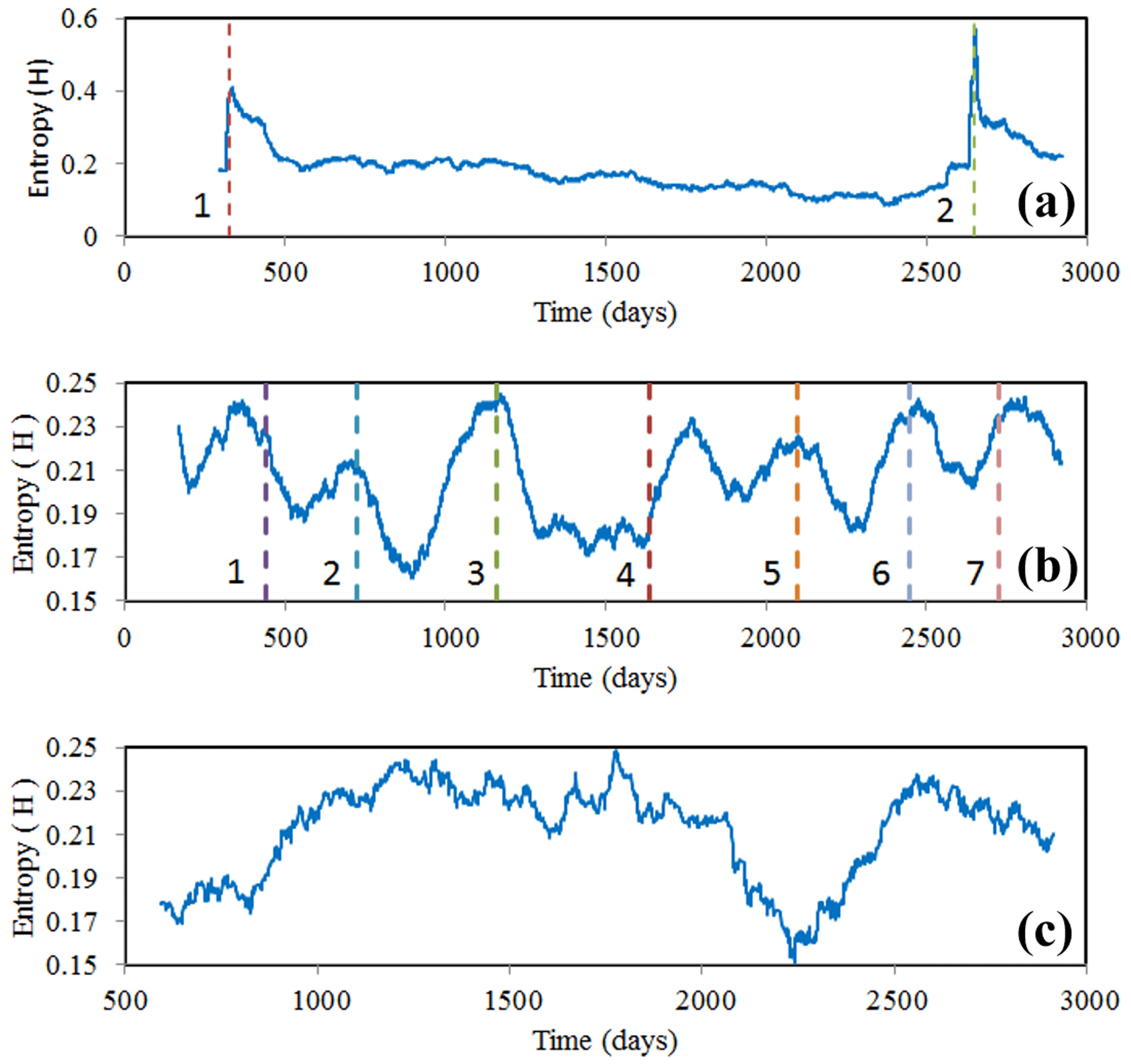
Figure 8 Time series of Shannon entropy, H, within different depth intervals. (a) Zone A (earthquakes with depths of 0–80 km), (b) zone B (80–160 km) and (c) zone C (> 160 km). The relative change in entropy in zone A is ∼ 0.5 units compared with 0.09 units in zones B and C. Lines 1 and 2 in (a) correspond to the 2007 M_w 7.8 Tocopilla earthquake and M_w 8.1 Iquique earthquake, respectively; lines 1 to 7 in (b) correspond to the M_w 6.5 March 2008 earthquake, clusters of earthquakes with magnitudes ranging from 5.8 to 6.0 from December 2008 to March 2009, the 2010 M_w 6.6 Calama earthquake, the 2011 M_w 6.8 Calama earthquake, the 2012 M_w 5.9 earthquake, clusters of earthquakes with magnitudes ranging from 5.9 to 6.2 from July 2013 to January 2014​​​​​​​ and the two 2014 M_w 6.2 earthquakes.

In zone B (Fig. 8), the 2010 and 2011 Calama earthquakes (M_w 6.6 and M_w 6.8 events on days 1158 and 1631, corresponding to 4 April 2010 and 20 June 2011, respectively) are clearly identifiable by increases in entropy. Other peaks before and after these earthquakes are coincident with either smaller earthquakes or clusters of smaller earthquakes (M_w 5.5–6.5), including a M_w 6.5 event on 24 March 2008 (day 448); a group of earthquakes between 4 December 2008 and 27 March 2009 (days 703–816, magnitudes of 5.8–6.0); a M_w 5.9 earthquake on 8 August 2012 (day 2107); a cluster of earthquakes between 10 July 2013 and 7 January 2014 (days 2382–2563, magnitudes of 5.9–6.2); and two earthquakes on 31 March and 23 August 2014, both with magnitudes of 6.2 (days 2646 and 2791, respectively).

A visual analysis of Fig. 8 seems to indicate that there is a periodic behaviour in the temporal signal of entropy; although this behaviour seems evident in zone B, it is not so evident in zones A and C. Zone A is associated with a stress loading rate usually not uniform in time because, as is well known, the strength of the crust is not constant; then, change in entropy was only appreciated when the two great earthquakes occurred. On the other hand, zone C, where the most complex physical phenomena occur due to the rheological state of the materials, seems to exhibit a half period in the entropic signal, but this must be confirmed in further studies with up-to-date data. The apparent periodicity in zone B suggests carrying out a Fourier analysis of the entropic signal. The entropic signal is not uniformly sampled in the time domain; for this reason, it was averaged to the 10th part of the day, and, subsequently, an interpolation was made for points with no sample. Thus, the resulting entropic signal was uniformly sampled, and a fast Fourier transform was feasible.

The Fourier transform of the entropic signal (Fig. 9) revealed that the peaks of the predominant amplitude have frequencies of 0.00048 and 0.00119 d⁻¹, corresponding to periods of ∼ 2100 and 840 d, respectively. The 840 d period approximately reproduces the sequence of M > 5.5 earthquakes. For instance, 840 d after the Tocopilla earthquake (14 November 2007) was 3 March 2010, which is 1 d before the Calama 2010 earthquake. However, given the relatively short period covered by the data (8 years), this Fourier analysis is necessarily preliminary. Further studies with observation periods from 2015 until the present are needed to confirm these results.

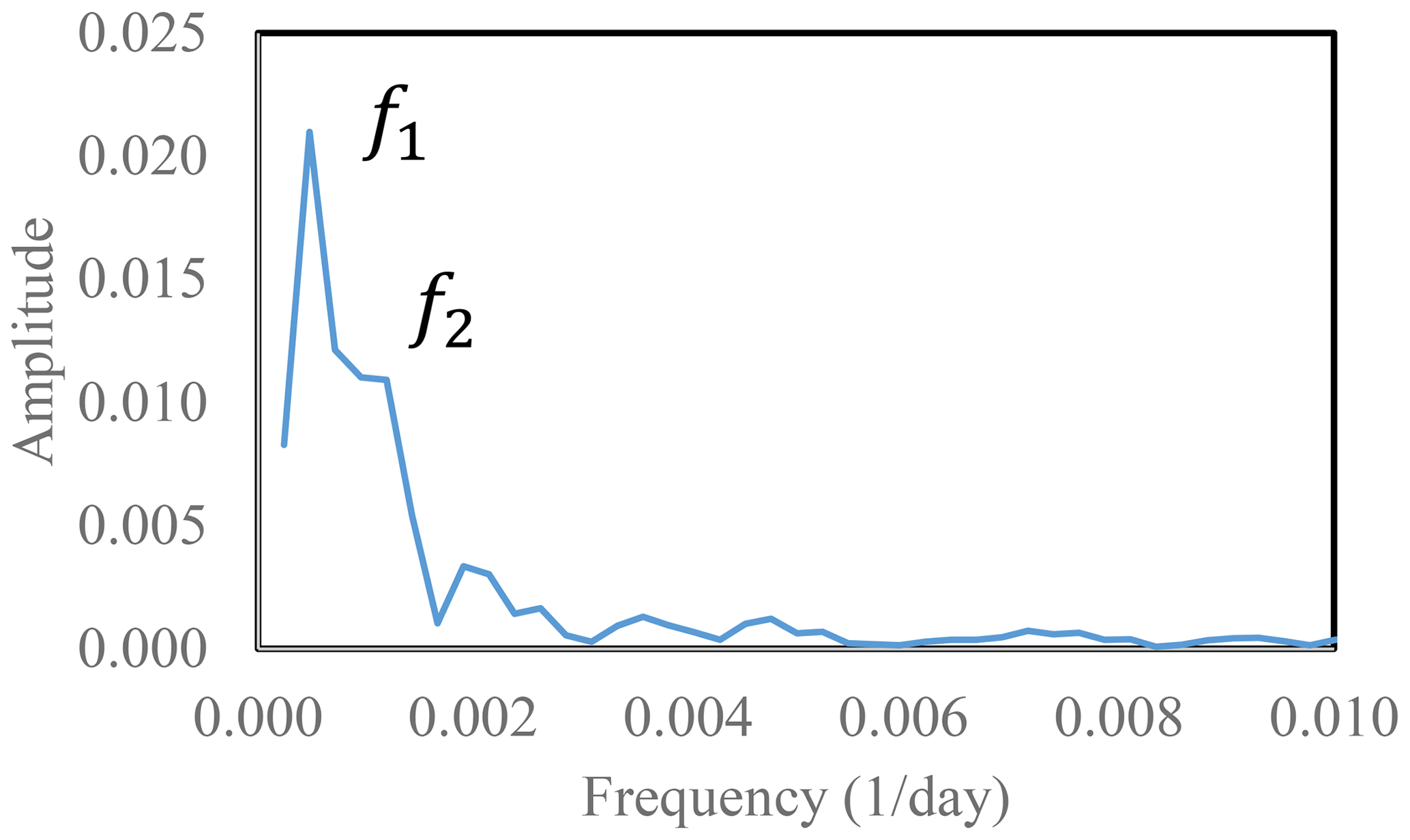
Figure 9 Spectrum for the entropic signal of zone B (80–160 km). The two peak amplitudes have frequencies of f₁=0.00048 d⁻¹ and f₂=0.00119 d⁻¹, corresponding to periods of ∼ 2100 and 840 d, respectively.

5 Discussion and conclusions

It is widely accepted that the seismic cycle (or seismic system) comprises six main stages (Fig. 10) (Derode et al., 2021; Akopian and Kocharian, 2014). The stages are (1) over decades or years, small and medium asperities break continuously, resulting in a uniform rate of seismicity. (2) Asperities become locked, resulting in stress accumulation and decreasing seismic activity. (3) Weeks or days before a mainshock, important asperities progressively break along some sections (i.e. the foreshock stage). (4) Over a scale of hours, accumulated stresses overcome friction and blockages in the main asperities, causing the largest-magnitude earthquake of the cycle. (5) Stress relaxation occurs after the mainshock and is characterized by numerous aftershocks of smaller magnitude over several weeks or months; this ceases when new asperities become locked. (6) Finally, the system returns to the initial long-term state.

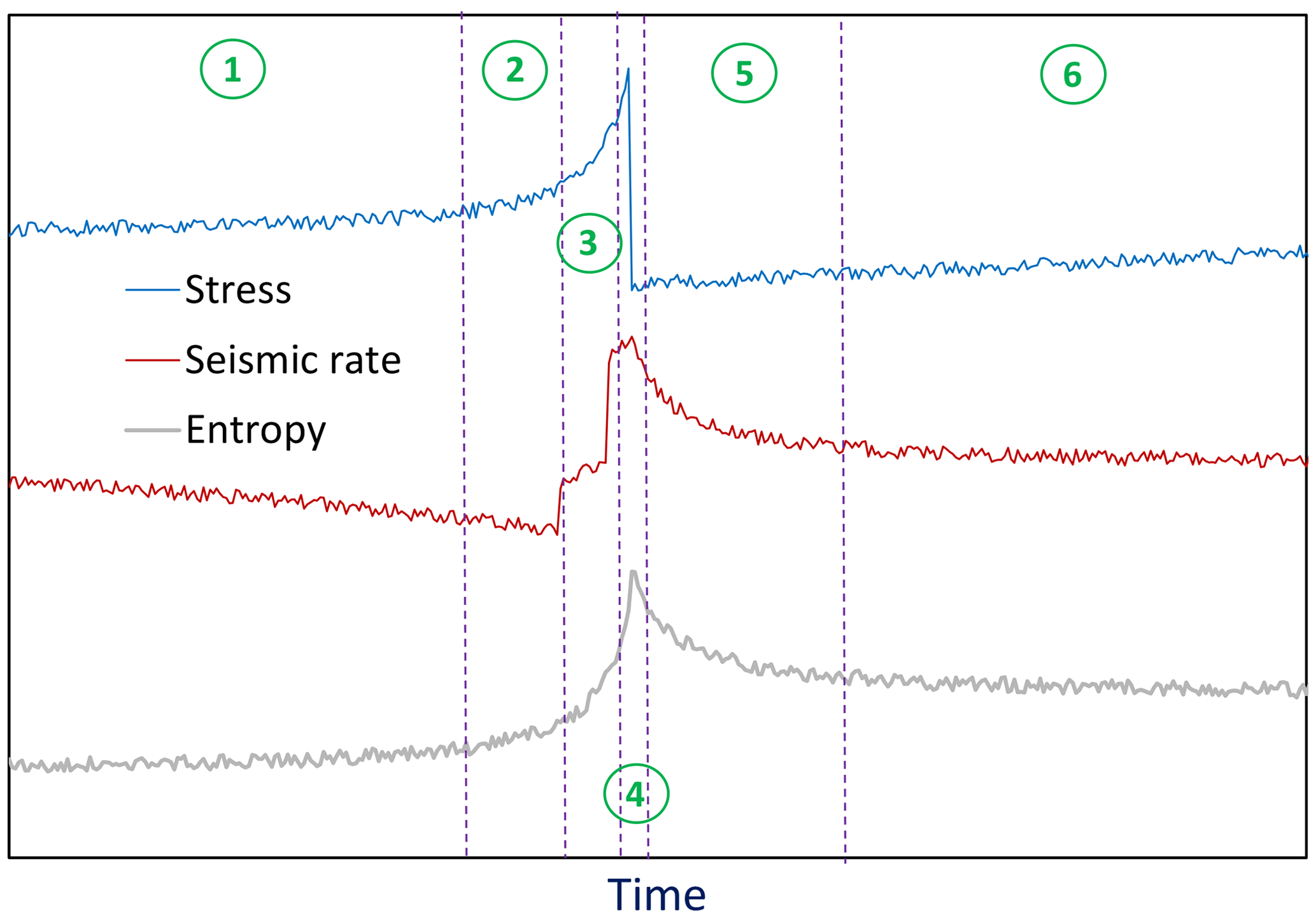
Figure 10 Seismic cycle from a mechanical perspective (i.e. stresses and seismic rate, which are shown in blue and red, respectively) and from a thermodynamic perspective (i.e. entropy, H, which is shown in grey). (1) Stage 1, the interseismic period, is characterized by approximately constant stress, seismic rate and H. (2) Stage 2, the accumulation period, is characterized by modest increases in stress and H but a modest decrease in seismic rate. (3) Stage 3, the foreshock period, is characterized by increasing stress, seismic rate and H. (4) Stage 4, the coseismic period, is characterized by an abrupt decrease in stress but increases in the seismic rate and H. (5) Stage 5, the postseismic and aftershock period, is characterized by decreasing stress (i.e. relaxation), seismic rate and H (towards the initial value). (6) Stage 6 is during which the seismic cycle starts again.

In this paper, we have visualized that this mechanical description of the seismic cycle has an energetic analogy in terms of statistical physics and the second law of thermodynamics. As argued in detail by De Santis et al. (2019), an earthquake can be considered a phase transition, where continuous reorganization of stresses and forces reflects an evolution from equilibrium to non-equilibrium states. Therefore, entropy, which measures the number of accessible states for the present conditions of the systems, can be used as an indicator of the evolution of the system (e.g. Telesca et al., 2004; Vogel et al., 2020). Stages 1–3 correspond to increasing stresses and the accumulation of seismic energy. During this interseismic period, the magnitudes of earthquakes are relatively uniform (or “ordered”), and entropy is relatively low. When a large earthquake occurs (stage 4), the rupture process triggers earthquakes with magnitudes of all sizes in a chaotic way, evolving to new conditions reaching a wider range of microstates in a disordered way, and the entropy increases. Finally, during the postseismic state (stages 5 and 6), the system progressively recovers conditions similar to the initial ones.

Increasing entropy, H, from a thermodynamic perspective, is associated with an irreversible transition from one state to another on both small (Scholz, 1968) and large (e.g. Parsons et al., 2008) scales. Using a high-quality catalogue of seismicity in northern Chile, made possible owing to the IPOC network, we confirmed a strong temporal correlation between entropy and the occurrence of earthquakes. Using the entropy value, we could identify all earthquakes with magnitudes of > 6.5 in the catalogue (i.e. seven events from 2007 to 2014, with magnitudes ranging from 6.6 to 8.1).

However, it is important to note that changes in entropy are detected by analysing the entire catalogue; that is, to detect a change in entropy associated with any event, data from both before and after the event must be analysed. At present, this limits the use of this method for seismic prediction. Further research is needed to determine a robust approach for predicting how a time series will continue without prior knowledge, that is, to determine threshold entropy values and trends that can be used to predict a significant event in the immediate future. To achieve this, an absolute scale of entropy will be necessary. Earthquakes in zone A (0–80 km depth) tend to be tectonic in origin and have higher magnitudes than those in zones B and C (i.e. intermediate and deep earthquakes); as such, they are of most concern from a risk management perspective. Our results show that the entropy changes associated with such events are much stronger when only data from this depth interval are considered; variations are of the order of 100 in zones B and C but several 10ths in zone A.