An assessment of short–medium-term interventions using CAESAR-Lisflood in a post-earthquake mountainous area

The 2008 Wenchuan earthquake triggered rapid local geomorphic changes, shifting abundant material through exogenic processes and generating vast amounts of loose material. The substantial material movement increased the geohazard (flash floods, landslides and debris flows) risks induced by extreme precipitation in the area. Intervention measures such as check dams, levees and vegetated slopes have been constructed in specific locations to reduce sediment transport and thereby mitigate the impact of ensuing geohazards.

This study assessed the short–medium-term effects of interventions, including multiple control measures, in a post-earthquake mountainous region. Taking the Xingping valley as an example, we used CAESAR-Lisflood, a two-dimensional landscape evolution model, to simulate three scenarios, unprotected landscape, present protected landscape and enhanced protected landscape, between 2011 and 2013. We defined two indices to assess the intervention effects of the three scenarios by comparing the geomorphic changes and sediment yields.

The results show that the mitigation measures are effective, especially the geotechnical engineering efforts in combination with ecological engineering in the upstream area. The spatial patterns of erosion and deposition change considerably due to the intervention measures. Additionally, the effectiveness of each intervention scenario shows a gradual decline over time, mainly due to the reduction in the reservoir storage capacity. The enhanced scenario performs better than the present one, with a more gradual downward trend of effectiveness. The simulation results evaluated the ability and effectiveness of comprehensive control measures and will support optimal mitigation strategies.

1 Introduction

Strong earthquakes can trigger co-seismic landslides and discontinuous rock masses in mountainous areas, which can increase erosion (Huang, 2009). Consequently, the movement of material through co-seismic landslides and attendant mass failures modifies mountain landscapes through various surface processes for days, years and millennia (Fan et al., 2020). The 2008 Wenchuan earthquake with a surface-wave magnitude (M_s i.e. the logarithm of the maximum amplitude of the ground motion of the surface waves with a wave period of 20 s) of 8.0 has influenced towns and other infrastructure in the affected area. Many studies have mapped the landslides triggered by this devastating earthquake. Gorum et al. (2011) performed an extensive landslide interpretation using a large set of high-resolution optical images and mapped nearly 60 000 individual landslides, impacting an area of 600 m² or more. Xu et al. (2014) delineated 197 481 landslides represented by polygons, centroid points and top points compiled from visual image interpretation. To estimate the impact of loose material on subsequent sediment transport caused by landslides, some researchers attempted to calculate the volume of deposited material based on field surveys and assumptions. For example, Huang and Fan (2013) estimated that 400×10⁶ m³ of material was deposited in heavily affected area by assuming that the material was deposited on steep slopes with angles greater than 30^∘ and a catchment area of more than 0.1 km². An approximate 2793×10⁶ m³ of debris was calculated by Chen et al. (2009) using different deposition depth settings in different buffer zones of the Longmenshan central fault. In summary, a tremendous amount of loose material accumulated in gullies and on hillslopes in earthquake-affected catchments, which became available for erosion events for years to come.

To mitigate the above-mentioned hazards and protect the landscape, including downstream settlements, structural mitigation measures have been developed in the affected area, depending on the different site-specific conditions, in addition to technical and economic feasibilities. For example, slope protection with vegetation was conducted to stabilise source material on hillslopes (Cui and Lin, 2013; Forbes and Broadhead, 2013; Stokes et al., 2014). Check dams were also widely used to intercept upriver sediment (Yang et al., 2021; Marchi et al., 2019). Lateral walls and levees, which are longitudinal structures (Marchi et al., 2019), are used to protect settlements near main channels with relatively high levels of sediment discharge.

Although comprehensive control measures have been taken in potentially dangerous sites, improvement of mitigation performance in the Wenchuan earthquake-stricken area is still ongoing. The seasonal and periodic occurrence of massive sediment transport often particularly affects the mountainous area. This might be caused by intense precipitation and the failure of mitigation measures due to rough terrain, vague information about source storage and sometimes relatively low-cost mitigation measures (Yu et al., 2010; Cui et al., 2013). Therefore, understanding and quantifying the effectiveness of intervention measures is crucial for mitigation strategies. Many studies have focused on establishing post-evaluation effectiveness index systems that are not supported by sufficient practices (Zhang and Liang, 2005; Wang et al., 2015). Some researchers compared the changes before and after intervention measures by recording long-term on-site measurements, which require a great deal of time, energy and financing (Zhou et al., 2012; Chen et al., 2013). More recently, studies have compared disaster characteristics before and after mitigation actions through quick calculations using numerical simulations (Cong et al., 2019; He et al., 2022). Nevertheless, these studies ignore the lasting effects of earthquakes on geomorphic changes (longer than the duration of a single event). Therefore, the short–mediu- term (from the duration of a single event to decades after) geomorphic changes obtained from simulations provide more details to interpret engineering measures in notable locations, even in locations inaccessible to humans.

CAESAR-Lisflood (C-L), a two-dimensional hydrodynamic surface landscape evolution model based on the cellular automata (CA) framework, has powerful spatial modelling and computing capabilities (Coulthard et al., 2002, 2013; Van De Wiel et al., 2007; Bates et al., 2010). C-L is used widely in rehabilitation planning and soil erosion predictions in post-mining landscapes (Saynor et al., 2019; Hancock et al., 2017; Lowry et al., 2019; Thomson and Chandler, 2019; Slingerland et al., 2019) as well as studies in channel evolution and sedimentary budget planning for dam settings (Poeppl et al., 2019; Gioia and Schiattarella, 2020; Ramirez et al., 2020, 2022). The applications presented demonstrate the efficiency of C-L model to simulate the surface material migration and landscape evolution after anthropogenic and natural disturbances, which indicates the potential to simulate the complexity of surface processes integrated with different interventions. In addition, many studies applied C-L to investigate the landscape evolution after the Wenchuan earthquake (Li et al., 2020; Xie et al., 2022a, b, 2018). The configuration of the model can be referenced to the study of intervention scenarios in the same post-earthquake region.

In this study, we investigated the impact of different interventions on sediment dynamics and geomorphic changes in an earthquake-stricken valley. Hourly rainfall data over 3 years were generated by daily downscaling to capture extreme events. We then simulated and compared the geomorphic changes and sediment yield in three scenarios that varied in their mitigation compositions and intensities in the catchment. The objectives were (1) to assess the effectiveness of a set of mitigation measures to reduce sediment transport, (2) to analyse the role of each measure on geomorphic changes and (3) to determine the influence of vegetation on catchment erosion.

2 Study area

2.1 Regional characteristics

The study area was the Xingping valley, the left branch of the Shikan River (a tributary of the Fu River) in north-eastern Sichuan Province (Fig. 1). Nearly 200 settlements are scattered in the study catchment. The catchment has a total drainage area of approximately 14 km² and a rugged topography, with an elevation ranging from 800 to 3036 m, which is characterised by a high longitudinal gradient (∼120 ‰) and distributed more than 10 small V-shaped branch gullies. The region has a humid temperate climate with a mean annual temperature of 14.7 ^∘C. The mean annual precipitation is 807.6 mm, with more than 80 % concentrated between May and September. The steep terrain and heavy rainfall are combined to control the nature of the ephemeral streams in this area.

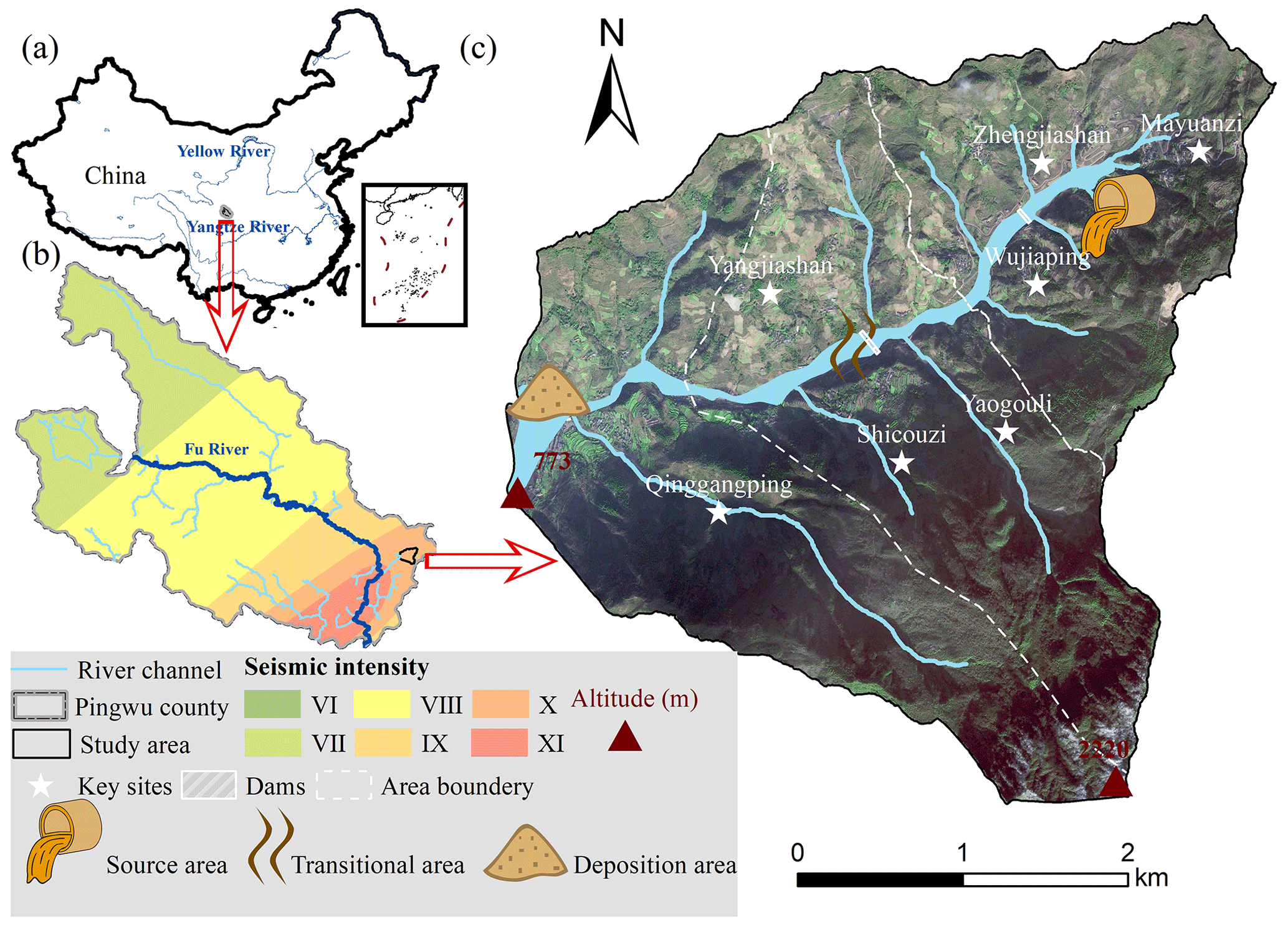
Figure 1 An overview of the study area. (a) The location of the study area, (b) a seismic intensity map of the Wenchuan earthquake within Pingwu County and (c) a schematic image of the study area.

The basement rocks in the study area are mainly metamorphic sandstone, sandy slate, crystalline limestone and phyllite of the Triassic Xikang Group (T_3xk) and Silurian Maoxian Group (S_mx), which are easily eroded by in situ weathering processes after disturbances caused by strong earthquakes. Consequently, the Wenchuan earthquake, with a modified Mercalli intensity scale of X, made this area one of the most severely affected regions (Wang et al., 2014) and produced 10⁶ m³ of loose material by triggering landslides and subsequent erosion in Mayuanzi, Zhengjiashan and Wujiaping (Fig. 1) (Guo et al., 2018).

2.2 Historical hazards and intervention measures

Six debris flow flash-flood disaster chain groups have been found in the Xingping valley over the decade after the earthquake. Based on the published work of SKLGP (State Key Laboratory of Geohazard Prevention and Geoenvironment Protection), the geological survey of local government and our biannual field surveys since 2012, we catalogued the time of occurrence, total rainfall and corresponding disaster details of each event (Table S1 in the Supplement). A massive amount of sediment was transported soon after the devastating earthquake in 2008 and 2009. Extensive loose materials were then delivered and deposited in the channel triggered by the extreme rainfall events in 2013 and 2018. Considering the transport processes of landslide material, we divided the study area into three subregions: the source area, the transitional area and the deposition area (Fig. 1). The dashed white lines in Fig. 1c indicate that the loose material can be easily transported from the source area to the deposition area through the transitional zone.

An engineering control project was constructed in the study valley to intercept the upriver material in October 2010. The project included two check dams, with one located in the upper source area and the other located in the transitional zone (Feng et al., 2017) (Fig. 1c). The upper dam has a storage capacity of 5.78×10⁴ m³ and a height of 10.0 m. The dam at transitional area has a storage capacity of 7.2×10⁴ m³ and a height of 9.0 m. The first dredging work was subsequently performed in 2013 due to gradual filling of the reservoirs. Nearly 3 years later, the storage capacity behind the upper dam remained at 50 % in 2016, while the transitional area dam could no longer retain sediment.

3 Materials and methods

In this study, we examined the intervention effectiveness through the morphological response and sediment yield in the Xingping valley using the C-L simulations. The research entailed four main steps: (1) setting three scenarios with different intervention measures, (2) pre-processing the model input data, (3) calibrating the hydrological component and (4) simulating geomorphic changes and analysing the intervention effectiveness during 2011–2013.

3.1 Scenario settings

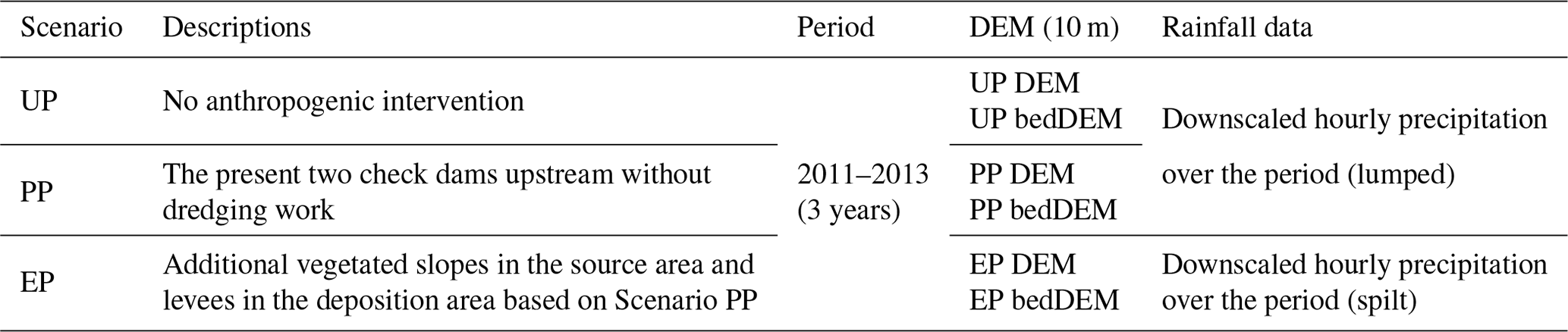
The abundant material mobilised by landslides should be controlled in order to reduce the sediment transport. Therefore, we designed three scenarios by integrating geotechnical engineering with ecological engineering to assess the effectiveness of intervention measures. In Scenario UP, unprotected landscape means the sediment is transported without anthropogenic intervention. In Scenario PP, present protected landscape means that only the present two check dams trapped sediment during 2011–2013 without dredging work over this period (see Sect. 2.2). In Scenario EP, enhanced protected landscape represents the addition of slope protection with vegetation in the source area and levees in the deposition area, in addition to the two check dams in Scenario PP.

Figure 1c shows the locations of the existing two check dams in both Scenario PP and Scenario EP. We determined the placements of additional measures in Scenario EP according to a field survey, which demonstrated that the continuous supply of sediment is mainly from the source area. Therefore, vegetated slopes were designed in the upstream area to prevent erosion by stabilising the topsoil and enhancing the soil's infiltration capacity via roots (Lan et al., 2020).

Considering the damage caused by flash floods to the residential area downstream, the levees (see Fig. S1 in the Supplement and Sect. 3.2.2), i.e. artificial barriers, were placed to protect agricultural land and buildings by preventing water and sediment from overflowing and flooding the surrounding areas. Table 1 shows the scenario descriptions, initial model conditions and input rainfall. The details about the model and input data are introduced in Sect. 3.2.

Table 1 Scenario settings.

3.2 CAESAR-Lisflood

The C-L integrated the Lisflood-FP 2D hydrodynamic flow model (Bates et al., 2010) with the CAESAR landscape evolution model (LEM) (Coulthard et al., 2002; Van De Wiel et al., 2007), which is described in detail by Coulthard et al. (2013). The catchment mode of C-L was applied in this study, in which the surface digital elevation model (DEM), the bedrock DEM (bedDEM), the grain size distribution and a rainfall time series are required to simulate the geomorphic changes and sediment transport. There are four primary modules within C-L that are implemented as follows:

1. a hydrological module generates surface runoff from rainfall input using an adaptation of TOPMODEL (topography-based hydrological model) (Beven and Kirkby, 1979),

2. a hydrodynamic flow routing module based on the Lisflood-FP method (Bates et al., 2010) calculates the flow depths and velocities,

3. an erosion and deposition module uses hydrodynamic results to drive fluvial erosion by either the Einstein (1950) or the Wilcock and Crowe (2003) equations, which are applied to each sediment fraction over nine different grain sizes,

4. and a slope module of material movement from the hillslope into the fluvial system, taking into account both mass movement when a critical slope threshold is exceeded and soil creep processes, where sediment flux is linearly proportional to surface slope.

The C-L model updates variable values stored in square grid cells at intervals such as DEM, grain size and proportion data, water depth, and velocity. For the three scenarios, the initial conditions, such as the DEM, bedDEM, rainfall data and the m values, were pre-processed as follows.

3.2.1 The surface and bedrock digital elevation models

To clearly describe the control process, especially the two dams and levees in the catchment, we unified grid cell scales to 10 m for all input data of the C-L. The GlobalDEM product with a 10 m×10 m resolution and 5 m (absolute) vertical accuracy was used to form three types of initial DEMs (UP DEM, PP DEM and EP DEM). Before rebuilding the initial DEMs, we filled the sinks of the original GlobalDEM based on the Environmental Systems Research Institute's (ESRI's) ArcMap (ArcGIS, 10.8) to eliminate the “walls” and the “depressions” in the cells and thus avoided intense erosion or deposition in the early run time. Then, the modified DEM was used as the surface DEM in Scenario UP (UP DEM) without any mitigation measures. According to the engineering control project described in Sect. 3.2.2, the surface DEM of Scenario PP (PP DEM) included the dams by raising the grid cell elevations by 10 m for the dam in the source area and 9 m for the dam in the transitional zone. Similarly, the surface DEM in Scenario EP (EP DEM) included the dams in the PP DEM. In addition, two levees were produced by raising the grid cell elevation by 2 m at selected locations. For Scenario EP, the placement and setting of the vegetation protection are introduced in Sect. 3.2.2.

The spatial heterogeneity in the source material (Fig. 1c) results in differences in the erodible thickness, which equals the difference between the surface DEM and the bedDEM. We divided the study area into five regions according to the erodible thickness (Fig. S1) by checking the relative elevation of the foundations of buildings, the exposed bedrock and the deposition depth of landslides with respect to ground level. The average thicknesses in upstream low- and high-elevation areas were set to 10 and 3 m, respectively, and the thickness of the erodible layer in the downstream area was set to 3 m. For the river channel and outlet, where there would be a large amount of deposition, the thickness of erodible sediment was set to 5 and 4 m, respectively. As the dams in Scenario PP and the levees in Scenario EP were non-erodible concrete, we set the erodible thickness of these features to 0 m. Eventually, the DEM data were formatted to ASCII raster data as required by C-L. The additional levees and vegetated slopes in Scenario EP and the pre-processes of the DEMs and bedDEMs are shown in Fig. S1.

3.2.2 Vegetation settings

Another parameter required in each scenario simulation was the m value of the hydrological model (TOPMODEL) within C-L, which controls an exponential decline in transmissivity with depth (Beven, 1995, 1997) and influences the peak and duration of the hydrograph in response to rainfall. The m value effectively imitates the effect of vegetation, which controls the fluctuation of the soil moisture deficit and thus influences the peak of the modelled flood hydrograph (Coulthard et al., 2002). The m value is usually determined by the land cover (e.g. 0.02 for forests and 0.005 for grasslands) (Coulthard and Van De Wiel, 2017). In our study, we set the m value to 0.008 in the catchment (14 km²) in Scenarios UP and PP, which resembles the m value of farmland with lower vegetation cover studied by Xie et al. (2018) and Li et al. (2018). As mentioned earlier, the upstream low-elevation area protected by vegetation in the EP scenario was assigned a higher m value of 0.02. This m value was calibrated by the more extensive catchment containing our study area in the flood event of 2013 (Xie et al., 2018).

3.2.3 The rainfall data

In this research, we compared three scenarios by matching precipitation data between 2011 and 2013, as mentioned in Sect. 3.1. The source data of precipitation in 2011–2013 (Fig. 2a) were obtained from the Resource and Environment Science and Data Center​​​​​​​ (https://www.resdc.cn/Default.aspx, last access: 30 March 2023) with daily temporal resolution. The intensity and frequency of extreme rainfall events affects patterns of erosion and deposition (Coulthard et al., 2012b; Coulthard and Skinner, 2016). Therefore, we used the stochastic downscaling method to generate hourly data to better capture the hydrological events introduced by Li et al. (2020) and Lee and Jeong (2014). The referenced hourly precipitation was observed from the pluviometer located 20 km from the study area in 2016 (Fig. 2b), with an annual total precipitation of 684 mm. The observed rainfall in 2016 was characterised by (1) hourly precipitation between 1.1 and 35.4 mm and (2) maximum and average durations of rainfall events of 24 and 2.8 h, respectively. The main processes of the downscaling method are as follows:

• extracting the hourly rainfall of specific days in 2016 closest to the daily rainfall in 2011–2013 through the threshold setting and producing the genetic operators using the extracted hourly rainfall dataset;

• mixing the genetic operators by an algorithm (Goldberg, 1989) composed of reproduction, crossover and mutation and repeating these processes until the distance between the sum of hourly rainfall and the actual daily rainfall was less than the set threshold;

• normalising the hourly precipitation to keep the daily rainfall value unchanged.

Figure 2c shows the downscaled rainfall series between 2011 and 2013. The downscaled hourly rainfall better captured the hydrological events at an hourly scale compared to the hourly mean rain (5.27 mm) on the day with extreme rainfall (126.5 mm), which was far from the actual situation. Corresponding to the m value settings, the input of generated hourly precipitation was lumped catchment-wide in Scenario UP and Scenario PP and divided into two separate but identical rainfall events in Scenario EP.

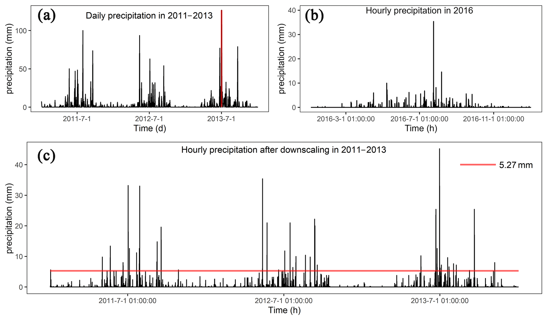
Figure 2 (a) Daily precipitation in 2011–2013 (the red vertical line indicates the maximum daily precipitation of 126.5 mm), (b) hourly precipitation in 2016 and (c) downscaled hourly precipitation in 2011–2013 (the horizontal red line indicates the hourly mean precipitation of 5.27 mm on the day with the maximum precipitation marked in panel a).

3.2.4 Other parameters

As introduced by Skinner et al. (2018), the C-L model is sensitive to a set of input data for a catchment with a grid cell size of 10 m, such as the sediment transport formula, slope failure threshold and grain size set. The grain size distribution of sediment was derived from sampling at 14 representative locations in the same study basin by Xie et al. (2018). Given the grain size distribution in this study, the Wilcock and Crowe formula was selected as the sediment transport rule, which was developed from flume experiments using five different sand–gravel mixtures with grain sizes ranging between 0.5 and 64 mm (Wilcock and Crowe, 2003). Considering the steep slopes on either side of deep gullies, a higher slope failure threshold was determined to replicate the geomorphic changes between 2011 and 2013. Additionally, we found that the probability of shallow landslides increased with increasing slope gradient from 20 to 50^∘ between 2011 and 2013 (Li et al., 2018). The slope angle was derived from the DEM with a 30 m spatial resolution, which caused a lower slope angle than that with a 10 m resolution. As such, we set the slope angle to 60^∘, which is lower than the 65^∘ used in a scenario without landslides (Xie et al., 2022a) and higher than 50^∘. Some parameters were determined by repeated experiments, such as the minimum Q value, and the other input values were set to default values recommended by the developers (such as the maximum erosion limit in the erosion/deposition module and the vegetation critical shear stress) in https://sourceforge.net/p/caesar-lisflood/wiki/Home/ (last access: 30 March 2023). Table S2 presents the model parameters of C-L used in this study.

3.2.5 Model calibration

Because the basin was ungauged before 2015, we replicated the flash flood event in July 2018 using C-L simulations to calibrate the hydrological components. Based on Scenario PP (with two check dams), we used the 2-week hourly precipitation of July 2018 as the input (Fig. S2a), which was recorded by a rain gauge located 2.5 km from the catchment (Fig. S2b). The simulation results (Fig. S2c and d) yielded an erosion map and a maximum water depth map in Scenario PP on 15 July 2018. We selected three locations to compare the deposition and inundation in the simulation results with satellite images and photos (Fig. S3). The simulated sediment thickness and water depth were close to those measured from the images, which indicated that the flash flood event was well replicated by the C-L using the input data.

3.3 Output analysis

The C-L model outputs of each scenario include hourly water and sediment discharge at the basin outlet and EleDiffs (the difference between modelled DEM at a specified time and initial DEM). We validated the model outputs by comparing the hourly discharge and EleDiffs reflecting the depth of sediment deposition or erosion (>0.1 m: deposition, $<-\mathrm{0.1}$ m: erosion) with field survey materials. The overall temporal and spatial geomorphic changes reflected by EleDiffs under three different scenarios were used to assess the geomorphic response to interventions. To explore the geomorphic response to various control measures, we focused on the notable sites where the check dams, levees and vegetated slopes were located and recorded the depth of accumulating sediment behind the two dams. To further explore the spatial heterogeneity we compared the volumes of deposition and erosion among the three divided regions, including the source area, the transitional area and the deposition area.

Based on the visual analysis and quantitative results, we defined two formulae to assess the effectiveness of the intervention. The conservation ability (Ca, Eq. 3) was calculated based on variables in the sediment balance system (Fig. 3). The sediment volume of deposited sediment (D_n) and input sediment from the upper connected region (I_n) are equal to that of the eroded material (E_n) and the output sediment to the next part (O_n) over the same period (Eqs. 1 and 2) in the system. A higher value of Ca in a specific region and scenario indicates a more effective control system.

$$\begin{array}{}\text{(1)}& {\displaystyle }{I}_n=\sum _{\mathrm{2}}^n{E}_{n-\mathrm{1}}-\sum _{\mathrm{2}}^n{D}_{n-\mathrm{1}},\text{(2)}& {\displaystyle }{I}_n+E_n=O_n+D_n,\text{(3)}& {\displaystyle }\text{Ca}={\displaystyle \frac{D_n}{I_n+E_n}},\end{array}$$

where n is the region number of the source area (=1), transitional area (=2) or deposition area (=3).

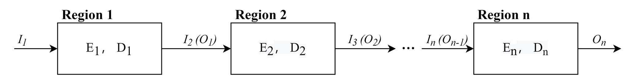
Figure 3 The sediment balance system in the study area (region n indicates the source area, transitional area or deposition area).

Additionally, we designed the relative efficiency (Re, Eq. 4) to depict the efficiency of intervention measures in Scenario PP and EP in sediment loss, with the comparison to Scenario UP.

$$\begin{array}{}\text{(4)}& {\text{Re}}_{\text{PP/EP},i}={\displaystyle \frac{Q_{\text{UP},i}-Q_{\text{PP/EP},i}}{Q_{\text{UP},i}}},\end{array}$$

where i is the sequence of the day, Q_UP is the daily sediment yield measured at the catchment outlet in Scenario UP, Q_PP/EP is the same data in Scenario PP or Scenario EP of day i, and Re_PP/EP is the daily relative effectiveness of control measures in Scenario PP or Scenario EP.

4 Results

4.1 Model verification

Figure 4 shows the input rainfall data and modelled discharge hydrograph between 2011 and 2013 (Fig. 4a). The comparisons of simulated mean discharge in April through July and the whole year with field survey materials in the two locations are also presented (Fig. 4b and c). Concerning the discharge hydrograph, the peak discharges (63.7, 54.9 and 50.3 m³ s⁻¹) correspond well with the peak rainfall intensities (31, 19.7 and 15 mm). The modelled water discharge from March–May in location A is slightly larger than the measured value reported by Feng et al. (2017). Additionally, an average annual discharge of 10.04 m³ s⁻¹ in location A is lower than that of 12.80 m³ s⁻¹ in the catchment outlet (location B), which has an area approximately 3 times the size of the study area.

Figure 4 The input and output of the hydrograph. (a) The input hourly precipitation and simulated discharge in 2011–2013 in Scenario PP, (b) the locations of the specified outlet points and (c) a comparison of the simulated average discharge to the recorded discharge.

Typical cross-sections are generated (Fig. 5) based on the replicated landform changes in Scenario PP. The first site is located on the upriver road, which is eroded to a depth of 5.7 m according to the simulation results, while the photo shows a depth of no less than 4.0 m without an apparent eroded base. Cross-section #2 and the site photo of the gully show that the eroded depth is approximately 1.0 m. Meanwhile, a clear sediment boundary is found in the building located in the deposition area (# 3), indicating a slightly lower deposition depth than the model predicted.

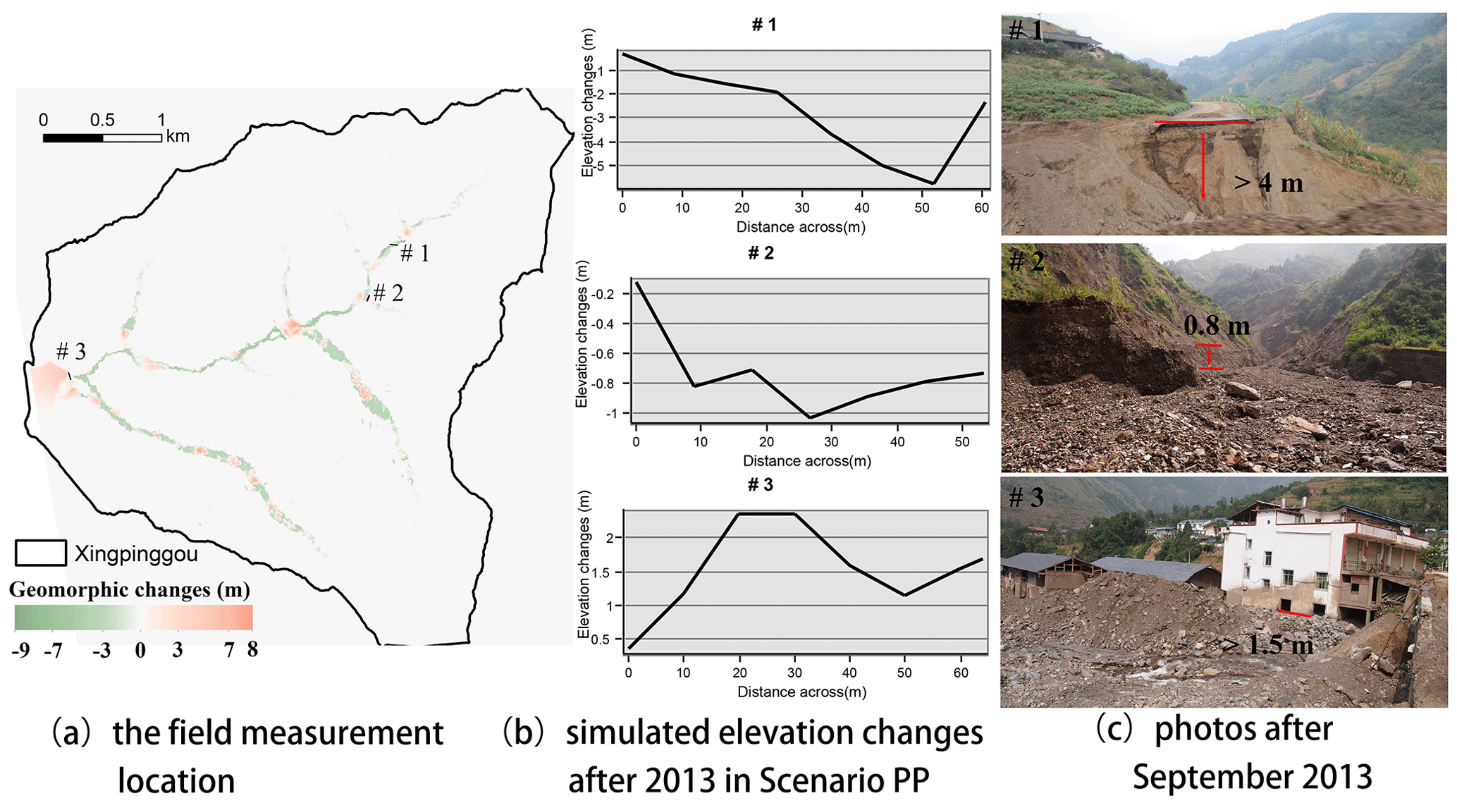
Figure 5 The comparison of cross-sections from the simulation results to the field measurements after 2013 in Scenario PP.

4.2 Overall geomorphic changes

Figure 6a compares the three annual landform changes in each scenario, which are classified into nine categories according to natural breaks for EleDiffs: extreme erosion ($<-\mathrm{7}$ m), heavy erosion (−7–3 m), moderate erosion (−3–1 m), light erosion (1–0.1 m), minor change (−0.1–0.1 m), light deposition (0.1–1 m), moderate deposition (1–3 m), heavy deposition (3–7 m) and extreme deposition (>7 m). A similar spatial pattern of erosion is observed in all three scenarios. More specifically, erosion mainly emerges in the main channel and the branch valleys, among which the left branches exhibit more pronounced erosion. In contrast, the deposition zone appears to vary in the three scenarios, especially in the area behind the two dams present in Scenarios PP and EP.

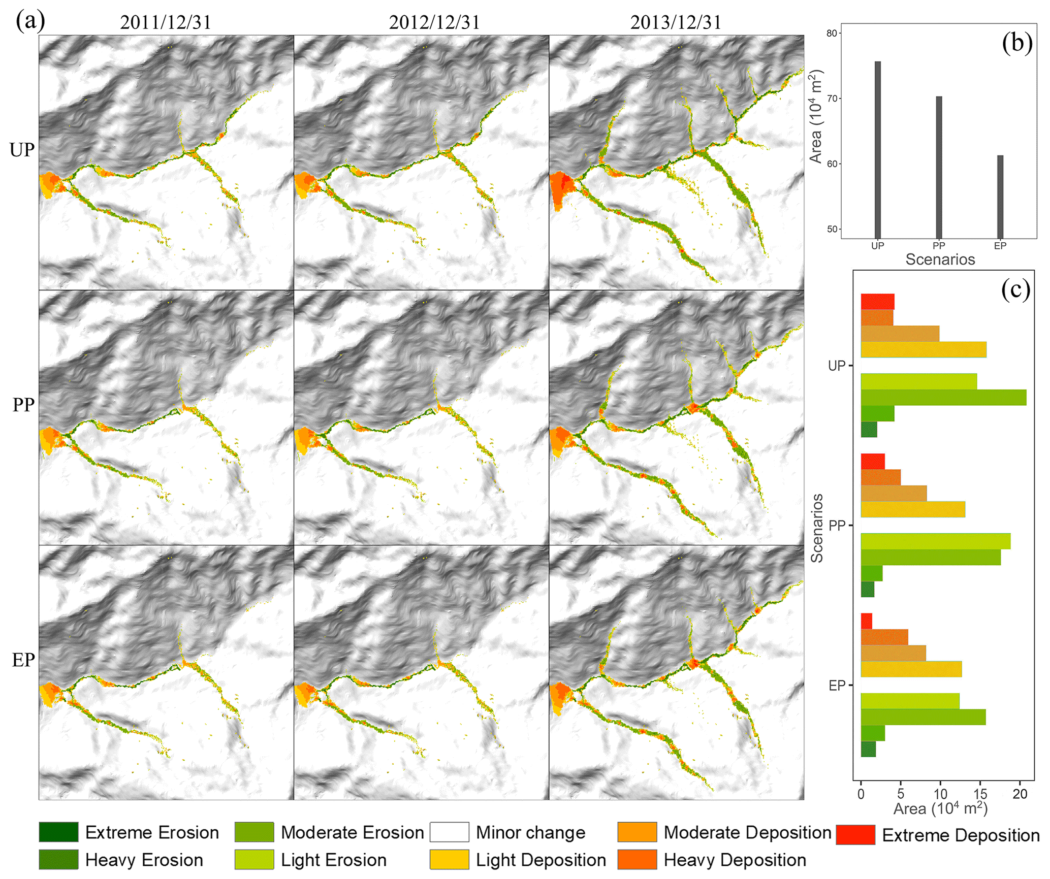
Figure 6 (a) Simulated geomorphic changes over time for the three scenarios, (b) the affected area of deposition and erosion for the three scenarios and (c) the columnar distribution of different erosion and deposition levels.

The total area of erosion and deposition in the three scenarios is calculated to compare the impact of sediment transport (Fig. 6b). The affected area in Scenario UP is approximately 0.76 km² (5.4 % of the total catchment), which is larger than that in Scenario PP (0.70 km², 5.0 % of the whole catchment), and the affected area decreases to 0.61 km² (4.4 % of the total catchment) in Scenario EP. The total area of erosion and deposition decreases gradually with more controlling measures established in this study.

Figure 6c compares the extent of geomorphic changes in three situations using the ranges that varied in depth. The areas of light and moderate erosion are greater than the areas of extreme and heavy erosion in all three scenarios. The zone of each erosion degree in UP is more extensive than that in PP, followed by that in EP. In addition, the greater the deposition depth is, the smaller the area of deposition. In particular, the extreme deposition area is greater than the area of heavy deposition in the UP scenario. Further analysis shows that the extreme, moderate and light deposition areas decrease in the order of UP, PP and EP. The heavy deposition area shows the opposite trend, mainly attributed to the check dams and slope protection with vegetation.

4.3 Details of key locations

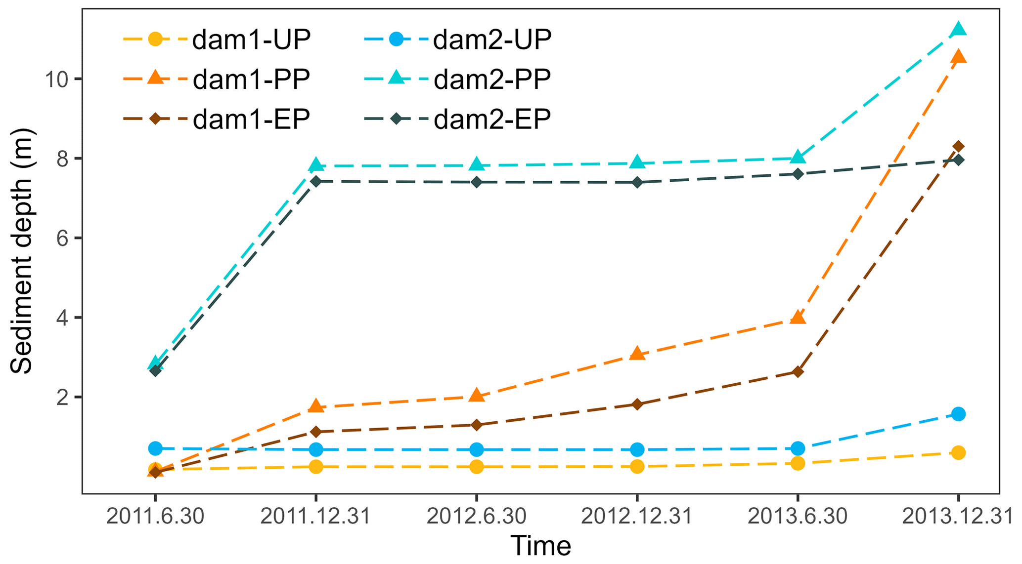
As shown in Fig. 7, the control measures and surroundings for the three scenarios are further investigated. Behind the two dams upriver in Scenarios PP and EP, the evident orange clusters indicate deposition. In contrast, these locations are dominated by erosion, shown in green, in scenario UP. Further analysis of the sediment depth shown in Fig. 8 shows that the deposited depth behind the dams in Scenario EP is lower than that in Scenario PP. Additionally, in Scenario PP, sediment trapped by dam 1 is less than that of dam 2, but both have deposition thicknesses of more than 10 m, which exceed the dams' heights (dam 1's height is 10 m, dam 2's height is 9 m). For the simulation results in Scenario EP, the values of deposition depth behind the two dams are nearly 8 m, which is lower than the dams' heights.

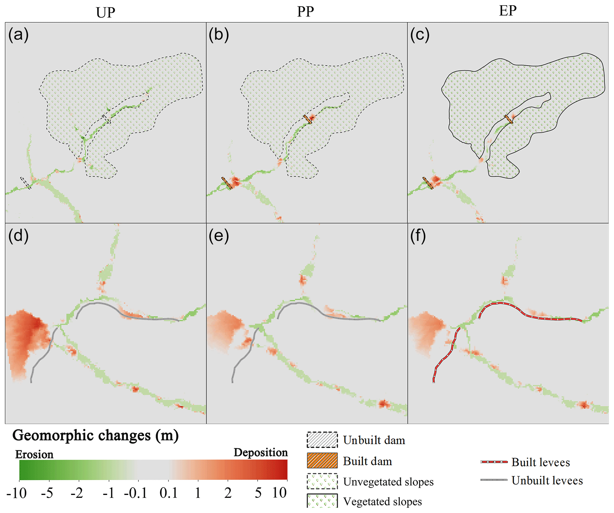
Figure 7 Geomorphic changes at key locations of the simulation results for the UP, PP and EP scenarios. (a, b, c) The upriver extent containing dam 1, dam 2 and the vegetated slopes. (d, e, f) The downriver extent containing levees.

Figure 8 The depth of deposited sediment in the dams' placements.

The additional ecological protection measure alters the material produced from the upriver tributary gullies. A sediment volume of 14.4×10⁴ m³ is transported from the vegetated slopes in the EP scenario (solid lines in Fig. 7). A total of 27.1×10⁴ and 16.9×10⁴ m³ of loose material is produced in the same region without ecological protection in Scenarios UP and PP, respectively. The vegetated slopes enhance sediment conservation in conjunction with dam 1. Compared with the deposition in UP and PP without levees in the downriver area (shown in the bottom row of Fig. 7), the levees in EP block debris in the bend of the channel and play an essential role in protecting the residents and cultivated land behind the levees.

4.4 Effectiveness assessment of the intervention measures

Figure 9 shows the erosion and deposition volumes in the source, transitional and deposition areas and compares the conservation ability (Ca) in each scenario. For all three scenarios, the deposition volume in the source area is less than that in the transitional area, and the largest amount of sediment accumulates in the deposition area. Regarding the eroded sediment, the largest volume is in the transitional area, followed by the transitional area, and the source area presents the lowest volume. Moreover, sediment transport is best controlled in the deposition area and worst contained in the source area under any intervention conditions.

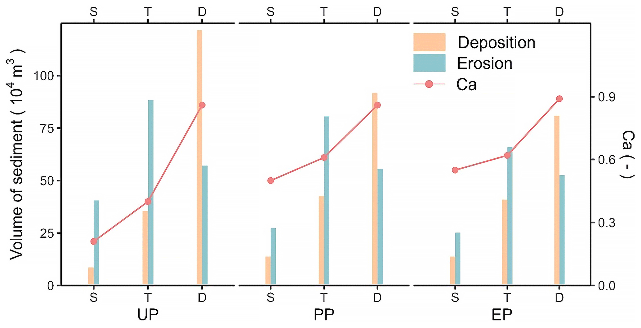
Figure 9 The volumes of sediment and the conservation ability (Ca) in the three areas for each scenario (S: source area, T: transitional area, D: deposition area).

Compared with the Ca of the source area in Scenario UP, the value increases by 138.1 % in Scenario PP, which is attributed to dam 1. Likewise, dam 2 in the transitional area effectively reduces sediment loss, which is reflected by a 52.5 % increase in Ca. Furthermore, the mitigation measures in Scenario PP with vegetated slopes and levees in Scenario EP act best. The conservation ability in the source area increased by 161.9 % due to the dam retainment and slope protection with vegetation, and the levees helped increase the Ca by 3.49 % in the deposition area.

The cumulative sediment yield time series for each scenario and the relative efficiency of scenarios UP and EP are presented in Fig. 10b and a, respectively. The steep curve of the output cumulative sediment indicates a significant increase in deposition. Three increasing stages are consistent with the rainfall intensity in the three monsoons (May–September). The total sediment output in UP is the largest at $\sim \mathrm{30.4}\times {\mathrm{10}}^{\mathrm{4}}$ m³, followed by the sediment yield of PP at 26.3×10⁴ m³, and EP produced the least material at 19.3×10⁴ m³.

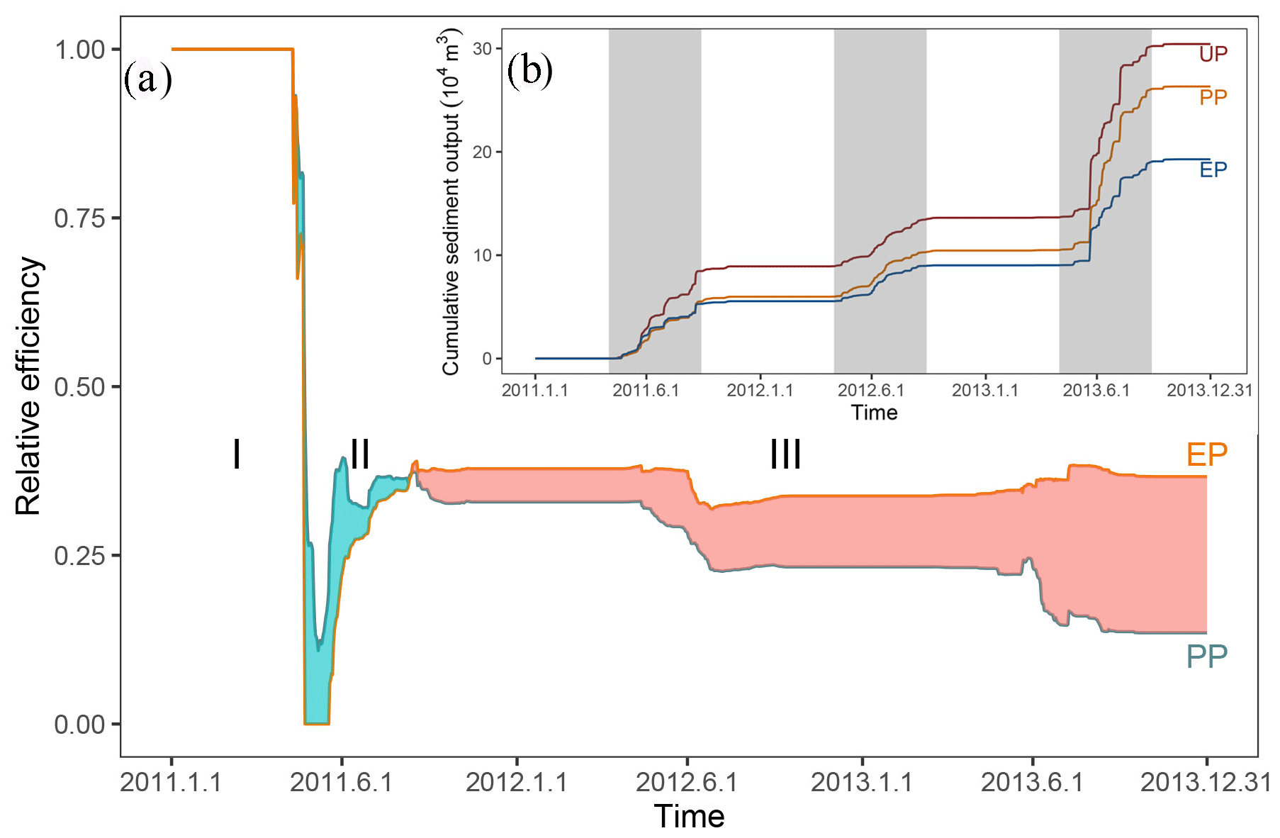
Figure 10 (a) Relative efficiencies of Scenarios UP and EP compared with that of Scenario UP (cyan shading represents when PP is more effective than EP and red shading represents the opposite). (b) Cumulative sediment yield over time (grey region highlighting three monsoons).

The relative efficiency over the period of controlling measures by human intervention in PP and EP (Fig. 10a) indicates three distinct stages. Stage I shows that the intervention measures in both scenarios completely prevent sediment transport. Later, stage II shows a peculiar period when the effect of enhanced protective measures in EP is less than that in PP through repeated experiments. In stage III, the relative efficiency of the intervention measures in EP is greater than that in UP, which achieves the long-term effect and stable conservation of solid material.

5 Discussion

5.1 Model calibration and uncertainty

Calibration and uncertainty analysis are important issues in the CAESAR-Lisflood (C-L) simulation of the geomorphic response to intervention measures based on the CA framework (Yeh and Li, 2006). A preliminary calibration was carried out in our study by reproducing the geomorphic changes and water depth driven by an extreme rainfall event that occurred in 2018. The results (Fig. S3) demonstrated that the C-L model can well replicate the flash flood event using the initial conditions and model parameters. The calibration of the geomorphic response to the intervention measures was derived from a direct comparison between the model results and observed measurements (Figs. 4 and 5). As a result, the simulated water discharge was greater than the measured discharge but on the same order of magnitude. Moreover, the errors of erosion and deposition depth between the simulation in Scenario PP and photographic evidence at three locations were less than 20 %. These results suggest the robustness of the model settings and parameterisation.

The source of uncertainty is mainly from the model parameters and driving factors. Skinner et al. (2018) provided a detailed sensitivity analysis of C-L, indicating that the sediment transport formula significantly influences a smaller catchment modelled by 10 m grid cells. The sediment transport law and the Wilcock and Crowe equations (Wilcock and Crowe, 2003) have been proved suitable in the Xingping valley (Xie et al., 2018, 2022a, b; Li et al., 2020). Nevertheless, the empirical models of sediment transport overpredict bedload transport rates in steep streams (gradients greater than 3 %) (D'Agostino and Lenzi, 1999; Yager et al., 2012). Additionally, the input hourly rainfall data downscaled from the daily sequence is an unrealistic situation. Various sediment transport equations and downscaled hourly rainfall data need to be tested in the C-L model to further decrease uncertainty.

5.2 The intervention effects

In this study, various measures were taken to represent three intervention scenarios with the goal of controlling sediment transport. The C-L model simulated the geomorphic responses to intervention measures and suggested the considerable influence of intervention measures on spatial modifications and sediment yield. The intervention measures lead to reductions in the total affected area (7.9 %–19.7 %) and lower sediment yields (16.7 %–36.7 %), as demonstrated by the overall evidence (see Figs. 6 and 10). The model's prediction of the overall catchment-scale dynamics in response to extreme events is in line with the viewpoints of other authors (Chen et al., 2023, 2015; Lan et al., 2020).

The mitigation measures change the soil conservation ability considerably in the subregions including source area, transitional area and deposition zone, especially in the source area. Compared to the other two subregions, we postulated that the decreased erosion in the source area was caused by the interactions of loose material and topographic constraints. First, most of the loose solid material triggered by the strong earthquake has stabilised since the 2008 debris flow (details in Table S1). Second, the long and deep gullies are mainly located in the transitional area (Yaogouli, Shicouzi, Yangjiashan) and deposition area (Qinggangping). These gullies provide a greater sediment supply than the source area. As shown in Fig. S4, the movement of the material occurs mainly in the branch valleys in the transitional and deposition zones.

Moreover, morphological changes and the ability of soil conservation in the three scenarios show the unique role played by different intervention measures. For example, check dams are most effective in blocking sediment, and vegetated slopes can further strengthen the conservation ability. The synergetic effect of the combination of check dams and vegetation coverage increases the soil conservation ability by more than twofold. The levees can pose a discernible impact on sediment conservation with specific object-oriented protection.

The effectiveness of mitigation measures decreases over time. We performed an additional 10-year experiment to reveal the declining trend over an extended period. We randomly selected one of the 50 repeated rainfall datasets (year 2016–year 2025) downscaled by Li et al. (2020), which were generated from the NEX-GDDP product (spatial resolution: $\mathrm{0.25}{}^{\circ }\times \mathrm{0.25}{}^{\circ }$, temporal resolution: daily) under the RCP 4.5 emission scenario. The extracted rainfall sequence was then input into the C-L model to simulate the effectiveness of the three intervention scenarios. The result (Fig. 11) illustrates that stage III (the stable stage that started on the 161st day, in which Scenario EP's intervention measures were more effective) lasted longer than stages I and II. The relative effectiveness in both the PP and EP scenarios decreased gradually, while the curve fell faster in the PP scenario (slope: $-\mathrm{1.65}\times {\mathrm{10}}^{-\mathrm{5}}$) than in the EP scenario (slope: $-\mathrm{1.31}\times {\mathrm{10}}^{-\mathrm{5}}$).

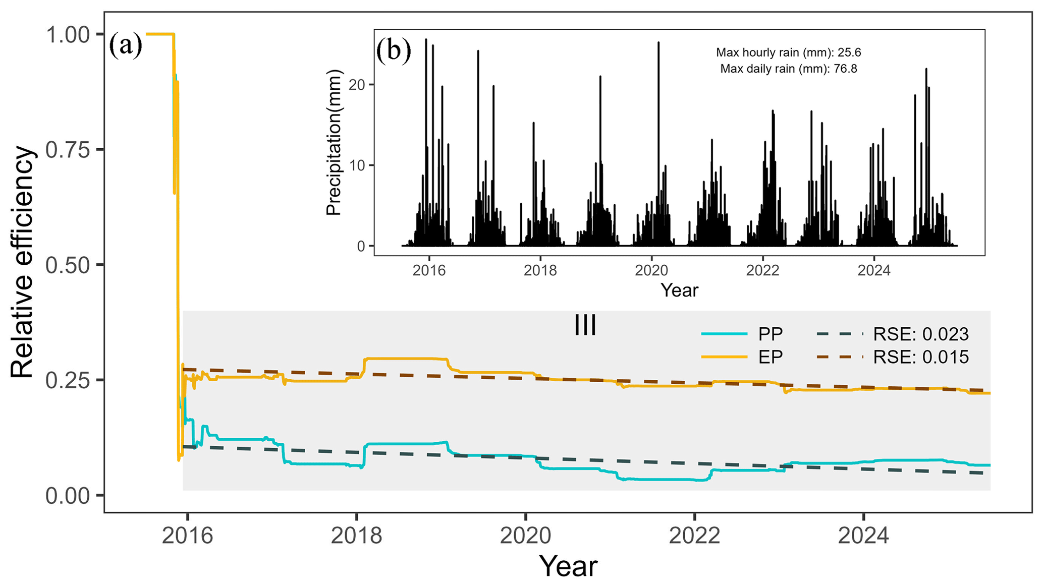
Figure 11 Rainfall input over 10 years and relative efficiency of sediment intervention measures. (a) Relative efficiency changes over 10 years (the grey region highlights stage III, and the dashed lines indicate the linear fitting curves); (b) Rainfall downscaled from the NEX-GDDP (NASA Earth Exchange Global Daily Downscaled Projections) product.

The storage capacity of the check dams decreases with sediment accumulation, and this decrease necessarily leads to a gradual reduction in intervention effectiveness. However, slope protection with vegetation remains operationally effective in reducing sediment transport by stabilising topsoil over the period when the role of dam reservoirs gradually fails due to the lack of dredging work. Therefore, the vegetation protection strategy is vital for “green development” to reduce sediment loss but requires further efforts.

5.3 Limitations and applications

We built the check dams and levees in our simulations by increasing the elevation in specific locations where they could not be eroded (see https://sourceforge.net/projects/caesar-lisflood/, last access: 30 March 2023), which has been proved experimentally feasible (Poeppl et al., 2019; Gioia and Schiattarella, 2020). The check dam and levee bodies embedded in the model were not broken or weakened over time so that the simulation result could underestimate the geohazard risks. Considering the complexity of the geohazard mechanism, the above-mentioned tools cannot simulate the occurrence process of geohazard chain links. They ignore the possible instantaneous damage to the environment and facilities downstream.

The methods applied in the study further demonstrate that the C-L is an effective tool for understanding short–medium-term or long-term geomorphic changes (Ramirez et al., 2022; Li et al., 2020; Coulthard et al., 2012a) and testing the effectiveness of intervention measures under different scenarios. Our simulations indicate that the mitigation measures in this study are effective, especially the combination of check dam and vegetated slopes in the upstream area, which could help decision makers optimise the management strategies to control mountain disasters. Though geotechnical engineering is a mature technology that can effectively prevent geohazard occurrence (Cui and Lin, 2013), it has disadvantages such as extensive cost and the difficulty of maintenance. In green development, the planting and maintenance of vegetation cover can effectively prevent erosion by strengthening topsoil and absorbing excess rainwater via roots (Reichenbach et al., 2014; Stokes et al., 2014; Forbes and Broadhead, 2013; Mickovski et al., 2007). Alternatively, these methods can be used to study the impact of tree planting patterns on sediment dynamics.

6 Conclusions

In this study, scenarios involving check dams, vegetated slopes and artificial barriers were simulated using the C-L model to outline the erosion and deposition areas, measure the impacts of sediment blocking and retention, and thus examine how vegetated slope help stabilise slopes. Four key findings were obtained. First, the geotechnical engineering used for controlling sediment transport are efficient, and their performance in protecting the fragile environment can be improved by integrating with other intervention measures, such as ecological engineering and artificial barriers. Second, the effectiveness of mitigation measures decreases over time. Third, the characteristics of the sediment transport patterns are considerably altered due to the intervention measures. The stabilising sediment ability in the source area increased by 161.9 % with the additional effect of slope protection with vegetation. To sum up, the present intervention measures need to be refined with regular dredging works to maintain the effectiveness of reducing sediment transport.