the Creative Commons Attribution 4.0 License.
the Creative Commons Attribution 4.0 License.
 | 05 Apr 2023
Heat wave monitoring over West African cities: uncertainties, characterization and recent trends
Cedric Gacial Ngoungue Langue
Christophe Lavaysse
Mathieu Vrac
Cyrille Flamant
Heat waves can be one of the most dangerous climatic hazards affecting the planet, having dramatic impacts on the health of humans and natural ecosystems as well as on anthropogenic activities, infrastructures and economy. Based on climatic conditions in West Africa, the urban centres of the region appear to be vulnerable to heat waves. The goals of this work are firstly to assess the potential uncertainties encountered in heat wave detection and secondly to analyse their recent trend in West Africa cities during the period 1993–2020. This is done using two state-of-the-art reanalysis products, namely the fifth-generation European Centre for Medium-Range Weather Forecasts (ECMWF) reanalysis (ERA5) and Modern-Era Retrospective analysis for Research and Applications (MERRA), as well as two local station datasets, namely Dakar–Yoff in Senegal and Aéroport Félix Houphouët-Boigny, Abidjan, in Côte d'Ivoire. An estimate of station data from reanalyses is processed using an interpolation technique: the nearest neighbour to the station with a land sea mask ≥0.5. The interpolated temperatures from local stations in Dakar and Abidjan show slightly better correlation with ERA5 than with MERRA. Three types of uncertainty are discussed: the first type of uncertainty is related to the reanalyses themselves, the second is related to the sensitivity of heat wave frequency and duration to the threshold values used to monitor them, and the last one is linked to the choice of indicators and the methodology used to define heat waves. Three sorts of heat wave have been analysed, namely those occurring during daytime, nighttime, and both daytime and nighttime concomitantly. Four indicators have been used to analyse heat waves based on 2 m temperature, humidity, 10 m wind or a combination of these. We found that humidity plays an important role in nighttime events; concomitant events detected with wet-bulb temperature are more frequent and located over the northern Sahel. Strong and more persistent heat waves are found in the continental (CONT) region. For all indicators, we identified 6 years with a significantly higher frequency of events (1998, 2005, 2010, 2016, 2019 and 2020), possibly due to higher sea surface temperatures in the equatorial Atlantic Ocean corresponding to El Niño events for some years. A significant increase in the frequency, duration and intensity of heat waves in the cities has been observed during the last decade (2012–2020); this is thought to be a consequence of climate change acting on extreme events.
- Article
(4884 KB) - Full-text XML
-
Supplement
(6033 KB) - BibTeX
- EndNote


Since the industrial revolution, the Earth has experienced global warming related to human activity (Hartmann et al., 2013; Intergovernmental Panel on Climate Change – IPCC – report 2021; Eyring et al., 2021). The last report of the IPCC shows that this warming will exceed 1.5 ∘C with respect to the IPCC baseline of 1850–1900 under different Shared Socioeconomic Pathways (SSPs) in 2100 if the rate of greenhouse gas emissions is not reduced. This warming climate not only contributes to the occurrence of extreme events but also tends to reinforce their intensity (Fischer and Schär, 2010; Engdaw et al., 2022; IPCC report 2021). Heat waves appear as one of the most dangerous climatic hazards affecting the planet due to their impacts on several sectors (Perkins, 2015). The health sector is the most affected; heat waves act on the thermal comfort of the body, leading to an increase in morbidity and respiratory and cardiovascular diseases among the most vulnerable population (children and the elderly) (e.g. Huynen et al., 2001; Braga et al., 2002; Hajat et al., 2007; Kovats and Hajat, 2008; Anderson and Bell, 2009; Gasparrini and Armstrong, 2011; Rocklöv et al., 2014). Heat waves are “silent killers” because their impacts on human health are not usually instantaneous (Loughnan, 2014). In 2003, an intense heat wave occurred in France, killing more than 14 000 people (Fouillet et al., 2006). During this event, temperatures sometimes reached 37 ∘C, a record since 1950. This event was very persistent and lasted 2 weeks in France. In addition to this event, the Russian heat wave in 2010 caused numerous destruction (dysfunction of railway stations, interruption of energy production) and more than 11 000 deaths (Shaposhnikov et al., 2014). Temperatures sometimes reached 38 ∘C and generated huge fires in the neighbouring regions of Moscow and a high concentration of carbon monoxide in the troposphere. In April 2010, northern Africa was affected by a severe heat wave with daily maximum temperatures frequently exceeding 40 ∘C and daily minimum temperatures over 27 ∘C for more than 5 consecutive days (Largeron et al., 2020).
Heat waves are natural disasters often associated with an increase in daytime and/or nighttime temperatures. More generally, they are defined as a period of consecutive days during which temperatures are much hotter than normal. There is no universal formulation describing a heat wave; however a definition could be made according to the context of the study (health, environment, infrastructure, agriculture, energy supply). From a physiological point of view, the severity of a heat wave is measured through its duration and intensity.
West Africa experiences a very hot and dry climate over the Sahel region and a hot and humid climate over the Guinea coast. The climatic conditions over West Africa make the region vulnerable to heat waves when it comes to not only the health of humans and natural ecosystems but also agriculture. Many studies on heat waves have been carried out in Europe. However, heat waves in Africa are still not well documented. Moron et al. (2016) analysed the trends of extreme temperatures in northern tropical Africa from observations and reconstructed data. They show that heat wave indices over the region were highly correlated with the El Niño–Southern Oscillation indices (ENSO). Barbier et al. (2018) investigated the intraseasonal variability of large-scale heat waves during spring using the Berkeley Earth Surface Temperatures (BEST) gridded dataset and the following reanalyses: the European Centre for Medium-Range Weather Forecasts interim reanalysis (ERA-Interim), Modern-Era Retrospective analysis for Research and Applications (MERRA; see Sect. 2.2 for more details), and the National Centers for Environmental Prediction Reanalysis 2 (NCEP-2). They defined heat waves using anomalies of minimum/maximum values of the 2 m temperature. They found some discrepancies in the characteristics, variability and climatic trends of heat waves in the different products. Largeron et al. (2020) analysed the April 2010 heat wave in North Africa using both the BEST dataset and climate simulations from the atmospheric component of the Centre National de Recherches Météorologiques (CNRM) climate model. They showed a strong link between heat waves over the Sahara and the incoming heat surface fluxes. Another important result of this work is the radiative effect of water vapour on minimum temperatures during the heat wave period. This can lead to extreme heat conditions during the night and the death of elderly people. Guigma et al. (2020) analysed the characteristics and thermodynamics of Sahelian heat waves using different thermal indices based on temperature, wind speed and relative humidity derived from fifth-generation ECMWF reanalysis (ERA5; see Data section for more details). They found that most of the regions in the Sahel experience on average one or two heat waves per year with a duration of 3–5 d and severe magnitude. They have also shown that the eastern Sahel experiences more frequent and longer events. They identified heat advection and the greenhouse effect of moisture as the main drivers of Sahelian heat waves. Some of the previous studies conducted over the Sahelian band only use the daily maximum and minimum temperatures (e.g. Moron et al., 2016; Barbier et al., 2018) for the detection of heat waves, thereby ignoring the potential influence of humidity and wind speed. Others take into account the effect of humidity in the heat wave definition (e.g. Guigma et al., 2020), but information about the interannual and seasonal variability of events detected is missing, even though this is very important for policymakers and governments to take into account in order to develop early alert systems. Recently, Engdaw et al. (2022) studied the trends of heat waves over Africa during the period 1980–2018 using observations from the Climate Research Unit Time-Series version 4.03 (CRU TS4.03) and BEST datasets as well as the following reanalysis datasets: ERA5, MERRA-2 and the Japanese Meteorological Agency’s 55-year reanalysis (JRA-55). They highlighted large differences in both the trend and the temporal evolution of heat wave indices between the different reanalyses. They found a peak of heat over northern and western Africa in 2010 as well as in 2016 over eastern and southern Africa. They noticed significant warming and an increase in heat wave occurrence in all the regions in Africa. However, Engdaw et al. (2022) focused only on dry heat waves over a large domain of West Africa (10∘ S–15∘ N, 20∘ W–20∘ E); the duration of heat waves was not addressed and nor was the evolution of wet heat waves.
The most lethal heat waves are due not only to high temperatures but also to the effect of humidity (Steadman, 1979a, b); hot and humid conditions (as is the case in coastal regions) can be more dangerous than equivalently hot but dry conditions (Wehner et al., 2017). Wet heat waves, which are the most dangerous for human health, were not investigated in previous works. Following Steadman (1979a, b), one can legitimately wonder about the effect of humidity on the frequency of heat waves and on the evolution of humid heat waves in West African cities. Based on previous studies, many definitions of heat wave have been proposed, leading to different results. Indeed there is no universal definition of a heat wave; depending on the research applications, some indicators and definitions can be adopted. Thus, we can question the potential sources of uncertainty found in heat wave analysis.
The goals of this paper are (i) to highlight the potential uncertainties encountered in the heat wave detection process and (ii) to analyse the recent trend and characteristics of dry and wet heat waves over a selection of West African cities grouped into climatic regions. To achieve these objectives, we first assess the biases in the reanalyses (ERA5, MERRA) using ERA5 as a reference; then, a sensitivity analysis of the frequency of heat waves with respect to the threshold values, indicators and methods applied to define heat waves is addressed. Finally, we assess the spatial and temporal variability (seasonal and interannual) of heat waves and their characteristics in different climatic regions over West Africa.
The remainder of this article is organized as follows: in Sect. 2, we present the regions of interest and the data used for this work; the description of the methodology is also provided. Section 3 contains the main results of this study following the methodology described in Sect. 2. In Sect. 4, the uncertainty in the reanalyses and the origin of coastal heat waves are discussed. Section 5 provides a conclusion and some perspectives for future works.
2.1 Region of interest
The current study is conducted over West Africa, which is located over the domain 5–20∘ N, 15∘ W–10∘ E, and spans the Atlantic coast to Chad and the Gulf of Guinea to the southern fringes of the Sahara (Fig. 1). The climate in West Africa is mostly influenced by the West African monsoon flux, which governs the rainy season and thus the rain-fed agriculture. The West Africa region has a semi-arid and hot climate with a dry season (Köppen classification BSh or BWh). This climate corresponds to an alternation between a short wet season and a very long dry season. The West Africa region shows high climate variability at a regional and local scale. In this study, we are interested in the coastal and continental parts of West Africa. We have therefore identified three regions based on their location and climate variability on which we have conducted our analyses. The choice of these regions is coherent with Moron et al. (2016), who used a hierarchical-clustering approach to define some city blocks over West Africa. The 15 cities investigated here were classified into the three following regions:
-
continental zone (CONT hereafter) including the cities of Bamako, Ouagadougou and Niamey (Fig. 1);
-
coastal Atlantic zone (ATL hereafter) including the cities of Dakar, Nouakchott, Monrovia and Conakry (Fig. 1);
-
coastal Guinean zone (GU hereafter) including the cities of Yamoussoukro, Abidjan, Lomé, Abuja, Lagos, Accra, Cotonou and Douala (Fig. 1).
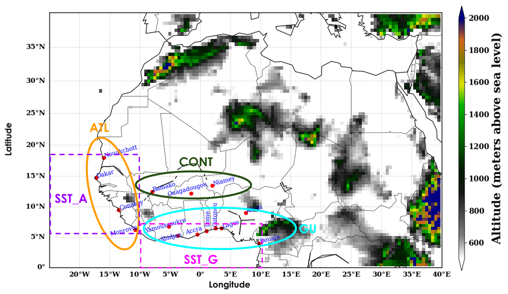
Figure 1Topographic map of West Africa using ERA5 elevation data. The circles on the map represent the different climatic zones: ATL (coastal Atlantic zone), CONT (continental zone) and GU (coastal Guinean zone). The two boxes named SST_A and SST_G represent the boxes used to analyse the links between sea surface temperature (SST) and heat waves for the ATL and GU regions respectively. The y and x axes represent the latitude and longitude respectively. The colour bar shows the elevation in metres over the region.
The CONT and GU regions are very similar to the clusters found by Moron et al. (2016) (see figure under the title “Clusters membership” in Moron et al., 2016). The ATL region is a specific case because not all cities belonging to the region are present in the clusters defined by Moron et al. (2016). Therefore, we analysed the spatial variability of heat wave characteristics for each city. In this way, we found a consistent pattern across cities (see Fig. S1 in the Supplement for maximum T2 m values using the 90th percentile as a threshold), and we grouped them to form the ATL block.
2.2 Data
Reanalysis products are often taken as an alternative solution to observational weather and climate data due to availability and accessibility problems, particularly in data-sparse regions such as Africa (Gleixner et al., 2020). In this work, to access information with a regular spatial grid and a large horizontal coverage, we used two state-of-the-art reanalysis products: the fifth-generation European Centre for Medium-Range Weather Forecasts (ECMWF) reanalysis (ERA5; Hersbach et al., 2020) and the Modern-Era Retrospective analysis for Research and Applications, version 2 (MERRA-2; Gelaro et al., 2017), from the National Oceanic Atmospheric Administration (NOAA) (in the following, we will use “MERRA” to refer to MERRA-2). ERA5 reanalysis has a native spatial resolution of 0.28125∘ (∼31 km) with 137 hybrid sigma–pressure levels from the surface up to 80 km, yet downloaded data are interpolated to a regular latitude–longitude grid of . ERA5 is produced using 4D-Var data assimilation and the Cycle 41r2 (Cy41r2) of the ECMWF Integrated Forecasting System (IFS), which was operational in 2016. MERRA reanalysis has a spatial resolution of with 42 standard pressure levels. MERRA uses an upgraded version of the Goddard Earth Observing System model version 5 (GEOS-5) data assimilation system and the Gridpoint Statistical Interpolation (GSI) analysis scheme of Wu et al. (2002). MERRA is produced using a 3D-Var data assimilation algorithm. These two reanalyses datasets can be accessed through the Climserv database from the Institut Pierre-Simon Laplace (IPSL) server. To be consistent in our analyses, we transformed the spatial resolution of MERRA from to to match the one of ERA5; this is done using a first-order conservative interpolation. We use hourly data covering the period from 1 January 1993 to 31 December 2020 for both ERA5 and MERRA. Our choice of ERA5 and MERRA to conduct this study is supported by some previous work showing that these two reanalyses included among the most relevant used in African regions (e.g. Barbier et al., 2018; Ngoungue Langue et al., 2021; Engdaw et al., 2022). As the main objective here is to process heat wave detection, we focus on atmospheric variables at the surface such as 2 m temperature (T2 m), 2 m relative humidity (RH), 2 m dewpoint temperature, 2 m specific humidity, 10 m wind components, and water vapour pressure (e) from which wet-bulb temperature (Tw) and apparent temperature (AT; McGregor et al., 2015) were derived. These atmospheric variables have a significant impact on human thermal comfort (McGregor et al., 2015). Daily minimum and maximum values were calculated for T2 m, Tw, AT and the universal thermal comfort index (UTCI; Di Napoli et al., 2021). AT is similar to the heat index developed by Steadman (1984). The climate variables e, Tw, AT and RH were calculated using the following formulas:
(Buck, 1981; Alduchov and Eskridge, 1996),
(Stull, 2011) (RH is given as a percentage, for example 32 for RH =32 %),
(McGregor et al., 2015).
RH is computed differently based on the variables available in the products. The first formula is used to compute RH in ERA5, and the second is used for MERRA.
(August, 1828; Magnus, 1844; Alduchov and Eskridge, 1996),
(https://earthscience.stackexchange.com/questions/2360/how-do-i-convert-specific-humidity-to-relative-humidity, last access: 3 April 2023), where a=17.625, b=243.04, A=0.151977, B=8.313659, C=1.676331, D=0.00391838, E=0.023101, F=4.686035 and T0=273.16 K. T (∘C), Td (∘C), T0 (K), p (hPa), Ws (m s−1) and q are the ambient temperature, dewpoint temperature, reference temperature, pressure, wind speed and specific humidity respectively.
The land sea mask dataset used in this work was derived from ERA5 reanalysis; it can be accessed on the Copernicus Climate Data Store (CDS). T2 m daily maximum and minimum observations at Dakar–Yoff station in Senegal and Aéroport Félix Houphouët-Boigny (FHB) station in Côte d'Ivoire were used to evaluate our interpolation method. This is due to the fact that we do not have access to other station data in these regions. The data from Dakar–Yoff extend from 1 January 1973 to 31 December 2018 and contain almost 16 % missing values, and the data from Aéroport FHB extend from 1 January 2005 to 31 December 2017 and contain 0.35 % missing values. These data were provided by colleagues from the Agence Nationale de l'Aviation Civile et de la Météorologie (ANACIM) for the Dakar–Yoff station and from the Institut des Géosciences de l'Environnement (IGE) for the Aéroport FHB station.
2.3 Methods
2.3.1 Estimation of atmospheric variables at the scale of cities
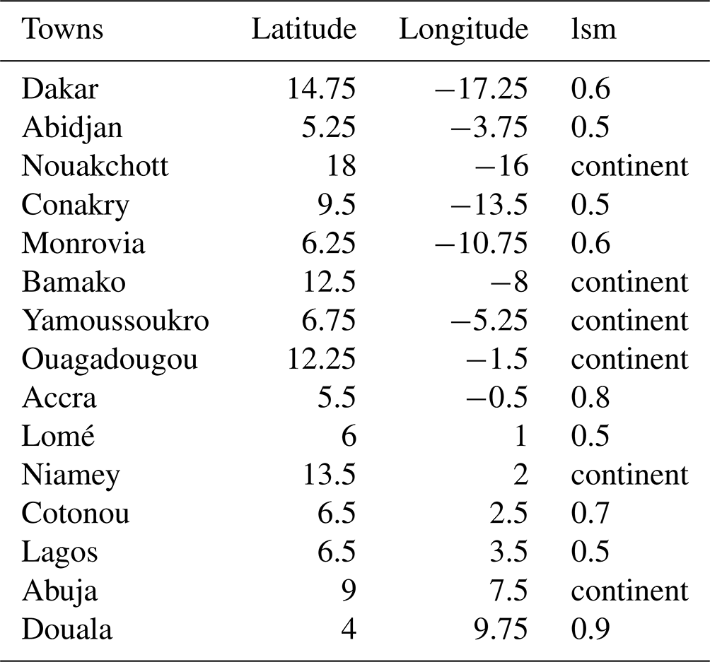
Reanalysis datasets used for weather studies are generally run at a global scale; therefore information at a local scale is missing in many regions; this is a critical issue in regions where there is a lack of observation stations as is the case for African cities. To overcome this problem, downscaling methods can sometimes be used. In this work, we study phenomena at the scale of the cities, and reanalyses (ERA5 and MERRA) have too coarse a spatial resolution. The scales of the reanalyses are more representative of the spatial variability of a heat wave occurring in a city than at an isolated local station. Nevertheless, some validation of the test stations needs to be done, in particular to find the best interpolation technique to estimate local temperatures from the reanalyses. This is especially important over the coastal regions. Indeed, most of the cities used in this study are located along the coast and influenced by the ocean air masses (see Fig. 1). The evaluation of the spatial variability of the correlation between the local-scale variable (station) and reanalyses (ERA5) for T2 m, for example, showed high correlation values over the continent (Fig. S2) (Dakar, Abidjan). This suggests that the station data are well correlated with ERA5 grid points which are located on the continent; it is therefore necessary to know whether an ERA5 grid point is over the continent or not before applying an interpolation technique. To estimate the proportion of land on a grid point, we used the land sea mask (lsm) with values ranging from 0 to 1. The land sea mask is a measure of the land occupation on a grid point. An lsm of 0 means no land (a grid point located in the ocean), and an lsm of 1 means that the model cell is fully covered by land. Therefore, to estimate the climate variables over the cities from reanalyses, we use the nearest grid point of reanalyses to the station which satisfies an lsm equal to or greater than 0.5 (see Table 1 for lsm values of all the cities considered in this study). This approach was chosen after evaluating different methods such as the following (see Fig. S3a for more details):
-
a bilinear interpolation using the four nearest grid points of reanalyses around the station (panels a and d in Fig. S3a),
-
a linear gradient approach which considers the gradient of temperature constant between two grid points based on a linear interpolation with a condition placed on the lsm value (≥0.5) (panels c and f in Fig. S3a),
-
the selection of the nearest grid point of reanalyses from the station with different values of lsm (≥0.5, 0.75 and 1; we show only results for lsm ≥0.5) (panels`b and e in Fig. S3a),
-
a dynamical interpolation approach taking into account the effect of winds (not shown).
Table 1Land sea mask (lsm) of West African towns used in this study.
The interpolation method was applied to ERA5 and MERRA, and the resulting estimated data were compared to the station data by correlation analysis. We found that ERA5 appears to be slightly better than MERRA at both stations (Dakar and Abidjan) for minimum and maximum T2 m values (Fig. S3b).
2.3.2 Heat wave detection
Heat waves are usually defined as consecutive days of extremely hot temperatures above a threshold temperature value (e.g. Tan et al., 2010; Gasparrini and Armstrong, 2011; Perkins and Alexander, 2013; Wang et al., 2019). Many factors can affect the definition of a heat wave, including the end-user sectors (human health, infrastructures, transport, agriculture) and also the climatic conditions of the regions (Perkins and Alexander, 2013). Therefore, there is no universal and standard definition of a heat wave (Perkins, 2015; Oueslati et al., 2017; Shafiei Shiva et al., 2019). Different thresholds, duration and indicators contribute to the divergence in the definition of heat waves (Smith et al., 2013). Heat waves can be defined from daily meteorological variables such as daily raw temperature (Tmin, Tmean and Tmax) (e.g. Fontaine et al., 2013; Beniston et al., 2017; Ceccherini et al., 2017; Déqué et al., 2017; Batté et al., 2018; Barbier et al., 2018; Lavaysse et al., 2018; Engdaw et al., 2022), mean daily wet-bulb temperature (Yu et al., 2021) or heat stress indices (e.g. Robinson, 2001; Fischer and Schär, 2010; Perkins et al., 2012a; Guigma et al., 2020) using relative or absolute thresholds. The use of absolute thresholds is well suited to detecting heat waves during the year in regions where the seasonal cycle is well marked. In mid-latitudes for example, the seasonal thermal amplitude of T2 m is large, approximately 20 ∘C. In tropical regions this method is not suitable, since the seasonal thermal amplitude is strongly reduced (6 ∘C). Therefore, a relative threshold for heat wave detection is adopted in our study, since our region of interest is West Africa. Some authors use the daily anomalies of temperature to define heat waves (e.g. Stefanon et al., 2012; Barbier et al., 2018). Most of the previous studies are focused on daytime or nighttime heat waves, ignoring events which occur during the day and night concomitantly. This type of heat wave is very dangerous for human health because the body suffers from heat stress during the day and night (Lavaysse et al., 2018). In our case, we defined three methods to detect specific types of heat waves (namely those occurring during daytime, nighttime, and both daytime and nighttime concomitantly) using the daily minimum and maximum values of T2 m (, ), Tw (, ), AT (ATmin, ATmax) and UTCI (UTCImin, UTCImax) as indicators. The selected atmospheric variables have been used for heat wave detection in previous studies; they take into account some key parameters (air temperature, wind, humidity, radiant temperature) to assess the body heat stress, and they are easy to compute. The methods applied are defined below:
-
Method 1. A heat wave is defined as a consecutive period of at least 3 d during which the daily maximum value of an indicator exceeds the calendar 90th percentile of daily maximum values of the indicator computed over the whole period (see HW1 in Fig. 2). This approach is useful for monitoring daytime heat wave events. Daytime events will be more associated with incoming solar radiation.
-
Method 2. A heat wave is defined as a consecutive period of at least 3 d during which the daily minimum value of an indicator exceeds the calendar 90th percentile of daily minimum values of the indicator computed over the whole period (see HW2 in Fig. 2). This approach is useful for monitoring nighttime heat wave events. Nighttime events can be related to the moisture content of the region.
-
Method 3. A heat wave is defined as a consecutive period of at least 3 d during which daily minimum and maximum values of an indicator exceed the calendar 90th percentiles of daily minimum and maximum values respectively (see HW3 in Fig. 2). This method is most appropriate for extreme events that occur both during the day and at night and are very harmful for human health.
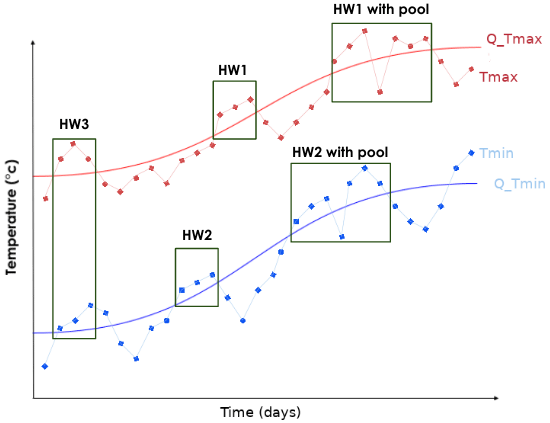
Figure 2Schematic illustration of heat wave detection process: HW1/HW2 represents heat waves associated with maximum/minimum temperature and HW3 is heat waves detected at the same time in maximum and minimum temperatures. The red/blue lines with squares are max/min daily temperatures. Solid red/blue lines are max/min thresholds. The x and y axes represent the time in days and the temperature in degrees Celsius respectively. The term “with pool” refers to the pooling of two (or more) events separated by 1 d below the daily threshold. This figure shows the different types of heat wave investigated in this work.
The 90th percentile is calculated for each calendar day of the year using an 11 d moving window centred on the day under study. The use of a moving window allows the seasonal cycle to be taken into account in the calculation of percentiles. The use of a relative threshold is more appropriate as it is easily replicable in other regions. When two heat wave events are separated by 1 d with an indicator value below the daily 90th percentile, they are pooled together to form a single event (see Fig. 2).
2.3.3 Heat wave characteristics
Once a heat wave is detected, some key characteristics are derived, namely duration and intensity. Some studies use the heat wave magnitude index daily (HWMId) to assess the severity of heat waves (e.g. Russo et al., 2016; Ceccherini et al., 2017). The HWMId focuses on strong heat waves; using this measure, the total intensity of all detected events cannot be assessed. In our study, the methodology applied to compute the duration and intensity of heat waves has been developed by Lavaysse et al. (2018) for monitoring extreme temperatures in Europe. We define the heat wave duration as the total number of hot days in heat waves. Hot days are heat wave days with daily values of the indicators above the daily thresholds. The heat wave duration is computed using the following expression:
where δj=1 if Tj> daily 90th percentile and δj=0 if Tj< daily 90th percentile and N represents the total number of heat waves per grid point and d the number of hot days in a heat wave. The Kronecker δj is used here because we pooled together heat waves separated by 1 d to form single events. For example, two heat waves of 4 and 3 d respectively separated by 1 d below the threshold will be counted as a single event with a duration of 7 d. For each block defined previously, the duration of heat waves is computed as the average of the duration of heat waves over the cities belonging to the same block. This also applies to the intensity.
The intensity of a heat wave has been defined as the sum of the daily exceedances of daily values of indicators above the climatological daily threshold in a sequence of hot days. This study is part of the Agence National de la Recherche STEWARd (STatistical Early WArning systems of weather-related Risks from probabilistic forecasts, over cities in West Africa) project, which focuses on the human impacts of climate extremes. Therefore, the climatological daily threshold is chosen to be constant over the whole period, and it is defined as the minimum of the daily climatology thresholds over the study period. This approach allows us to properly assess the severity of a heat wave and its potential human impacts. The expression of the intensity is given by
I1, I2 and I3 are intensities associated with HW1, HW2 and HW3 respectively. denotes daily maximum/minimum values of indicators at the grid point w. represents daily maximum/minimum threshold of the indicators at the grid point w. bool and bool are Boolean time series which contain 0 if the day is not part of a heat wave and 1 if the day is part of a heat wave for maximum and minimum daily values of the indicators respectively. boolmin–max,t,w is a Boolean time series which indicates 1 if the day is part of a heat wave detected simultaneously with both the minimum and the maximum values of indicators and 0 if this is not the case. Nd is the length in days of the study period. The mean duration and intensity are used to assess the severity of the heat wave.
2.3.4 Evaluation of the products using statistical metrics (hit rate, ACC, GSS)
Most regions in Africa suffer from a lack of observations due to a small number of available weather stations. To access information over a large domain, we use ERA5 and MERRA reanalysis datasets, which are very consistent in representing large-scale processes in the Saharan area (Ngoungue Langue et al., 2021). The coherence of reanalyses at a regional scale was assessed using statistical metrics such as the hit rate, the anomaly correlation coefficient (ACC) and the Gilbert skill score (GSS). The hit rate and GSS are used to evaluate hot days in the reanalyses.
Hit rate
The hit rate, also known as the “hit”, is a measure of the fraction of events detected in an evaluated dataset knowing that the events occur in the reference at the same time. It is given by the following formula:
TP denotes true positives, which are events correctly detected by the two datasets at the same time; FP denotes false positives, which are events not detected by the evaluated dataset but that occurred in the reference. Hit values range from 0 to 1; hit =1 means that all the events observed in the evaluated dataset occurred in the reference.
Previous work such as Olauson (2018) and Ramon et al. (2019) have shown that ERA5 provides a good representation of various near-surface meteorological variables including near-surface humidity and wind speed, in comparison to others reanalyses, including MERRA. Therefore for the computation of the hit, we chose ERA5 as the reference and MERRA as the evaluated dataset.
ACC
The ACC is similar to a linear correlation, the only difference being that it is calculated using the anomalies of the variables with respect to the climatology. This metric is stricter than the simple correlation and not sensitive to the seasonal cycle, which tends to increase the correlation between the products. ACC takes values between −1 and 1. ACC =1 indicates a perfect correlation between the products. For example, to compute the ACC between ERA5 and MERRA using the variable T2 m in this study, we firstly compute the anomalies between each reanalysis and their respective climatologies and then we compute the correlation between the resulting anomalies.
GSS
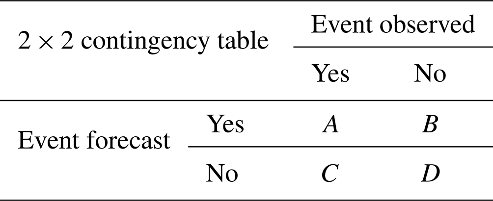
The GSS, known also as the equitable threat score (ETS), measures the fraction of observed events that are correctly predicted, adjusted for hits associated with random chance. The GSS does not take into account positive outcomes due to chance. It is stricter than the hit rate; the GSS takes values between and 1. GSS =0 indicates no skill or no correlation, while GSS =1 indicates perfect skill. Given a contingency table (see Table 2), the computation of the GSS is done by the following formula:
with CH given by
3.1 Uncertainties in the reanalysis products
The first step of this work consists in assessing the evolution of T2 m in the ERA5 and MERRA reanalyses. The climatological state (annual mean) of T2 m in ERA5 and MERRA has been evaluated over the West Africa region from 1 January 1993 to 31 December 2020 (Fig. 3a–b). Both reanalyses show very similar climatologies of T2 m: a north–south gradient of the temperature. The Sahel region appears to be warmer than the Guinean region; this is because of the advection of cold air coming from the Atlantic Ocean to the Guinea coast. This fresh air tends to cool down temperatures in this region. The bias between ERA5 and MERRA is computed using ERA5 as reference (Fig. 3c). MERRA shows a cold bias with respect to ERA5 over the Sahel region and Guinean zone except in some countries (e.g. Guinea-Bissau, Sierra Leone, Liberia) where we observe a hot bias. The biases between ERA5 and MERRA are around ±2 ∘C. The bias highlighted between ERA5 and MERRA is very significant for heat wave detection. Thereafter, we evaluated the temporal consistency between the two reanalyses by computing the ACC for T2 m, AT and Tw (see Fig. 3d–i). We observed a weak correlation over the south of the Sahel and Guinean region of around 0.5 (0.7) for maximum (minimum) values of T2 m and AT (see Fig. 3d–e and g–h). This could be explained by the presence of a strong diurnal cycle in the region associated with high variability during the day and less variability during the night. This will lead to high variability in the daily maximum values compared to the daily minimum values. Tw shows a uniform repartition of correlation between ERA5 and MERRA of around 0.85 except in the Guinean region with maximum values. Good agreement between the two products is found with Tw. We can infer from this result that Tw has a more stable signal than T2 m and AT. Knowing that heat waves are defined as extreme events, it is important to evaluate the consistency of the reanalysis products for the representation of extreme values. The hit rate and GSS were calculated in terms of hot days using T2 m, and we noticed very low values between the two reanalysis products over the southern Sahel and Guinean region of around 0.25 (see Fig. S4). Similar results have been found with Tw (not shown). The lack of coherence between ERA5 and MERRA on the representation of hot days would result in discrepancies in the number of heat wave events derived from the two reanalyses. The analysis of heat wave frequency in the two products using T2 m and AT shows big differences over the coastal region (see Fig. S5). This is very consistent with the ACC results shown earlier. These discrepancies in the ERA5 and MERRA reanalyses in West Africa were also highlighted by Engdaw et al. (2022). The potential origins of these differences are explored in Sect. 4. The spatial variability of heat wave occurrence in ERA5, using T2 m and AT as indicators, is very similar regardless of the methods applied for heat wave detection. This strong correlation between T2 m and AT is also observed when using MERRA reanalysis (see Fig. S6). Even if the reanalyses show discrepancies over the south of the Sahel and coastal region with respect to key variables, the correlation between the variables is preserved.
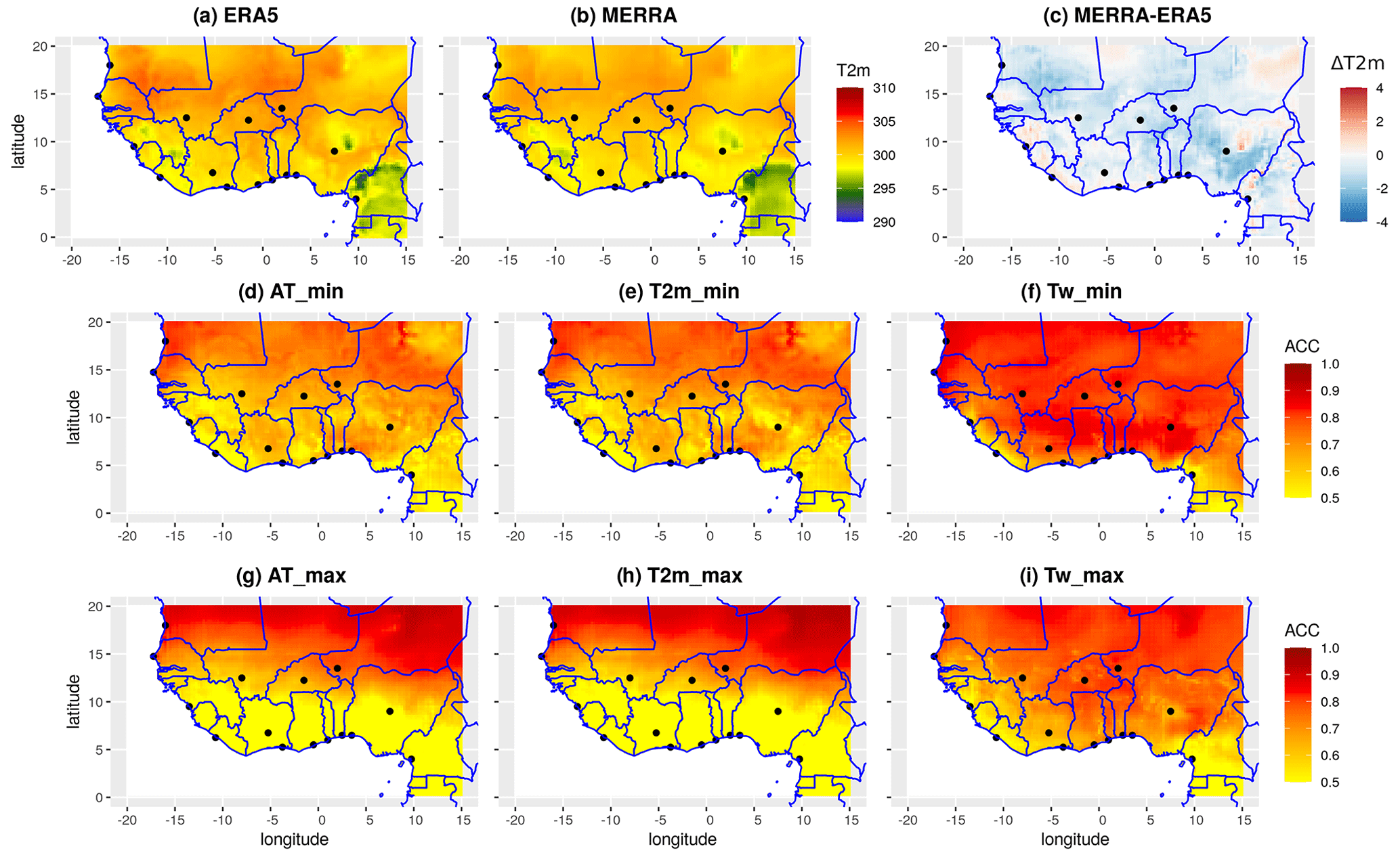
Figure 3Assessment of the evolution of some atmospheric variables in the reanalyses data: (a–b) climatology state of T2 m over 1993–2020 for ERA5 and MERRA respectively; (c) climatological bias between MERRA and ERA5 using ERA5 as reference (ΔT2 m); (d–f)/(g–i) anomaly of correlation between MERRA and ERA5 respectively for min/max values using AT, T2 m and Tw variables. The x and y axes represent the longitude and latitude in degrees respectively. The colour bars show the temperature (T2 m) in kelvins and the values of the anomaly of temperature (ACC) respectively. The black points in the map represent the cities of interest analysed in this work (see the “Region of interest” section for more details); this applies for all the maps in the paper.
3.2 Sensitivity of heat wave detection to threshold values
As discussed earlier in Sect 2.3.2, “Heat wave detection”, the threshold value used for heat wave monitoring has a significant impact on heat wave characteristics. The threshold value is generally tailored to the application that is to be carried out. In this part of the work, we investigate the sensitivity of heat wave frequency to different thresholds. To achieve this goal, we define four relative threshold values calculated over the entire period: the 75th, 80th, 85th and 90th daily percentiles. The choice of these thresholds for assessing changes in heat wave characteristics is based on previous work. Many studies use the 90th percentile to define a heat wave (e.g. Fischer and Schär, 2010; Perkins et al., 2012a; Déqué et al., 2017; Lavaysse et al., 2018; Barbier et al., 2018); other studies use the 75th percentile (Guigma et al., 2020). Based on these studies, we decided to test the sensitivity of threshold values from the third quartile (75th percentile) to the 90th percentile by steps of 5 % to quantify significant changes in heat wave frequency. As we are studying extreme events, it is not relevant to go below the third quartile; knowing also that this study focuses on human impacts of heat waves, the 90th percentile is enough as a maximum threshold. Heat wave detection is treated separately for these four thresholds (see Fig. S7). The sensitivity of heat wave frequency or duration with respect to the thresholds (75th, 80th, 85th, 90th percentiles) is treated independently for the four thresholds; this is done by calculating the linear evolution coefficient over each grid point. The linear evolution coefficient is defined as the slope of the linear regression line fitted between the threshold values (Q75, Q80, Q85, Q90) and the number of events associated with each threshold (NQ75, NQ80, NQ85, NQ90) or their corresponding duration (DQ75, DQ80, DQ85, DQ90). The calculation of the linear evolution coefficient is carried out according to the following steps:
-
After processing for heat wave detection at each grid point for the four thresholds separately, we compute for each of them the frequency and duration of heat waves.
-
Then we fit a regression line between the threshold values (Q75, Q80, Q85, Q90) and their corresponding frequency or duration. This is done for each grid point.
-
Finally, the changes in heat wave occurrence/duration from the 75th to 90th percentiles at each grid point are given by the computation of the slope of the regression line fitted at step 2 between the threshold values and their corresponding heat wave occurrence/duration.
We are aware that this regression based on four points is not very robust; nevertheless it makes it possible to obtain information on the evolution of the heat wave characteristics with respect to the thresholds. We therefore assessed the significance of the slope values with respect to the thresholds using a confidence level of 95 %. The significance of the slope was evaluated using a two-sided chi-squared statistics test (Pandis, 2016).
The linear evolution is given by the following equations:
where aw, and bw, are the slopes and intercepts of the regressions at the grid point w for heat wave frequency and duration respectively.
This analysis is conducted with T2 m and Tw extracted from MERRA and ERA5 reanalyses. We find a high spatial variability in the sensitivity of heat wave occurrence to the threshold values over West African regions (Figs. S8 and S9). Some regions are more sensitive than others; this can be explained by a strong seasonal cycle of the T2 m and Tw signals in those regions. We observe small changes in the frequency and duration of heat waves with respect to the thresholds when using the minimum and maximum values of T2 m or Tw (Figs. S8c, f, 4c, f and S9c, f); this is related to the small sample size of events detected with method 3 (see Sect. 2.3.2 for more details). As the results show, the frequency of heat waves can be expected to increase with decreasing threshold values (see Figs. S8 and S7). Heat waves detected using low threshold values are very persistent and last for several days (Fig. 4 shows an illustration with T2 m used as an indicator). This can be explained by the fact that when using a low threshold value, one can expect to have many days with temperature values above the daily threshold. Conversely, for heat waves detected with high threshold values, the duration of the events is considerably reduced. This is statistically coherent because the number of consecutive days with temperature above the threshold will decrease as the threshold increases. In general, we find that the duration of heat waves is more sensitive to the threshold values than their frequency. This is very coherent because the persistence of a heat wave will be mainly affected by the threshold values used for the detection.
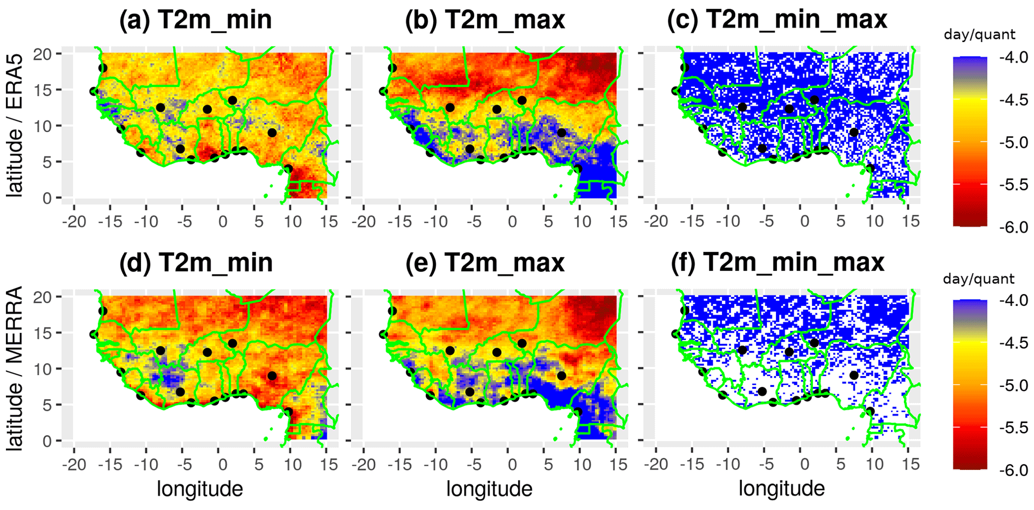
Figure 4Evolution of the heat wave duration with respect to the threshold values using T2 m as an indicator for (a–c) ERA5 and (d–f) MERRA respectively. The figure shows the slope of the regression line in days per percentile, which is computed by fitting a linear regression between the threshold values (Q75, Q80, Q85, Q90) and their corresponding heat waves's duration (DQ75, DQ80, DQ85, DQ90). The x and y axes represent the longitude and latitude in degrees respectively. The colour bar shows the values of the slope. The white blanks indicate non-significant changes in the duration of heat waves per percentile. The significance of the slope of the regression line has been computed using a two-sided chi-squared test.
3.3 Sensitivity of heat wave detection to the choice of indicators and methods applied
We have shown that the heat wave detection is very sensitive to threshold values. Based on the literature review and the application of this work, for the rest of the study, we use the 90th percentile for heat wave analyses (e.g. Fischer and Schär, 2010; Perkins et al., 2012a; Perkins and Alexander, 2013; Fontaine et al., 2013; McGregor et al., 2015; Russo et al., 2016; Mutiibwa et al., 2015; Oueslati et al., 2017; Déqué et al., 2017; Batté et al., 2018; Barbier et al., 2018; Lavaysse et al., 2018; Yu et al., 2021; Engdaw et al., 2022) using ERA5 reanalysis (Fig. 5). We identified four indicators – T2 m, Tw, AT and UTCI – from which heat wave detection was processed using three different methods (see Sect. 2.3 for more details). We notice that the occurrences of daytime and nighttime heat waves (Fig. 5a–d, e–h) are in the same range of values, while for concomitant events (Fig. 5i–l), the occurrence of heat waves is drastically reduced by . This could be explained by the facts that nighttime and daytime heat waves do not necessarily occur at the same time and their origins are totally different. Daytime heat waves will be mainly influenced by incoming solar radiation, while nighttime heat waves will be mainly influenced by the water vapour content of the air mass (Barbier et al., 2018; Largeron et al., 2020). We observe a high occurrence of nighttime heat waves over the coastal region from Guinea to Cameroon (Fig. 5a–d) linked to moist air coming from the Atlantic Ocean in the region during the night; daytime heat waves are more frequent in the Sahel and north-east of the Sahara (Fig. 5e–h) due to hot temperatures over the continental regions. When analysing nighttime heat wave events from each indicator (Fig. 5a–d), it appears that Tw heat waves are more frequent than T2 m/AT/UTCI events. It seems that Tw is more sensitive to humidity than the other indicators (see formula of Tw); this could explain the high frequency of events observed during the night in the coastal region. Regarding daytime heat waves (Fig. 5e–h), the spatial variability of events is more consistent for all the indicators in the Sahelian zone. However, some differences are observed: an increase in heat wave occurrence over the coastal region with Tw is noticed compared to T2 m, AT and UTCI. The detection of heat wave events with method 3 shows that Tw events are more frequent than T2 m/AT/UTCI events with a maximum of occurrence located over the northern Sahel. This means that daytime and nighttime heat waves occur frequently and simultaneously over the Sahel with Tw. From this result, we can deduce that humidity plays a major role in the occurrence of concomitant heat waves, which are very dangerous for human health. In this section, we show the high sensitivity of heat wave detection to the methodology applied and to the variables used as indicators. The role of humidity in heat wave occurrence in the coastal region has also been highlighted. Similar results are found with MERRA reanalysis (not shown).
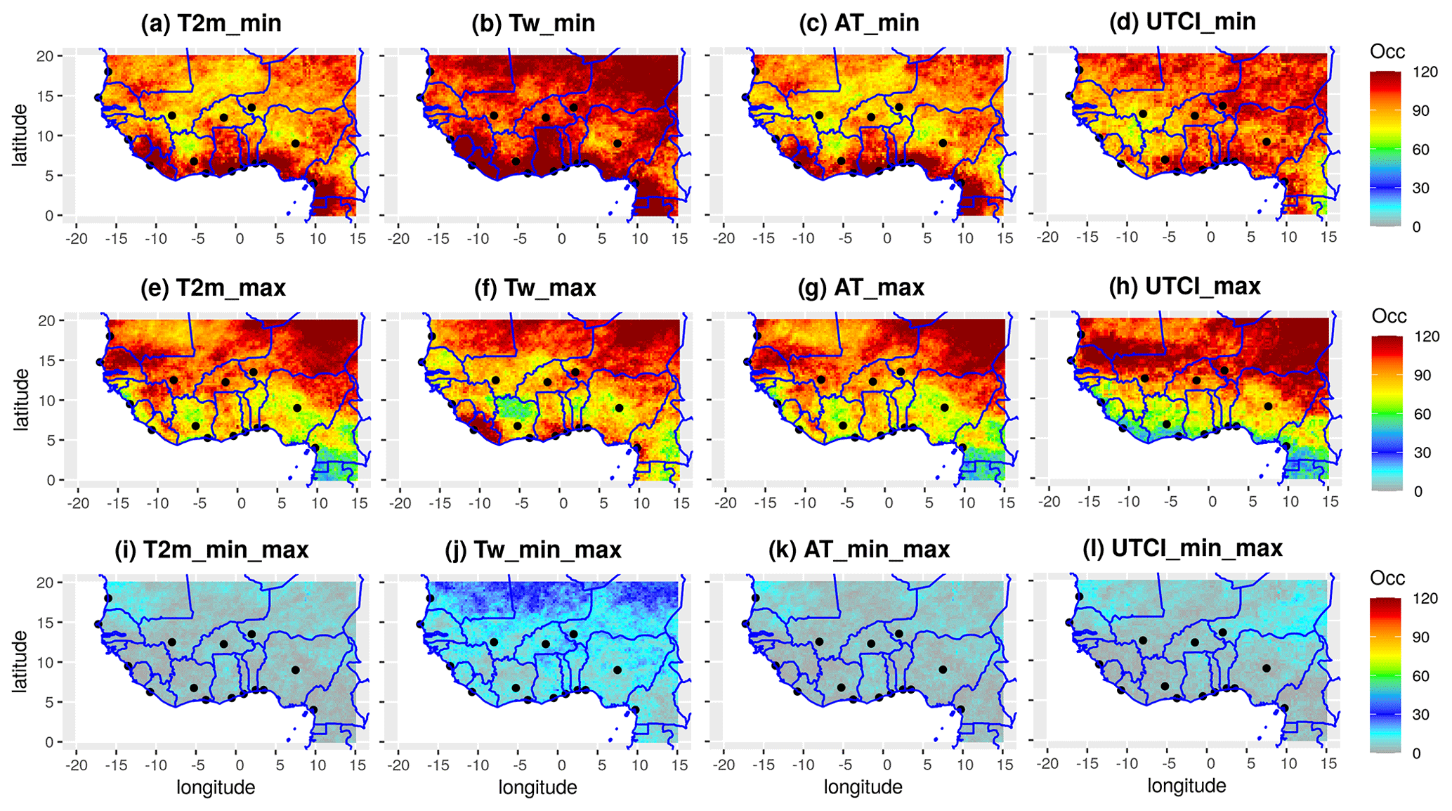
Figure 5Climatological state of heat wave occurrence over West Africa during the period 1993–2020 using four different indicators (T2 m, Tw, AT, UTCI). The detection of heat waves is based on the definition adopted: (a–d) minimum values of indicators, (e–h) maximum values of indicators, and (i–l) minimum and maximum values of indicators. The detection of heat waves was processed using ERA5 reanalysis and the climatological daily 90th percentile over the period as a threshold. The x and y axes represent the longitude and latitude in degrees respectively. The colour bar shows the frequency of heat waves per region.
In summary, the heat wave detection is influenced by many parameters: the dataset, threshold values, indicators and methodology used to define such an event. There is a high dependency between these parameters and the climatic region investigated. We illustrate the sensitivity of heat wave characteristics to the previous parameters in the CONT region (Fig. 6), as well as the ATL and GU regions (see Figs. S10 and S11) using ERA5 and MERRA reanalyses.
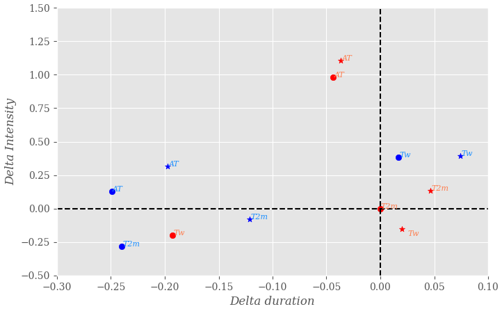
Figure 6Sensitivity analysis of heat wave characteristics to the datasets, indicators and methodologies used in the CONT region. The characteristics investigated here are the duration and intensity. The circles and stars in the figure represent ERA5 and MERRA reanalyses respectively. The blue/red colour represents minimum/maximum values of the indicators. “” from ERA5 is the reference variable used for this analysis. The x and y axes show the standardized variation in intensity and duration from the reference (no unit) respectively. The variations in duration and intensity have been computed using max daily T2 m in ERA5 as reference. The detection of heat waves is done using the climatological daily 90th percentile over the period as a threshold.
3.4 Monitoring of heat waves over West Africa regions
In this section, we analyse the spatial variability of heat waves in three climate regions (CONT, ATL and GU; see the “Region of interest” section for more details) using T2 m, AT and Tw as indicators and reanalysis data. Although ERA5 is slightly better than MERRA when compared to station data (Fig. S3b), we have evaluated the recent evolution of heat waves in both reanalyses. To do so, we firstly assessed the interannual variability of heat waves and their characteristics from 1993 to 2020. For each region, the characteristics of heat waves were calculated as the ratio of the sum of the characteristics of all the cities belonging to a region divided by the number of cities. We identified some particularly hot years with a high frequency of nighttime, daytime and concomitant heat waves: 1998, 2005, 2010, 2016, 2019 and 2020 in the three regions for all the indicators (see Figs. 7, S12 and S13). These peak heat wave years are addressed in Sect. 4. The GU region appears to have experienced more heat waves over the last decade than the CONT and ATL regions (see Fig. S12 for daytime events and Fig. S13 for nighttime). The mean duration of heat waves detected in the three regions is in the same range of values with some specific persistent events at the end of the period in the ATL and GU regions (not shown). Stronger and more persistent heat waves are found in the CONT region. From a statistical point of view, this is due to less variability in the signal of indicators in the region, which favours the detection of consecutive days with indicator values above the threshold. The highest occurrences of heat waves in the three regions are associated with Tw for daytime and nighttime events (see Figs. S12 and S13 respectively). Conversely, high-intensity heat waves are associated with AT (not shown) in the three regions. We can infer from this result that AT presents a more stable signal in the regions compared to T2 m and Tw. Concomitant high-intensity events are found in the CONT and ATL regions (see Fig. S15).

Figure 7Interannual variability of heat wave characteristics using maximum values of T2 m, Tw and AT for (a–c) duration and (d–f) intensity. The detection of heat waves is done using the climatological daily 90th percentile as a threshold over the period, and the characteristics of heat waves are computed in the three regions: (a, d) CONT, (b, e) ATL and (c, f) GU. The solid and dashed red/blue/green lines represent the evolution of heat wave characteristics using T2 m/Tw/AT from ERA5 and MERRA respectively. The x and y axes represent the duration and intensity of heat waves and the time in year respectively.
We also investigate the seasonal distribution of heat wave occurrence in the three regions. We find an increase in the frequency of daytime and nighttime heat waves at the beginning of the season and during the retreat period of the West Africa monsoon (starting in September; see Fig. S14a–c). A decrease in heat wave frequency is observed during the active phase of the monsoon in the three regions; this is consistent because the monsoon flow brings rainfall into the region, resulting in a cooling effect. The concomitant heat waves show a seasonal cycle with strong fluctuations (Fig. S16). This is due to the fact that concomitant events are conditioned by daytime and nighttime heat waves, which are two distinct processes.
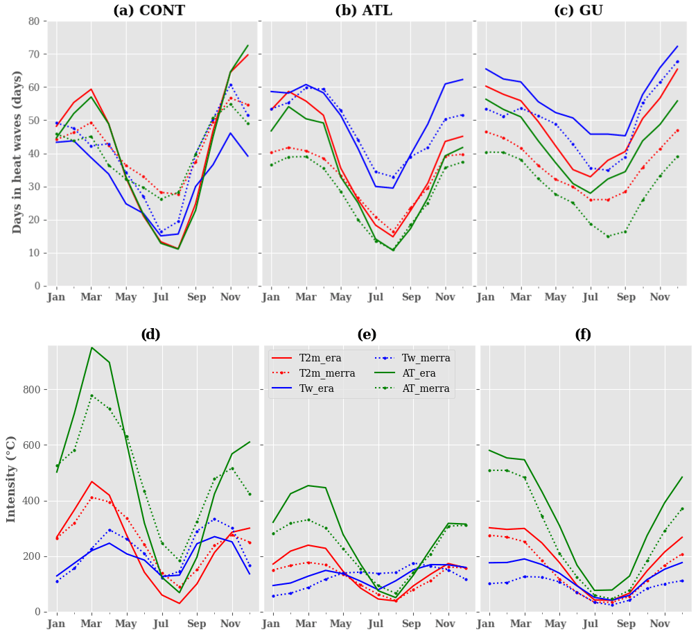
Figure 8Seasonal variability of heat wave characteristics using maximum values of T2 m, Tw and AT for (a–c) duration and (d–f) intensity respectively. We compute a 3-month running mean to smooth the seasonal cycle. The detection of heat waves is done using the climatological daily 90th percentile as a threshold in the different regions: (a–d) CONT, (b–e) ATL and (c–f) GU. The solid and dashed red/blue/green lines represent the evolution of heat wave characteristics using T2 m/Tw/AT from ERA5 and MERRA respectively. The y and x axes represent the duration and intensity of heat waves and the time in months respectively.
The seasonal cycle of the duration and intensity of heat waves follows the same distribution as the heat wave occurrence (see Fig. 8a–c and d–f respectively). Persistent and strong-intensity heat waves (nighttime, daytime) occur at the beginning and the end of the season, while short-duration and low-intensity events occur during the monsoon phase (Fig. 8a–c, d–f). This is verified for all the three indicators despite some discrepancies. The period 1993–2020 is then divided into 3 decades – 1993–2001, 2002–2011 and 2012–2020 – and we evaluate the contribution of each decade to the heat wave characteristics over the whole period (see Fig. 9 for heat wave duration). Results are similar when analysing the intensity of heat waves (not shown). The percentiles used for the detection of heat waves in each decade are computed over the whole period 1993–2020. It is clearly shown with ERA5 that the major contribution to heat wave characteristics over the period comes from the last decade (Fig. 9g–i). We notice a progressive increase in frequency, duration and intensity of all the heat waves (daytime, nighttime and concomitant) from the first to the last decade in the three regions (see Figs. S14j–l and S16j–l); this is true for all the indicators. Using ERA5 reanalysis, we found the last decade (2012–2020) shows a major contribution to around 50 % of heat wave characteristics over the period 1993–2010, while the first and second decades contribute up to 22.4 % and 27.6 % respectively. This contribution of the last decade over the total period is not effective in MERRA reanalysis, where the different decades appear to have a similar contribution. This is the result of the uncertainties highlighted earlier in both reanalyses. The reinforcement of extreme events such as heat waves during the last decade in ERA5 is possibly linked to global warming. This result is consistent with other studies that show an increase in heat wave frequency and characteristics under climate change (e.g. Dosio, 2017; Dosio et al., 2018; Murari and Ghosh, 2019; Lorenzo et al., 2021; Engdaw et al., 2022). When analysing the severity of heat waves over the previous 3 decades using the mean duration and intensity (see Fig. S17 and S18), we do not find a significant increase in heat wave characteristics.
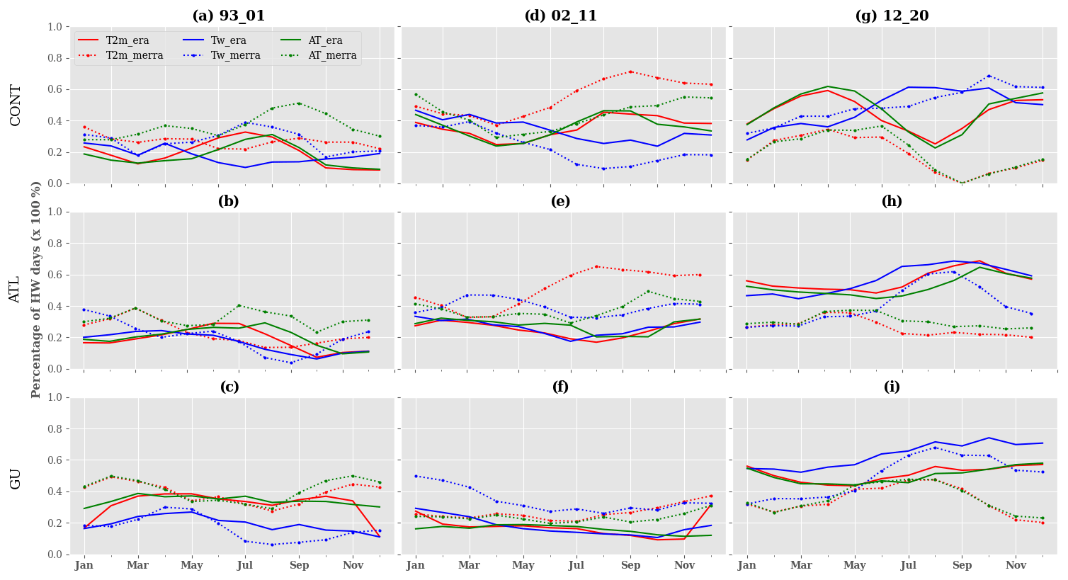
Figure 9Contribution in percent of the different decades to heat wave duration using maximum values of T2 m, Tw and AT over the whole period for (a–c) 1993–2001, (d–f) 2002–2011 and (g–i) 2012–2020. We compute a 3-month running mean to smooth the seasonal cycle. The detection of heat waves is done using the 90th percentile as a threshold over the period in the different regions: (a, d, g) CONT, (b, e, h) ATL and (c, f, i) GU. The solid and dashed red/blue/green lines represent the evolution of heat wave duration using T2 m/Tw/AT from ERA5 and MERRA respectively. The y and x axes represent the percentage of heat wave days and the time in months respectively.
After the evaluation of the temporal evolution of heat waves over the three regions, we analyse their persistence based on their duration using ERA5 and MERRA reanalyses and maximum values of the indicators (see Figs. 10 and S19 respectively). We defined five types of event as described in Table 3. We observed that approximately 75 % of daytime heat waves have a duration of 3–6 d with at least 40 % of events belonging to C1 (Fig. 10). Very persistent daytime heat waves contribute to at least 9 %–13 % of the events registered. Severe and very severe daytime events are extremely rare in the region, and they contribute up to 12 % of the total number of heat waves. The classification is not too sensitive to indicators and regions. We obtained a similar classification with nighttime heat waves (not shown).
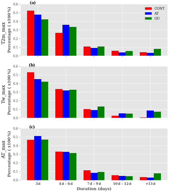
Figure 10Classification of heat waves using ERA5 reanalysis based on their persistence over the period 1993–2020: (a) T2 m, (b) Tw and (c) AT. The detection of heat waves is done using maximum values of the indicators and the climatological daily 90th percentile. Heat wave detection is firstly carried out, and then their duration is computed. Clusters of heat waves based on their duration (3, 4–6, 7–9, 10–12, 13+ d) are created, and finally, we quantify each class of heat waves as a proportion of the total number of events detected. The y and x axes represent the percentage of the heat waves per class and the duration in days respectively. The red/blue/green bars represent the percentage of heat waves detected over CONT/ATL/GU regions (see the “Region of interest” section for more details). The sum of the contribution of heat waves in different clusters is equal to 1 for each region.

We analyse the evolution of heat wave occurrence and characteristics over a variety of climatic regions in West Africa. The spatial variability of heat wave indicators (T2 m and Tw) over West Africa during the seasons (winter, spring, summer and autumn) was investigated. This is done through the computation of the interannual daily standard deviation over the period 1993–2020. We find the lowest values of standard deviation over the three regions of interest (CONT, ATL and GU) during the summer and autumn when we use minimum values of T2 m () (see Fig. S20). This shows low variability in the signal of , which indicates favourable conditions for the occurrence of persistent heat waves in these regions during this period. With Tw, there is low variability in the signal during the summer for both minimum and maximum values, indicating persistent events. We find some discrepancies in the reanalysis products ERA5 and MERRA. The results show that ERA5 appears to be hotter than MERRA over the Sahel region. The source of these discrepancies in the reanalyses is very complex and may result from different factors such as the data assimilation techniques (4D-Var and Bonavita et al., 2016, for ERA5; 3D-Var and Courtier et al., 1998, for MERRA), atmospheric models, convective schemes, bias correction methods, spatial resolution and model parameterization. Another major difference between ERA5 and MERRA is in the vertical resolution of the profiles of the atmospheric variables between 0 and 2 km; ERA5 has more atmospheric vertical levels than MERRA below 2 km, which leads to a more accurate representation of processes in the boundary layer (Taszarek et al., 2021). Many studies have highlighted these differences in the two reanalysis products (e.g. Olauson, 2018; Graham et al., 2019; Taszarek et al., 2021); some authors (e.g. Gensini et al., 2014; Tippett et al., 2014; Allen et al., 2015; Taszarek et al., 2018; King and Kennedy, 2019) have identified model parameterization and the data assimilation technique as possible causes of biases in reanalyses for low-level thermodynamic fields. A more detailed study of the source of these uncertainties is beyond the scope of this paper.
An assessment of the origins of heat waves in the coastal regions of West Africa is discussed. One driver of heat waves over the globe highlighted by many studies is the “blocking high” (e.g. Charney and DeVore, 1979; Coughlan, 1983; Perkins, 2015). This situation occurs when a high system pressure remains in the same region for a longer period of time than is usually expected. The consequence of this phenomenon is the compression of the air mass at the surface, which leads to an increase in temperatures in the region. Perkins (2015) also identified soil moisture–atmosphere interactions and large-scale climate dynamics as other drivers of heat waves.
To address the origin of heat waves in the coastal region, we firstly analysed the interannual variability in the sea surface temperature (SST) over the period 1993–2020 using the ERA5 reanalysis. We computed the mean anomalies of SST with respect to the climatology (Fig. S21). Warming over the north-eastern and south-eastern tropical Atlantic Ocean is observed in some years: 1998, 2005, 2008, 2010, 2016, 2019 and 2020. This warming over the tropical Atlantic Ocean affects the whole western African coastal region. In comparison to the interannual variability of heat wave occurrence in the coastal region (see Fig. S12), we noticed that the years of high heat wave frequency correspond to years in which ocean warming was observed: 1998, 2005, 2010, 2016, 2019 and 2020 for instance. These years also correspond to the occurrence of El Niño events. The link between the SST and heat waves has been investigated in more detail in the following. We computed the yearly mean SST anomalies with respect to heat waves days using the formula below:
where αi represents the total number of days in heat waves per month for each year; if there is no event detected, then αi=0.
For this analysis, we focused on the years with high peaks of heat waves identified previously (1998, 2005, 2008, 2010, 2016, 2019 and 2020) using T2 m as an indicator for heat wave detection. We noticed that most of the heat waves are associated with a warming of the tropical Atlantic Ocean except for in some specific years such as 2016 and 2019 in the GU and ATL regions respectively (Fig. 11a, b). In the CONT region, heat waves are influenced by both the west–east airflow coming from the tropical northern Atlantic Ocean and the south–north airflow coming from the tropical southern Atlantic Ocean (Fig. 11c, d). Some years in which a considerable number of heat waves have been detected are not associated with positive anomalies of SST. These heat waves occur during a cold phase of the tropical Atlantic Ocean. There are no major changes observed in the analysis when using AT and Tw as indicators for heat wave detection (not shown). We can suggest from this result that heat waves in the coastal region have many drivers, and one of them at a local scale could be the oceanic forcings through the SST. Large-scale (El Niño, atmospheric circulation) and local-scale (soil–moisture interactions) processes may also contribute to the occurrence of heat waves in the region. This result is in agreement with Russo et al. (2016) and Moron et al. (2016), who identified links between heat waves and El Niño events. The investigation of the physical processes driving heat waves in the coastal region required more in-depth knowledge of local- and large-scale forcings, which is beyond the scope of this paper.
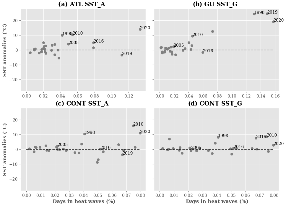
Figure 11Analysis of the link between SST anomalies and heat waves days over the period 1993–2020 using ERA5 reanalysis and maximum values of T2 m in the different regions: (a) ATL, (b) GU, (c–d) CONT. SST_A and SST_G represent the boxes using to compute the SST mean anomalies for the ATL and CONT regions respectively (see Fig. 1). The anomalies are computed as the difference between monthly SST and the monthly climatological values of the SST over the whole period. For each year, the yearly anomalies of SST are computed with respect to the heat waves days. The x and y axes represent the frequency of heat waves days and the SST anomalies respectively. The grey dots represent the years over the period 1993–2020.
The present work assesses the potential uncertainties associated with heat wave detection using reanalysis data (ERA5, MERRA). It also looks into the recent evolution of heat waves in different parts of the West African region.
The first uncertainty highlighted in this study comes from the ERA5 and MERRA reanalyses. We found biases in the reanalysis products; MERRA shows a cold bias compared to ERA5 over the Sahel region and the Guinean region except over some countries (Guinea-Bissau, Sierra Leone, Liberia). Weak correlations between ERA5 and MERRA were found over the Guinea coast using minimum/maximum values of T2 m and AT indicators. The representation of extreme values in the reanalyses was analysed, showing that the coherence between the two products is very low, around 0.25, in the southern Sahel and the Guinean region. This low agreement between the two reanalyses results in discrepancies in the frequency of heat waves associated with each product. Even though the reanalyses present large discrepancies over the southern Sahel and Guinea coast, they are able to preserve the relationship between the variables used for heat wave detection (AT, T2 m). Temperatures estimated from local station in Dakar and Abidjan show slightly better correlation with ERA5 than with MERRA. The second uncertainty found here is the sensitivity of the spatial variability of heat waves to the threshold values used to process the monitoring of events. Heat waves detected using low threshold values of the indicators T2 m and Tw are very persistent and last for several days, while the duration of heat waves related to the high threshold values is considerably reduced. We notice some discrepancies in the sensitivity to the threshold values of heat waves detected with Tw and T2 m. Nighttime and daytime heat waves are in the same range of occurrence, while concomitant events are extremely rare because they are more restrictive. This shows that daytime and nighttime heat waves are distinct phenomena. The climatological state of heat wave occurrence shows large differences between the indicators. Nighttime heat waves associated with Tw are more frequent than those detected with AT, T2 m and UTCI. This shows that humidity plays an important role in nighttime events and tends to reinforce concomitant events over the northern Sahel. The spatial variability of daytime heat waves is more consistent for all indicators over the Sahel. The interannual variability of heat waves in the coastal region of West Africa shows for the three indicators (AT, T2 m, Tw) some particularly hot years with a high frequency of events: 1998, 2005, 2010, 2016, 2019 and 2020 linked to El Niño events. The GU region is more affected by heat waves during the last decade (2012–2020) than the CONT and ATL regions. The CONT region experienced more persistent and higher-intensity heat waves than the GU region. The seasonal cycle of heat waves shows an increase in the frequency of the events at the beginning of the season and during the retreat phase of the West African monsoon. Conversely, a decrease in heat wave occurrence is observed during the monsoon activity period in the three regions. We observed a reinforcement in the frequency, duration and intensity of heat waves during the last decade (2012–2020). This is a consequence of global warming acting on extreme events. No significant changes in the severity of heat waves have been found in the regions during the 3 decades. Most of the events detected in the regions (75 %) have a duration of around 3–6 d. The most dangerous events, lasting at least 10 d, accounted for up to 12 % of the total number of events. We noticed strong links between SST and heat waves during some specific peak event years, but this was not the case for 2016 and 2019 in the GU and ATL regions respectively. We can infer from this result that there is a contribution of oceanic forcings in the reinforcement of heat waves in the coastal region among many other drivers. In a future work, we will investigate in more detail the influence of large-scale forcings on heat wave occurrence in this region. In the present study, we detected different types of heat wave based on the methodology and indicator used; this will be very important to investigate their potential impacts on human health and activities.
The codes to perform heat wave detection, data interpolation and the rest of the analyses are available on request; please feel free to contact us. The codes were implemented using CDO, R (heatwaveR) and Python libraries.
The data used in this study are mostly open access. Data from the ERA5 and MERRA reanalyses are available online at the Climate Data Store (CDS: https://doi.org/10.24381/cds.adbb2d47, Hersbach et al., 2023) and on the NASA (https://doi.org/10.5067/VJAFPLI1CSIV, GMAO, 2015) website respectively. Local station data are not freely available; feel free to write to us if you need them.
The supplement related to this article is available online at: https://doi.org/10.5194/nhess-23-1313-2023-supplement.
This study was conducted with the collaboration of different researchers, who played an important role at each step. CGNL performed the analyses and the interpretation of the results; CL supervised the work and made some good remarks; MV brought his expertise in statistical interpolation. CGNL, CL, CF and MV discussed the results and wrote the paper. CF and MV provided advice and insightful comments before submission.
The contact author has declared that none of the authors has any competing interests.
Publisher's note: Copernicus Publications remains neutral with regard to jurisdictional claims in published maps and institutional affiliations.
This work is supported by the French National Research Agency in the framework of the STEWARd project under grant ANR-19-CE03-0012 (2020–2024).
This research has been supported by the Agence Nationale de la Recherche (STEWARd; grant no. ANR-19-CE03-0012).
This paper was edited by Maria-Carmen Llasat and reviewed by two anonymous referees.
Alduchov, O. A. and Eskridge, R. E.: Improved Magnus form approximation of saturation vapor pressure, J. Appl. Meteorol. Clim., 35, 601–609, 1996. a, b
Allen, J. T., Tippett, M. K., and Sobel, A. H.: An empirical model relating US monthly hail occurrence to large-scale meteorological environment, J. Adv. Model. Earth Sy., 7, 226–243, 2015. a
Anderson, B. G. and Bell, M. L.: Weather-Related Mortality, Epidemiology, 20, 205–213, https://doi.org/10.1097/EDE.0b013e318190ee08, 2009. a
August, E. F.: Ueber die Berechnung der Expansivkraft des Wasserdunstes, Ann. Phys., 89, 122–137, https://doi.org/10.1002/andp.18280890511, 1828. a
Barbier, J., Guichard, F., Bouniol, D., Couvreux, F., and Roehrig, R.: Detection of Intraseasonal Large-Scale Heat Waves: Characteristics and Historical Trends during the Sahelian Spring, J. Climate, 31, 61–80, https://doi.org/10.1175/JCLI-D-17-0244.1, 2018. a, b, c, d, e, f, g, h
Batté, L., Ardilouze, C., and Déqué, M.: Forecasting West African Heat Waves at Subseasonal and Seasonal Time Scales, Mon. Weather Rev., 146, 889–907, https://doi.org/10.1175/MWR-D-17-0211.1, 2018. a, b
Beniston, M., Stoffel, M., and Guillet, S.: Comparing observed and hypothetical climates as a means of communicating to the public and policymakers: The case of European heatwaves, Environ. Sci. Policy, 67, 27–34, https://doi.org/10.1016/j.envsci.2016.11.008, 2017. a
Bonavita, M., Hólm, E., Isaksen, L., and Fisher, M.: The evolution of the ECMWF hybrid data assimilation system, Q. J. Roy. Meteor. Soc., 142, 287–303, https://doi.org/10.1002/qj.2652, 2016. a
Braga, A. L. F., Zanobetti, A., and Schwartz, J.: The effect of weather on respiratory and cardiovascular deaths in 12 U.S. cities, Environ. Health Persp., 110, 859–863, https://doi.org/10.1289/ehp.02110859, 2002. a
Buck, A. L.: New equations for computing vapor pressure and enhancement factor, J. Appl. Meteorol. Clim., 20, 1527–1532, 1981. a
Ceccherini, G., Russo, S., Ameztoy, I., Marchese, A. F., and Carmona-Moreno, C.: Heat waves in Africa 1981–2015, observations and reanalysis, Nat. Hazards Earth Syst. Sci., 17, 115–125, https://doi.org/10.5194/nhess-17-115-2017, 2017. a, b
Charney, J. G. and DeVore, J. G.: Multiple flow equilibria in the atmosphere and blocking, J. Atmos. Sci., 36, 1205–1216, 1979. a
Coughlan, M.: A comparative climatology of blocking action in the two hemispheres, Aust. Meteorol. Mag., 31, 3–13, 1983. a
Courtier, P., Andersson, E., Heckley, W., Vasiljevic, D., Hamrud, M., Hollingsworth, A., Rabier, F., Fisher, M., and Pailleux, J.: The ECMWF implementation of three-dimensional variational assimilation (3D-Var). I: Formulation, Q. J. Roy. Meteor. Soc., 124, 1783–1807, https://doi.org/10.1002/qj.49712455002, 1998. a
Déqué, M., Calmanti, S., Christensen, O. B., Aquila, A. D., Maule, C. F., Haensler, A., Nikulin, G., and Teichmann, C.: A multi-model climate response over tropical Africa at +2 ∘C, Climate Services, 7, 87–95, 2017. a, b, c
Di Napoli, C., Barnard, C., Prudhomme, C., Cloke, H. L., and Pappenberger, F.: ERA5-HEAT: A global gridded historical dataset of human thermal comfort indices from climate reanalysis, Geosci. Data J., 8, 2–10, https://doi.org/10.1002/gdj3.102, 2021. a
Dosio, A.: Projection of temperature and heat waves for Africa with an ensemble of CORDEX Regional Climate Models, Clim. Dynam., 49, 493–519, https://doi.org/10.1007/s00382-016-3355-5, 2017. a
Dosio, A., Mentaschi, L., Fischer, E. M., and Wyser, K.: Extreme heat waves under 1.5 ∘C and 2 ∘C global warming, Environ. Res. Lett., 13, 054006, https://doi.org/10.1088/1748-9326/aab827, 2018. a
Engdaw, M. M., Ballinger, A. P., Hegerl, G. C., and Steiner, A. K.: Changes in temperature and heat waves over Africa using observational and reanalysis data sets, Int. J. Climatol., 42, 1165–1180, 2022. a, b, c, d, e, f, g, h
Eyring, V., Gillett, N. P., Achutarao, K., Barimalala, R., Barreiro Parrillo, M., Bellouin, N., Cassou, C., Durack, P., Kosaka, Y., McGregor, S., Min, S., Morgenstern, O., and Sun, Y.: Human Influence on the Climate System, in: Climate Change 2021: The Physical Science Basis. Contribution of Working Group I to the Sixth Assessment Report of the Intergovernmental Panel on Climate Change, IPCC Sixth Assessment Report, edited by: Masson-Delmotte, V., Zhai, V., Pirani, A., Conners, S. L., Péan, C., Berger, S., Caud, N., Chen, Y., Goldfarb, L., Gomis, M. I., Huang, M., Leitzell, K., Lonnoy, E., Matthews, J. B. R., Maycock, T. K., Waterfield, T., Yelekçi, O., Yu, R., and Zhou, B., Cambridge University Press, https://elib.dlr.de/144265/ (last access: 4 April 2023), 2021. a
Fischer, E. M. and Schär, C.: Consistent geographical patterns of changes in high-impact European heatwaves, Nat. Geosci., 3, 398–403, 2010. a, b, c, d
Fontaine, B., Janicot, S., and Monerie, P.-A.: Recent changes in air temperature, heat waves occurrences, and atmospheric circulation in Northern Africa, J. Geophys. Res.-Atmos., 118, 8536–8552, https://doi.org/10.1002/jgrd.50667, 2013. a, b
Fouillet, A., Rey, G., Laurent, F., Pavillon, G., Bellec, S., Guihenneuc-Jouyaux, C., Clavel, J., Jougla, E., and Hémon, D.: Excess mortality related to the August 2003 heat wave in France, Int. Arch. Occ. Env. Hea., 80, 16–24, https://doi.org/10.1007/s00420-006-0089-4, 2006. a
Gasparrini, A. and Armstrong, B.: The impact of heat waves on mortality, Epidemiology, 22, 68–73, https://doi.org/10.1097/EDE.0b013e3181fdcd99, 2011. a, b
Gelaro, R., McCarty, W., Suárez, M. J., Todling, R., Molod, A., Takacs, L., Randles, C. A., Darmenov, A., Bosilovich, M. G., Reichle, R., Wargan, K., Coy, L., Cullather, R., Draper, C., Akella, S., Buchard, V., Conaty, A., da Silva, A. M., Gu, W., Kim, G.-K., Koster, R., Lucchesi, R., Merkova, D., Nielsen, J. E., Partyka, G., Pawson, S., Putman, W., Rienecker, M., Schubert, S. D., Sienkiewicz, M., and Zhao, B.: The Modern-Era Retrospective Analysis for Research and Applications, Version 2 (MERRA-2), J. Climate, 30, 5419–5454, https://doi.org/10.1175/JCLI-D-16-0758.1, 2017. a
Gensini, V. A., Mote, T. L., and Brooks, H. E.: Severe-thunderstorm reanalysis environments and collocated radiosonde observations, J. Appl. Meteorol. Clim., 53, 742–751, 2014. a
Gleixner, S., Demissie, T., and Diro, G. T.: Did ERA5 improve temperature and precipitation reanalysis over East Africa?, Atmosphere, 11, 996, https://doi.org/10.3390/atmos11090996, 2020. a
Global Modeling and Assimilation Office (GMAO): MERRA-2 tavg1_2d_slv_Nx: 2d,1-Hourly,Time-Averaged,Single-Level,Assimilation,Single-Level Diagnostics V5.12.4, Greenbelt, MD, USA, Goddard Earth Sciences Data and Information Services Center (GES DISC) [data set], https://doi.org/10.5067/VJAFPLI1CSIV, 2015. a
Graham, R. M., Hudson, S. R., and Maturilli, M.: Improved performance of ERA5 in Arctic gateway relative to four global atmospheric reanalyses, Geophys. Res. Lett., 46, 6138–6147, 2019. a
Guigma, K. H., Todd, M., and Wang, Y.: Characteristics and thermodynamics of Sahelian heatwaves analysed using various thermal indices, Clim. Dynam., 55, 3151–3175, https://doi.org/10.1007/s00382-020-05438-5, 2020. a, b, c, d
Hajat, S., Kovats, R. S., and Lachowycz, K.: Heat-related and cold-related deaths in England and Wales: who is at risk?, Occup. Environ. Med., 64, 93–100, https://doi.org/10.1136/oem.2006.029017, 2007. a
Hartmann, D. L., Tank, A. M. K., Rusticucci, M., Alexander, L. V., Brönnimann, S., Charabi, Y. A. R., Dentener, F. J., Dlugokencky, E. J., Easterling, D. R., Kaplan, A., Soden, B. J., Thorne, P. W., Wild, M., and Zhai, P. M.: Observations: atmosphere and surface, in: Climate change 2013 the physical science basis: Working group I contribution to the fifth assessment report of the intergovernmental panel on climate change, edited by: Stocker, T. F., Qin, D., Plattner, G.-K., Tignor, M., Allen, S. K., Boschung, J., Nauels, A., Xia, Y., Bex, V., and Midgley, P. M., Cambridge University Press, 159–254, 2013. a
Hersbach, H., Bell, B., Berrisford, P., Hirahara, S., Horányi, A., Muñoz-Sabater, J., Nicolas, J., Peubey, C., Radu, R., Schepers, D., Simmons, A., Soci, C., Abdalla, S., Abellan, X., Balsamo, G., Bechtold, P., Biavati, G., Bidlot, J., Bonavita, M., De Chiara, G., Dahlgren, P., Dee, D., Diamantakis, M., Dragani, R., Flemming, J., Forbes, R., Fuentes, M., Geer, A., Haimberger, L., Healy, S., Hogan, R. J., Hólm, E., Janisková, M., Keeley, S., Laloyaux, P., Lopez, P., Lupu, C., Radnoti, G., de Rosnay, P., Rozum, I., Vamborg, F., Villaume, S., and Thépaut, J.-N.: The ERA5 global reanalysis, Q. J. Roy. Meteor. Soc., 146, 1999–2049, https://doi.org/10.1002/qj.3803, 2020. a
Hersbach, H., Bell, B., Berrisford, P., Biavati, G., Horányi, A., Muñoz Sabater, J., Nicolas, J., Peubey, C., Radu, R., Rozum, I., Schepers, D., Simmons, A., Soci, C., Dee, D., and Thépaut, J.-N.: ERA5 hourly data on single levels from 1940 to present, Copernicus Climate Change Service (C3S) Climate Data Store (CDS) [data set], https://doi.org/10.24381/cds.adbb2d47, 2023. a
Huynen, M. M., Martens, P., Schram, D., Weijenberg, M. P., and Kunst, A. E.: The impact of heat waves and cold spells on mortality rates in the Dutch population, Environ. Health Persp., 109, 463–470, https://doi.org/10.1289/ehp.01109463, 2001. a
King, A. T. and Kennedy, A. D.: North American supercell environments in atmospheric reanalyses and RUC-2, J. Appl. Meteorol. Clim., 58, 71–92, 2019. a
Kovats, R. S. and Hajat, S.: Heat Stress and Public Health: A Critical Review, Annu. Rev. Publ. Health, 29, 41–55, https://doi.org/10.1146/annurev.publhealth.29.020907.090843, 2008. a
Largeron, Y., Guichard, F., Roehrig, R., Couvreux, F., and Barbier, J.: The April 2010 North African heatwave: when the water vapor greenhouse effect drives nighttime temperatures, Clim. Dynam., 54, 3879–3905, https://doi.org/10.1007/s00382-020-05204-7, 2020. a, b, c
Lavaysse, C., Cammalleri, C., Dosio, A., van der Schrier, G., Toreti, A., and Vogt, J.: Towards a monitoring system of temperature extremes in Europe, Nat. Hazards Earth Syst. Sci., 18, 91–104, https://doi.org/10.5194/nhess-18-91-2018, 2018. a, b, c, d, e
Lorenzo, N., Díaz-Poso, A., and Royé, D.: Heatwave intensity on the Iberian Peninsula: Future climate projections, Atmos. Res., 258, 105655, https://doi.org/10.1016/j.atmosres.2021.105655, 2021. a
Loughnan, M.: Heatwaves are silent killers, Geodate, 27, 7–10, 2014. a
Magnus, G.: Versuche über die Spannkräfte des Wasserdampfs, Annalen der Physik, 137, 225–247, https://doi.org/10.1002/andp.18441370202, 1844. a
McGregor, G. R., Bessmoulin, P., Ebi, K., and Menne, B.: Heatwaves and health: guidance on warning-system development, WMO and WHO, WMO-No. 1142, 114 pp., ISBN 978-92-63-11142-5, 2015. a, b, c, d
Moron, V., Oueslati, B., Pohl, B., Rome, S., and Janicot, S.: Trends of mean temperatures and warm extremes in northern tropical Africa (1961–2014) from observed and PPCA-reconstructed time series, J. Geophys. Res.-Atmos., 121, 5298–5319, 2016. a, b, c, d, e, f, g
Murari, K. K. and Ghosh, S.: Future Heat Wave Projections and Impacts, in: Climate Change Signals and Response: A Strategic Knowledge Compendium for India, edited by: Venkataraman, C., Mishra, T., Ghosh, S., and Karmakar, S., Springer, 91–107, https://doi.org/10.1007/978-981-13-0280-0_6, 2019. a
Mutiibwa, D., Vavrus, S. J., McAfee, S. A., and Albright, T. P.: Recent spatiotemporal patterns in temperature extremes across conterminous United States, J. Geophys. Res.-Atmos., 120, 7378–7392, 2015. a
Ngoungue Langue, C. G., Lavaysse, C., Vrac, M., Peyrillé, P., and Flamant, C.: Seasonal forecasts of the Saharan heat low characteristics: a multi-model assessment, Weather Clim. Dynam., 2, 893–912, https://doi.org/10.5194/wcd-2-893-2021, 2021. a, b
Olauson, J.: ERA5: The new champion of wind power modelling?, Renew. Energ., 126, 322–331, 2018. a, b
Oueslati, B., Pohl, B., Moron, V., Rome, S., and Janicot, S.: Characterization of Heat Waves in the Sahel and Associated Physical Mechanisms, J. Climate, 30, 3095–3115, https://doi.org/10.1175/JCLI-D-16-0432.1, 2017. a, b
Pandis, N.: The chi-square test, Am. J. Orthod. Dentofac., 150, 898–899, 2016. a
Perkins, S. E.: A review on the scientific understanding of heatwaves—Their measurement, driving mechanisms, and changes at the global scale, Atmos. Res., 164–165, 242–267, https://doi.org/10.1016/j.atmosres.2015.05.014, 2015. a, b, c, d
Perkins, S. E. and Alexander, L. V.: On the Measurement of Heat Waves, J. Climate, 26, 4500–4517, https://doi.org/10.1175/JCLI-D-12-00383.1, 2013. a, b, c
Perkins, S. E., Alexander, L. V., and Nairn, J. R.: Increasing frequency, intensity and duration of observed global heatwaves and warm spells, Geophys. Res. Lett., 39, L20714, https://doi.org/10.1029/2012GL053361, 2012. a, b, c
Ramon, J., Lledó, L., Torralba, V., Soret, A., and Doblas-Reyes, F. J.: What global reanalysis best represents near-surface winds?, Q. J. Roy. Meteor. Society, 145, 3236–3251, 2019. a
Robinson, P. J.: On the Definition of a Heat Wave, J. Appl. Meteorol. Clim., 40, 762–775, https://doi.org/10.1175/1520-0450(2001)040<0762:OTDOAH>2.0.CO;2, 2001. a
Rocklöv, J., Forsberg, B., Ebi, K., and Bellander, T.: Susceptibility to mortality related to temperature and heat and cold wave duration in the population of Stockholm County, Sweden, Global Health Action, 7, 22737, https://doi.org/10.3402/gha.v7.22737, 2014. a
Russo, S., Marchese, A. F., Sillmann, J., and Immé, G.: When will unusual heat waves become normal in a warming Africa?, Environ. Res. Lett., 11, 054016, https://doi.org/10.1088/1748-9326/11/5/054016, 2016. a, b, c
Shafiei Shiva, J., Chandler, D. G., and Kunkel, K. E.: Localized Changes in Heat Wave Properties Across the United States, Earth's Future, 7, 300–319, https://doi.org/10.1029/2018EF001085, 2019. a
Shaposhnikov, D., Revich, B., Bellander, T., Bedada, G. B., Bottai, M., Kharkova, T., Kvasha, E., Lezina, E., Lind, T., Semutnikova, E., and Pershagen, G.: Mortality Related to Air Pollution with the Moscow Heat Wave and Wildfire of 2010, Epidemiology, 25, 359–364, https://doi.org/10.1097/EDE.0000000000000090, 2014. a
Smith, T. T., Zaitchik, B. F., and Gohlke, J. M.: Heat waves in the United States: definitions, patterns and trends, Climatic Change, 118, 811–825, https://doi.org/10.1007/s10584-012-0659-2, 2013. a
Steadman, R. G.: The Assessment of Sultriness. Part I: A Temperature-Humidity Index Based on Human Physiology and Clothing Science, J. Appl. Meteorol. Clim., 18, 861–873, https://doi.org/10.1175/1520-0450(1979)018<0861:TAOSPI>2.0.CO;2, 1979a. a, b
Steadman, R. G.: The assessment of sultriness. Part II: effects of wind, extra radiation and barometric pressure on apparent temperature, J. Appl. Meteorol., 18, 874–885, 1979b. a, b
Steadman, R. G.: A universal scale of apparent temperature, J. Appl. Meteorol. Clim., 23, 1674–1687, 1984. a
Stefanon, M., D'Andrea, F., and Drobinski, P.: Heatwave classification over Europe and the Mediterranean region, Environ. Res. Lett., 7, 014023, https://doi.org/10.1088/1748-9326/7/1/014023, 2012. a
Stull, R.: Wet-Bulb Temperature from Relative Humidity and Air Temperature, J. Appl. Meteorol. Clim., 50, 2267–2269, https://doi.org/10.1175/JAMC-D-11-0143.1, 2011. a
Tan, J., Zheng, Y., Tang, X., Guo, C., Li, L., Song, G., Zhen, X., Yuan, D., Kalkstein, A. J., Li, F., and Chen, H.: The urban heat island and its impact on heat waves and human health in Shanghai, Int. J. Biometeorol., 54, 75–84, https://doi.org/10.1007/s00484-009-0256-x, 2010. a
Taszarek, M., Brooks, H. E., Czernecki, B., Szuster, P., and Fortuniak, K.: Climatological aspects of convective parameters over Europe: A comparison of ERA-Interim and sounding data, J. Climate, 31, 4281–4308, 2018. a
Taszarek, M., Pilguj, N., Allen, J. T., Gensini, V., Brooks, H. E., and Szuster, P.: Comparison of convective parameters derived from ERA5 and MERRA-2 with rawinsonde data over Europe and North America, J. Climate, 34, 3211–3237, 2021. a, b
Tippett, M. K., Sobel, A. H., Camargo, S. J., and Allen, J. T.: An empirical relation between US tornado activity and monthly environmental parameters, J. Climate, 27, 2983–2999, 2014. a
Wang, P., Tang, J., Sun, X., Liu, J., and Juan, F.: Spatiotemporal characteristics of heat waves over China in regional climate simulations within the CORDEX-EA project, Clim. Dynam., 52, 799–818, https://doi.org/10.1007/s00382-018-4167-6, 2019. a
Wehner, M., Castillo, F., and Stone, D.: The impact of moisture and temperature on human health in heat waves, in: Oxford Research Encyclopedia of Natural Hazard Science, Oxford University Press, https://doi.org/10.1093/acrefore/9780199389407.013.58, 2017. a
Wu, W.-S., Purser, R. J., and Parrish, D. F.: Three-dimensional variational analysis with spatially inhomogeneous covariances, Mon. Weather Rev., 130, 2905–2916, 2002. a
Yu, S., Tett, S. F. B., Freychet, N., and Yan, Z.: Changes in regional wet heatwave in Eurasia during summer (1979–2017), Environ. Res. Lett., 16, 064094, https://doi.org/10.1088/1748-9326/ac0745, 2021. a, b
- Abstract
- Introduction
- Region of interest, data and methods
- Results
- Discussion on the uncertainties found in reanalyses and the impacts of the SST in the Atlantic
- Conclusions
- Code availability
- Data availability
- Author contributions
- Competing interests
- Disclaimer
- Acknowledgements
- Financial support
- Review statement
- References
- Supplement