the Creative Commons Attribution 4.0 License.
the Creative Commons Attribution 4.0 License.
 | 21 Jan 2022
Still normal? Near-real-time evaluation of storm surge events in the context of climate change
Insa Meinke
Storm surges represent a major threat to many low-lying coastal areas in the world. In the aftermath of an extreme event, the extent to which the event was unusual and the potential contribution of climate change in shaping the event are often debated. Commonly analyzes that allow for such assessments are not available right away but are only provided with often considerable time delay. To address this gap, a new tool was developed and applied to storm surges along the German North Sea and Baltic Sea coasts. The tool integrates real-time measurements with long-term statistics to put ongoing extremes or the course of a storm surge season into a climatological perspective in near real time. The approach and the concept of the tool are described and discussed. To illustrate the capabilities, several exemplary cases from the storm surge seasons 2018/2019 and 2019/2020 are discussed. It is concluded that the tool provides support in the near-real-time assessment and evaluation of storm surge extremes. It is further argued that the concept is transferable to other regions and/or coastal hazards.
- Article
(2624 KB) - Full-text XML
- BibTeX
- EndNote


For many low-lying coastal areas, storm surges represent a substantial threat. While many of the affected places can typically cope with or are more or less well-adapted to present-day risks, future risks may increase from, for example, mean sea level rise, subsidence, or changes in storm activity (e.g., von Storch et al., 2015; Wahl et al., 2017). This may, in the future, require additional protection or alternative adaptation strategies.
Storm surges and the high water levels at the coast associated with them are typically caused by the interplay of different factors. These include, for example, high astronomical tides; the effects of strong winds pushing the water towards the coast (wind or storm surge); or seasonal, interannual, and long-term mean sea level changes. Depending on the region, nonlinear interaction among the different factors occurs and may substantially contribute to the extremes and enhance the risks (Arns et al., 2017). For example, in shallow water, the efficiency of the wind in producing the surge may vary substantially with tidal water levels (phase of the tide), and the propagation of the tidal wave may, in turn, depend on surge levels (Horsburgh and Wilson, 2007).
The extreme sea levels that result from such processes pose a major risk to many of the low-lying coastal areas worldwide that are at least seasonally affected by storms (von Storch et al., 2015). So far, the most deadly and devastating storm surges were caused by tropical cyclones. Examples comprise the storm surges generated by the 1970 Bhola cyclone in Bangladesh that caused approximately 300 000 casualties or by Hurricane Katrina in 2005 which represents one of the most expensive natural disasters in US history (Needham et al., 2015).
Extratropical storm surges, although less severe, still bear a substantial threat (e.g., Weisse and von Storch, 2010; Weisse et al., 2012). In the mid-latitudes, the German North Sea and Baltic Sea coasts are examples of such regions and are highly susceptible to the impacts of extreme sea levels. For instance, in 1953 and 1962 two major disasters occurred at the North Sea coast. Both flooded several thousand hectares of land and caused several hundreds or thousands of casualties (Gönnert and Buß, 2009; Hall, 2013). In 1872, the Danish and the German Baltic Sea coasts were devastated by an extreme storm surge, which still represents the highest on record in many areas (Feuchter et al., 2013).
Since then, coastal defenses at the German coasts have been improved significantly. Particularly at the North Sea coast, higher storm surges than those reported in 1953 and 1962 were observed in more recent years. For example, a storm surge in January 1976 caused higher water levels than in 1962 at many gauges along the German North Sea coast, while in December 2013 the extratropical storm Xaver caused exceptionally high water levels along the coast and within the estuaries (Deutschländer et al., 2013; Rucińska, 2019). However, contrary to the devastating events in 1953 and 1962, no severe damages or casualties were reported due to the reinforced coastal protection. Due to the latter, public perception of vulnerability and risk has decreased in recent years (Ratter and Kruse, 2010). Nevertheless, the risk still exists, and it may further increase in the expected course of anthropogenic climate change (e.g., Gaslikova et al., 2013; Wahl, 2017; Weisse et al., 2014).
For the German North Sea coast, there is a considerable number of studies analyzing either variability and/or long-term changes in extreme sea levels (e.g., Dangendorf et al., 2014). Such studies focus on either the description of past and present (e.g., Weisse and Plüß, 2006) or possible future (e.g., Gaslikova et al., 2013) variability and change in general or link them to some driving mechanisms (e.g., Woodworth et al., 2007). Studies based on observations (Dangendorf et al., 2014), modeling approaches (e.g., Vousdoukas et al., 2016; Woth et al., 2006), or statistical approaches (e.g., Butler et al., 2007) do exist. The main conclusion from the majority of such studies is that extreme sea levels along the German North Sea coast have increased over about the past 100 years. Primarily, this is suggested to be the consequence of the rising mean sea level. Changes in the wind climate (e.g., Krieger et al., 2020) produced some interannual and decadal variability but no noticeable trend (e.g., Weisse et al., 2012). Changes in the tidal regime may also have contributed to some extent (e.g., Hollebrandse, 2005).
For the Baltic Sea, numerous studies carried out similar analyses. Based on gauge records, most authors concluded that no significant increases in extreme Baltic Sea levels have been observed so far (e.g., Richter et al., 2012; Meinke, 1999; Mudersbach and Jensen, 2008; Weisse et al., 2021). Some of the northernmost gauges, however, deviate from that picture due to decreasing relative mean sea levels caused by glacial isostatic adjustment (GIA) of Earth's crust and changes in atmospheric wind patterns (Barbosa, 2008; Ribeiro et al., 2014; Weisse et al., 2021). Strong correlations of Baltic Sea level variability with large-scale atmospheric circulation are reported as well (Hünicke and Zorita, 2006; Karabil, 2017; Karabil et al., 2017). For the future, however, present studies indicate a further increase in extreme sea levels mainly in response to a further rising mean sea level, while storm-related contributions exhibit considerable uncertainty with the upper bound suggesting an increase of up to a few decimeters (e.g., Vousdoukas et al., 2017; Weisse et al., 2012, 2021). At some places, the figure may be modified substantially by vertical land motions such as subsidence or uplift (e.g., Ribeiro et al., 2014; Richter et al., 2012).
Because of the existing risk and the expected future developments, information on long-term changes in storm surge activity is of the utmost importance for decision making (e.g., Kodeih, 2018; Kodeih et al., 2019; Weisse et al., 2015). Mostly, detailed local information is required, and evaluation and assessment of ongoing storm surge activity in the context of long-term variability and climate change are increasingly requested (e.g., Meinke, 2017; Weisse et al., 2019). This includes, for example, questions on physically plausible upper limits (Weisse et al., 2019); on probabilities for co-occurrences of storm surges and other hazards (e.g., river floods in estuaries); or, often in the immediate aftermath of an event, on the extent to which this event was “normal” or can be attributed to anthropogenic influences such as climate change. The latter requires evaluating and assessing events in near real time within a detection and attribution framework. This comprises both the assessment of how usual or unusual an event has been (detection) and the attribution of causes to unusual cases (attribution) (e.g., Hegerl, 2010). Typically, such information becomes available with some delay after a severe event or is provided in regular reports published in intervals on the order of years. From our experiences in collaborating with decision makers and other stakeholders, we suggest that near-real-time availability of such localized information and its contextualization may provide substantial added value to regional stakeholders and the public discussion in general. Moreover, ongoing monitoring can detect changes in long-term statistics at an early stage.
In the following, we present a novel tool to map and monitor coastal hazards in a detection and attribution framework and describe how such information may be contextualized and can be made publicly available in near real time. To start with, the tool is developed for storm surges along the German North Sea and Baltic Sea coasts, and it initially focuses on detection only. We propose that the approach can be easily transferred to other regions and extended to other variables and/or attribution. In Sect. 2, the tool and its concept are described which in the following will be shortly referred to as the storm surge monitor. In this section also the data and methods used together with the presently implemented features are described. In Sect. 3, the long-term statistics are discussed that provide the background against which ongoing events and seasons are assessed. Additionally, in Sect. 4 cases from two recent seasons are discussed to illustrate the use of the tool for the evaluation and contextualization of storm surge events. The results are summarized and discussed in Sect. 5.
2.1 General concept
Information on sea level extremes is typically available and used in several different ways. For example, real-time data are used to monitor extremes to support the preparedness and protection of inhabitants, assets, and infrastructures in coastal regions. Potential long-term changes, which need to be assessed to adopt risk management procedures or coastal protection measures, are typically not assessed in real time but become available only at fixed time intervals (typically several years) or in the aftermath of an exceptionally extreme case when specific analyses have been carried out. The assessment and evaluation of extremes aiding public and scientific debate regarding the extent to which such events were unusual are therefore possible only with considerable delay. To address this gap, we propose a concept in which real-time measurements are put into context with observed long-term conditions, that is, their statistics such as mean conditions, variability, expected extremes, or long-term changes in near real time. By minimizing delays between the occurrence of extremes and their climatological assessment, we propose to add value to the ongoing public and scientific debates.
The concept was implemented and tested in a prototype web tool, which in the following is referred to as the storm surge monitor (or abbreviated as the monitor) and which is available in both a German (https://sturmflut-monitor.de, last access: 19 January 2022) and an English (https://stormsurge-monitor.eu, last access: 19 January 2022) version. The tool is based on and monitors several frequently considered parameters describing the storm surge climate such as the height, frequency, duration, or intensity of extreme events. Both single events and entire storm surge seasons are evaluated against the climatological averages and their long-term changes.
2.2 Tide gauge data
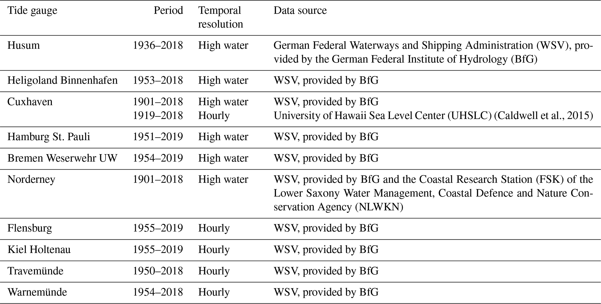
We used historic and real-time water level measurements from 10 tide gauges along the German North Sea and Baltic Sea coasts and their estuaries (Fig. 1) to set up the monitor. The data-processing workflow is illustrated in Fig. 2. The historic data were used to derive long-term statistics, while the real-time data were used to describe and measure the ongoing events. For the historic data, the available record length, temporal resolution, and source of the data vary (Table 1). Depending on that, we either used the twice-daily high water level or hourly data. When hourly data were available, information on the duration and intensity of extreme events could be derived. On the other hand, the maxima of extremes may be underestimated due to the sampling frequency. Only tide gauges with available records starting no later than the 1950s were selected.
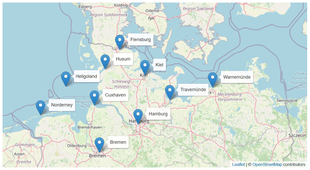
Figure 1Locations of the tide gauges used in the monitor. (Credit: Leaflet and maps © OpenStreetMap contributors. Distributed under a Creative Commons BY-SA License.)
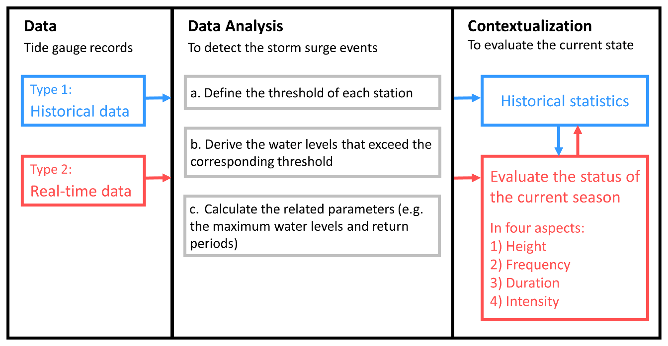
Table 1Summary of the tide gauge records used to calculate the long-term statistics.
Real-time data for all tide gauges are available every minute and are automatically fetched four times daily from PEGELONLINE (https://pegelonline.wsv.de, last access: 14 January 2022). They are subsequently resampled to either high water levels or hourly values depending on and matching the temporal resolution of available historical data at each tide gauge. All tide gauges measure relative to a land-based reference frame (relative sea level), and the data contain contributions from atmospheric and oceanic dynamics as well as from solid-Earth processes (Stammer et al., 2013). As it is relative sea level that is important for coastal management and protection (Rovere et al., 2016; Stammer et al., 2013), in our analyses the data are therefore intentionally not decomposed or detrended to retain contributions from sea level rise or subsidence.
2.3 Near-real-time data processing and information provision
To ensure near-real-time information provision, the monitor is automatically updated four times daily at 01:30, 07:30, 13:30, and 19:30 CET. When the water level within the last fetched period exceeds a gauge-specific threshold, a new storm surge event at this particular gauge is detected. Subsequently, new plots are automatically generated to provide the latest information and a near-real-time assessment of the event and its long-term and seasonal contextualization. While the availability of such an assessment represents the major purpose of the monitor, it has some limitations caused by potentially undetected errors in the real-time data. Since real-time data are normally raw data from measurements, it is possible and unavoidable that, for example, due to instrument failures during a storm no or only erroneous data are accessible, which could then affect the detection and classification of an extreme. Also, other technical problems can occur that lead to unusable values over extended periods. For example, the tide gauge at Norderney experienced a technical problem from May to September 2018. The measurements during that period were initially invalid with randomly high, low, or missing values, and a corresponding notification was posted on the PEGELONLINE website. To deal with such erroneous data in near real time, a quick quality control algorithm was implemented that marks and removes measurements whose absolute values of minute increments exceeded 0.3 m (spikes) or had values that were not within a reasonable range of 1–12 m. When updated quality-controlled data become available, new plots are produced, and figures and assessments may change compared to the initial near-real-time assessment.
2.4 Detection of storm surge events
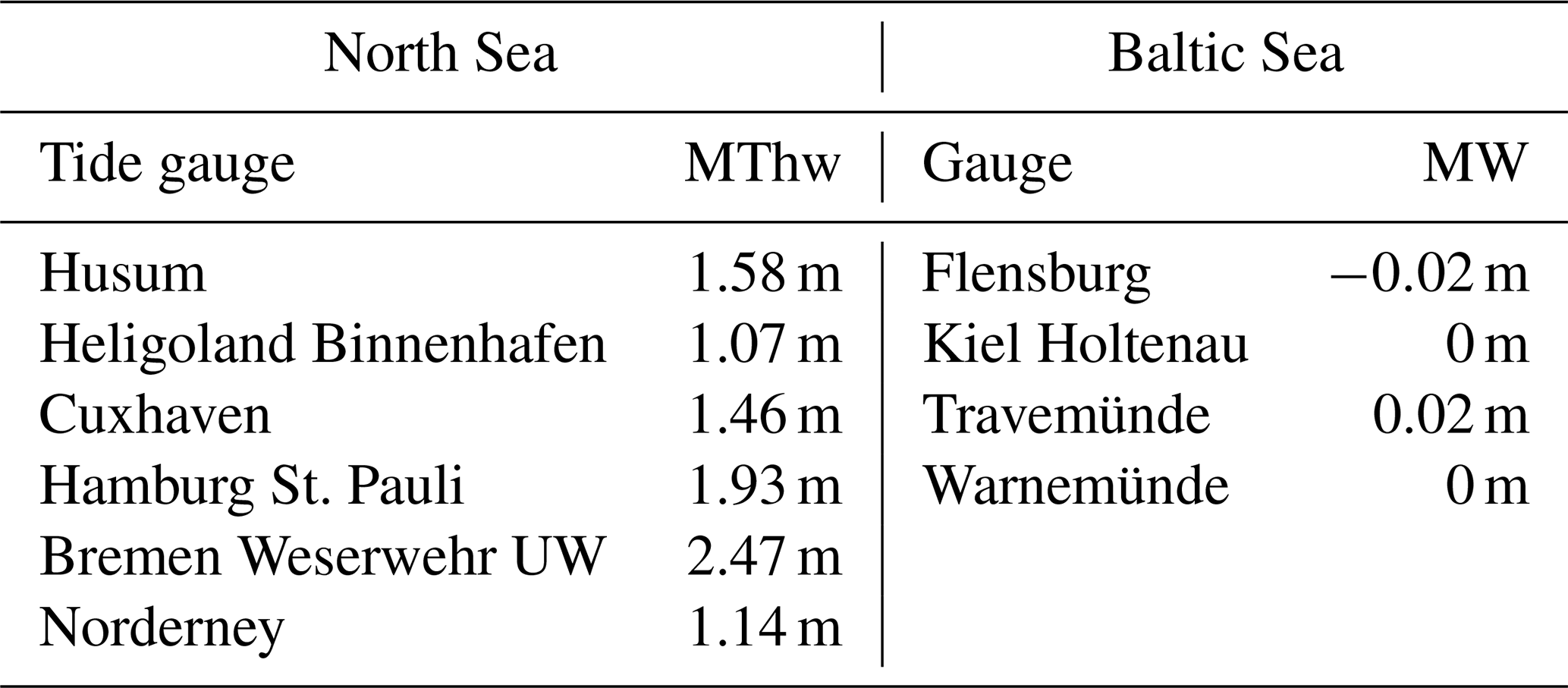
An important step in detecting and assessing storm surges is the definition of corresponding thresholds for the extremes. For the German North Sea and Baltic Sea coast, there are two different methods used in practice. The DIN 4049-3 standard defines a storm surge as an event in which regionally defined thresholds are exceeded. These thresholds are defined such that an event with a specific severity can be expected on average once for a given period, e.g., the once-in-20-years event (DIN 4049-3, 1994). For their forecasts and to issue public storm surge warnings, on the other hand, the German Federal Maritime and Hydrographic Agency (Bundesamt für Seeschifffahrt und Hydrographie, BSH) uses uniform exceedance thresholds for larger regions (Gönnert, 2003). While each method has advantages and disadvantages, the thresholds from the BSH were used in this study, as they are used in public warnings. Accordingly, for the German North Sea coast, a storm surge event is detected when the water level exceeds the local mean tidal high water level (MThw, Table 2) by at least 1.5 m. The event is subsequently further classified as a severe or very severe event when its maximum water level exceeds MThw by at least 2.5 or 3.5 m. Because of the different atmospheric and oceanographic conditions, storm surges at the German Baltic Sea coast are divided into four classes. Events in which the maximum water level exceeds the mean water level (MW) by 1.00 m are referred to as storm surge events. Events with water levels of 1.25–1.50 m above MW or 1.50–2.00 m above MW are referred to as medium or severe events. Cases in which the maximum water level is higher than 2.00 m above MW are referred to as very severe events. While for routine practices, mean tidal high water levels and mean water levels are regularly updated, we used fixed values calculated over the common reference period 1961–1990 (Table 2) so that events at all gauges can be compared, changes over a longer period can be monitored, and results are presented relative to a fixed reference. In the following, the period 1961–1990 is referred to as the reference period in the analyses.
Table 2Mean tidal high water levels (MThw) and mean water levels (MW) in meters relative to the German reference level NHN (Normalhöhennull) of the reference period 1961–1990 for the tide gauges along the North Sea and Baltic Sea coasts.
2.5 Definition of storm surge seasons
At the German North Sea and Baltic Sea coasts, storm surge activity is most pronounced in the winter season from October to March (Jensen and Müller-Navarra, 2008). In the monitor, the period from July to June of the following year was therefore used to define and characterize a storm surge season. Each storm surge season is denoted by the year in which the season ends. For instance, the period from July 2018 to June 2019 is referred to as season 2018/2019 and marked as 2019 in the plots. The course of a storm surge season and the monthly distributions are also derived and shown from July to June of the following year. When the ongoing season ends, new long-term statistics are automatically computed, in which the statistics of the concluded season will be included.
2.6 Main features presently implemented
The monitor was implemented for 10 tide gauges so far. Four of them are located at the German North Sea coast; two of them are in the Elbe and Weser estuaries; and four of them are along the German Baltic Sea coast (Fig. 1). For each tide gauge, a web page is generated providing figures, texts, and interpretations illustrating (a) the average conditions during the reference period and (b) their long-term trend. Recent storm surges are contextualized within the long-term development, and the ongoing storm surge season is compared to the reference period. Depending on the availability of historical data, different measures and statistics are available for each tide gauge. Information on storm surge height and frequency is presented for all gauges, while information on their duration and intensity is provided only for the gauges where historic hourly data exist (Cuxhaven, Flensburg, Kiel, Travemünde, and Warnemünde). To illustrate the main features of the monitor, the figures of the season 2019/2020 at the tide gauge Cuxhaven are discussed exemplarily.
2.6.1 Storm surge height
Information on two height indicators is provided, the development of the annual maximum water level over time and the return period of extremes (Fig. 3). Specifically, the maximum water level of the current season (red dot) is compared with the variations of the annual maxima of the previous seasons (black curve) (Fig. 3a). The plot allows for a quick visualization of the observed long-term changes and the extent to which the highest water level in the ongoing season is unusual. For an easy visualization, the current season is highlighted in all the annual plots by a vertical red-dotted line. The gray line provides an estimate of the linear trend with the gray-shaded area representing the 95 % confidence interval. The trend line is shown in solid when the estimated trend is significantly different from zero at the level of 95 % and dashed otherwise. The scale on the left axis is labeled as the water level relative to the German reference level (Normalhöhennull, NHN), while the right axis is labeled about the severity classification of storm surges (water level relative to MThw for the North Sea coast or relative to MW for the Baltic Sea coast).
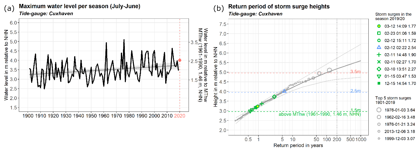
Figure 3(a) Maximum water level per storm surge season (past seasons – black; ongoing season – red) in meters (left ordinate: relative to NHN; right ordinate: relative to MThw of the reference period) and corresponding linear trend at Cuxhaven (gray line) together with the 95 % confidence interval (light-gray band). (b) Return periods of storm surge events at Cuxhaven from the past (gray symbols) and the ongoing season (colored symbols; green – minor; blue – severe; red – very severe events) together with the estimated distribution (dark-gray curve) and the corresponding 95 % confidence band (area between the light-gray curves) derived from past annual maxima. The events of the ongoing season and the top five severe historical events in the available period are listed on the right. Please note that the date formats in this figure are month-day and year-month-day.
The second plot provides estimates of the return periods of the storm surges that have occurred in the current ongoing season (Fig. 3b). Return periods are widely used to estimate the likelihood and severity of extreme events (e.g., Haigh et al., 2015; Wahl et al., 2017). To estimate the return period of storm surges, we fitted a generalized extreme value (GEV) distribution to the annual maximum values (Hennemuth et al., 2013). Here annual maxima refer to the block maxima within the historic storm surge seasons. The parameters of the distribution (location, scale, and shape) were derived by using the maximum-likelihood estimation (MLE).
Figure 3b displays the extreme value distribution (dark-gray curve) estimated from the historical data for Cuxhaven together with its 95 % confidence interval (two light-gray lines). This fit is subsequently used to evaluate the return period of the latest (ongoing) storm surges in near real time. When an event occurs, a colored symbol whose color denotes its severity (green – minor; blue – severe; red – very severe) is added. Additionally, an entry on the top of the list of current events is generated (right). In the example season (Fig. 3b), several smaller events with return periods of less than 5 years and a larger event with a return period between about 5–10 years can be identified. To further put the recent events into perspective, a list of the five severest historical events during the available period (seasons 1901–2019 here) is given below the list of events of the current season. These are represented by gray open circles with different sizes indicating their magnitudes.
2.6.2 Storm surge frequency
Similarly, two plots assessing the frequency of storm surges are generated (Fig. 4). To visualize the long-term development, variability, and change, the number of storm surges per season over time is shown together with its trend (Fig. 4a). Generally, in all plots, a trend that is/is not different from zero at the 95 % confidence level is shown by a solid/dashed line. The severity of the events is marked with different colors to illustrate the number of events in the different severity classes in each season. Again the current season is highlighted in red. While still ongoing, it can already and preliminarily be put into context with previous seasons, long-term variability, and change.
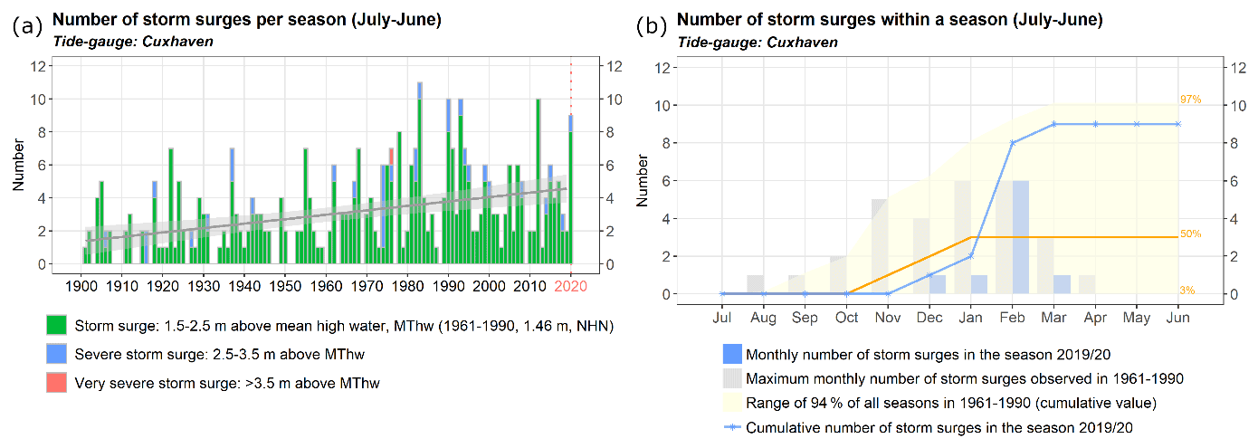
Figure 4(a) Number of storm surges per season (colored bars; green – minor; blue – severe; red – very severe) and the corresponding linear trend (gray line) together with the 95 % confidence band (gray shaded) at Cuxhaven. (b) Development of the ongoing storm surge season illustrated by the number of storm surges per month (blue) and their sum since the onset of the season (blue line) at Cuxhaven. For contextualization, also the historical monthly maximum number of events (gray bars) and the 50th percentile (orange curve) and the range between the 3rd and 97th percentiles (yellow-shaded area) from the cumulative number of events in the reference period 1961–1990 are shown.
The second plot (Fig. 4b) was designed to illustrate the course of the ongoing season. It can be used to assess, for example, if the onset of a storm surge season was very early or late, if there was an unusual number of events within a particular month, or if the whole season is unusually active or inactive compared to the average annual cycle. For this, the number of events in each month of the current season (blue bars) can be compared with the maximum number of events in the corresponding month over the reference period (1961–1990, gray bars). Further, the blue curve shows the cumulative number of events from the beginning of the current season until the day of the website visit. It can be compared to the reference given by the 50th percentile (orange curve) and the range between the 3rd and the 97th percentiles (yellow-shaded area) of the reference period. For example, when the blue curve remains below the orange one, this indicates that fewer events than usual were observed so far. If the blue curve is above the orange line but still within the yellow-shaded area, this suggests that the frequency of such a season is still within a normal range but already belongs to the more active ones. If the blue curve exceeds the yellow-shaded area, indications for an exceptionally active season do exist.
2.6.3 Storm surge duration and intensity
In addition to storm surge height and frequency, duration and intensity are widely used measures to describe the characteristics of storm surges (Cid et al., 2016; Zhang et al., 2000) that are also important from the perspective of coastal protection and risk management (e.g., Kodeih et al., 2019). Therefore, information on both measures was included in the monitor, although it can only be provided for those tide gauges where long-term hourly data were available. In the following analyses, duration denotes the number of hours for which the water level exceeds the given storm surge threshold, while intensity refers to the area between the water level measurements and the storm surge threshold and has units of meter × hour (m h). Regarding storm surge duration, the seasonal sum is a key indicator for coastal erosion. Regarding intensity, the maximum intensity of storm surges in a season is also critical for potential damages to coastal infrastructure.
In the monitor, the total duration and the maximum intensity of storm surges in each season are both shown within a long-term context (Fig. 5). In both cases, the current season is highlighted with an orange bar to be easily separable from the previous seasons (gray bars). Assessment of single events within a season can be derived from Fig. 5c and d, in which the events of the current seasons (red dots) are shown relative to the monthly distributions derived from historical data. The historical reference (blue) is illustrated in the form of a box plot bounded by the 3rd and 97th percentiles. The median is given by the solid horizontal blue line, and the historical maximum in each month is denoted by the blue dot. Assessment can be obtained from the relative positions of the red dots, which indicate whether an event lasted longer or was more intense in comparison to the monthly statistics of the reference period.
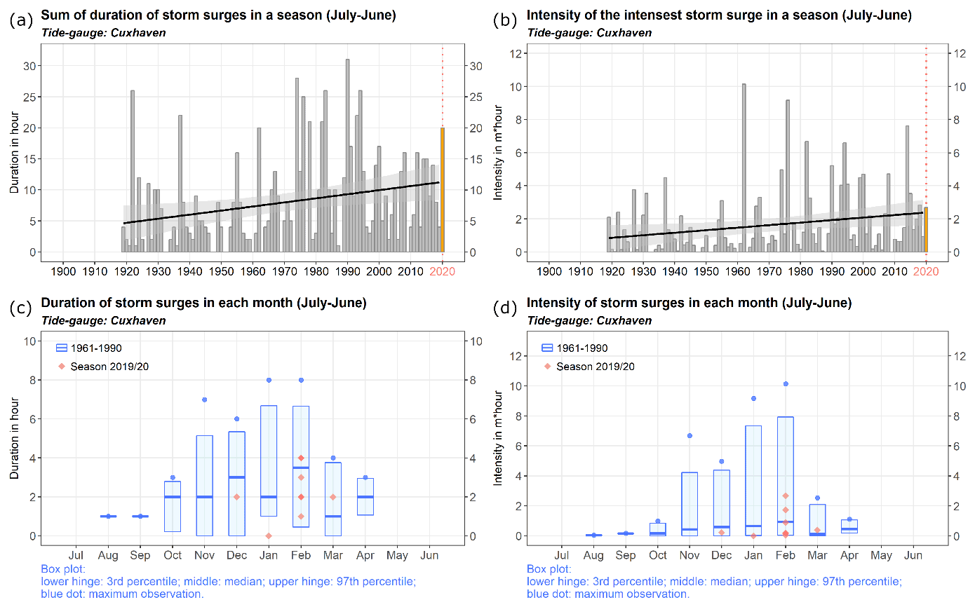
Figure 5(a, b) Total duration and maximum intensity of storm surges per season at Cuxhaven for past (gray bars) and the ongoing (orange bar) seasons together with the linear trend (black line) and the 95 % confidence interval. (c, d) Box plots for the monthly duration and intensity of storm surges in the reference period (blue box – 3rd to 97th percentile; blue line – median; blue point – maximum) together with the events of the ongoing season (orange).
In this section, the capabilities of the monitor in supporting assessments of long-term changes are briefly illustrated.
3.1 North Sea coast
3.1.1 Height
The annual maximum water level increased at all tide gauges over the available periods (e.g., Figs. 3a, 6). Except for Heligoland, the trends are significantly different from zero at the 95 % confidence level. The mean increase of the annual maximum water level since 1950 is about 20–40 cm at the coastal gauges and about 60–100 cm at the estuarine gauges Bremen and Hamburg. The reasons for the increases are still discussed in the literature but are likely to be the result of the interplay between several factors, such as mean sea level rise, variability in the wind climate, astronomical tide cycles, and the implementation of hydro-engineering measures with different contributions at the coast and in the estuaries (e.g., von Storch and Woth, 2008; von Storch et al., 2008; Hein et al., 2021; Jensen et al., 2021).
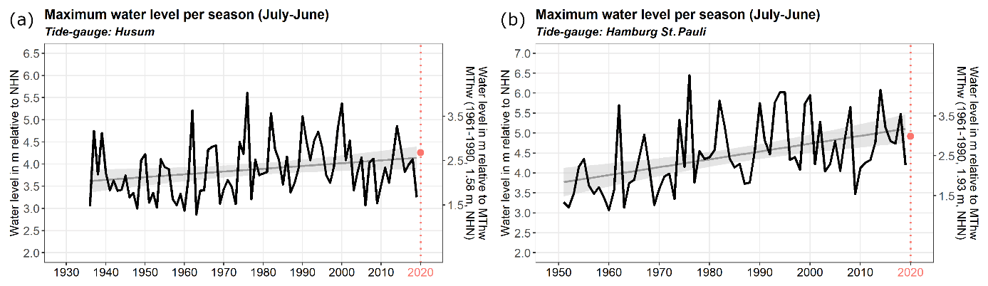
Although the trends are positive, the annual maximum water level strongly varies between seasons and from gauge to gauge. Among the gauges, either the storm surge of February 1962 (Heligoland, Bremen, and Norderney) or the storm surge of January 1976 (Husum, Cuxhaven, and Hamburg) is the highest since the beginning of data availability. Among the analyzed North Sea tide gauges, the highest water level since the 1950s occurred on 3 January 1976 at Hamburg St. Pauli with about 4.5 m above MThw. In the last decade, a storm surge in December 2013 represents the highest event. At some gauges (Cuxhaven, Hamburg, Bremen, and Norderney), it is among the five highest events over the available periods.
3.1.2 Frequency
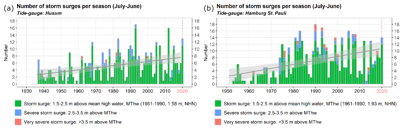
Annual storm surge frequency increased at all gauges (e.g., Figs. 4a, 7). Except for Heligoland, the trends are significantly different from zero at the 95 % confidence level. In the 1950s, about one to three storm surges usually occurred in a season. Over the past few decades, the annual number of storm surges has increased by about one at Heligoland and Norderney, and it has nearly doubled at Husum and Cuxhaven. At the estuarine gauges, storm surge frequency has increased even more strongly. On average, there are about 5 times as many storm surges per season nowadays as there were in the 1950s. In addition to the positive trends, the number of events also varies from season to season and from gauge to gauge. In general, there are fewer events at Heligoland, Cuxhaven, and Norderney, while events occur more frequently at Husum, Hamburg, and Bremen. This may be not only due to differences in the specific configuration of the coastline and bathymetry relative to the prevailing wind direction during storm surges that make a location more or less susceptible to storm surges (e.g., Gönnert, 2003) but also partly an effect of the common threshold used to detect surges in the monitor (see Sect. 2).
3.1.3 Duration and intensity
Due to the limited availability of high-temporal-resolution data, the statistics for storm surge duration and intensity can only be evaluated for Cuxhaven. As introduced in Sect. 2.6.3, the total duration of all events in a season and the intensity of the most intense event in a season are evaluated (Fig. 5a, b). For both measures, upward trends significantly different from zero could be inferred. Specifically, both measures have about doubled since the 1920s. The annual total duration increased from about 5 to 12 h, and the annual maximum intensity increased from about 1 m h to about 3 m h. This is likely caused by an increase in mean sea level that raised the baseline upon which wind-induced fluctuations act rather than a change in storm climate (e.g., Weisse et al., 2012; Weisse and Meinke, 2016). Averaged over the reference period, the mean values of the total duration and the maximum intensity were about 10 h and 2 m h, respectively.
3.2 Baltic Sea coast
3.2.1 Height
At the German Baltic Sea coast, the annual maximum water levels show strong variability over the available period. Linear trends within this period vary in their signs from gauge to gauge and because of the strong interannual variability; none of the trends is significantly different from zero at the 95 % confidence level (Fig. 8). This is consistent with the results based on annual data, which cover a longer period (e.g., Meinke, 1999). Although no significant changes in the extremes could be detected, the mean sea level has increased along the German Baltic Sea coast (e.g., Weisse and Meinke, 2016; Weisse et al., 2021) and is expected to rise further in the future (e.g., Grinsted, 2015; Hieronymus and Kalén, 2020). Therefore, it is likely that the annual maximum water levels may increase in the future as well. Thus, ongoing monitoring is important, although no significant trends in the annual maxima water level could be detected so far.
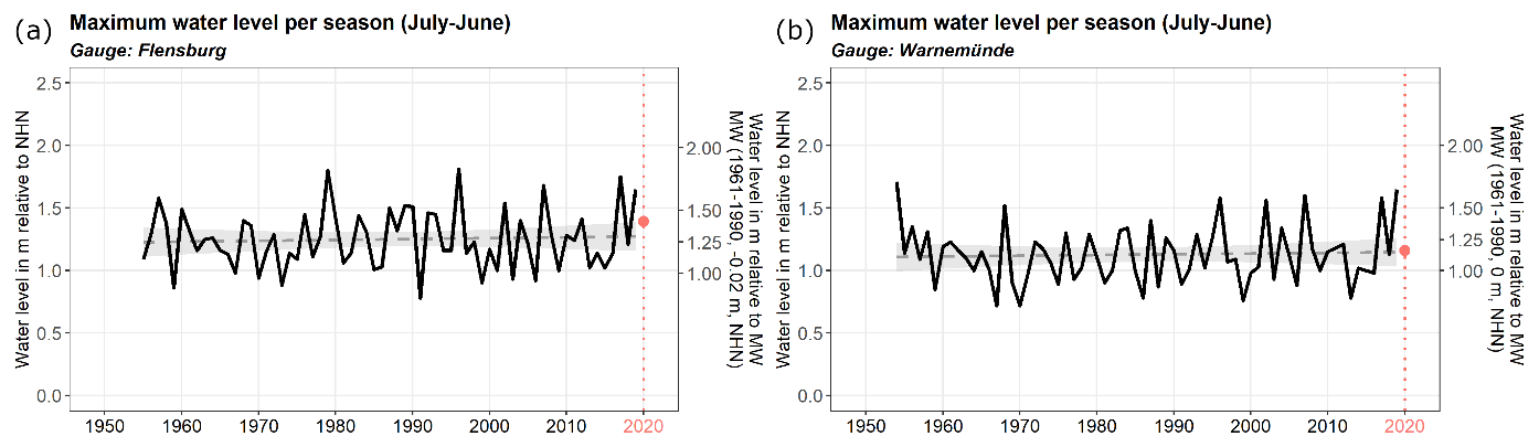
Over the past 7 decades, the annual maximum water level has varied between about 0.7 and 2.0 m above MW at the analyzed gauges. The average maximum water level is around 1.2 m above MW. The data in the monitor do not include the highest storm surge at the German Baltic Sea coast that occurred on 13 November 1872 (Jensen and Müller-Navarra, 2008; Rosenhagen and Bork, 2009; von Storch et al., 2015; Weisse and Meinke, 2016) and for which only limited reliable measurements are available. According to these, the maximum water level was about 3.3 m above MW (e.g., Jensen and Müller-Navarra, 2008) along the southwestern coast of the Baltic Sea. This is much higher than any extreme event that occurred later in this region. Since the 1950s, none of the water levels at the analyzed Baltic Sea gauges exceeded 2 m above MW (Fig. 8). However, this value was nearly hit in Travemünde on 4 January 1954 when the water level reached a value of 1.97 m above MW and in Kiel on 4 November 1995 when the water level reached a maximum of 1.96 m above MW (not shown).
3.2.2 Frequency
The storm surge frequency at the analyzed Baltic Sea gauges shows pronounced interannual and decadal variability. Over the available periods since the 1950s, the frequency has varied between zero and nine events. Except for Warnemünde, all gauges show a maximum of events observed in the season 1989/1990 (e.g., Flensburg, Fig. 9a). In Warnemünde the highest number of events in a season was five and was observed in 2001/2002 (Fig. 9b). Trends in storm surge frequency are not significant at all gauges (e.g., Fig. 9). As mean sea level increased over the period (e.g., Weisse et al., 2021), insignificant trends in the extremes may be due to the large interannual variability in the extremes that hamper detection in relatively short records. Overall, the storm climate over the area does not show significant trends (e.g., Weisse et al., 2021). This result is consistent with other studies analyzing different periods (e.g., 1883–1997 in Meinke, 1999, and 1948–2011 in Weidemann, 2014) and in which the effects of mean sea level rise have been excluded. Moreover, the wind climate over the Baltic Sea shows large interdecadal variability: for the last 6 decades, an increase in the number of days with westerly components has been detected during winter (Gräwe et al., 2019; Lehmann et al., 2011), while days with easterly winds have decreased (Gräwe et al., 2019). Since storm surges in the southwestern Baltic Sea are mainly connected with strong easterly winds, this variability in wind climate could further contribute to the insignificant trends in storm surge activity since 1950, against the background of rising mean sea level.

3.2.3 Duration and intensity
Information on duration and intensity can be derived at all selected Baltic Sea gauges, since hourly data are available. The total duration and the maximum intensity of storm surges per season show strong variabilities. Trends at all gauges vary around zero and are not statistically different from zero at the 95 % confidence level (Fig. 10). This is consistent with the findings from other studies that analyzed data from model hindcasts over different periods (e.g., Weidemann, 2014).
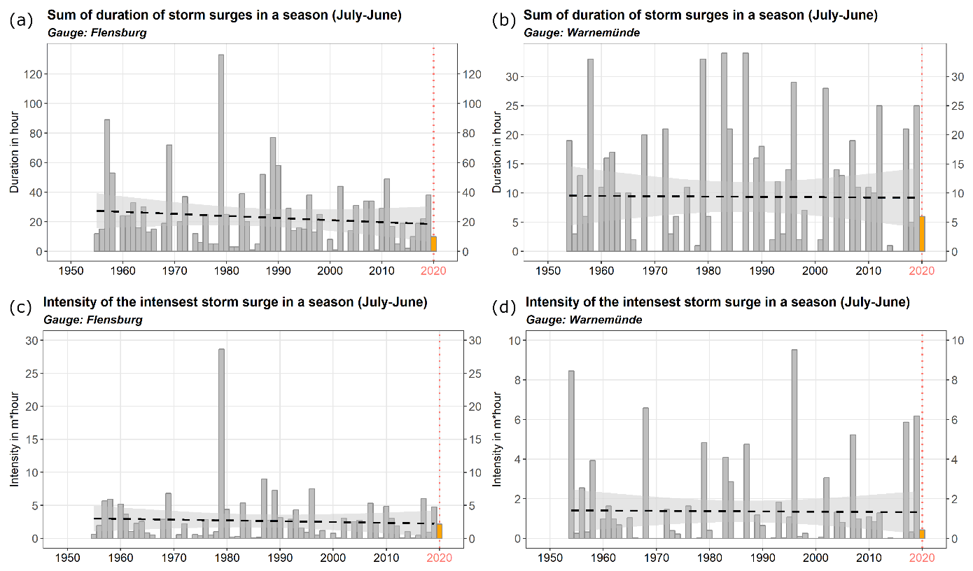
Figure 10(a, b) As Fig. 5a but for the gauges Flensburg (a) and Warnemünde (b). (c, d) As Fig. 5b but for the gauges Flensburg (c) and Warnemünde (d).
In this section, cases from two recent storm surge seasons (2018/2019 and 2019/2020) are exemplarily discussed to illustrate the capabilities of the monitor in aiding the identification of unusual events and/or seasons together with regional differences.
4.1 North Sea coast
4.1.1 Height
In the season 2018/2019, the annual maximum water levels at all gauges fell into the lowest category of severity (1.5–2.5 m above MThw) (e.g., Figs. 3a, 6). This immediately implies that all events observed in the season were minor (green marks in Fig. 11a, b). Except for Husum, the highest event in the season occurred on 8 January 2019, and its return period varies between about 1 and 3 years depending on the tide gauge. For Heligoland and Norderney, this was also the only event detected in this season using the thresholds defined in Sect. 2. It should be noted that the use of different thresholds (e.g., DIN 4049-3, 1994) can lead to different results. At other gauges, more events were registered, but they only slightly exceeded the lowest threshold (e.g., Husum and Hamburg in Fig. 11a, b). On average, such events may occur several times a year, and the season 2018/2019 was not unusual in terms of storm surge height.
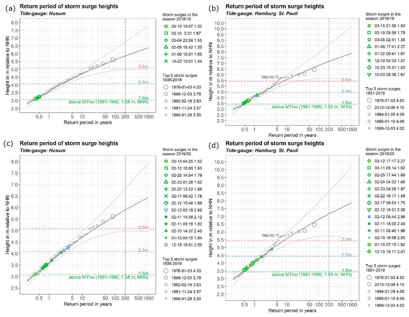
Figure 11As Fig. 3b but for the tide gauges Husum (a, c) and Hamburg St. Pauli (b, d): (a, b) season 2018/2019 and (c, d) season 2019/2020. Please note that the date formats in this figure are month-day and year-month-day.
Compared to the season 2018/2019, higher annual maximum water levels were observed in the following season, 2019/2020 (Figs. 3a, 6). During 10–12 February 2020, a storm named Sabine by the German Weather Service (Deutscher Wetterdienst) (Haeseler et al., 2020) and Ciara and Elsa by the UK Met Office and Norwegian Meteorological Institute, respectively, induced a series of consecutive storm surges. The highest water levels of the season were observed during these days. The estimated return period of the highest event varies from 3 to 8 years at different gauges (Fig. 11c, d). In addition to this series of events, more minor events were detected at Husum, Cuxhaven, Hamburg, and Bremen. They are categorized as minor events with estimated return periods shorter than 1 year, indicating that such minor events are common for these gauges. While somewhat more active than the previous season, again the season 2019/2020 was not unusual in terms of storm surge height.
4.1.2 Frequency
In terms of storm surge frequency, the two seasons 2018/2019 and 2019/2020 differ significantly. In the season 2018/2019, storm surge frequency is around the average frequency of the reference period. A total of one or two events was observed at Cuxhaven (Fig. 4a), Heligoland, and Norderney (not shown), whereas six events were observed at Husum (Fig. 12a), and eight events were observed at Hamburg (Fig. 12b) and Bremen (not shown).
In the season 2019/2020, the number of events was at least twice as high at five of the six tide gauges. Especially, the number of 13 events at Husum is remarkable and exceeds the 3rd–97th percentile of the reference period (Fig. 12c). The season ranks among the top three in terms of storm surge frequencies at this gauge (Fig. 7a).
A look at the course of the season and the long-term average reveal that the first storm surges usually occur in November or December and that the majority occur between November and February (Fig. 12). The course of the season 2018/2019 broadly followed this development along the long-term median (Fig. 12a, b). For some gauges, frequencies eventually exceeded the long-term median, but the values remained well below the 97th percentiles. Moreover, the numbers of events in the individual months were exceptional nowhere.

Figure 12As Fig. 4b but for the tide gauges Husum (a, c) and Hamburg St. Pauli (b, d): (a, b) season 2018/2019 and (c, d) season 2019/2020.
In contrast, the season 2019/2020 was substantially different. The season initially started late, and the storm surge frequencies were moderate and mostly below the long-term median. This character substantially changed in February when the storm Sabine caused a large number of events within a relatively short period (Fig. 12c, d). For example at Husum, nine events (five of which were caused within only about 2 d) were registered in February 2020, which exceeds the maximum of seven events detected so far in February (Fig. 9c). Consequently, the cumulated number of events in the season exceeds the 3rd–97th percentile range, and the season eventually represented a rather unusual season in terms of storm surge frequency, although their height was mostly moderate.
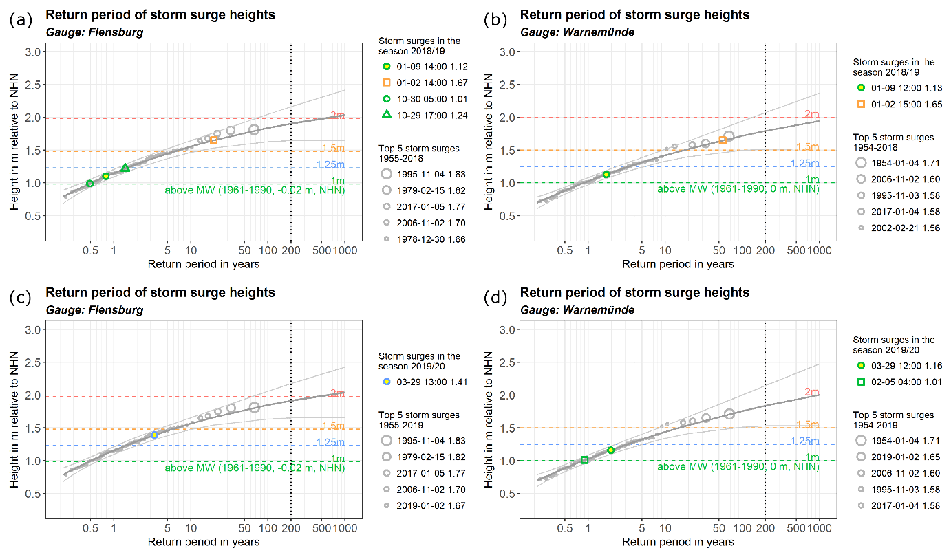
Figure 13As Fig. 3b but for the gauges Flensburg (a, c) and Warnemünde (b, d): (a, b) season 2018/2019 and (c, d) season 2019/2020. Please note that the date formats in this figure are month-day and year-month-day.
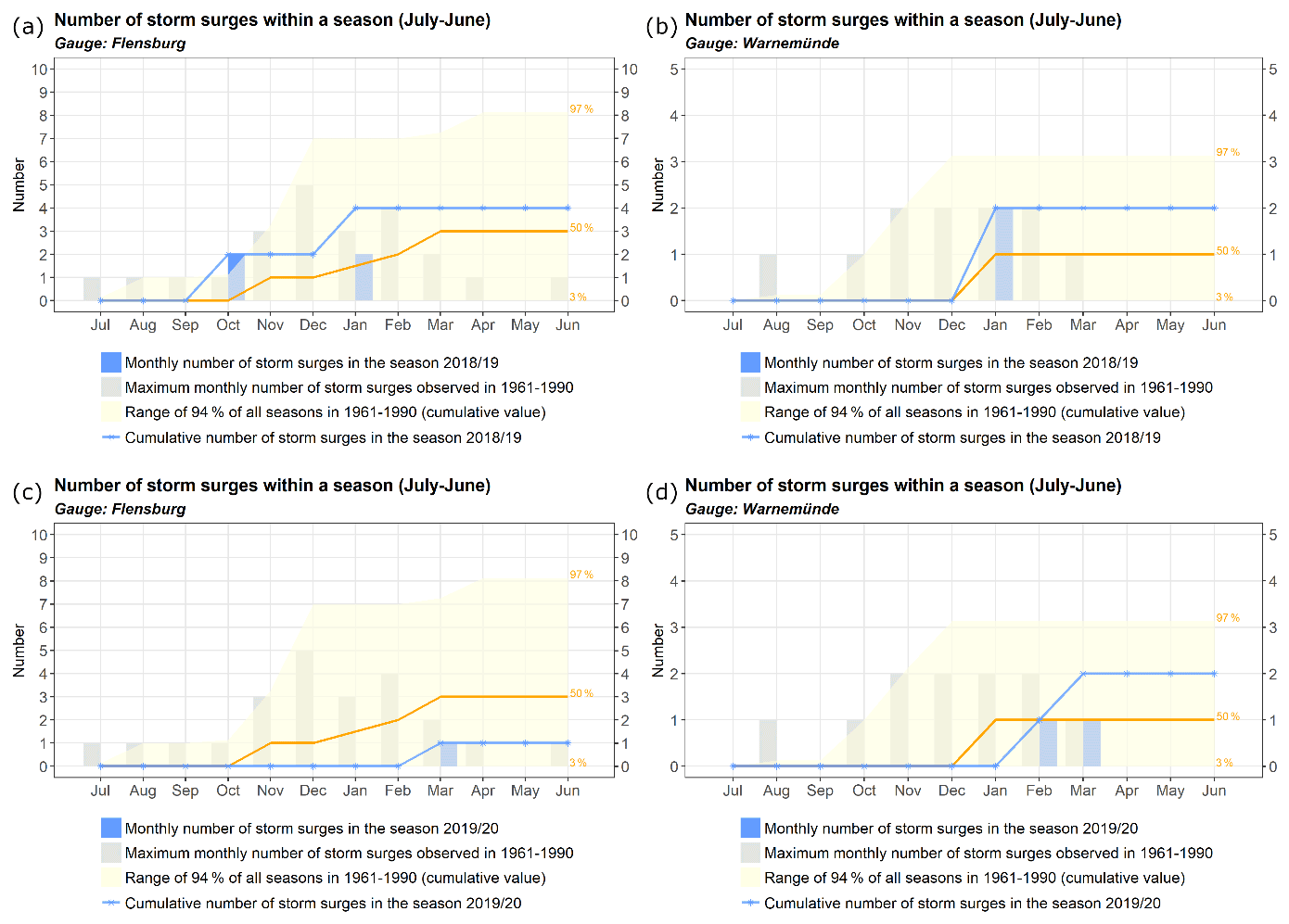
Figure 14As Fig. 4b but for the gauges Flensburg (a, c) and Warnemünde (b, d): (a, b) season 2018/2019 and (c, d) season 2019/2020.
4.1.3 Duration and intensity
The two storm surge seasons also differ in terms of their total duration and their maximum intensity. This is demonstrated exemplarily for Cuxhaven (Fig. 5). Here, both measures were significantly higher in the season 2019/2020, especially the total duration. In this case, this can be attributed to the unusually large number of shorter events in this season (see discussion above), while the individual events were neither exceptionally intense nor long-lasting (Fig. 5c, d).
In summary, for the German North Sea coast, the storm season 2018/2019 represents a rather typical storm surge season in all aspects. All detected events were relatively low, and their return periods were mostly shorter than 1 year. Although the number of events at some gauges was slightly above the average level, it is still far from the upper bound defined by the long-term 97th percentile. In contrast, the season 2019/2020 was more active and unusual in some aspects. It was characterized by a slow onset, which was more than compensated by an unusual series of events in February. In consequence, the total number of events at the end of the season was only slightly below or even above the upper bound of the long-term distribution. While the surges were mostly moderate in height, the total duration of the storm surges was also doubled compared to the reference period.
4.2 Baltic Sea coast
4.2.1 Height
Contrary to the North Sea where the two storm surge seasons 2018/2019 and 2019/2020 were rather similar in height but differed in frequencies, both seasons differed in height in the Baltic Sea with the first season being the stronger one. This illustrates that in both areas different meteorological conditions are required to generate storm surges. The differences between both seasons are shown exemplarily for Flensburg and Warnemünde (Fig. 13). At both gauges, the highest storm surge in the season 2018/2019 occurred on 2 January 2019 and was caused by the storm Zeetje (Perlet, 2019). The maximum water levels reached 1.67 and 1.65 m, respectively, at Flensburg and Warnemünde. In both cases, the event represented severe storm surges. In Warnemünde its height was very close to the highest value of 1.71 m in the record, and the estimated return period of the event in January 2019 was between about 50–60 years. At the other gauges, the frequency of such events is somewhat larger, and the return periods of the January 2019 event vary between about 10–20 years. Regarding height, the season 2019/2020 was less active with events having return periods well below 5 years (Fig. 13).
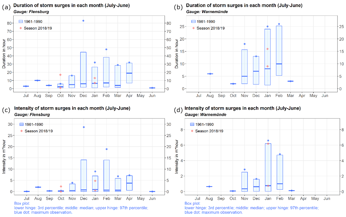
Figure 15(a, b) As Fig. 5c but for the gauges Flensburg (a) and Warnemünde (b). (c, d) As Fig. 5d but for the gauges Flensburg (c) and Warnemünde (d).
4.2.2 Frequency
In contrast to the North Sea, both seasons in the Baltic Sea were relatively typical in terms of storm surge frequency. This is again shown exemplarily for Travemünde and Warnemünde (Fig. 14). While in 2018/2019 the storm surge frequency at both gauges was slightly above the average of the reference period, in 2019/2020 it was below average in Flensburg and above average in Warnemünde. In all cases, values fell within usual ranges, except for the maximum number of surges observed in October 2018 in Flensburg. Note, however, that total numbers are small, which makes comparisons less robust.
4.2.3 Duration and intensity
Contrary to the North Sea, the season 2018/2019 was more active than 2019/2020 in terms of total duration and intensity (Fig. 10). While for the North Sea, the season 2019/2020 was outstanding in terms of duration due to a series of moderate events, for the Baltic Sea the season 2018/2019 stands out in terms of intensity caused by a major event in January 2019 (Fig. 15). In Flensburg also the duration and intensity of the event on 29 October 2018 were exceptionally high (Fig. 15a, c). Again this illustrates that different atmospheric conditions are required to trigger storm surges along the German North Sea and Baltic Sea coasts.
A new tool and approach for monitoring the storm surge hazard in the context of long-term variability and climate change were proposed. They aim at providing near-real-time information for the evaluation and contextualization of ongoing extremes and at bridging the gap between the availability of real-time data and the considerable time delay before assessments are published. The approach was implemented into a prototype web tool (the storm surge monitor) and implemented exemplarily for the German North Sea and Baltic Sea coasts. With the help of the monitor, storm surges are detected in real time and are set into a climatological context in near real time. This way, not only an assessment of the current storm surge season or ongoing events is achieved, but also the development over the past seasons is documented. The tool aims at providing easily accessible information to the public, scientists, and stakeholders that aid in the evaluation of extremes, for example, to assess in near real time if and to what extent an event or a season is unusual compared to the statistics of the extreme events in the past decades. Measures to assess long-term changes can also be inferred from the monitor. Because of the existing risk and the expected future developments, such information can be highly relevant for decision making (e.g., Kodeih, 2018; Kodeih et al., 2019; Weisse et al., 2015) or within public debate.
The monitor also documents long-term changes in storm surge climate. Such changes can in principle originate from various factors, such as changes in storm activity, astronomical tide cycles, or sea level rise. Locally, waterworks may also play a role. To date, there is no clear evidence suggesting a significant long-term change of storm activity in the German coastal regions (Feser et al., 2015; Krieger et al., 2020; Krueger et al., 2019; Stendel et al., 2016; Weisse et al., 2012). For the North Sea gauges, likely, the observed changes in storm surge climate are largely related to the local mean sea level rise (e.g., Weisse et al., 2012; Woodworth et al., 2011). Rising relative sea levels in the area, for the most part, not only are related to global mean sea level rise and climate change but also contain contributions from non-climatic factors such as land subsidence. The latter may result from natural phenomena (e.g., GIA) or local anthropogenic activities (e.g., groundwater extraction, dredging, or waterworks) (e.g., Rovere et al., 2016; Stammer et al., 2013; Tamisiea and Mitrovica, 2011).
At the analyzed gauges at the German Baltic Sea coast, no significant long-term change in storm surge activity has been detected so far. For the annual maximum water levels, this is in agreement with, e.g., the results of Meinke (1999) and the review in Weisse et al. (2021). Similarly, non-significant trends have been found for storm surge frequency, also in agreement with previous studies (e.g., Weidemann, 2014).
It is plausible that storm surge height, frequency, duration, and intensity may change in the future, as sea level continues to rise along the German North Sea and Baltic Sea coasts (e.g., Grinsted, 2015; Weisse and Meinke, 2016; Hieronymus and Kalén, 2020; Weisse et al., 2021). Thus, continuous monitoring of the storm surge climate in a climatological context may foster early detection and attribution and support adaptation and public debate.
Nowadays, web-based applications are frequently used tools to develop links between the results of scientific research and public demands. For sea level extremes, various such efforts do exist. These tools provide online access to the statistics of extreme water levels or document the severity and consequences of historical flooding. Examples are the Extreme Water Levels site from NOAA (https://tidesandcurrents.noaa.gov/est/, last access: 14 January 2022) or the SurgeWatch site for the UK coast (https://www.surgewatch.org/, last access: 14 January 2022, Haigh et al., 2015). We built upon experiences from developing such tools, but contrary to existing ones our storm surge monitor focuses on the near-real-time evaluation and contextualization of extremes against the background of long-term variability and change to provide an up-to-date and continuously available piece for coastal climate services. Both the monitor and the statistics are freely available online. They are expected to be useful and meaningful to the public. In particular, the monitor was found to be useful to the media, since it fits their needs to focus on actual threats and to contextualize them within a scientific frame. After the implementation of the monitor, numerous interview requests were served and background information was provided based on the monitor.
The monitor is further relevant to multi-sector coastal stakeholders who demand such information for coastal flood risk management and planning. For example, presently a discussion is ongoing with users asking for an extension including also thresholds following the definitions given in the DIN 4049-3 standard (DIN4049-3, 1994). Further and interestingly, the series of storm surges that made the season 2019/2020 outstanding along the North Sea coast occurred shortly after the conclusion of the transdisciplinary project EXTREMENESS (Weisse et al., 2019) in which physically plausible but yet unobserved extremes and their potential impacts were discussed and modeled. One type of such potentially high-impact events identified by stakeholders was a series of storm surges that, even when only of moderate heights, may provide challenges for coastal protection (Schaper et al., 2019; Weisse et al., 2019).
The monitor can further serve for educational purposes, for example, illustrating changing storm surge activity at German coasts. Finally, it can also be useful to researchers as auxiliary information supporting their research. We argue that the tool has the potential to be developed into a larger suite of tools including, for example, other regions or other coastal hazards such as sea level rise or storm activity.
The code used for data pre- and post-processing is available on request from the authors.
The data used in this paper are available from the third party sources listed in Table 1. Real-time data are available from https://www.pegelonline.wsv.de/ (PEGELONLINE, 2022) as described in the text. Near-real-time analyzes are available from the monitor websites in German (https://sturmflut-monitor.de, STURMFLUT-MONITOR, 2022) and in English (https://stormsurge-monitor.eu, STORMSURGE-MONITOR, 2022).
RW and IM initiated the idea of the storm monitor and designed it. XL processed the data, performed the analyses, and programmed the web tool. All authors equally contributed to the preparation of the manuscript. The revised version including the suggestions from the reviewers was prepared by RW and IM.
The contact author has declared that neither they nor their co-authors have any competing interests.
Publisher’s note: Copernicus Publications remains neutral with regard to jurisdictional claims in published maps and institutional affiliations.
The map in Fig. 1 is generated by Leaflet and © OpenStreetMap contributors.
This work was financially supported by the European Union through the project “European advances on CLImate Services
for Coasts and SEAs” (ECLISEA) under the ERA4CS (European Research Area for Climate Services) framework (EU grant agreement no. 690462).
The article processing charges for this open-access publication were covered by the Helmholtz-Zentrum Hereon.
This paper was edited by Paolo Tarolli and reviewed by Klaus Grosfeld and Andreas Sterl.
Arns, A., Dangendorf, S., Jensen, J., Talke, S., Bender, J., and Pattiaratchi, C.: Sea-level rise induced amplification of coastal protection design heights, Sci Rep., 7, 40171, https://doi.org/10.1038/srep40171, 2017.
Barbosa, S. M.: Quantile trends in Baltic sea level, Geophys. Res. Lett., 35, L22704, https://doi.org/10.1029/2008gl035182, 2008.
Butler, A., Heffernan, J. E., Tawn, J. A., and Flather, R. A.: Trend estimation in extremes of synthetic North Sea surges, J. Roy. Stat. Soc. C.-App., 56, 395–414, https://doi.org/10.1111/j.1467-9876.2007.00583.x, 2007.
Caldwell, P. C., Merrifield, M. A., and Thompson, P. R.: Sea level measured by tide gauges from global oceans – the Joint Archive for Sea Level holdings (NCEI Accession 0019568), Version 5.5, NOAA National Centers for Environmental Information [data set], https://doi.org/10.7289/V5V40S7W, 2015.
Cid, A., Menendez, M., Castanedo, S., Abascal, A. J., Mendez, F. J., and Medina, R.: Long-term changes in the frequency, intensity and duration of extreme storm surge events in southern Europe, Clim. Dynam., 46, 1503–1516, https://doi.org/10.1007/s00382-015-2659-1, 2016.
Dangendorf, S., Müller-Navarra, S., Jensen, J., Schenk, F., Wahl, T., and Weisse, R.: North Sea storminess from a novel storm surge record since AD 1843, J. Climate, 27, 3582–3595, https://doi.org/10.1175/jcli-d-13-00427.1, 2014.
Deutschländer, T., Friedrich, K., Haeseler, S., and Lefebvre, C.: Severe storm XAVER across northern Europe from 5 to 7 December 2013, Deutscher Wetterdienst, available at: https://www.dwd.de/EN/ourservices/specialevents/storms/20131230_XAVER_europe_en.pdf?__blob=publicationFile&v=20131234 (last access: 14 January 2022), 2013.
DIN 4049-3: Hydrologie. Teil 3: Begriffe zur quantitativen Hydrologie 135DVWK (Deutscher Verband für Wasserwirtschaft und Kulturbau) (1999): Statistische Analyse von Hochwasserabflüssen, DVWK 215/1999, Verlag Paul Parey, Hamburg, https://doi.org/10.31030/2644617, 1994.
Feser, F., Barcikowska, M., Krueger, O., Schenk, F., Weisse, R., and Xia, L.: Storminess over the North Atlantic and northwestern Europe – A review, Q. J. Roy. Meteor. Soc., 141, 350–382, https://doi.org/10.1002/qj.2364, 2015.
Feuchter, D., Jörg, C., Rosenhagen, G., Auchmann, R., Martius, O., and Brönnimann, S.: The 1872 Baltic Sea storm surge, in: Weather extremes during the past 140 years, edited by: Brönnimann, S. and Martius, O., Geographica Bernensia G89, https://doi.org/10.4480/GB2013.G89.10, 2013.
Gaslikova, L., Grabemann, I., and Groll, N.: Changes in North Sea storm surge conditions for four transient future climate realizations, Nat. Hazards, 66, 1501–1518, https://doi.org/10.1007/s11069-012-0279-1, 2013.
Gönnert, G.: Sturmfluten und Windstau in der Deutschen Bucht. Charakter, Veränderungen und Maximalwerte im 20. Jahrhundert, Die Küste, 67, 185–365, 2003.
Gönnert, G. and Buß, T.: Sturmfluten zur Bemessung von Hochwasserschutzanlagen, Landesbetrieb Straßen, Brücken und Gewässer 2/2009, ISSN 1867–7959, 2009.
Gräwe, U., Klingbeil, K., Kelln, J., and Dangendorf, S.: Decomposing Mean Sea Level Rise in a Semi-Enclosed Basin, the Baltic Sea, J. Climate, 32, 3089–3108, https://doi.org/10.1175/JCLI-D-18-0174.1, 2019.
Grinsted, A.: Projected Change – Sea Level, in: Second Assessment of Climate Change for the Baltic Sea Basin, edited by: The BACC II Author Team, Springer, Cham, https://doi.org/10.1007/978-3-319-16006-1_14, 2015.
Haeseler, S., Bissolli, P., Dassler, J., Zins, V., and Kreis, A.: Orkantief Sabine löst am 09./10. Februar 2020 eine schwere Sturmlage über Europa aus, DWD, available at: https://www.dwd.de/DE/leistungen/besondereereignisse/stuerme/20200213_orkantief_sabine_europa.pdf (last access: 14 January 2022), 2020
Haigh, I. D., Wadey, M. P., Gallop, S. L., Loehr, H., Nicholls, R. J., Horsburgh, K., Brown, J. M., and Bradshaw, E.: A user-friendly database of coastal flooding in the United Kingdom from 1915–2014, Sci. Data, 2, 150021 (2015), https://doi.org/10.1038/sdata.2015.21, 2015.
Hall, A.: The North Sea Flood of 1953, Environment & Society Portal, Arcadia, no. 5, Rachel Carson Center for Environment and Society, https://doi.org/10.5282/rcc/5181, 2013.
Hegerl, G. C., Hoegh-Guldberg, O., Casassa, G., Hoerling, M. P., Kovats, R. S., Parmesan, C., Pierce, D. W., and Stott, P. A.: Good Practice Guidance Paper on Detection and Attribution Related to Anthropogenic Climate Change, in: Meeting Report of the Intergovernmental Panel on Climate Change Expert Meeting on Detection and Attribution of Anthropogenic Climate Change, edited by: Stocker, T. F., Field, C. B., Qin, D., Barros, V., Plattner, G.-K., Tignor, M., Midgley, P. M., and Ebi, K. L., IPCC Working Group I Technical Support Unit, University of Bern, Bern, Switzerland, available at: https://archive.ipcc.ch/pdf/supporting-material/ipcc_good_practice_guidance_paper_anthropogenic.pdf (last access: 19 January 2022), 2010.
Hein, S. S. V., Sohrt, V., Nehlsen, E., Strotmann, T., and Fröhle, P.: Tidal Oscillation and Resonance in Semi-Closed Estuaries – Empirical Analyses from the Elbe Estuary, North Sea, Water, 2021, 848, https://doi.org/10.3390/w13060848, 2021
Hennemuth, B., Bender, S., Bülow, K., Dreier, N., Keup-Thiel, E., Krüger, O., Mudersbach, C., Radermacher, C., and Schoetter, R.: Statistical methods for the analysis of simulated and observed climate data, applied in projects and institutions dealing with climate change impact and adaptation, CSC Rep. 13, Climate Service Center, Germany, available at: https://www.climate-service-center.de/imperia/md/content/csc/projekte/csc-report13_englisch_final-mit_umschlag.pdf (last access: 14 January 2022), 2013.
Hieronymus, M. and Kalén, O.: Sea-level rise projections for Sweden based on the new IPCC special report: The ocean and cryosphere in a changing climate, Ambio, 49, 1587–1600, https://doi.org/10.1007/s13280-019-01313-8, 2020.
Hollebrandse, F. A. P.: Temporal development of the tidal range in the southern North Sea, master, MS thesis, Delft Univ. of Technol., Delft, The Netherlands, available at: http://resolver.tudelft.nl/uuid:d0e5cb29-1c09-4de3-a1e6-0b17a9cb43ec (last access: 14 January 2022), 2005.
Horsburgh, K. J. and Wilson, C.: Tide-surge interaction and its role in the distribution of surge residuals in the North Sea, J. Geophys. Res.-Oceans, 112, C08003, https://doi.org/10.1029/2006jc004033, 2007.
Hünicke, B. and Zorita, E.: Influence of temperature and precipitation on decadal Baltic Sea level variations in the 20th century, Tellus A, 58, 141–153, https://doi.org/10.1111/j.1600-0870.2006.00157.x, 2006.
Jensen, J. and Müller-Navarra, S. H.: Storm surges on the German coast, Die Küste, 74, 92–124, 2008.
Jensen, J., Ebener, A., Jänicke, L., Arns, A., Hubert, K., Wurpts, A., Berkenbrink, C., Weisse, R., Yi, X., and Meyer, E.: Untersuchungen zur Entwicklung der Tidedynamik an der deutschen Nordseeküste (ALADYN), Die Küste, 89, https://doi.org/10.18171/1.089105, 2021.
Karabil, S.: Influence of Atmospheric Circulation on the Baltic Sea Level Rise under the RCP8.5 Scenario over the 21st Century, Climate, 5, 71, https://doi.org/10.3390/cli5030071, 2017.
Karabil, S., Zorita, E., and Hünicke, B.: Mechanisms of variability in decadal sea-level trends in the Baltic Sea over the 20th century, Earth Syst. Dynam., 8, 1031–1046, https://doi.org/10.5194/esd-8-1031-2017, 2017.
Kodeih, S.: Catalogue of potential coastal climate indicators for a pan-European coastal climate service web tool, Deliverable 1.D, Work Package 1, Project ECLISEA, available at: https://www.ecliseaproject.eu/wp-content/uploads/2019/08/d1d_report_final.pdf (last access: 13 December 2021), 2018.
Kodeih, S., Cozannet, G. L., Maspataud, A., Meyssignac, B., Maisongrande, P., Ayerbe, I. A., Emmanouil, G., and Vlachogianni, M.: Climate information needs from multi-sector stakeholders, Deliverable 1.B, Work Package 1, Project ECLISEA, available at: https://www.ecliseaproject.eu/wp-content/uploads/2019/08/d1.b_report_stakeholder-needs_final_20180629.pdf (last access: 13 December 2021), 2019.
Krieger, D., Krueger, O., Feser, F., Weisse, R., Tinz, B., and von Storch, H.: German Bight storm activity, 1897–2018, Int. J. Climatol., 41, E2159–E2177, https://doi.org/10.1002/joc.6837, 2020.
Krueger, O., Feser, F., and Weisse, R.: Northeast Atlantic storm activity and its uncertainty from the late nineteenth to the twenty-first century, J. Climate, 32, 1919–1931, https://doi.org/10.1175/jcli-d-18-0505.1, 2019.
Lehmann, A., Getzlaff, K., and Harlaß, J.: Detailed assessment of climate variability in the Baltic Sea area for the period 1958 to 2009, Clim. Res., 46, 185–196, https://doi.org/10.3354/cr00876, 2011.
Meinke, I.: Sturmfluten in der südwestlichen Ostsee – dargestellt am Beispiel des Pegels Warnemünde, Marburger Geographische Schriften, 134, 1–23, 1999.
Meinke, I.: Stakeholder-based evaluation categories for regional climate services – a case study at the German Baltic Sea coast, Adv. Sci. Res., 14, 279–291, https://doi.org/10.5194/asr-14-279-2017, 2017.
Mudersbach, C. and Jensen J.: Statistische Extremwertanalyse von Wasserständen an der Deutschen Ostseeküste, in: Abschlussbericht 1.4 KFKI-VERBUNDPROJEKT Modellgestützte Untersuchungen zu extremen Sturmflutereignissen an der Deutschen Ostseeküste (MUSTOK), Universität Siegen, https://doi.org/10.2314/GBV:609714708, 2008.
Needham, H. F., Keim, B. D., and Sathiaraj, D.: A review of tropical cyclone-generated storm surges: Global data sources, observations, and impacts, Rev. Geophys., 53, 545–591, https://doi.org/10.1002/2014rg000477, 2015.
PEGELONLINE: Real-time data, available at: https://www.pegelonline.wsv.de/, last access: 14 January 2022.
Perlet, I.: Ostsee-Sturmflut am 02.01.2019, Berichte zu Ostsee-Sturmfluten und -Hochwassern, BSH, available at: https://www.bsh.de/DE/THEMEN/Wasserstand_und_Gezeiten/Sturmfluten/_Anlagen/Downloads/Ostsee_Sturmflut_20190102.pdf?__blob=publicationFile&v=20190105 (last access: 14 January 2022), 2019.
Ratter, B. M. W. and Kruse, N.: Klimawandel und Wahrnehmung – Risiko und Risikobewusstsein in Hamburg, in: Klimawandel und Klimawirkung, edited by: Böhner, J. and Ratter, B. M. W., Hamburg 2010, Hamburger Symposium Geographie, Band 2, Institut für Geographie der Universität Hamburg, ISBN 9783980686594, 2010.
Ribeiro, A., Barbosa, S. M., Scotto, M. G., and Donner, R. V.: Changes in extreme sea-levels in the Baltic Sea, Tellus A, 66, 20921, https://doi.org/10.3402/tellusa.v66.20921, 2014.
Richter, A., Groh, A., and Dietrich, R.: Geodetic observation of sea-level change and crustal deformation in the Baltic Sea region, Phys. Chem. Earth, 53–54, 43–53, https://doi.org/10.1016/j.pce.2011.04.011, 2012.
Rosenhagen, G. and Bork, I.: Rekonstruktion der Sturmwetterlage vom 13. November 1872, Die Küste, 75, 51–70, 2009.
Rovere, A., Stocchi, P., and Vacchi, M.: Eustatic and relative sea level changes, Current Climate Change Reports, 2, 221–231, https://doi.org/10.1007/s40641-016-0045-7, 2016.
Rucińska, D.: Describing Storm Xaver in disaster terms, Int. J. Disast. Risk. Re., 34, 147–153, https://doi.org/10.1016/j.ijdrr.2018.11.012, 2019.
Schaper, J., Ulm, M., Arns, A., Jensen, J., Ratter, B., and Weisse, R.: Transdisziplinäres Risikomanagement im Umgang mit extremen Nordsee-Sturmfluten – Vom Modell zur Wissenschafts-Praxis-Kooperation, Die Küste, 87, 75–114, https://doi.org/10.18171/1.087112, 2019.
Stammer, D., Cazenave, A., Ponte, R. M., and Tamisiea, M. E.: Causes for contemporary regional sea level changes, Annu. Rev. Mar. Sci., 5, 21–46, https://doi.org/10.1146/annurev-marine-121211-172406, 2013.
Stendel, M., van den Besselaar, E., Hannachi, A., Kent, E. C., Lefebvre, C., Schenk, F., van der Schrier, G., and Woollings, T.: Recent change – Atmosphere, in: North Sea region climate change assessment, edited by: Quante, M. and Colijn, F., 55–84, https://doi.org/10.1007/978-3-319-39745-0_2, 2016.
STORMSURGE-MONITOR: Near-real-time analyzes, available at: https://stormsurge-monitor.eu, last access: 19 January 2022.
STURMFLUT-MONITOR: Near-real-time analyzes, available at: https://sturmflut-monitor.de, last access: 19 January 2022.
Tamisiea, M. E. and Mitrovica, J. X.: The moving boundaries of sea level change: understanding the origins of geographic variability, Oceanography, 24, 24–39, https://doi.org/10.5670/oceanog.2011.25, 2011.
von Storch, H. and Woth, K.: Storm surges: perspectives and options, Sustain. Sci., 3, 33–43, https://doi.org/10.1007/s11625-008-0044-2, 2008.
von Storch, H., Gönnert, G., and Meine, M.: Storm surges – An option for Hamburg, Germany, to mitigate expected future aggravation of risk, Environ. Sci. Policy, 11, 735–742, https://doi.org/10.1016/j.envsci.2008.08.003, 2008.
von Storch, H., Jiang, W., and Furmanczyk, K. K.: Storm surge case studies. In: Coastal and Marine Hazards, Risks, and Disasters, edited by: Shroder, J. F., Ellis, J. T., and Sherman, D. J., Elsevier, Boston, https://doi.org/10.1016/B978-0-12-396483-0.00007-8, 2015.
Vousdoukas, M. I., Voukouvalas, E., Annunziato, A., Giardino, A., and Feyen, L.: Projections of extreme storm surge levels along Europe, Clim. Dynam., 47, 3171–3190, https://doi.org/10.1007/s00382-016-3019-5, 2016.
Vousdoukas, M. I., Mentaschi, L., Voukouvalas, E., Verlaan, M., and Feyen, L.: Extreme sea levels on the rise along Europe's coasts, Earths Future, 5, 304–323, https://doi.org/10.1002/2016ef000505, 2017.
Wahl, T.: Sea-level rise and storm surges, relationship status: complicated!, Environ. Res. Lett., 12, 111001, https://doi.org/10.1088/1748-9326/aa8eba, 2017.
Wahl, T., Haigh, I. D., Nicholls, R. J., Arns, A., Dangendorf, S., Hinkel, J., and Slangen, A. B. A.: Understanding extreme sea levels for broad-scale coastal impact and adaptation analysis, Nat. Commun., 8, 16075, https://doi.org/10.1038/ncomms16075, 2017.
Weidemann, H.: Klimatologie der Ostseewasserstände: Eine Rekonstruktion von 1949–2011, Dissertation Universität Hamburg, available at: https://ediss.sub.uni-hamburg.de/handle/ediss/5561 (last access: 14 January 2022), 2014.
Weisse, R. and Meinke, I.: Meeresspiegelanstieg, Gezeiten, Sturmfluten und Seegang, in: Klimawandel in Deutschland: Entwicklung, Folgen, Risiken und Perspektiven, edited by: Brasseur, G. P., Jacob, D., and Schuck-Zöller, S., ISBN 978-3-662-50396-6, 2016.
Weisse, R. and Plüß, A.: Storm-related sea level variations along the North Sea coast as simulated by a high-resolution model 1958–2002, Ocean Dynam., 56, 16–25, https://doi.org/10.1007/s10236-005-0037-y, 2006.
Weisse, R. and von Storch, H.: Marine Climate and Climate Change, Springer Berlin Heidelberg, Berlin, Heidelberg, https://doi.org/10.1007/978-3-540-68491-6, 2010.
Weisse, R., von Storch, H., Niemeyer, H. D., and Knaack, H.: Changing North Sea storm surge climate: An increasing hazard?, Ocean Coast. Manage., 68, 58–68, https://doi.org/10.1016/j.ocecoaman.2011.09.005, 2012.
Weisse, R., Bellafiore, D., Menéndez, M., Méndez, F., Nicholls, R. J., Umgiesser, G., and Willems, P.: Changing extreme sea levels along European coasts, Coast. Eng., 87, 4–14, https://doi.org/10.1016/j.coastaleng.2013.10.017, 2014.
Weisse, R., Bisling, P., Gaslikova, L., Geyer, B., Groll, N., Hortamani, M., Matthias, V., Maneke, M., Meinke, I., Meyer, E. M., Schwichtenberg, F., Stempinski, F., Wiese, F., and Wöckner-Kluwe, K.: Climate services for marine applications in Europe, Earth Perspectives, 2, 3, https://doi.org/10.1186/s40322-015-0029-0, 2015.
Weisse, R., Grabemann, I., Gaslikova, L., Meyer, E., Tinz, B., Fery, N., Möller, T., Rudolph, E., Brodhagen, T., Arns, A., Jensen, J., Ulm, M., Ratter, B., and Schaper, J.: Extreme Nordseesturmfluten und mögliche Auswirkungen: Das EXTREMENESS Projekt, Die Küste, 87, 39–45, https://doi.org/10.18171/1.087110, 2019.
Weisse, R., Dailidienė, I., Hünicke, B., Kahma, K., Madsen, K., Omstedt, A., Parnell, K., Schöne, T., Soomere, T., Zhang, W., and Zorita, E.: Sea level dynamics and coastal erosion in the Baltic Sea region, Earth Syst. Dynam., 12, 871–898, https://doi.org/10.5194/esd-12-871-2021, 2021.
Woodworth, P. L., Flather, R. A., Williams, J. A., Wakelin, S. L., and Jevrejeva, S.: The dependence of UK extreme sea levels and storm surges on the North Atlantic Oscillation, Cont. Shelf Res., 27, 935–946, https://doi.org/10.1016/j.csr.2006.12.007, 2007.
Woodworth, P. L., Menendez, M., and Gehrels, W. R.: Evidence for Century-Timescale Acceleration in Mean Sea Levels and for Recent Changes in Extreme Sea Levels, Surv. Geophys., 32, 603–618, https://doi.org/10.1007/s10712-011-9112-8, 2011.
Woth, K., Weisse, R., and von Storch, H.: Climate change and North Sea storm surge extremes: an ensemble study of storm surge extremes expected in a changed climate projected by four different regional climate models, Ocean Dynam., 56, 3–15, https://doi.org/10.1007/s10236-005-0024-3, 2006.
Zhang, K. Q., Douglas, B. C., and Leatherman, S. P.: Twentieth-century storm activity along the US east coast, J. Climate, 13, 1748–1761, https://doi.org/10.1175/1520-0442(2000)013<1748:Tcsaat>2.0.Co;2, 2000.