Methodological and conceptual challenges in rare and severe event forecast verification

There are distinctive methodological and conceptual challenges in rare and severe event (RSE) forecast verification, that is, in the assessment of the quality of forecasts of rare but severe natural hazards such as avalanches, landslides or tornadoes. While some of these challenges have been discussed since the inception of the discipline in the 1880s, there is no consensus about how to assess RSE forecasts. This article offers a comprehensive and critical overview of the many different measures used to capture the quality of categorical, binary RSE forecasts – forecasts of occurrence and non-occurrence – and argues that of skill scores in the literature there is only one adequate for RSE forecasting. We do so by first focusing on the relationship between accuracy and skill and showing why skill is more important than accuracy in the case of RSE forecast verification. We then motivate three adequacy constraints for a measure of skill in RSE forecasting. We argue that of skill scores in the literature only the Peirce skill score meets all three constraints. We then outline how our theoretical investigation has important practical implications for avalanche forecasting, basing our discussion on a study in avalanche forecast verification using the nearest-neighbour method (Heierli et al., 2004). Lastly, we raise what we call the “scope challenge”; this affects all forms of RSE forecasting and highlights how and why working with the right measure of skill is important not only for local binary RSE forecasts but also for the assessment of different diagnostic tests widely used in avalanche risk management and related operations, including the design of methods to assess the quality of regional multi-categorical avalanche forecasts.

1 Introduction

In this paper, we draw on insights from the rich history of tornado forecast verification to locate important theoretical debates that arise within the context of binary rare and severe event (RSE) forecast verification. Since the inception of this discipline, many different measures have been used to assess the quality of an RSE forecast. These measures disagree in their respective evaluations of a given sequence of forecasts; moreover, there is no consensus about which one is the best or the most relevant measure for RSE forecast verification. The diversity of existing measures not only creates uncertainty when performing RSE forecast verification but, worse, can lead to the adoption of qualitatively inferior forecasts with major practical consequences.

This article offers a comprehensive and critical overview of the different measures used to assess the quality of an RSE forecast and argues that there really is only one skill score adequate for binary RSE forecast verification. Using these insights, we then show how our theoretical investigation has important consequences for practice, such as in the case of nearest-neighbour avalanche forecasting, in the assessment of more localized slope stability tests and in other forms of avalanche management.

We proceed as follows: first, we show that RSE forecasting faces the so-called accuracy paradox (which, although only recently so named, was pointed out at least as far back as 1884!). In the next section, we present this “paradox”, explain why it is specific to RSE forecasting and argue that its basic lesson – to clearly separate merely successful forecasts from genuinely skilful forecasts – raises the challenge of identifying adequacy constraints on a measure of the skill displayed in forecasting. In the third section, we identify three adequacy constraints to be met by a measure of skill in RSE forecasting and assess a variety of widely used skill measures in forecast verification in terms of these constraints. Ultimately, we argue that the Peirce skill score is the only score in the literature that meets all three constraints and should thus be considered the skill measure for RSE forecasting (with a proviso to be noted). To highlight the practical implications of our theoretical investigation, in the fourth section we build on a recent study of nearest-neighbour avalanche forecast verification and explain how our discussion has important practical consequences in choosing the best avalanche forecast model. In the final section, we highlight a wider conceptual challenge for the verification of binary RSE forecasts by considering what we call the “scope problem”. We examine this problem in the context of avalanche forecasting and conclude by highlighting how our results are relevant to different aspects of avalanche operations and management.

2 Accuracy paradox: setting the stage

2.1 Sgt. Finley's tornado predictions

The discipline of forecast verification sprang into existence in 1884. In July of that year, Sergeant John Park Finley of the US Army Signal Corps published the article “Tornado Predictions” in the recently founded American Meteorological Journal (Finley, 1884). Finley reported remarkable success in his predictions of the occurrence and non-occurrence of tornadoes in the contiguous United States east of the Rocky Mountains during the 3-month period from March to May of 1884. Consolidating his monthly figures, we summarize Finley's successes in Table 1.

Table 1 Finley's consolidated tornado predictions March–May 1884, after Gilbert (1884).

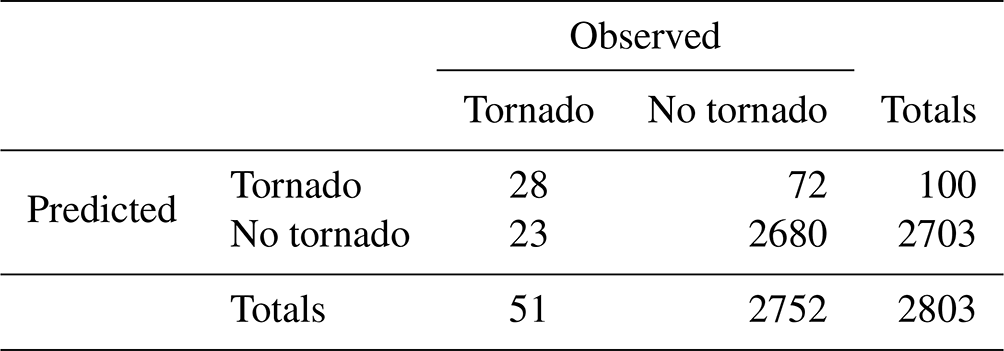
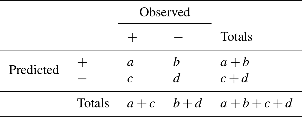
From the totals in the bottom row, we find that the base rate – the climatological probability, as it is sometimes called – of tornado occurrence is a little under 2 %, i.e. 51 observations of tornadoes against 2752 observations of non-tornadoes, well below the 5 % base rate used to classify rare and severe event forecasting (Murphy, 1991). Further, combining the figures of the top left and bottom right entries, we obtain the total number of verified predictions (of both occurrence and of non-occurrence) in the 3-month period. Out of a total of 2803 predictions, 2708 were correct, which is an impressive success rate of over 96 %. This figure goes by many names: among the more common, it is known as the percentage correct (when multiplied by 100), the proportion correct, the hit rate or simply accuracy. In a table laid out as in Table 2 – commonly referred to as a 2×2 contingency table or confusion matrix – it is the proportion $\frac{a+d}{a+b+c+d}$, which gives us the proportion of predictions that are successful or “verified”.

Table 2 Standard characterization of a 2×2 contingency table.

The questions we focus on are (1) what this type of accuracy tells us about forecast performance or forecasting skill in the case of rare event forecasting and (2) how best to measure and compare different RSE forecast performances.

2.2 The accuracy paradox: accuracy vs. skill

A feature of tornadoes and also of snow avalanches is that they are rare events, that is $a+c\ll b+d$. As a result, a forecaster will exhibit high accuracy or attain a high proportion correct simply by predicting “no tornado” or “no avalanche” all the time. This trivial (but often overlooked) observation is nowadays blessed with the name the accuracy paradox (e.g. Bruckhaus, 2007; Thomas and Balakrishnan, 2008; Fernandes, 2010; Brownlee, 2014, 2020; Valverde-Albacete and Peláez-Moreno, 2014; Akosa, 2017; Uddin, 2019; Davis and Maiden, 2021). The point at issue was made robustly in a letter to the editor in the 15 August 1884 issue of Science, a correspondent named only as “G.” writing “An ignoramus in tornado studies can predict no tornadoes for a whole season, and obtain an average of fully ninety-five per cent” (G., 1884).

Indeed, as Finley makes more incorrect predictions of tornadoes (72) than correct ones (28) (b>a in Table 2), it was quickly pointed out that he would have done better by his own lights if he had uniformly predicted no tornado (Gilbert, 1884) – he would then have caught up with the skill-less ignoramus whose accuracy, all else equal, would have been an even more impressive 98.2 % ($\frac{b+d}{a+b+c+d}$ in Table 2). Where the prediction of rare events is concerned, this strongly suggests that accuracy, the proportion correct, is not an appropriate measure of the skill involved. While we argue for this in more detail in the next section, two concerns counting against accuracy can be noted immediately.

First, focusing on accuracy in rare event forecasting often rewards skill-less performances and incentivizes “no-occurrence” predictions. Second, where the prediction of severe events is concerned, such an incentive is hugely troubling as a failure to predict occurrence is usually far more serious than an unfulfilled prediction of occurrence. As Allan Murphy observes,

Since it is widely perceived that type 2 errors [failures to predict occurrences, c in Table 2] are more serious than type 1 errors [unfulfilled predictions of occurrence, b in Table 2], forecasts of RSEs generally are characterized by overforecasting. That is, over a set of forecasting occasions, more RSEs are usually forecast to occur than are subsequently observed to occur [i.e, in terms of Table 2, $a+b>a+c$]. (Murphy, 1991)

The accuracy measure is, then, doubly unsuitable when it comes to assessing the skill involved in RSE forecasting.

But if not by accuracy, how should we assess the quality of a set of RSE forecasts? Immediately after the publication of Finley's article, a number of US government employees rose to the challenge. In the next section, we outline the skill measures they introduced, and in doing so we motivate three adequacy constraints that skill measures in RSE forecasting ought to meet.

3 What is skill? Three adequacy constraints on skill measures for RSE forecasting

3.1 First adequacy constraint: better than chance

Gilbert (1884) responded immediately to Finley's article and in doing so made two lasting contributions to forecast verification. His thought was straightforward. Anybody making a sequence of forecasts, whether skilled or unskilled, is likely to get some right by chance. How many? In Table 2, there are a+c occurrences of tornadoes in the sequence of $a+b+c+d$ forecasting occasions. The forecaster makes a+b forecasts of occurrence. If these a+b forecasts were made “randomly” – by “random prognostication” as Gilbert called it – we should expect a fraction $\frac{a+c}{a+b+c+d}$ of them to be correct. So the “number”, a_r, of predictions of occurrence that we might expect the skill-less forecaster to get right by luck or chance is $\frac{a+c}{a+b+c+d}\times (a+b)$, i.e. the number in proportion to the base rate. Likewise, in parallel fashion, we work out the “number”, d_r, of predictions of non-occurrence we might expect the skill-less forecaster to get right by chance; the “number”, b_r, of predictions of occurrence we might expect the skill-less forecaster to get wrong by chance; and the “number”, c_r, of predictions of non-occurrence we might expect the skill-less forecaster to get wrong by chance keeping fixed the marginal totals a+b, c+d, a+c and b+d. We find

$$\begin{array}{}\text{(1)}& \begin{array}{rl}& a_{\mathrm{r}}={\displaystyle \frac{(a+b)(a+c)}{a+b+c+d}},b_{\mathrm{r}}={\displaystyle \frac{(a+b)(b+d)}{a+b+c+d}},\\ & c_{\mathrm{r}}={\displaystyle \frac{(a+c)(c+d)}{a+b+c+d}},d_{\mathrm{r}}={\displaystyle \frac{(b+d)(c+d)}{a+b+c+d}}.\end{array}\end{array}$$

(We put “number” in scare quotes because $\frac{(a+c)(a+b)}{a+b+c+d}$ need not take a whole number value. It is a familiar fact that an expected value need not be a realizable value – no undamaged face on a fair die has three and a half spots on it.)

a−a_r is then the number of successful predictions of occurrence that we credit to the forecaster's skill, and d−d_r is the number of successful predictions of non-occurrence. As Gilbert noted,

$$\begin{array}{}\text{(2)}& a-a_{\mathrm{r}}=d-d_{\mathrm{r}}={\displaystyle \frac{ad-bc}{a+b+c+d}}.\end{array}$$

The forecaster does better than chance if a>a_r, equivalently, if d>d_r, i.e. if ad>bc. (For a rigorous derivation of a_r, see Appendix A.)

It is also the case that

$$\begin{array}{}\text{(3)}& b_{\mathrm{r}}-b=c_{\mathrm{r}}-c={\displaystyle \frac{ad-bc}{a+b+c+d}}.\end{array}$$

What do b_r−b and c_r−c represent? When the forecaster does better than chance, they are the improvements over chance, thus decreases in, respectively, the making of Type I and the making of Type II errors.

Given these considerations, we can now substantiate our earlier claim that Finley exhibited genuine skill, in contrast to the ignoramus, in issuing his predictions. While Finley's 28 correct out of 100 predictions of occurrence made may not seem impressive, his score is a fraction over 15 times more than he could have expected to get right by chance, given Table 1's numbers – Finley's performance was skilful.

That was Gilbert's first contribution. Although the next step we take is not exactly Gilbert's, the idea behind it is his second lasting contribution. Our forecaster makes $a+b+c+d$ predictions. How many do we credit to their skill? Gilbert's suggestion is $(a-a_{\mathrm{r}})+b+c+(d-d_{\mathrm{r}})$, a suggestion in effect taken up by Glenn Brier and R. A. Allen (1951) when they give this general form for a skill score:

$$\begin{array}{}\text{(4)}& {\displaystyle \frac{\mathrm{actual}\mathrm{score}-\mathrm{score}\mathrm{attainable}\mathrm{by}\mathrm{chance}}{\mathrm{total}\mathrm{number}\mathrm{of}\mathrm{forecasts}-\mathrm{score}\mathrm{attainable}\mathrm{by}\mathrm{chance}}}.\end{array}$$

Here, in both numerator and denominator, the score attainable by chance is a_r+d_r. So, instead of accuracy's $\frac{\mathrm{successes}}{\mathrm{predictions}}$ as a measure that does not take into account skill, we take

$$\begin{array}{}\text{(5)}& \begin{array}{rl}& {\displaystyle \frac{\mathrm{successes}\mathrm{owed}\mathrm{to}\mathrm{skill}}{\mathrm{predictions}\mathrm{credited}\mathrm{to}\mathrm{skill}}},\mathrm{i}.\mathrm{e}.\\ & {\displaystyle \frac{\left(a-a_{\mathrm{r}}\right)+\left(d-d_{\mathrm{r}}\right)}{\left(a-a_{\mathrm{r}}\right)+b+c+\left(d-d_{\mathrm{r}}\right)}}.\end{array}\end{array}$$

This is

$$\begin{array}{}\text{(6)}& {\displaystyle \frac{\mathrm{2}(ad-bc)}{(a+b)(b+d)+(a+c)(c+d)}}.\end{array}$$

This is a skill score that, in contrast to accuracy, meets our first adequacy constraint as it controls for chance and aims at genuinely skilful predictions. In the forecasting literature, this measure is known as the special case of the Heidke skill score (Heidke, 1926) applicable to binary categorical forecasting. It was first mentioned by M. H. Doolittle (1888), but he dismissed it as not having any scientific value. (As we explain below, we have some sympathy with Doolittle's judgement.)

We can rewrite the Heidke skill score as

$$\begin{array}{}\text{(7)}& {\displaystyle \frac{\left(b_{\mathrm{r}}-b\right)+\left(c_{\mathrm{r}}-c\right)}{b_{\mathrm{r}}+c_{\mathrm{r}}}}.\end{array}$$

The score is then revealed to be the proportional improvement (decrease) over chance in the making of errors of both Type I and Type II (and if one says only this about it, we have no complaint to make).

Now, if we take it that the best a forecaster can do is have all their predictions, of both occurrence and non-occurrence, fulfilled then, following Woodcock (1976), we can present the Heidke skill score in an interestingly different way:

$$\begin{array}{}\text{(8)}& {\displaystyle \frac{\mathrm{actual}\mathrm{score}-\mathrm{score}\mathrm{attainable}\mathrm{by}\mathrm{chance}}{\mathrm{best}\mathrm{possible}\mathrm{score}-\mathrm{score}\mathrm{attainable}\mathrm{by}\mathrm{chance}}}.\end{array}$$

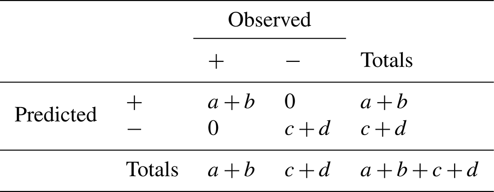
Here, as said, we equate the “best possible score” with correctly predicting all occurrences and non-occurrences – a+c correct predictions of occurrence and b+d correct predictions of non-occurrence (Table 3). Substituting into the above equation, we obtain the Heidke skill score, for the actual score, the actual number of successful predictions is a+d, the number attributable to chance is a_r+d_r and the best possible score is $a+b+c+d$.

Table 3 Best possible score relative to Table 2's data on occurrence.

Focusing on the notion of a best possible score, though, gives us a different way to think about skill. On the model of what we did above, someone randomly making a+c predictions of occurrence could expect to get $\frac{(a+c)(a+c)}{a+b+c+d}$ of them right by chance, and, likewise, someone randomly making b+d forecasts of non-occurrence could expect to get $\frac{(b+d)(b+d)}{a+b+c+d}$ of them right by chance. So in the case of perfect prediction, in which there are no Type I or Type II errors, the number of successes we credit to the forecaster's skill is

$$\begin{array}{}\text{(9)}& (a+b+c+d)-{\displaystyle \frac{(a+c{)}^{\mathrm{2}}+(b+d{)}^{\mathrm{2}}}{a+b+c+d}}={\displaystyle \frac{\mathrm{2}(a+c)(b+d)}{a+b+c+d}}.\end{array}$$

Putting a different reading on our rewriting of Brier and Allen's conception of a skill score, namely

$$\begin{array}{}\text{(10)}& {\displaystyle \frac{\mathrm{actual}\mathrm{score}-\mathrm{score}\mathrm{attainable}\mathrm{by}\mathrm{chance}\left(\mathrm{relative}\mathrm{to}\mathrm{actual}\mathrm{performance}\right)}{\mathrm{best}\mathrm{possible}\mathrm{score}-\mathrm{score}\mathrm{attainable}\mathrm{by}\mathrm{chance}\left(\mathrm{relative}\mathrm{to}\mathrm{best}\mathrm{possible}\mathrm{performance}\right)}},\end{array}$$

we get

$$\begin{array}{}\text{(11)}& {\displaystyle \frac{\mathrm{2}(ad-bc)}{\mathrm{2}(a+c)(b+d)}}={\displaystyle \frac{a}{a+c}}-{\displaystyle \frac{b}{b+d}},\end{array}$$

which is known as the Peirce skill score (Peirce, 1884), the Kuipers skill score (KSS; Hanssen and Kuipers, 1965) and the true skill statistic (TSS; Flueck, 1987). (Peirce's own way of arriving at the Peirce skill score is quite different, which is examined in detail in Milne, 2021.)

We can think of the Peirce skill score as being this ratio:

$$\begin{array}{}\text{(12)}& {\displaystyle \frac{\mathrm{successes}\mathrm{due}\mathrm{to}\mathrm{skill}\mathrm{in}\mathrm{actual}\mathrm{performance}}{\mathrm{successes}\mathrm{due}\mathrm{to}\mathrm{skill}\mathrm{in}\mathrm{perfect}\mathrm{performance}}},\end{array}$$

and we will discuss this way of thinking of the Peirce skill score further in what follows.

To summarize, one of the earliest responses to the challenge to identify the skill involved in RSE forecasting was to highlight the need to take into account, in some way, the possibility of getting predictions right “by chance” and thus present the skill exhibited in a sequence of forecasts as relativized to what a “random prognosticator” could get right by chance. As we have just seen, this can be done in different ways which motivate different measures of skill. At this point, we do not have much to say on whether Gilbert's and Brier and Allen's reading or our rewrite is preferable, i.e. whether the Heidke or Peirce skill score is preferable. However, we can note that this first adequacy constraint rules out simple scores such as accuracy (proportion correct) as capturing anything worth calling skill in forecasting.

We should note that some measures in the literature, in particular those that are functions of a, b and c only, such as the $\frac{a}{a+b+c}$ of Gilbert (1884); the Dice coefficient $\frac{\mathrm{2}a}{\mathrm{2}a+b+c}$, also called the F score or F₁, and its generalization, the adjusted F measure, $F_{\mathit{\beta }}=\frac{(\mathrm{1}+{\mathit{\beta }}^{\mathrm{2}})a}{(\mathrm{1}+{\mathit{\beta }}^{\mathrm{2}})a+b+{\mathit{\beta }}^{\mathrm{2}}c}$; and $\frac{a}{\sqrt{(a+b)(a+c)}}$, sometimes called the Fowlkes–Mallows index or the cosine similarity, do not build in a correction for chance successes. The measures just mentioned are expressible as functions of $\frac{a}{a+b}$ (the frequency of hits, FOH) and $\frac{a}{a+c}$ (the probability of detection, POD, or hit rate), as Gilbert (1884) initially proposed any measure of forecasting quality should be; he tacitly gave up on that commitment when he hit upon the idea of discounting the number of successful predictions attainable by chance. Now, we can evaluate these measures setting a, b and c to the values they take for random prognostication, i.e. a_r, b_r and c_r (which are all functions of a, b, c and d). When we do this we find that each of the measures returns a value greater than it yields for random prognostication when, and only when, ad>bc. The argument is straightforward: except at the extremes, i.e. except when a>0 and $b=c=\mathrm{0}$, when each of these measures takes the value 1, or when a=0 and $b+c>\mathrm{0}$ (or $b\times c>\mathrm{0}$ in the case of the Fowlkes–Mallow coefficient), when each of the measures takes the value 0, each of the measures is strictly increasing in a and strictly decreasing in b and in c; as we saw above, a>a_r if, and only if, b_r>b if, and only if, c_r>c if, and only, if ad>bc. Hence each counts a performance as better than chance (random prognostication) if, and only if, ad>bc. All well and good but a significant weakness of these measures looms exactly here, namely that what value each assigns random prognostication is highly context dependent – dependent on the values of a, b, c and d so that the same value of the measure may on one occasion indicate a better-than-chance performance and on another a worse-than-chance performance. With these measures, then, whether a performance is better than chance and to what extent has to be worked out on a case-by-case basis, a significant demerit.

Satisfaction, or not, of the criterion that ad>bc, depends, of course, on there being a value for d. Jolliffe (2016) picks up on this when, while acknowledging that the Dice and Gilbert measures just considered “have undesirable properties”, he says that “the Dice coefficient is of use when the number of `correct rejections', d, is unknown, is difficult to define or is so large that it dominates the calculation of most measures” (p. 89). The first two render assessment of whether a performance is better than chance at best doubtful and at worst impossible; the third renders it trivial (assuming a≠0). We take the implication of Jolliffe's remarks to be that measures such as Gilbert's original – the Jaccard coefficient as it is often called, Dice's and the cosine similarity are only of use when, for whatever reason, the number of successful predictions of non-occurrence is either not well defined or not known, which however is usually not the case for RSE forecasting.

3.2 Second adequacy constraint: direction of fit

Doolittle (1885a, b) introduced a measure of “that part of the success in prediction which is due to skill and not to chance” that is the product of two measures now each better known in the forecasting literature than Doolittle's own, the Peirce skill score, which we have just introduced, expressed in terms of Table 2 as $\frac{a}{a+c}-\frac{b}{b+d}$, and the Clayton skill score (Clayton, 1927, 1934, 1941), expressed in the same terms as $\frac{a}{a+b}-\frac{c}{c+d}$. Even before publication, Doolittle was criticized by Henry Farquhar (1884): Doolittle had, said Farquhar, combined a measure that tests occurrences for successful prediction (the Peirce skill score) with a measure that tests predictions for fulfilment (the Clayton skill score). Now, Doolittle's measure is indeed the product of the indicated measures, and Farquhar is correct in his claim regarding what those measures measure. But why is this ground for complaint? Doolittle saw none. Apparently taking on board Farquhar's observation, he says

Prof. C. S. Peirce (in Science. Nov. 14, 1884, Vol. IV., p. 453), deduces the value $i=\frac{a(a+b+c+d)-(a+c)(a+b)}{(a+c)(b+d)}\left[=\frac{a}{a+c}-\frac{b}{b+d}\right]$, by a method which refers principally to the proportion of occurrences predicted, and attaches very little importance to the proportion of predictions fulfilled. (Doolittle, 1885b, p. 328, with a change of notation)

Farquhar allows that “either of these differences [i.e. the Peirce skill score and the Clayton skill score] may be taken alone, with perfect propriety”. By multiplying the Peirce skill score and the Clayton skill score, one is multiplying a measure that tests occurrences for successful prediction by a measure that tests predictions for fulfilment. The resulting quantity is neither of these things – but that, in itself, does not formally prevent it being, as Doolittle took it to be, a measure of the skill exhibited in prediction. Why, then, should one not multiply them, or put differently what is wrong with Doolittle's measure?

The answer, we suggest, lies in a notion known to philosophers as direction of fit. The idea, but not the term, is usually credited to Elizabeth Anscombe, who introduced it as follows.

Let us consider a man going round a town with a shopping list in his hand. Now it is clear that the relation of this list to the things he actually buys is one and the same whether his wife gave him the list or it is his own list; and that there is a different relation where a list is made by a detective following him about. If he made the list itself, it was an expression of intention; if his wife gave it him, it has the role of an order. What then is the identical relation to what happens, in the order and the intention, which is not shared by the record? It is precisely this: if the list and the things that the man actually buys do not agree, and if this and this alone constitutes a mistake, then the mistake is not in the list but in the man's performance (if his wife were to say “Look, it says butter and you have bought margarine”, he would hardly reply “What a mistake! we must put that right” and alter the word on the list to “margarine”); whereas if the detective's record and what the man actually buys do not agree, then the mistake is in the record. (Anscombe, 1963, Sect. 32)

As Anscombe's observation regarding butter and margarine makes clear, the ideal performance for the husband is to have the contents of his shopping basket match his shopping list; the ideal performance for the detective is for his list to match the contents of the shopping basket. The difference lies in whether list or basket sets the standard against which the other is evaluated – this is the difference in direction of fit. Put bluntly, Peirce has the sequence of weather events set the standard and evaluates sequences of predictions against that standard; Clayton has the sequence of actual predictions set the standard and evaluates sequences of weather events against that standard. This difference in direction of fit is beautifully pointed out by Doolittle himself. Contrasting Peirce's measure with the other component of his own, the Clayton skill score as we now know it, he says

Prof. C. S. Peirce (in Science, Nov. 14, 1884, Vol. IV., p. 453), deduces the first of these factors as the unqualified value of i [the inference-ratio or that part of the success which is due to skill and not to chance] …. He obtains his result by the aid of the supposition that part of the predictions are made by an infallible prophet, and the others by a man ignorant of the future. If Prof. Peirce had called on omnipotence instead of omniscience, and supposed the predictions to have been obtained from a Djinn careful to fulfill a portion of them corresponding to the data, the remainder of the occurrences being produced by an unknown Djinn at random, he would have obtained by parallel reasoning the second factor. (Doolittle, 1885a, p. 124)

When measuring occurrences for successful prediction, the aim is to match predictions to the world, something which an omniscient being succeeds in doing; in measuring predictions for fulfilment, the ideal is to have the world match the predictions made, something which an omnipotent being can arrange to be the case.

In considering improvements on the forecasting performance recorded in Table 2, what are kept fixed are the numbers of actual occurrences and non-occurrences, the marginal totals a+c and b+d, not the numbers of actual predictions of occurrence and predictions of non-occurrence, the marginal totals a+b and c+d. It is, after all, only a poor joke to say “I would have had a higher skill score if more tornadoes had occurred”, even though it may well be true. Doolittle has, despite himself, made clear for us that forecasters are like Anscombe's detective and not like the husband with the shopping list. Forecasters aim to fit their predictions to the world, not the world to their predictions.

Let us go back to this form for a skill score:

$$\begin{array}{}\text{(13)}& {\displaystyle \frac{\mathrm{actual}\mathrm{score}-\mathrm{score}\mathrm{attainable}\mathrm{by}\mathrm{chance}\left(\mathrm{relative}\mathrm{to}\mathrm{actual}\mathrm{performance}\right)}{\mathrm{best}\mathrm{possible}\mathrm{score}-\mathrm{score}\mathrm{attainable}\mathrm{by}\mathrm{chance}\left(\mathrm{relative}\mathrm{to}\mathrm{best}\mathrm{possible}\mathrm{performance}\right)}}.\end{array}$$

Peirce's conception of the best possible performance, presented above in Table 3, keeps the marginal totals for actual observed occurrences and non-occurrences from Table 2, a+c and b+d, respectively. The actual numbers of occurrence and non-occurrence set the standard against which performances are measured; thus constrained, the best possible performance is that of the as-it-were omniscient being who correctly predicts all occurrences and all non-occurrences (Table 3).

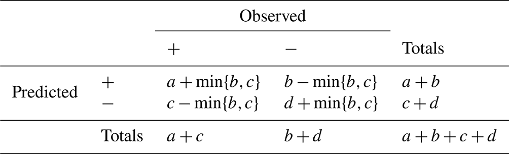
Clayton's conception of the best possible performance, presented in Table 4, keeps the marginal totals for actual predictions of occurrence and predictions of non-occurrence from Table 2, a+b and c+d, respectively. The actual numbers of predictions of occurrence and predictions of non-occurrence provide the standard against which performances are measured; thus constrained, the best possible performance is that of the omnipotent being who fashions occurrences and non-occurrences to fit their predictions (Table 4). And so, returning to our original question, it should now be clear what is wrong with Doolittle's measure: it incorporates Clayton's measure, which has the wrong direction of fit for a measure of skill in prediction.

Table 4 Omnipotent forecaster's score relative to Table 2's data on prediction.

What of the Heidke skill score? How does it fare with respect to direction of fit? What conception of best performance does it employ? In its denominator, the Heidke score takes the best possible performance to be one in which all $a+b+c+d$ predictions are correct but corrects that number for chance using Table 2's marginal totals for both predictions and occurrences. This is, quite simply, incoherent – unless, fortuitously, we are in the special case when the numbers of Type I and Type II errors are equal. Keeping Table 2's marginal totals, the highest attainable number of correct predictions is $a+d+\mathrm{2}\times \min \mathit{\{}b,c\mathit{\}}$ (Table 5), not $a+b+c+d$.

Table 5 Highest number of correct predictions relative to Table 2's marginal totals.

Using the marginal totals in Table 5, which are, by design, those of Table 2, to correct $a+d+\mathrm{2}\times \min \mathit{\{}b,c\mathit{\}}$ for chance, we obtain this skill score:

$$\begin{array}{}\text{(14)}& {\displaystyle \frac{ad-bc}{(a+\min \mathit{\{}b,c\mathit{\left\}}\right)\left(\min \mathit{\right\{}b,c\mathit{\}}+d)}}.\end{array}$$

This measure, which had previously occurred in other literature (Benini, 1901; Forbes, 1925; Johnson, 1945; Cole, 1949), has been used to assess forecasting performances not in tornado forecasting or in avalanche forecasting but in assessing predictions of juvenile delinquency and the like in criminology where it is known as RIOC, relative improvement over chance (Loeber and Dishion, 1983; Loeber and Stouthamer-Loeber, 1986; Farrington, 1987; Farrington and Loeber, 1989; Copas and Loeber, 1990).

The RIOC measure has the following feature: when there are successes in predicting occurrences and non-occurrence, i.e. a>0 and d>0, it awards a maximum score of 1 to any forecasting performance in which there are either no Type I errors (b=0) or no Type II errors (c=0) or both. This is a feature it shares with the odds ratio skill score (ORSS) of Stephenson (2000) (see Appendix D). In agreement with Woodcock (1976), we hold that a maximal score should be attained when, and only when, b and c are both zero.

That is one problem with the RIOC measure. The other is this. Like Anscombe's detective, the scientific forecaster's aim is to match their predictions to what actually happens. This is why we keep the column totals fixed when considering the best possible performance. Why on earth should we also keep the row totals and the numbers of predictions of occurrence and non-occurrence fixed? There is, we submit, no good reason to do so. The Heidke skill score embodies no coherent conception of best possible performance. The RIOC of Loeber et al. does at least embody a coherent notion of best possible performance, but it is a needlessly hamstrung one, restricting the range of possible performances to those that make the same number of predictions of occurrence and of non-occurrence as the actual performance. On the one hand, this makes a best possible performance too easy to achieve and, on the other, sets our sights so low as to only compare a forecaster with others who make the same number of forecasts of occurrence and of non-occurrence – but forecasting is a scientific activity, not a handicap sport.

Finally, for completeness, let us consider the measure we started out with, proportion correct, $\frac{a+d}{a+b+c+d}$. How does it fare with respect to the second adequacy constraint? While it may be true to say that it does not evaluate a performance in relation to the wrong direction of fit, this is the case only because the measure does not properly engage with the issue of fit. Here, the evaluation is in relation to $a+b+c+d$, and so the performance is not evaluated in relation to any relevant proportion (either of occurrences or of predictions). A similar consideration applies to Gilbert's original measure $\frac{a}{a+b+c}$. More generally, though, the measures we considered at the end of the previous section, Gilbert's original, F₁/the Dice coefficient and the adjusted F measures, the F_β family, and the Fowlkes–Mallows index/cosine similarity, are, as we said, functions of $\frac{a}{a+b}$ and $\frac{a}{a+c}$. Uncorrected for chance though they be, these are, as Farquhar put it, a measure that tests predictions for fulfilment and a measure that tests occurrences for successful prediction, respectively. Our complaint against these measures is, then, the same as our complaint against Doolittle's measure: each incorporates a component which has the wrong direction of fit for a measure of skill in prediction.

The notion of direction of fit has much wider application than just forecasting: it applies in any setting in which we can see “the world” or a “gold standard test” or, more prosaically, some aspect of the set-up in question as setting the standard against which a “performance” is judged. Diagnostic testing is one obvious case – and there we have the Peirce skill score but under the name of the Youden index (Youden's J) (Youden, 1950); in medical/epidemiological terms, it is commonly expressed as $\mathrm{sensitivity}+\mathrm{specificity}-\mathrm{1}$. More widely used to summarize diagnostic accuracy is the (positive) likelihood ratio $\frac{\mathrm{sensitivity}}{\mathrm{1}-\mathrm{specificity}}$ (Deeks and Altman, 2004; Šimundić, 2009/2012b), but this is a function of the same proportions and so fares equally well in terms of direction of fit. By way of contrast, in information retrieval, following the lead of early work by M. Lesk and G. Salton (1969), M. H. Heine (1973), and N. Jardine and C. J. van Rijsbergen (1971; see also van Rijsbergen, 1974), it has become common practice to measure the effectiveness of a retrieval system in terms of precision, i.e. proportion of retrieved items that are relevant, and recall, i.e. the proportion of relevant items retrieved, committing exactly the direction-of-fit error we have diagnosed in the applications of the Doolittle, Gilbert, Dice, F_β and cosine similarity measures with “relevant” playing the role of “observed” and “retrieved” that of “predicted” in Table 2. (It should be noted that the analogue of the Peirce skill score, known as recall−fallout, has had its advocates in information retrieval – see Goffman and Newill, 1966; Robertson, 1969a, b – but in practice the F measures, and F₁ in particular, have come to dominate, so much so that “it is now virtually impossible to publish work in information retrieval or natural language processing without including it [F₁]” Powers, 2015/2019.)

So, in summary, we can say that in any context in which direction of fit plays a role, the Peirce score, alone of scores in the literature, evaluates performances in relation to the correct proportions (occurrences and non-occurrences predicted).

3.3 Third adequacy constraint: weighting errors

We think there is a third feature of skill that is specific to severe event forecasting that a skill measure ought to take into account. Broadly speaking, it consists in being sensitive, in the right kind of way, to one's own fallibility. While the omniscient forecaster need not worry about mistakes, actual forecasters need to be aware of the different kinds of consequences of an imperfect forecast. To motivate our third constraint, consider the two forecasts in Table 6.

Table 6 Example of two forecasts (A, B) that agree on the correct predictions and the total number of false predictions but differ in the kinds of false predictions (Type I vs. Type II).

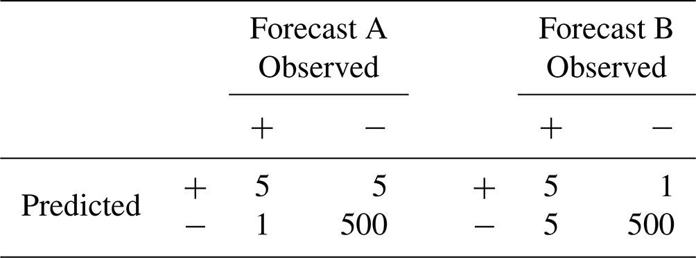
While forecasts A and B issue the same total number of forecasts and both score an excellent 98.8 % accuracy, they disagree on the kinds of errors they make. Forecast A makes fewer Type II errors (1) than Type I errors (5), while in forecast B this error distribution is reversed. Is there a reason to think that one forecast is more skilful than the other?

Given the context of our discussion, i.e. rare and severe event forecasting, we believe there is. We saw Allan Murphy saying that “it is widely perceived that type 2 errors [erroneous predictions of non-occurrence] are more serious than type 1 errors [unfulfilled predictions of occurrence]”. A skilful RSE forecaster should take this observation into account and consider, as it were, the effects of their mistakes. As a result a skill measure should incorporate – in a principled way – the different effects of Type I and Type II errors and judge forecast A as more skilful than forecast B, at least when the forecast is evaluated in the context of RSE forecasting.

Importantly, the Peirce skill score does just that. We can re-write it as

$$\begin{array}{}\text{(15)}& \mathrm{1}-{\displaystyle \frac{c}{a+c}}-{\displaystyle \frac{b}{b+d}}\end{array}$$

and read it as making a deduction from 1, the score for a perfect omniscient performance, for each Type II and each Type I error. Now, when we are concerned with rare events, i.e. when $a+c\ll b+d$, the “deduction per unit” is greater for Type II errors than for Type I errors. As a result, it is built into the Peirce skill score, in a principled way, that Type II errors count for more than Type I errors when we are dealing with rare events. This is borne out in the Peirce skill score for our two forecasts above: forecast A receives a score of 0.823 while forecast B receives a score of 0.498. Note that this feature of the Peirce score would turn into a liability if we were to consider very common but nevertheless severe events. (Put contrapositively, the Peirce skill score increases the relative score of correct predictions of occurrence as the base rate of occurrences decreases; Gandin and Murphy, 1992; Manzato, 2005.)

Now, when d is large, as it often is in the case of rare event forecasts, it is likely to be the case that $a+b\ll c+d$. When this is the case the Clayton skill score, which we may write as

$$\begin{array}{}\text{(16)}& \mathrm{1}-{\displaystyle \frac{b}{a+b}}-{\displaystyle \frac{c}{c+d}},\end{array}$$

turns the good behaviour of the Peirce skill score on its head, giving a greater deduction per unit for Type I errors than for Type II errors. According to the Clayton skill score, we should regard forecast B (0.823) as more skilful than forecast A (0.498). So, not only does the Clayton skill score fail to meet the direction of fit requirement, it also fails – in quite a spectacular way – our third requirement of weighting errors.

Formally, the Heidke skill score treats Type I and Type II errors equally in that interchanging b and c, i.e. Type I and Type II errors, in

$$\begin{array}{}\text{(17)}& {\displaystyle \frac{\mathrm{2}(ad-bc)}{(a+b)(b+d)+(a+c)(c+d)}}\end{array}$$

leaves the measure unchanged. To wit, according to the Heidke skill score, forecasts A and B are equally skilful with a measure of 0.619.

In fact all measures known to us in the forecasting literature other than the Peirce skill score, the Clayton skill score and the F_β measure (which places more weight on minimizing Type II errors when β>1) behave like the Heidke skill score on this issue: interchanging b and c leaves the measure unchanged, and Type I and Type II errors are on a par (see Appendix D for a list of other skill scores for each of which this claim can easily be confirmed). Nonetheless, we can say in favour of the Heidke score that it provides the right incentive: in an application in which $b+d>a+c$, as it is in the case of rare event forecasting, an increase in Type II errors would lower the actually attained score by more than the same number of Type I errors, and a decrease in Type II errors would increase the actually attained score by more than the same number fewer Type I errors (see Appendix B for the formal details).

Table 7 collates our main claims and presents each of the measures discussed so far in relation to the three adequacy constraints. It is worth noting that while the first requirement arises in particular in the case of rare event forecasting, both the first and second are, arguably, relevant also in common event forecasting. The third constraint, however, is distinctive of severe event forecasting.

Table 7 Summary comparison of skill measures in relation to the three adequacy constraints for RSE forecasting.

Finally, should we consider these three constraints as jointly sufficient? Of course, further debate may generate other adequacy constraints on skill measures, and we are open to such a development at this stage of the discussion. However, we take ourselves to have shown that there really is only one skill measure in the forecasting literature that meets the three constraints, and so there is only one genuine candidate for a measure of skill in RSE forecasting.

4 Application: the relevance of skill scores in avalanche forecast verification

In this section, we will show how our theoretical discussion concerning skill measures has consequences for the practice of avalanche forecast verification. We focus on the use of the nearest-neighbour (NN) method of avalanche forecasting as discussed in Heierli et al. (2004). The idea of NN forecasting for avalanches dates back to the 1980s (Buser, 1983, 1989; Buser et al., 1987) and has been widely used for avalanche forecasting in Canada, Switzerland, Scotland, India, and the US (e.g. McClung and Tweedy, 1994; Cordy et al., 2000; Brabec and Meister, 2001; Gassner et al., 2001; Gassner and Brabec, 2002; Purves et al., 2003; Heierli et al., 2004; Roeger et al., 2004; Singh and Ganju, 2004; Zeidler and Jamieson, 2004; Singh et al., 2005; Purves and Heierli, 2006; Singh et al., 2015). To evaluate the quality of this forecasting technique, forecast verification is an indispensable tool, and this process can take on different forms (Purves and Heierli, 2006). In the case of binary NN forecasts, a variety of measures have been used in the verification process, though there is currently no consensus about how to adjudicate between them (Heierli et al., 2004). Most studies simply present a list of different measures without providing principled reasons as to which measure is the most relevant one (an exception is Singh et al., 2015, who opt for the Heidke score). This section offers a discussion as to how the many different measures should be used and ranked in their relevance for avalanche forecast verification in the context of binary NN forecasting. It is worth noting, however, that broadly similar considerations will be applicable to the verification used in other avalanche forecasting techniques, or indeed to other kinds of binary RSE forecasts and their verification, such as landslides (e.g. Leonarduzzi and Molnar, 2020; Hirschberg et al., 2021).

The basic assumption of the NN forecasting approach is that similar conditions, such as the snowpack, temperature, weather, etc., will likely lead to similar outcomes, and so historical data – weighted by relevance and ordered by similarity – are used to inform forecasting. More specifically, NN forecasting is a non-parametric pattern classification technique where data are arranged in a multi-dimensional space and a distance measure (usually the Brier score) is used to identify the most similar neighbours. NN forecasting can be used for categorical or probabilistic forecasts. In the case of the former, which is relevant to our current discussion, a decision boundary k is set and an avalanche is forecast; i.e. a positive prediction is issued, when the number of positive neighbours (i.e. nearest neighbours on which an avalanche was recorded) is greater than or equal to that decision boundary k.

The study of Heierli et al. (2004) on avalanche forecast verification uses two datasets, one focused on Switzerland and the other on Scotland. Figure 1 summarizes their results and nicely shows how changes in the decision boundary k affect a variety of measures, such as accuracy and other skill measures. In what follows, we will follow their lead and investigate their finding through a more “methodological” lens. Using their study will help us explain differences in behaviour of the skill measures given variations in the decision boundary and highlight how our discussion has practical consequences. As Heierli et al. (2004) emphasize, one core issue for NN forecasting is which decision boundary k should be chosen, i.e. for which k do we get the “best” forecast. Naturally, this choice should depend, crucially, on how we assess the goodness of the different forecasts given variations in k. Our proposal is that the choice of k should be settled by establishing which value of k issues the most skilful forecast. We should note that manipulating the value of k in NN forecasting is a special case of using different values of a parameter to categorize items – future events, say – in two classes. One can plot $\frac{a}{a+c}$, which, in the case of forecasting, is the probability of detection, against $\frac{b}{b+d}$, the probability of false detection, as it is sometimes called, resulting from different values of the parameter, to yield a receiver operating characteristic (ROC) curve (Swets, 1973; Metz, 1978; Altman and Bland, 1994; Šimundić, 2009/2012a; Manzato, 2005, 2007). The Peirce skill score at a point on the curve, $\frac{a}{a+c}-\frac{b}{b+d}$, is a measure of the distance of the point from the line x=y, which represents a forecast of zero value. It seems built into this approach that the Peirce skill score is a measure of forecast quality.

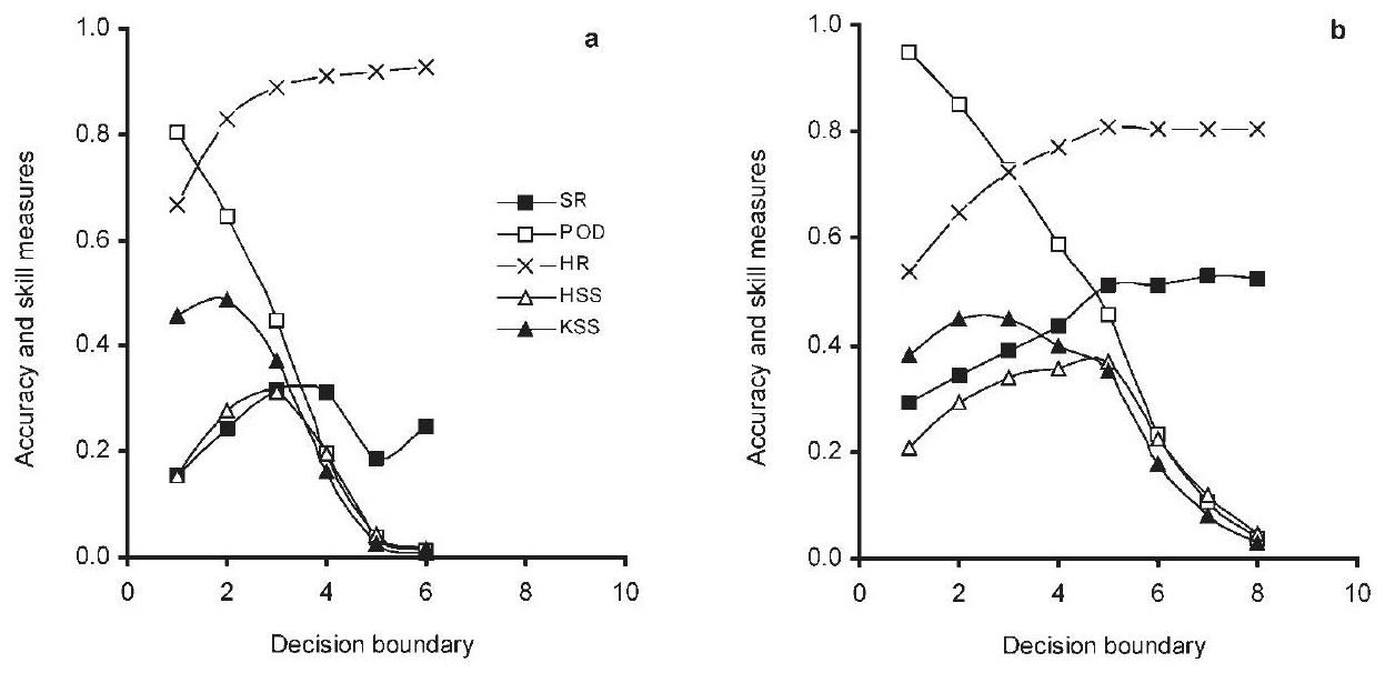
Figure 1 Dependence of accuracy and skill measures on the choice of decision boundary (number of positive neighbours of the forecast day). (a) Swiss dataset; (b) Scottish dataset. From Heierli et al. (2004) and reprinted from the Annals of Glaciology with permission of the International Glaciological Society and the lead author.

Let us start our discussion by noting two immediate consequences of NN avalanche forecasting. Remember that a positive prediction is issued when the number of positive neighbours is equal to or greater than k. From this follows that

• i.

  the number of positive predictions (a+b) is greater the lower k and

• ii.

  the number of correct predictions made, a, is greater the lower k.

Given that a+c and b+d are fixed, and given (i) and (ii), we can also note that $\frac{a}{a+c}$, i.e. the probability of detection (POD), varies inversely with k, as is evident in the graphs in Fig. 1. With these observations in place, let us look at how the measures we discussed earlier fare with respect to variations in k.

4.1 Accuracy measure: its shortcomings exemplified

Our earlier discussion about the disadvantages of using accuracy as a measure is nicely borne out in the study of Heierli et al. (2004), which renders the measure unsuitable as the main criterion when deciding on the decision boundary k.

Accuracy or proportion correct, $\frac{a+d}{a+b+c+d}$, is what Heierli et al. (2004) call the hit rate, HR in Fig. 1. From the graphs of Heierli et al. (2004), we see that it increases as k increases in both datasets but also tends to level off: at 90 % and over for k≥4 in the Swiss dataset and at about 80 % for k≥5 in the Scottish dataset.

Given (ii), we know that a decreases as k increases, so this improvement in accuracy is entirely due to an increase in the number of correct negative predictions d achieved at the expense of a drop in the number of correct positive predictions. Of course that drop in the number of correct positive predictions goes hand in hand with a proportionally greater drop in the number of mistaken positive predictions (Type I errors). But that is accompanied by an increase in Type II errors, mistaken negative predictions, i.e. avalanches that were not predicted.

In short, as k increases more Type II errors are committed than Type I errors. However this “trading off” of errors is, as we discussed in Sect. 3.3, a seriously bad trade in the context of RSE forecasting. Now, maybe to some extent the absolute numbers should matter here, but generally in the context of RSE forecasting, we do want to minimize Type II errors and have Type II errors weigh more than Type I errors. As we showed earlier, the accuracy measure fails to do that.

Moreover, and as to be anticipated given our discussion in Sect. 2.2, if really all we want to achieve is to improve accuracy, then we also have to consider the “ignoramus in avalanche studies”, who uniformly makes negative predictions, i.e. uniformly forecasts non-occurrence. They have an accuracy score of $\frac{b+d}{a+b+c+d}$. This is exceeded by the accuracy score of the skilled employer of the nearest-neighbour method only when a>b, i.e. just when the success rate (SR) $\frac{a}{a+b}>\mathrm{0.5}$. But as we can see, in the Swiss dataset SR never gets above 0.3, and in the Scottish dataset it rises to about 0.5 and more or less plateaus. Hence, if all that mattered were accuracy – and, to be sure, this is not what Heierli et al. (2004) are suggesting – then the lesson from this study for forecasting in Switzerland is to set the decision boundary k to ∞, making it impossible to issue any positive predictions and in doing so increase accuracy. Hence accuracy really is not a good measure to assess a professional avalanche forecaster's performance. We hope they agree not merely due to concerns about job security.

To be clear, these considerations do not imply that there is no role for accuracy. Accuracy is not an end in itself; that much we take as established. Nevertheless, we think accuracy may well play a secondary role in “forecast choice”: if two sets of predictions are graded equally with respect to genuine skill, we should prefer or rate more highly the one which has the greater accuracy. After all, it is making a greater proportion of correct predictions. So a view we are inclined to adopt is one where all things considered, accuracy can be a tiebreaker between sets of predictions that exhibit the same degree of skill according to the Peirce skill measure. Technically, our view amounts to a lexicographic all-things-considered ordering for forecast verification: first rank by skill using the Peirce score and next rank performances that match in skill by accuracy. Let us next have a look at the behaviour of our favourite skill score.

4.2 The Peirce skill score and NN avalanche forecasting

The Peirce skill score is also known as the Kuipers skill score, KSS, the name used by Heierli et al. (2004). Notice that it initially increases as k increases but then falls away, quite dramatically so, as k increases. The fall-off starts when k exceeds 2 and is immediately dramatic in the Swiss dataset of Heierli et al. (2004); it starts when k exceeds 3 and is initially quite gentle in their Scottish dataset. We think that the most skilled forecasts are issued when the decision boundary is set at 2 (Switzerland) and 3 (Scotland).

Let us investigate a little further the behaviour of KSS. As said, a+c and b+d are fixed; hence the base rate BR is fixed. As k increases, a and b both decrease (or, strictly speaking, at least fail to increase but in practice decrease). Obviously, as a decreases, $\frac{a}{a+c}$ decreases; but as b decreases, $-\frac{b}{b+d}$ increases. $\frac{b}{b+d}$ is sometimes called the false alarm rate and sometimes the probability of false detection, i.e. PFD. Now, why does KSS so dramatically decrease? The answer should be clear given our discussion of how Type I and II errors are weighted: as k increases, a and b both decrease and c and d both increase. Given that a+c and b+d are fixed, the number of Type II errors increases when k increases. As discussed in Sect. 3.3, the KSS score penalizes Type II errors more heavily than Type I errors when $a+c\ll b+d$. Hence a decrease in the latter is unable to outweigh the increase in the former. In addition, given that the KSS measure penalizes Type II errors more heavily the rarer the to-be-forecasted event, the lower base rate in the Swiss dataset – 7 % compared to 20 % in the Scottish dataset – explains the more dramatic fall in the KSS value in the Swiss dataset compared to the Scottish one.

4.3 The Heidke skill score and NN forecasting

We previously noted our reservations concerning the Heidke score; it is, however, an often used skill score in forecast verification (compare Singh et al., 2015, who use it in their evaluation of nearest-neighbour models for operational avalanche forecasts in India). Interestingly, the Heidke score arrives at a different choice of k for the two datasets, yet the behaviour of the Heidke skill score, HSS (Heidke, 1926; Doolittle, 1888),

$$\begin{array}{}\text{(18)}& {\displaystyle \frac{\mathrm{2}(ad-bc)}{(a+b)(b+d)+(a+c)(c+d)}},\end{array}$$

is broadly similar to that of KSS in that it initially rises and then falls off. For the Swiss dataset, HSS provides the highest skill rating for a decision boundary k=3 and for the Scottish data k=5. So, it really does matter which skill measure we choose when making NN forecast evaluations with important practical consequences. Why do we get such different assessments of the forecast performances?

In both graphs, KSS>HSS for low values of k but not for larger values of k. This is intriguing. When the forecasting performance is better than chance, i.e. when ad>bc in Table 2, and occurrence of the positive event is rarer than its non-occurrence, $a+c<b+d$, KSS exceeds HSS if, and only if, Type I errors, mistaken predictions of occurrence of the positive event, exceed Type II errors, failure to predict occurrence of the positive event – see Appendix C. In other words, in the stated circumstances, KSS exceeds HSS if, and only if, b>c; hence $a+b>a+c$, and there is “overforecasting”, which, as noted earlier, is penalized less heavily in the case of KSS than “under-forecasting”. Now, we quoted Murphy earlier noting that given the seriousness of Type II errors overforecasting is, as it were, a general feature of RSE forecasting. However, Murphy goes on to say

The amount of overforecasting associated with forecasts of some RSEs is quite substantial, and efforts to reduce this overforecasting – as well as attempts to prescribe an appropriate or acceptable amount of overforecasting – have received considerable attention. (Murphy, 1991, p. 304)

Now, how “bad” too much overforecasting is and when it is too much is a separate issue that depends on the kind of event that is to be forecast and may also depend on the behavioural effects overforecasting has on individual decisions and the public's trust in forecasting agencies. But this much is clear: we have to acknowledge that KSS encourages more overforecasting when compared to HSS. Naturally, this phenomenon just is the other side of the coin to penalizing Type II errors more heavily, which we argued previously is a feature and not a defect of KSS. This is also something we identify in the graphs: with larger values of k HSS starts to exceed KSS, as Type II errors begin to exceed Type I errors.

4.4 The (ir)relevance of the success rate for NN forecasting

Heierli et al. (2004) also provide the success rate, SR, $\frac{a}{a+b}$ in Table 2, which is also known as the positive predictive value. What, however, is its relevance for RSE forecasting and should it have any influence on our choice of k?

Let us first look at its behaviour. In the case of the Scottish dataset, SR more or less plateaus from k=5 onwards. As a, hence the POD, is decreasing, b must be decreasing too and “in step”. In the Swiss dataset, something else is going on. After k=4, SR falls dramatically, indicating that while the number of verified positive predictions drops, the number of mistaken positive predictions does not drop in step. Moreover, in neither dataset does SR tend to 1 as k increases, meaning that a sizeable proportion of positive predictions are mistaken even when a comparatively high decision boundary is employed. In the Scottish case, SR plateaus at 0.5, meaning that while the number of positive predictions decreases as k increases, the proportion of such predictions that are mistaken falls to 50 % and stays there. In the Swiss case, after improving up to k=5, the SR drops dramatically, meaning that while the number of positive predictions has decreased between k=5 and k=6, the proportion of predictions that are mistaken has increased. Notice too that in the Swiss case, the SR never gets above 0.3, so a full 70 % of positive predictions are mistaken, no matter the value of k – at least two out of three predictions of avalanches are mistaken.

So in both datasets SR might seem initially quite low. But as we know, forecasting rare events is difficult, and we should not be too surprised that the success rate of predicting rare events is less than 50 %. In fact, given that rare event forecasting involves, by definition, low base rates of occurrence, and given our limited abilities in forecasting natural disasters such as avalanches, we should expect a low success rate (see Ebert, 2019; Techel et al., 2020b). But there are stronger reasons not to consider SR when assessing the “goodness” of an RSE forecast. SR fails all three adequacy constraints: it does not correct for chance, it has the wrong direction of fit since it is a ratio with the denominator a+b and it in effect only takes into account Type I errors. Given this comprehensive failure to meet our criteria of adequacy, we think that, in contrast to accuracy, SR is not even a suitable candidate to break a tie between two equally skilful forecasts.

So, then what are the main lessons from this practical interlude? Simply put, having the appropriate skill measure really does matter and has consequences for high-stakes practical decisions. Forecasters have to make an informed choice in the context of NN forecasting about which decision boundary to adopt. That choice has to be informed by an assessment of which decision boundary issues the best forecast. Our discussion highlighted that the best forecast cannot simply be the most accurate one; rather it has to be the most skilful one. The Peirce skill measure (KSS) is, as we argued earlier, the only commonly used measure that captures the skill involved in RSE forecasting. Finally, if different k's are scored equally on the Peirce score, then we think that accuracy considerations should be used to break the tie amongst the most skilful.

5 Conceptual challenges for RSE forecasting: the scope problem

In this last section, we discuss a conceptual challenge for the viability of RSE forecasting (for a general overview of the other conceptual, physical and human challenges in avalanche forecasting specifically, see McClung, 2002b, a). Once again, we can draw on insights from the early pioneers of RSE forecast verification to guide our discussion. In his annual report for 1887, the chief signal officer, Brigadier General Adolphus Greely, noted a practical difficulty facing the forecasting of tornadoes; more specifically,

So almost infinitesimal is the area covered by a line of tornado in comparison with the area of the state in which it occurs, that even could the Indications Officer say with absolute certainty that a tornado would occur in any particular state or even county, it is believed that the harm done by such a prediction would eventually be greater than that which results from the tornado itself. (Greely, 1887, 21–22)

Now, there are two issues to be distinguished. First, there is the behavioural issue of how the public reacts to forecasts of tornadoes or other rare and severe events. In particular, there is a potential for overreaction, which, in turn, led for many years in the United States to the word “tornado” not being used when issuing forecasts (see Abbe, 1899; Bradford, 1999)! This policy option, to decide not to forecast rare events, is quite radical and no longer reflects current practice.

The other issue is the “almost infinitesimal” track of a tornado compared to the area for which warning of a tornado is given. A broadly similar issue faces regional avalanche forecasting: currently such forecasts are given for a wide region of at least 100 km², yet avalanches usually occur on fairly localized slopes of which there are many in each region. And, while avalanches that cause death and injury are different to many other natural disasters in that they are usually triggered by humans (Schweizer and Lütschg, 2001, suggest that roughly 9 out of 10 avalanche fatalities involve a human trigger), RSE forecasts quite generally face what we call the scope challenge: the greater the area covered by the binary RSE forecast the less informative it is. Conversely, the smaller the size of the forecast region, the rarer the associated event and the more overforecasting we can expect.

This type of trade-off applies equally to probabilistic and binary categorical forecasts. One consequence of the scope challenge, alluded to in the above quote, is that once the region is sufficiently large, forecasters may rightly be highly confident that one such event will occur. This means that on a large-scale level, we are not – technically speaking – dealing with rare event forecasts anymore, while on a more local level, the risk of such an event is still very low.

Now, Statham et al. (2018b) in effect appeal to a version of the scope problem – with an added twist of how to interpret verbal probabilities given variations in scope – as one reason why probabilistic (or indeed binary) forecasts are rarely used in avalanche forecasting. They write

The probability of an avalanche on a single slope of 0.01 could be considered likely, while the probability of an avalanche across an entire region of 0.1 could be considered unlikely. This dichotomy, combined with a lack of valid data and the impracticality of calculating probabilities during real-time operations, is the main reasons forecasters do not usually work with probabilities, but instead rely on inference and judgement to estimate likelihood. Numeric probabilities can be assigned when the spatial and temporal scales are fixed and the data are available, but given the time constraints and variable scales of avalanche forecasting, probability values are not commonly used. (Statham et al., 2018b, p. 682)

These considerations motivate the use of a more generic multi-categorical danger scale, such as the European Avalanche Danger scale, which involves a five-point danger rating: low, moderate, considerable, high and very high. The danger scale itself is a function of snowpack stability, its spatial distribution and potential avalanche size, and it applies to a region of at least 100 km². The danger scale, at least on the face of it, focuses more on the conditions (snowpack and spatial variation) that render avalanches more or less likely than on issuing specific probabilistic forecasts or predicting actual occurrences.

Given this development, verification of such avalanche forecasts has become more challenging. What makes it even more difficult is that each individual danger level involves varied and complex descriptors that are commonly used to communicate and interpret the danger levels. For example, the danger level high is defined as

Triggering is likely, even from low additional loads [i.e. a single skier, in contrast to high additional load, i.e. group of skiers], on many steep slopes. In some cases, numerous large and often very large natural avalanches can be expected. (EAWS, 2018)

The descriptor involves verbal probability terms – such as likely – that are left undefined, and it contains conditional probabilities with nested modal claims (given a low load trigger, it is likely there will be an avalanche on many slopes). And finally, it involves a hedged expectation statement of natural avalanches (i.e. those that are not human triggered) and their predicted size – in some cases, numerous large or very large natural avalanches can be expected. Noteworthy here is that while the forecasts are intended for large forecast areas only, the actual descriptors aim to make the regional rating relevant to local decisions. The side effect of making regional forecasts more locally relevant is that it makes verifying them a hugely complex, if not impossible, task. Naturally, the verification of avalanche forecasts using the five-point danger scale is an important and thriving research field, and numerous inventive ways to verify multi-categorical avalanche forecasts have since been proposed (Föhn and Schweizer, 1995; Cagnati et al., 1998; McClung, 2000; Schweizer et al., 2003, 2020; Jamieson et al., 2008; Sharp, 2014; Techel and Schweizer, 2017; Techel et al., 2018; Statham et al., 2018a; Techel et al., 2020a; Techel, 2020). Here, we have to leave a more detailed discussion of which measure to use for multi-categorical forecasts for another occasion. Nonetheless, the now widespread use of multi-categorical forecasts may instead raise the question of whether, and if so how, our assessment of skill scores suitable for binary RSE forecast verification is of more than just historical interest.

There are numerous reasons why we think our discussion is still important with potentially significant practical implications. First, while regional forecasts are usually multi-categorical, there are many avalanche forecasting services that, in effect, have to provide localized binary RSE forecasts. Consider, for example, avalanche forecasting to protect large-scale infrastructure such as the Trans Canada Highway along Rogers Pass where more than 130 avalanche paths threaten a 40 km stretch of highway. Ultimately, a binary decision has to be made on whether to open or to close the pass, and a wrong decision has a huge economic impact in the case of both Type I and Type II errors; in the case of Type II errors there is in addition potential loss of life. Similarly so on a smaller scale, while regional multi-categorical forecasts usually inform and influence local decision-making, ultimately operational decisions in ski resorts or other ski operations are binary decisions – whether to open or to close a slope – that are structurally similar to binary RSE forecasts. These kinds of binary forecasting decisions will benefit from using forecast verification methods that adopt the right skill measure.

Second, our discussion is relevant to the assessment of different localized slope-specific stability tests widely used by professional forecasters, mountain guides, operational avalanche risk managers and recreational skiers, mountaineers and snowmobilers. A recent large-scale study by Techel et al. (2020b) compared two different slope-specific stability tests – the extended column test and the so-called Rutschblock test – and assessed their accuracy and success rate. Our discussion suggests that when assessing the “goodness” of what are in effect local diagnostic stability tests, or indeed when assessing the performance of individuals who use such tests, we should treat them as binary RSE forecasts. Using the correct skill score will be crucial to settle which type of stability test is the better test from a forecasting perspective.

Lastly, there are, as we noted above, numerous research projects to design manageable forecast verification procedures for multi-categorical regional forecast. Assuming that the methodological and conceptual challenges we raised earlier can be overcome, we still require the right kind of measures to assess the goodness of multi-categorical forecasts. The Heidke, Peirce and other measures we discussed can be adapted for these kinds of forecasts. Moreover, given that the danger rating of high and very high are rarely used, and involve high stakes with often major economic consequences, our discussion may once again help to inform future discussions about how best to verify regional multi-categorical forecast. However, an in-depth discussion of multi-categorical skill measures for regional avalanche forecasts has to wait for another occasion as it will crucially depend on the details of the verification procedure.

6 Conclusions

In his classic article “What is a good forecast?” Murphy (1993) distinguished three types of goodness in relation to weather forecasts generally; all three apply to evaluations of RSE forecasts.
Type 1 goodness: consistency is a good fit between the forecast and the forecasters' best judgement given their evidence.
Type 2 goodness: quality is a good fit between forecast and the matching observations.
Type 3 goodness: value is the relative benefits for the end user's decision-making.
Our discussion has focused exclusively on what Murphy labelled the issue of quality and how to identify a good fit between binary forecasts and observations, though the quality of a forecast has, obviously, knock-on effects on the value of a forecast (Murphy, 1993, p. 289). Historically, a number of different measures have been used to assess the quality – the goodness of fit – of individual RSE forecasts and to justify comparative judgements about different RSE forecasts (such as in the case of NN forecasting). However, there has not been any consensus about which measure is the most relevant in the context of binary RSE forecasts. In this article, we presented three adequacy constraints that any measure has to meet to properly be used in an assessment of the quality of a binary RSE forecast. We offered a comprehensive survey of the most widely used measures and argued that there is really only one skill measure that meets all three constraints. Our main conclusion is that goodness (i.e. quality) of a binary RSE forecast should be assessed using the Peirce skill measure, possibly augmented with consideration of accuracy. Moreover, we argued that the same considerations apply to the assessment of slope-specific stability tests and other forecasting tools used in avalanche management. Finally, our discussion raises important theoretical questions for the thriving research project of verifying regional multi-categorical avalanche forecasts that we plan to tackle in future work.

Appendix A: Numbers of predictions correct and incorrect “by chance”

We model the actual presences and absences (e.g. occurrence and non-occurrence of avalanches) as constituting the sequence of outcomes produced by $n=a+b+c+d$ independent, identically distributed random variables X₁, X₂ …, X_n; each X_i takes two possible values, 1 (presence) and 0 (absence); each random variable takes value 1 with (unknown) probability p. The probability of producing the actual sequence of a+c presences and b+d absences is

$$\begin{array}{}\text{(A1)}& p^{a+c}(\mathrm{1}-p{)}^{b+d}.\end{array}$$

The value of p which maximizes this is $\frac{a+c}{a+b+c+d}$. We take this as the probability of presence on any forecasting occasion. Call it $\widehat{p}$. $\widehat{p}$ is the maximum likelihood estimate of the (unknown) probability of presence.

The first step in putting the “random” into random prognostications is the following. We assume the actual forecasting performance to be produced by $n=a+b+c+d$ independent, identically distributed random variables Y₁, Y₂ …, Y_n; each Y_i takes two possible values, 1 (prediction of presence) and 0 (prediction of absence); each random variable takes value 1 with (unknown) probability q. The probability of the actual sequence of a+b predictions of presence and c+d predictions of absence is

$$\begin{array}{}\text{(A2)}& q^{a+b}(\mathrm{1}-q{)}^{c+d}.\end{array}$$

$\widehat{q}$, the maximum likelihood estimate of the unknown value q, is $\frac{a+b}{a+b+c+d}$. We take this as the probability of prediction of presence on any forecasting occasion.

The second step in putting the “random” into random prognostications is the following. The probability of successful prediction of presence on the ith trial is Prob(X_i=1 and Y_i=1). We suppose that X_i and Y_j are independent, 1≤i, $j\le a+b+c+d$. In particular, then, the probability of successful prediction of presence on the ith trial is $\widehat{p}\widehat{q}$.

Let $n=a+b+c+d$. Let Z_i=1 if X_i=1 and Y_i=1; Z_i=0 otherwise. The expected value of $Z_{\mathrm{1}}+Z_{\mathrm{2}}+\mathrm{\dots }+Z_n$ is

$$\begin{array}{}\text{(A3)}& \sum _{i=\mathrm{0}}^{n}i{\displaystyle \frac{n\mathrm{!}}{i\mathrm{!}(n-i)\mathrm{!}}}\left(\widehat{p}\widehat{q}{)}^i\right(\mathrm{1}-\widehat{p}\widehat{q}{)}^{n-i}.\end{array}$$

This is

$$\begin{array}{}\text{(A4)}& n\widehat{p}\widehat{q},\mathrm{i}.\mathrm{e}.,{\displaystyle \frac{(a+c)(a+b)}{a+b+c+d}}.\end{array}$$

This is a_r, the “number” of successful predictions of presence we attribute to chance.

In similar fashion, we obtain b_r, c_r and d_r.

Appendix B: The effect of increases and decreases in errors on the Heidke skill score

Keeping the marginal totals a+c and b+d fixed, let us consider the score with an additional k Type I errors and again with an additional k Type II errors, $\mathrm{0}<k\le \min \mathit{\{}a,d\mathit{\}}$ (Table B1). We have, by hypothesis, that $\mathrm{0}<a+c<b+d$.

Table B1 An increase in k Type I errors (left) and k Type II errors (right).

Table B2 A decrease in k Type I errors (left) and k Type II errors (right).

With an additional k Type I errors, the Doolittle–Heidke skill score is

$$\begin{array}{}\text{(B1)}& \begin{array}{rl}& {\displaystyle \frac{\mathrm{2}\left(a\right(d-k)-(b+k\left)c\right)}{(a+b+k)(b+d)+(a+c)(c+d-k)}}\\ & ={\displaystyle \frac{\mathrm{2}(ad-bc)-\mathrm{2}(a+c)k}{(a+b)(b+d)+(a+c)(c+d)+k\left[\right(b+d)-(a+c\left)\right]}}.\end{array}\end{array}$$

With an additional k Type II errors, the Doolittle–Heidke skill score is

$$\begin{array}{}\text{(B2)}& \begin{array}{rl}& {\displaystyle \frac{\mathrm{2}\left(\right(a-k)d-b(c+k\left)\right)}{(a+b-k)(b+d)+(a+c)(c+d+k)}}\\ & ={\displaystyle \frac{\mathrm{2}(ad-bc)-\mathrm{2}(b+d)k}{(a+b)(b+d)+(a+c)(c+d)-k\left[\right(b+d)-(a+c\left)\right]}}.\end{array}\end{array}$$

For k in the range 0 to min{a,d}, the denominators are positive.

Let $x=ad-bc$, $y_{\mathrm{1}}=a+c$, $y_{\mathrm{2}}=b+d$, $z=(a+b)(b+d)+(a+c)(c+d)$ and $w=(b+d)-(a+c)$. The score for an additional k Type II errors is no less than the score for an additional k Type I errors if, and only if,

$$\begin{array}{}\text{(B3)}& \begin{array}{rl}& {\displaystyle \frac{\mathrm{2}x-\mathrm{2}k{y}_{\mathrm{1}}}{z+kw}}\le {\displaystyle \frac{\mathrm{2}x-\mathrm{2}k{y}_{\mathrm{2}}}{z-kw}}\\ & \mathrm{iff}\left(x-k{y}_{\mathrm{1}}\right)(z-kw)\le \left(x-k{y}_{\mathrm{2}}\right)(z+kw)\\ & \mathrm{iff}{k}^{\mathrm{2}}w\left(y_{\mathrm{1}}+y_{\mathrm{2}}\right)\le \mathrm{2}xkw-kz\left(y_{\mathrm{2}}-y_{\mathrm{1}}\right)\\ & \mathrm{iff}k\left(y_{\mathrm{1}}+y_{\mathrm{2}}\right)\le \mathrm{2}x-z\mathrm{as}{y}_{\mathrm{2}}-y_{\mathrm{1}}=w>\mathrm{0}\mathrm{and}k>\mathrm{0}\\ & \mathrm{iff}k(a+b+c+d)\le \mathrm{2}(ad-bc)-\left[\right(a+b\left)\right(b+d)\\ & +(a+c)(c+d)]=-(b+c\left)\right(a+b+c+d)\le \mathrm{0},\end{array}\end{array}$$

which is impossible.

Let us consider next the score after a reduction of k Type I errors and after a reduction k Type II errors, $\mathrm{0}<k\le \min \mathit{\{}b,c\mathit{\}}$ (Table B2).

By hypothesis, we have that $\mathrm{0}<a+c<b+d$.

With a reduction of k Type I errors, the Doolittle–Heidke skill score is

$$\begin{array}{}\text{(B4)}& \begin{array}{rl}& {\displaystyle \frac{\mathrm{2}\left(a\right(d+k)-(b-k\left)c\right)}{(a+b-k)(b+d)+(a+c)(c+d+k)}}\\ & ={\displaystyle \frac{\mathrm{2}(ad-bc)+\mathrm{2}(a+c)k}{(a+b)(b+d)+(a+c)(c+d)-k\left[\right(b+d)-(a+c\left)\right]}}.\end{array}\end{array}$$

With a reduction of k Type II errors, the Doolittle–Heidke skill score is

$$\begin{array}{}\text{(B5)}& \begin{array}{rl}& {\displaystyle \frac{\mathrm{2}\left(\right(a+k)d-b(c-k\left)\right)}{(a+b+k)(b+d)+(a+c)(c+d-k)}}\\ & ={\displaystyle \frac{\mathrm{2}(ad-bc)+\mathrm{2}(b+d)k}{(a+b)(b+d)+(a+c)(c+d)+k\left[\right(b+d)-(a+c\left)\right]}}.\end{array}\end{array}$$

For k in the range 0 to min{b,c}, the denominators are positive.

In the notation introduced above, the score for a reduction of k Type II errors is no greater than the score for a reduction of k Type I errors if, and only if,

$$\begin{array}{}\text{(B6)}& \begin{array}{rl}& {\displaystyle \frac{\mathrm{2}x+\mathrm{2}k{y}_{\mathrm{1}}}{z-kw}}\ge {\displaystyle \frac{\mathrm{2}x+\mathrm{2}k{y}_{\mathrm{2}}}{z+kw}}\\ & \mathrm{iff}\left(x+k{y}_{\mathrm{1}}\right)(z+kw)\ge \left(x+k{y}_{\mathrm{2}}\right)(z-kw)\\ & \mathrm{iff}{k}^{\mathrm{2}}w\left(y_{\mathrm{1}}+y_{\mathrm{2}}\right)+\mathrm{2}xkw\ge kz\left(y_{\mathrm{2}}-y_{\mathrm{1}}\right)\\ & \mathrm{iff}k\left(y_{\mathrm{1}}+y_{\mathrm{2}}\right)\ge z-\mathrm{2}x\mathrm{as}{y}_{\mathrm{2}}-y_{\mathrm{1}}=w\ge \mathrm{0}\mathrm{and}k\ge \mathrm{0}\\ & \mathrm{iff}k(a+b+c+d)\ge \mathrm{2}(ad-bc)-\left[\right(a+b\left)\right(b+d)\\ & +(a+c)(c+d)]=(b+c\left)\right(a+b+c+d)\\ & \mathrm{iff}k\ge b+c,\end{array}\end{array}$$

which is impossible, since $\mathrm{0}\le k\le \min \mathit{\{}b,c\mathit{\}}$.

It is clear that these results reverse when the forecasted events are common, i.e. when $a+c>b+d$.

Appendix C: KSS and HSS

We assume that ad>bc and that $b+d>a+c>\mathrm{0}$. Then

$$\begin{array}{}\text{(C1)}& \begin{array}{rl}& {\displaystyle \frac{a}{a+c}}-{\displaystyle \frac{b}{b+d}}=\mathrm{KSS}\\ & \textcolor{red}{}\mathrm{HSS}={\displaystyle }\\ & \mathrm{iff}{\displaystyle \frac{ad-bc}{(a+c)(b+d)}}\textcolor{red}{}{\displaystyle }\\ & \mathrm{iff}(a+b)(b+d)+(a+c)(c+d)\textcolor{red}{}\mathrm{2}(a+c)(b+d)\\ & \mathrm{as}ad>bc\\ & \mathrm{iff}(b+d)\left[\right(a+b)-(a+c\left)\right]\textcolor{red}{}(a+c)\left[\right(b+d)\\ & -(c+d)]\\ & \mathrm{iff}(b-c)\left[\right(b+d)-(a+c\left)\right]\textcolor{red}{}\mathrm{0}\\ & \mathrm{iff}b\textcolor{red}{}c\mathrm{as}b+d>a+c.\end{array}\end{array}$$

Appendix D: Skill scores in the literature

All scores are to be understood relative to Table 2. The root mean square contingency is the geometric mean of Clayton and Peirce skill scores. Its square is the measure proposed by Doolittle that attracted Farquhar's censure as discussed in Sect. 3.2. See also Wilks (2019, chap. 8) for a general overview of skill scores for binary forecast verification. Note that we disagree with some aspects of his assessment.

(Jolliffe, 2016)(Jolliffe, 2016)(Woodcock, 1976)(Stephenson, 2000)

Table D1 Skill scores for binary categorical forecasting.