A multi-strategy-mode waterlogging-prediction framework for urban flood depth

Flooding is one of the most disruptive natural disasters, causing substantial loss of life and property damage. Coastal cities in Asia face floods almost every year due to monsoon influences. Early notification of flooding events enables governments to implement focused preventive actions. Specifically, short-term forecasts can buy time for evacuation and emergency rescue, giving flood victims timely relief. This paper proposes a novel multi-strategy-mode waterlogging-prediction (MSMWP) framework for forecasting waterlogging depth based on time series prediction and a machine learning regression method. The framework integrates historical rainfall and waterlogging depth to predict near-future waterlogging in time under future meteorological circumstances. An expanded rainfall model is proposed to consider the positive correlation of future rainfall with waterlogging. By selecting a suitable prediction strategy, adjusting the optimal model parameters, and then comparing the different algorithms, the optimal configuration of prediction is selected. In the actual-value testing, the selected model has high computational efficiency, and the accuracy of predicting the waterlogging depth after 30 min can reach 86.1 %, which is superior to many data-driven prediction models for waterlogging depth. The framework is useful for accurately predicting the depth of a target point promptly. The prompt dissemination of early warning information is crucial to preventing casualties and property damage.

1 Introduction

With the development of globalization, extreme weather and climate events occur frequently and cause series of disasters. According to the Fifth Assessment Report of the Intergovernmental Panel on Climate Change (IPCC), global extreme weather and climate events have increased and intensified over the past 50 years, and such events will occur more frequently in the future (Jefferson, 2015). According to The Global Risks Report 2021 released by the World Economic Forum (WEF), extreme weather and climate events in 2017–2020 ranked first for 4 consecutive years in terms of the probability of occurrence of the top 10 global risks. Flood disaster is one of the most destructive natural disasters, usually caused by extreme weather and climate events, including river basin flooding, mountain flooding, storm surge, urban waterlogging, and other disaster types. Urban waterlogging can cause great damage to human life, infrastructure, agriculture, and social systems (Hu et al., 2021). From 21 to 22 July 2012, Beijing was hit by the heaviest rainstorm and waterlogging in 61 years, resulting in 79 deaths and property losses of CNY 11.64 billion. Population density and the land utilization rate are increasing year by year, and urban waterlogging caused by extreme rainstorms has become one of the most serious threats to urban security. Low-lying areas often suffer from waterlogging disasters, and the lack of drainage capacity further exacerbates the risk.

From the perspective of disaster prediction, most previous research has focused on torrential and watershed floods, but research into and the application of waterlogging disaster prediction have been rare. Scenario simulation is the main research method which simulates the flood routing process. The submerged area, depth, and duration of waterlogging can be obtained by establishing hydrodynamic models or other models. Facing severe waterlogging disasters, governments need to build complete, reliable, and accurate waterlogging prediction and risk identification systems, focusing on early warning, prevention, rapid decision-making, and emergency rescue. Robust and accurate prediction contributes highly to water resource management strategies, policy suggestions and analysis, and further evacuation modeling (Xie et al., 2017). However, waterlogging prediction is complex and difficult due to the dynamics of meteorological conditions (Mosavi et al., 2018). Timely and accurate waterlogging monitoring is of great significance for disaster prevention, early warning information to the public, targeted blockading of affected roads, and reduction in casualties and property losses caused by waterlogging (Wang et al., 2018).

2 Literature review

2.1 Physically based models

Conventional modeling approaches (1D and 1D–1D) can simulate quite accurately drainage networks. But it is difficult to accurately simulate inundation depth and describe the dynamic development process of waterlogging under severe rainfall. A 2D raster-based diffusion-wave model was applied to determine patterns of fluvial flood inundation in urban areas by using high-resolution topographic data and explored the effects of spatial resolution upon estimated inundation extent and flow-routing processes. The disadvantage of the 2D model was that the raster data model faced difficulties in predicting the submerged area changing with time, and the performance of the flow process was relatively simplified due to its poor description of momentum transfer on a flood plain (Yu and Lane, 2006a). But its advantages were also obvious: compared with the finite-element method, finite-difference method, and finite-volume method, the 2D model is easy to write, with high computational efficiency and simplified calibration (Yu and Lane, 2006b). The Soil Conservation Service curve number (SCS-CN) method estimated surface runoff, superimposed a flow direction grid and weight grid to obtain a flow length grid, and then obtained a travel time grid (Abedin and Stephen, 2019; Wang et al., 2017). Zhang et al. (2015) proposed a 3D flooding model, which adopted an unstructured-mesh finite-element approach to solve Navier–Stokes equations and was developed based on fluidity. The CADDIES flood model can identify flooded areas and construct a flood resilience model based on cellular automata, but the calculation time is long because all grids need to be retraversed every time (Wang et al., 2019).

Physical models have shown great capabilities for predicting a diverse range of flooding scenarios, but they often require various types of hydro-geomorphological monitoring data sets. Development of physically based models often requires in-depth knowledge and expertise (Kim et al., 2015). Although relatively fine simulation results can be obtained, comprehensive and large-scale calculations are commonly required. Therefore, it is difficult to apply such models to large-scale urban flood risk identification.

2.2 Statistical methods

Flood-vulnerable locations have been identified using statistical techniques and sophisticated algorithms. A statistical model based on static Bayesian networks has been used to detect floods (Hong et al., 2016). A method using Bayesian parameter estimation was proposed in 2014. It estimated the topographic wetness index (TWI) threshold based on an inundation curve calculated by a spatial window and identified locations susceptible to waterlogging (Jalayer et al., 2014). Taking into account nine types of factors, it could predict flood through weighted superposition processing by GIS (Mukherjee and Singh, 2019). Statistical methods are simple, practical, easy to operate, and mainly used for risk assessment and sensitivity analysis. However, they rely on historical statistics and lack prediction processes, so they often make semi-quantitative prediction.

2.3 Data-driven models

Data-driven models can numerically predict the flood solely based on historical data without requiring knowledge about underlying physical processes. They are used to induce regularities and patterns, providing easier implementation with low computational cost, as well as fast being compared to physical models (Faizollahzadeh Ardabili et al., 2018). Machine learning methods have contributed greatly to the development of prediction systems over the past 2 decades, providing better performance and cost-effective solutions. Characteristics of the methods need to be clarified with respect to the type and number of available training data and the type of prediction task, e.g., water level and streamflow. Jia et al. (2022) classified urban catchment areas to realize the waterlogging risk prediction based on unmanned aerial vehicle images and machine learning algorithms. Puttinaovarat and Horkaew (2020) proposed a novel flood forecasting system based on fusing meteorological, hydrological, geospatial, and crowdsourced big data in an adaptive machine learning framework. The accuracy of prediction is improved through discrete wavelet transform (DWT), which decomposes the original data into bands, leading to an improvement of flood prediction lead times. Neural networks have been widely used for flood prediction (Guimarães Santos and Silva, 2014). Kim et al. (2016) developed an artificial neural network (ANN) forecast model for hourly lead times consisting of meteorological and hydrodynamic parameters of three typhoons. Danso-Amoako et al. (2012) provided a rapid system for predicting floods with an ANN; an R² value of 0.70 for the ANN model proved that the tool was suitable for predicting flood variables with a high generalization ability. Kourgialas et al. (2015) created a modeling system for the prediction of extreme flow based on ANNs 3, 12, and 19 h ahead of flooding, which was more effective than conventional hydrological models in hourly forecasting. Nonlinear auto-regression with exogenous inputs (NARX) worked better in short-term lead-time prediction compared to back-propagation neural networks (BPNNs). The NARX network produced an average R² value of 0.7, showing that it is effective in urban flood prediction (Chang et al., 2014). Some studies have defined waterlogging prediction as a classification problem. By defining waterlogging prediction as a binary classification problem, Ke et al. (2020) divided their disaster record into flood and non-flood events and used 14 models for comparison. Some studies have used regression to predict the change in the waterlogging water level. Wu et al. (2020) constructed a regression model with a deep learning algorithm, named the gradient boosting decision tree (GBDT), to predict the depth of urban flooded areas. Combined the GBDT model with hydrological variables, the authors learned the relationship between each condition factor and the occurrence of waterlogging through training and then predicted the range and depth of waterlogging.

2.4 Hybrid machine learning methods

Most research has used a single algorithm or model to make predictions and worked with different data sets to test the generalization ability of models. To improve the quality of prediction, an ever-increasing trend in building hybrid machine learning methods had been developed. Hybrid machine learning methods are numerous, such as flash flood routing model (FFRM)–ANN (Hsu et al., 2010), ANN–hydrodynamic model, support vector machine (SVM)–frequency ratio (FR) (Tehrany et al., 2015), wavelet neural network (WNN)–block bootstrap (BB), and recurrent neural network (RNN)–support vector regression (SVR) (Hong, 2008). The application of machine learning methods to predict waterlogging disasters also has many shortcomings. If the data are scarce or do not cover varieties of tasks, the ability of the algorithms to learn decreases. A second aspect was the performance of each machine learning algorithm, which might vary across different types of tasks. For example, some algorithms might perform well for short-term predictions but not for long-term predictions. These characteristics of the algorithms need to be clarified with respect to the available training data and the type of prediction task.

3 Methodology

3.1 MSMWP framework

Accumulated rainfall is one of the most direct factors affecting the formation of waterlogging. Through data correlation analysis, we conclude that there is a certain functional relationship between rainfall and waterlogging depth, which is related to the soil permeability, impervious area, air humidity, and drainage system capacity in the area.

Due to the advantages of a black-box model in data-driven methods, machine learning methods can summarize these factors into an overall mechanism. Making full use of the characteristics of accumulated-rainfall data will help improve the accuracy of waterlogging prediction.

Figure 1 The multi-strategy-mode waterlogging-prediction framework (MSMWP framework).

To improve the accuracy of waterlogging-depth prediction, this paper proposes a prediction framework (as shown in Fig. 1) for urban waterlogging depth called MSMWP (multi-strategy-mode waterlogging prediction) based on a variety of machine learning strategies, modes, and different algorithms for time series data. In this framework, the process of waterlogging prediction is shown as follows.

3.2 Working process

Step 1: data preprocessing

Statistical analysis, box-plot tests, and correlation analysis were used to deal with missing values and outliers. Redundant data were eliminated according to the configuration conditions of the model, and an interpolation method was selected to impute the missing data after unifying the data sampling rate. Data processing goes through five steps: (1) correlation analysis, calculating the correlation of various meteorological data (rainfall, wind speed, temperature, minimum pressure, etc.) and waterlogging depth; (2) data screening, using domain knowledge to set thresholds to identify abnormal data; (3) resampling, accounting for different sensors having different working mechanisms, meaning the sampling time interval is different by unifying the sampling interval through the resampling function in Python to prepare for model training; (4) data interpolation, using data interpolation to complete the data after resampling to make the time series continuous and fit the real situation; (5) sliding-window segmentation and data integration, according to the mode structure requirements, sliding-window segmenting the time series and inputting them into the model by data integration.

Step 2: training-mode setting

In this paper, an accumulated-rainfall data set (R) and a historical waterlogging-depth data set (D) are used to predict the waterlogging depth in the future. By adjusting the data combination method Φ, a new data set X can be constructed by Eq. (1):

$$\begin{array}{}\text{(1)}& X=\mathrm{\Phi }(R,D).\end{array}$$

For each input data point x_i, the vector combining r_i (r∈R) and d_i (d∈D) is in the set sharding mode; vector r_i can be represented by $[r_{i+\mathrm{1}}{r}_{i+\mathrm{2}},\mathrm{\dots },r_{i+m-\mathrm{1}}{r}_{i+m}]$, and vector d_i can be represented by $[d_{i+\mathrm{1}}{d}_{i+\mathrm{2}},\mathrm{\dots },d_{i+n-\mathrm{1}}{d}_{i+n}]$. The sharding mode is realized by adjusting the sliding-window size m and n. The combined input vector x_i can be represented as $[r_{i+\mathrm{1}}{r}_{i+\mathrm{2}},\mathrm{\dots },r_{i+m-\mathrm{1}}{r}_{i+m}{d}_{i+\mathrm{1}}{d}_{i+\mathrm{2}},\mathrm{\dots },d_{i+n-\mathrm{1}}{d}_{i+n}]$. Through the continuous iteration of i, the sliding window can loop through all the training data and combine them into the input data set X (Eqs. 2–9), which is a high-dimensional matrix.

$$\begin{array}{}\text{(2)}& {\displaystyle }R=[r_{\mathrm{1}}{r}_{\mathrm{2}}{r}_{\mathrm{3}}{r}_{\mathrm{4}},\mathrm{\dots },r_{l-\mathrm{1}}{r}_l]\text{(3)}& {\displaystyle }{\mathit{r}}_i=[r_{i+\mathrm{1}}{r}_{i+\mathrm{2}},\mathrm{\dots },r_{i+m-\mathrm{1}}{r}_{i+m}],r\in R\text{(4)}& {\displaystyle }D=[d_{\mathrm{1}}{d}_{\mathrm{2}}{d}_{\mathrm{3}}{d}_{\mathrm{4}},\mathrm{\dots },d_{l-\mathrm{1}}{d}_l]\text{(5)}& {\displaystyle }{\mathit{d}}_i=[d_{i+\mathrm{1}}{d}_{i+\mathrm{2}},\mathrm{\dots },d_{i+n-\mathrm{1}}{d}_{i+n}],d\in D\text{(6)}& {\displaystyle }\begin{array}{rl}{\mathit{x}}_i=& \left[{\mathit{r}}_i{\mathit{d}}_i\right]=[r_{i+\mathrm{1}}{r}_{i+\mathrm{2}},\mathrm{\dots },r_{i+m-\mathrm{1}}{r}_{i+m}{d}_{i+\mathrm{1}}{d}_{i+\mathrm{2}},\\ & \mathrm{\dots },d_{i+n-\mathrm{1}}{d}_{i+n}]\end{array}\text{(7)}& {\displaystyle }\left\{\begin{array}{ll}i\in (\mathrm{1},l-m+\mathrm{1}),& m\ge n\\ i\in (\mathrm{1},l-n+\mathrm{1}),& m<n\end{array}\right.\end{array}$$

$$\begin{array}{}\text{(8)}& \begin{array}{rl}& \mathbf{X}=\\ & \left[\begin{array}{cccccccc}{r}_{\mathrm{1}}& r_{\mathrm{2}}& \mathrm{\dots }& r_m& d_{\mathrm{1}}& d_{\mathrm{2}}& \mathrm{\dots }& d_n\\ r_{\mathrm{2}}& r_{\mathrm{3}}& \mathrm{\dots }& r_{m+\mathrm{1}}& d_{\mathrm{2}}& d_{\mathrm{3}}& \mathrm{\dots }& d_{n+\mathrm{1}}\\ r_{\mathrm{3}}& r_{\mathrm{4}}& \mathrm{\dots }& r_{m+\mathrm{2}}& d_{\mathrm{3}}& d_{\mathrm{4}}& \mathrm{\dots }& d_{n+\mathrm{2}}\\ r_{\mathrm{4}}& r_{\mathrm{5}}& \mathrm{\dots }& r_{m+\mathrm{3}}& d_{\mathrm{4}}& d_{\mathrm{5}}& \mathrm{\dots }& d_{n+\mathrm{3}}\\ \mathrm{⋮}& & & \mathrm{⋮}& \mathrm{⋮}& & & \mathrm{⋮}\\ r_{i-\mathrm{1}}& {\mathit{r}}_i& \mathrm{\dots }& r_{m+i-\mathrm{1}}& d_{i-\mathrm{1}}& {\mathit{d}}_i& \mathrm{\dots }& d_{n+i-\mathrm{1}}\\ {\mathit{r}}_i& r_{i+\mathrm{1}}& \mathrm{\dots }& r_{m+i}& {\mathit{d}}_i& d_{i+\mathrm{1}}& \mathrm{\dots }& d_{n+i}\end{array}\right]\end{array}\end{array}$$

$$\begin{array}{}\text{(9)}& \mathit{y}=\left[\begin{array}{c}{y}_{\mathrm{1}}\\ y_{\mathrm{2}}\\ \mathrm{⋮}\\ \mathrm{⋮}\\ y_{i-\mathrm{1}}\\ y_i\end{array}\right]\end{array}$$

In the above, y is the label of the model, which stands for the output of the regressor, and it is a vector with the same length as X. There are five training modes under the MSMWP framework.

Only multi-R input (R)

Through the analysis of data correlation, the maximum correlation coefficient between rainfall and waterlogging was 0.61. It can be concluded that there is an obvious positive correlation between rainfall and waterlogging depth, which proves that it is feasible to use accumulated rainfall to predict waterlogging.

Multi-R and single-D input (mR&D)

In reality, waterlogging often occurs after raining for a period of time. Therefore, waterlogging has a certain delay characteristic compared with rainfall. The fluctuation of waterlogging is a continuous physical process affected by multiple factors, so the waterlogging depth at the next moment is often the most closely related to the previous one. In multi-R and single-D mode, only one historical waterlogging data point is selected as input.

Single-R and multi-D input (R&mD)

This situation corresponds to multi-R and single-D mode, in which both rainfall and waterlogging data are taken into consideration as input, but the proportion of rainfall input is reduced while the proportion of waterlogging-depth input is increased.

Multi-R and multi-D input (mR&mD)

This mode also covers more rainfall and waterlogging-depth information because it can better extract the characteristics of time series, balance the weight of the two data sets' coupling, and better conform to the law of time change in rainfall waterlogging.

Expanded multi-R and multi-D (E-mR&mD)

This paper proposes a new training mode for waterlogging prediction. Not only is the prediction value related to the past rainfall and the rainfall at the current time point, but also the subsequent change in rainfall will largely affect waterlogging depth. This mode makes up for the lack of future rainfall information in mode (4) and can better reflect the dominant role of accumulated rainfall. In real applications, real-time rainfall forecast data will be added. Due to the lack of rainfall forecast data for this area, sliding-window rainfall data are used as an approximation. There are two main reasons for this. Firstly, the expanded part (15–30 min) only accounts for 12.5 %–25 % of the sliding-window rainfall (2 h or longer) and has little effect on the whole of it. Second, rainfall forecasts, especially short-term forecasts of heavy rains, are now more than 90 % accurate. It is important to note that the article does not consider only the multi-D input because this mode building of the input matrix X contains only waterlogging-depth information changes over time and does not consider the size of the accumulated rainfall. In this mode, with the extension of prediction time, the prediction ability of the model decreases rapidly, so it is not suitable for long-term warning. In the latter part of this paper, the results of this mode are discussed.

Step 3: machine learning regressor setting

The prediction of future data based on historical data is here defined as a regression problem. We adopt the sliding window to slice the time series data into cycles. Traversal is performed in order of the data index to preserve the characteristics of continuous changes in the time dimension of the data. In this paper, eight types of regression algorithms are selected, which can simultaneously perform one-dimensional and multidimensional regression output. They are linear regression (LR), tree regression (TR), random forest regression (RFR), k-nearest neighbors regression (KNN), ridge regression (RR), kernel ridge regression (KRR), lasso regression (LaR), and elastic net (ETN). The above eight methods are frequently employed in the field of time series prediction. As a simple regression method, linear regression has good applicability although it is sensitive to outliers. On the foundation of general linear regression, the objective function of ridge regression adds L2 regularization, which provides the best fitting error and makes the parameters as simple as possible, giving the model excellent generalizability. Yu and Liong (2007) realized hydrological time series prediction using a ridge regression algorithm based on feature space. Additionally, the kernel ridge regression approach was effectively used for the prediction of monthly mean precipitation (Ali et al., 2020). Shen et al. (2021) took human action prediction by electroencephalogram (EEG) signals as an example to study multivariate time series prediction based on elastic net, and high-order fuzzy cognitive map normalization of lasso regression is achieved by applying L1 regularization to the loss function. Wang et al. (2018) used lasso regression to accurately predict stock market fluctuations. A tree regression model was created to analyze and predict time series of air pollution, since tree regression can describe complex nonlinear data (Gocheva-Ilieva et al., 2019). Wu et al. (2017) used a random forest regression algorithm to analyze the time series of weekly influenza-like incidence and made good findings. Martínez et al. (2017) proposed a time series prediction method using a KNN algorithm.

Step 4: evaluation of model performance

In this paper, the evaluation is mainly divided into two stages: the test stage and prediction verification stage. The indicators in the test stage mainly include the following three categories: R² score, mean absolute error (MAE), and root mean square error (RMSE). In the verification stage of actual values, a time series of a specific length is taken to carry out the evaluation in two parts. Firstly, in order to test the model's ability to predict the variation trend of waterlogging depth, time series covering water rising, platform, and falling are intercepted. Secondly, by comparing the predicted value with the actual value, the absolute percent error (APE) is used to calculate the model's ability of correct prediction, namely accuracy (ACC). However, it is worth noting that the APE cannot be completely evaluated by the model, so absolute error (AE) is needed to supplement the evaluation because when the waterlogging depth is low, a large APE may correspond to a small AE.

Step 5: prediction strategy setting

Different mode settings can greatly affect the training results of the model, and training strategies are also crucial. This paper compares three training strategies, which are recursive, single-output coupling, and multi-output. The optimal prediction strategy is selected by comparing their performance applied to the test set of waterlogging prediction and the actual-value test.

Y can be divided into two parts, the historical data Y_HIS and the prediction data Y_PRE. The time interval of each data set should be uniform. Even if the sensor sampling rate is different, it should be processed uniformly. We define this time interval as τ (Ben Taieb et al., 2012). In order to predict s time steps after the current time t, the total time of prediction is defined as t, where $t=\mathit{\tau }\times s$, according to the number of time steps covered by the time span of the desired output variable. Therefore, the set of desired output variables can be expressed as Y_T, where Y_T∈Y_PRE. In a certain span of time T, between Y_HIS and Y_PRE, we use a common notation f^∗ in Eq. (11) to denote the functional dependency.

$$\begin{array}{}\text{(10)}& y_{\text{pre}}=f\left(y_{\text{his}}\right)+{\mathit{b}}_i,\end{array}$$

where y_his is the inputs of each set; y_pre stands for outputs; the functional relationship between them can be expressed as f; and b stands for modeling error, disturbances, or noise.

$$\begin{array}{}\text{(11)}& Y_{\text{PRE}}=f^{\ast }\left(Y_{\text{HIS}}\right)+\sum {\mathit{b}}_i\end{array}$$

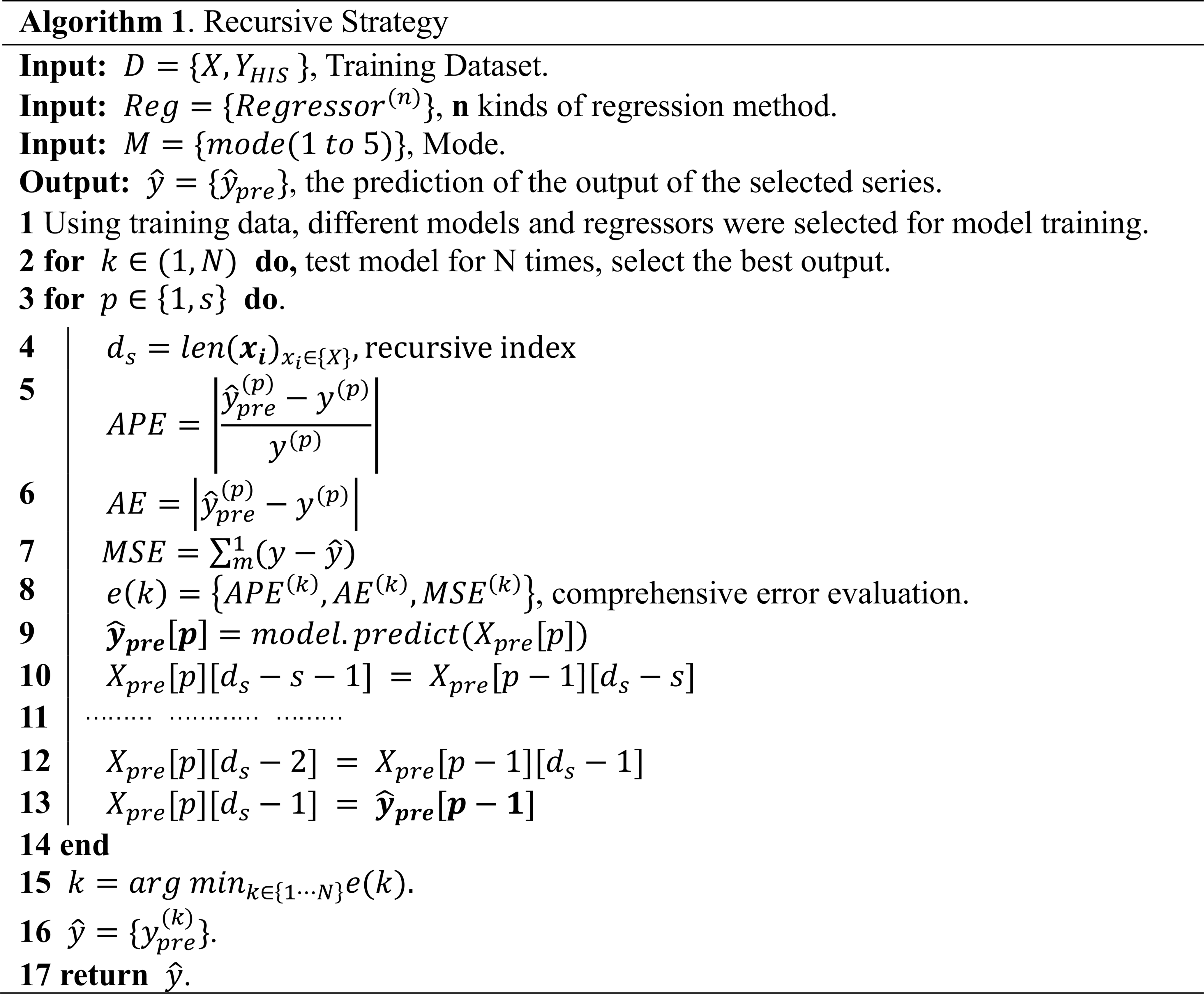
i. Recursive strategy (Rec)

The intuitive forecasting strategy is the recursive (also called iterated or multi-stage) strategy. The result of the prediction of the first step is embedded into the final element of the input vector for the subsequent prediction, and the result of the prediction of the second step is obtained. In Eq. (12), when s=1, $y_t,y_{t-\mathrm{1}},\mathrm{\dots },y_{t-n}$ can be used to predict ${\widehat{y}}_{t+\mathrm{1}}$. When s=2, the previous predicted value ${\widehat{y}}_{t+\mathrm{1}}$ is used to replace the first element of the input vector, and the following elements are replaced in turn. The original last element y_t−n is removed from the input vector. The model is iterated recursively, and the mixed vector of historical data and forecast data is used as the model input. The algorithm for this method can be expressed as in Algorithm 1. The prediction vector ${\widehat{\mathit{y}}}_{\text{pre}}\left[\mathit{p}\right]$ in the first step can be obtained based on historical data. Then the final element of the input vector X_pre[p][d_s−1] is replaced by ${\widehat{\mathit{y}}}_{\text{pre}}[\mathit{p}-\mathrm{1}]$, and the new ${\widehat{\mathit{y}}}_{\text{pre}}$ is obtained through the input model and so on, moving the value of X forward one bit and adding the new predicted value.

$$\begin{array}{}\text{(12)}& {\widehat{y}}_{t+s}=\left\{\begin{array}{ll}\widehat{f}(y_t,y_{t-\mathrm{1}},\mathrm{\dots },y_{t-n}),& s=\mathrm{1}\\ \widehat{f}({\widehat{y}}_{t+s-\mathrm{1}},y_{t+s-\mathrm{2}},\mathrm{\dots },y_{t+s-n}),& s=\mathrm{2}\\ \mathrm{⋮}\\ \widehat{f}({\widehat{y}}_{t+s-\mathrm{1}},\mathrm{\dots },{\widehat{y}}_{t+s-n}),& s\in (\mathrm{2},n]\end{array}\right.\end{array}$$

ii. Single-output coupling strategy (SOC)

The single-output coupling strategy is similar to the direct strategy proposed by Hamzacebi et al. (2009). Different machine learning models have been used to implement the direct strategy for multi-step-ahead forecasting tasks, for instance neural networks (Khashei and Bijari, 2010), nearest neighbors (Sorjamaa et al., 2007), and decision trees (Guimarães Santos and Silva, 2014). The strategy consists of forecasting each horizon independently from the others. The biggest difference from the recursive strategy is that single-output coupling does not use any approximated values to compute the forecasts, thus having no accumulation of errors. In this strategy, error in the previous prediction results will not have a great influence on the later prediction results. Each f value is supported by a corresponding model and trained with its own independent data (Eq. 13). When s=1, it is the same as one-step prediction. When s>1, the model makes prediction across the time interval of s steps. Finally, the results of single-output $y_{t+\mathrm{1}},y_{t+\mathrm{2}},\mathrm{\dots },y_{t+s-\mathrm{1}},y_{t+s}$ are coupled by Eq. (14) into a new forecast time series $[y_{t+\mathrm{1}},y_{t+\mathrm{2}},\mathrm{\dots },y_{t+s-\mathrm{1}},y_{t+s}]$.

$$\begin{array}{}\text{(13)}& {\displaystyle }{y}_{t+s}=f_s(y_t,y_{t-\mathrm{1}},\mathrm{\dots },y_{t-n+\mathrm{1}})\text{(14)}& {\displaystyle }\left\{\begin{array}{l}{y}_{t+\mathrm{1}}=f_{\mathrm{1}}(y_t,y_{t-\mathrm{1}},\mathrm{\dots },y_{t-n+\mathrm{1}})+{\mathit{b}}_i\\ y_{t+\mathrm{2}}=f_{\mathrm{2}}(y_t,y_{t-\mathrm{1}},\mathrm{\dots },y_{t-n+\mathrm{1}})+{\mathit{b}}_i\\ \mathrm{⋮}\\ \mathrm{⋮}\\ y_{t+s}=f_s(y_t,y_{t-\mathrm{1}},\mathrm{\dots },y_{t-n+\mathrm{1}})+{\mathit{b}}_i\end{array}\right.\end{array}$$

iii. Multi-output strategy (MO)

The two previous strategies (recursive and single-output coupling) may be considered single-output strategies, which neglects the existence of stochastic dependencies between future values and consequently affects the forecast accuracy. The multi-output strategy requires the design of multiple-response modeling techniques. The output is no longer a scalar quantity but a vector of length s. Using only one model, a time series of s time intervals is output (Eq. 15). Compared with single-output coupling strategy, this strategy involves simple operation and fast calculation. The disadvantage is that some regression algorithms such as Bayesian regression, gradient boosting regression trees (GBRTs), and AdaBoost do not support multidimensional output directly.

$$\begin{array}{}\text{(15)}& \begin{array}{rl}[y_{t+s},y_{t+s-\mathrm{1}},\mathrm{\dots },y_{t+\mathrm{2}},y_{t+\mathrm{1}}]=& f_{\mathrm{m}}(y_t,y_{t-\mathrm{1}},\mathrm{\dots },\\ & y_{t-n+\mathrm{2}},y_{t-n+\mathrm{1}})+{\mathit{b}}_i,\end{array}\end{array}$$

where f_m is a vector-valued function and b_i is a noise vector.

Step 6: actual-value testing

In order to prevent an over-fitting phenomenon or insufficient prediction, it is necessary to test the performance of the framework in actual waterlogging data sets after completing training and testing. N groups of continuous time series are selected for actual-value testing, and the application results with actual data will be discussed.

4 Case study

4.1 Research area

As an important city in south China and a representative of China's special economic zones, Shenzhen is one of the core cities of the Guangdong–Hong Kong–Macao Greater Bay Area.

In the process of rapid urban development, Shenzhen is also facing many challenges from natural disasters and accidents, which often bring serious threats to urban public safety and security. Shenzhen, located in the southeast coast of China, has a subtropical monsoon climate. Influenced by the Pacific monsoon current, it receives sufficient rainfall all year round. The rainfall is unusually concentrated from June to September every year, and heavy rains or extremely heavy rains occur frequently. In particular, the frontal rainfall in the Shenzhen area is subject to topography, which often forms local sudden rainstorms with short duration. According to the statistics of rainfall data in Shenzhen from 1960 to 2012, there were on average 8.8 occurrences per year of heavy rainfall with daily rainfall of more than 50 mm, 75.2 % of which were heavy rain, 21.4 % of which were torrential rain, and 3.4 % of which were extremely torrential rain (Shao et al., 2021). In May 2014, Pingshan District, Shenzhen, was hit by a sudden rainstorm, with 261 mm of rainfall in 3 h, causing 150 houses to be flooded and affecting 2600 people. The rainstorm event on 11 April 2019 saw the heaviest rainfall in April since Shenzhen began meteorological records, and it led to 11 deaths (Liu et al., 2020).

This paper focuses on the areas vulnerable to waterlogging in Shenzhen. A data-driven prediction model of urban rainstorm waterlogging depth is established, which can realize the advance perception and accurate prediction of water level change of a waterlogging point.

4.2 Step 1: data preprocessing

There are two main sources of the data used in the study. The first is the meteorological observation data of Shenzhen provided by the Shenzhen Meteorological Bureau. The data cover the time ranging from 8 March 2019 to 17 August 2020, including the meteorological observation data of rainfall, wind speed, visibility, temperature, and humidity at 242 stations in the city. The second is the waterlogging-depth sensor data of 170 observation stations in the city provided by the Water Resources Bureau of Shenzhen Municipality, with an accuracy of 1 cm. Changes in waterlogging depth affect parameters such as the refractive index and pressure. The sensor senses the changes and converts physical signals into electrical signals, which are transmitted to the database through optical fibers. The longest time range is from 1 January 2019 to 18 July 2020.

Figure 2 Waterlogging sensors and weather stations in Shenzhen.

Figure 3 Rainfall region division obtained by the Tyson polygon algorithm in Shenzhen.

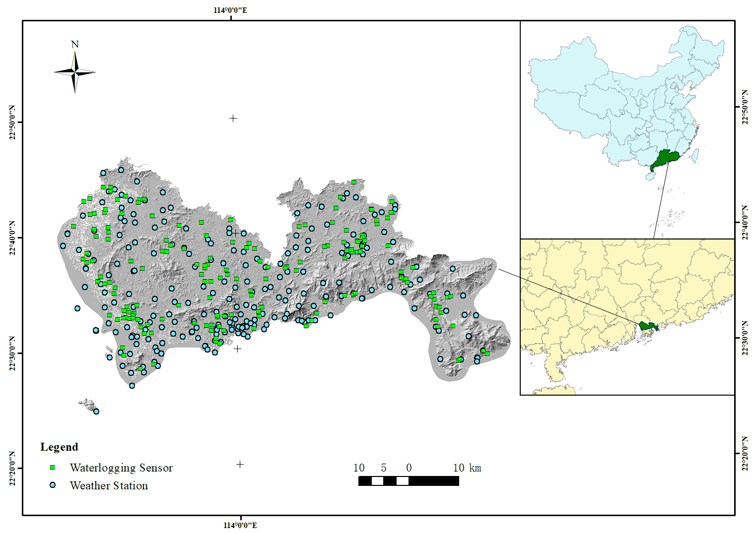
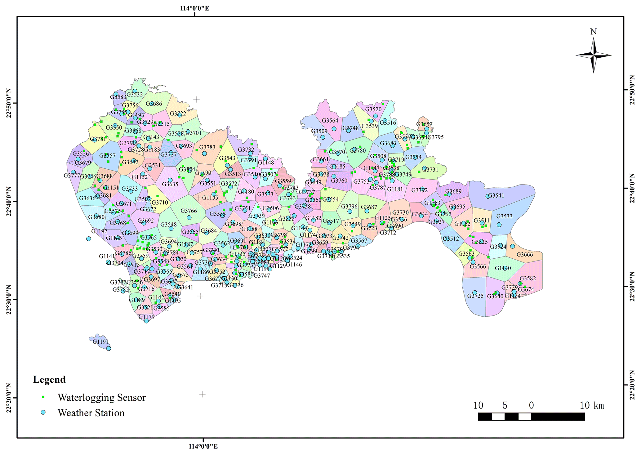
Observation points of meteorological data and waterlogging-depth data cover all 10 districts of Shenzhen, and their spatial distribution is shown in Fig. 2. The Tyson polygon algorithm is used to divide regions according to the geographical location of meteorological stations, and the rainfall coverage of each station is obtained. The polygon surface of each region indicates that meteorological data of this station are used in this region (Fig. 3) (Men et al., 2020). Through this classification form, it is determined that 170 observation stations of waterlogging depth have unique corresponding meteorological input, which unified the model input–output relationship in the spatial dimension.

Due to the fact that waterlogging sensors are configured in batches, the total operating time and data storage capacity of each sensor vary. Among 170 waterlogging sensors, we selected sensor 123, with a long operation time and a large number of data, as the research object. Through data analysis and testing the consistency of meteorological data, it has been determined that precipitation is the most influential element on waterlogging depth. Rainfall data include sliding-window rainfall with different window lengths: R10M, R30M, R01H, R02H, R03H, R06H, R12H, R24H, and R72H for 10 and 30 min and 1, 2, 3, 6, 12, 24, and 72 h of sliding-window rainfall values. D means the waterlogging depth. Through the data correlation analysis between sliding-window rainfall and waterlogging-depth data of each station (Fig. 4), it is concluded that R02H has the largest correlation degree of 0.61 with waterlogging depth. In Fig. 4, the darker the color, the lower the correlation, and the lighter the color, the higher the correlation.

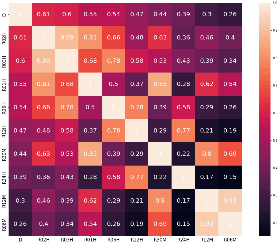
Figure 4 Data correlation analysis of rainfall data at weather station G3795 and waterlogging-depth data at sensor 123; the maximum correlation coefficient with D is 0.61 (D and R02H), and the minimum is 0.26 (D and R06M).

Due to the special working mechanism of the waterlogging-depth sensor, the data sampling rate is not uniform. In the period when there is no water accumulation (the waterlogging depth is 0), it is collected at irregular intervals of several hours or even several days. In the period when the water level changes dramatically, the sensor can collect data per minute at the fastest rate, which introduces some difficulties into our research. Considering that the interval of rainfall data is 5 min, in order to balance the model accuracy and training efficiency, the data of waterlogging depth are resampled first, which is consistent with the rainfall data on the timescale. Then data interpolation is performed on the newly added blank interval of resampling, which does not destroy the original characteristic attributes of the data. Since the fluctuation process of waterlogging is a smooth and continuous process, the waterlogging-depth curve is smooth. Five commonly used interpolation methods, cubic, quadratic, linear, zero, and nearest, are used and compared in this paper. The optimal interpolation method is determined by comparing the mean APE (MAPE) of the interpolation data Y_insert and the actual data Y_true and observing the fitting of the interpolation curve and the actual one. Finally, the linear interpolation method is applied. (Cubic and quadratic may have negative values, while zero and nearest have obvious ladder characteristics, which are not consistent with the continuous characteristics of the waterlogging depth.) After analysis, we obtain a total of 527 non-zero interpolation data points, accounting for 0.46 % of the total data set (143 424). Interpolation data are mainly concentrated at the beginning and end of the water, and the values are generally low. This part of data preprocessing unified the model input–output relationship in the time dimension, and the time range of the final rainfall and waterlogging-depth data was unified from 00:00:00 on 8 March 2019 to 23:55:00 UTC+8 on 18 July 2020 with an interval of 5 min.

After determining the location correlation between rainfall stations and waterlogging observation stations and unifying the timescale, the two data sets were integrated into one data set. From Fig. 5, it can be seen that in most of the time interval, when the rainfall is 0, the frequency of waterlogging accumulation data is lower. This is because there is no rainfall in most time intervals, which is consistent with the reality. Despite the fact that the proportion of the impervious water surface in urban construction areas increases annually, the frequency of waterlogging accumulation caused by surface runoff has decreased due to the continuous improvement of drainage system construction and the application of sponge city engineering. However, in the event of strong typhoons or heavy rain, the drainage volume still cannot meet the needs of urban drainage. This would overload the drainage system and allow large amounts of urban surface runoff to accumulate in low-lying areas. In this study, considering the factors of surface infiltration, the vegetation leaf canopy interception effect, and evaporation, surface runoff cannot be formed under extremely low rainfall and non-rainfall, so the waterlogging depth is always 0. In order to avoid the interference of such factors with model training, the minimum rainfall threshold is set here as 5 mm. By searching the entire data set and locking the start and end time stamps of each rainfall event interval, named R_STA and R_END, rainfall duration is denoted by R_DUR. In the entire data set, R_STA and R_END are paired to represent the rainfall start and end index. A total of 251 rainfall event time series (982.34 h in total; average rainfall duration is 3.91 h) were obtained by screening 143 424 data points from this site, and a new data set Rain_Set with 12 309 data points (Fig. 6) was constructed. This method eliminates the interference of a large number of sunny weather inputs to the model, which is proved to improve the efficiency and accuracy of the model calculation.

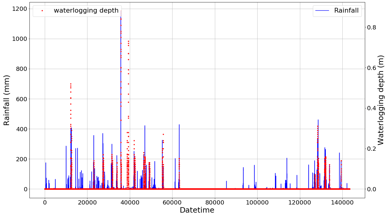
Figure 5 Rainfall and waterlogging from 00:00:00 on 8 March 2019 to 23:55:00 on 18 July 2020 (with an interval of 5 min). Each x-axis data point represents 5 min.

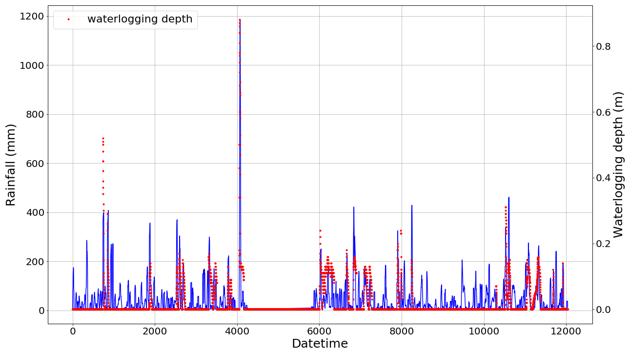
Figure 6 Rainfall (solid blue line) and waterlogging (dotted red line) according to Rain_Set.

Table 1 Modes (1) to (5) with different m and n parameters.

4.3 Step 2: training-mode setting

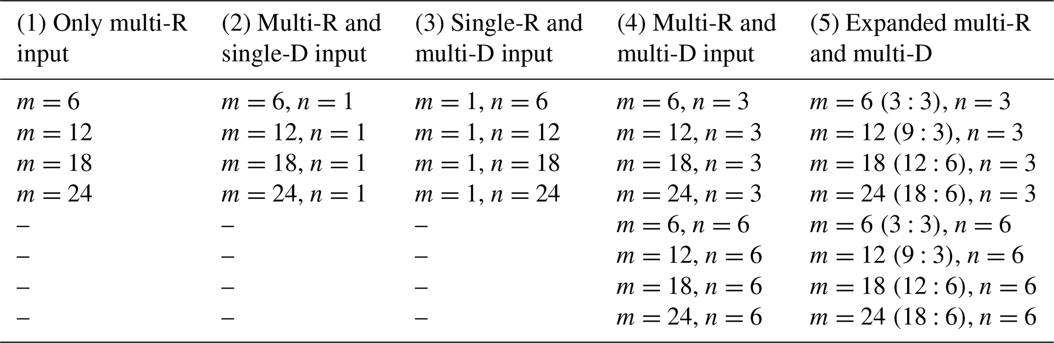
Based on the MSMWP framework, after data preprocessing, different training modes are constructed by changing ϕ to adjust the R-and-D combination mode. Each rainfall time series is processed by cyclically cutting in the form of sliding windows; we can obtain a matrix R as Eq. (16). In the five modes, input vectors of different dimensions can be constructed by adjusting the values of m and n, and multiple models can be trained. The goal of the model is to accurately predict the waterlogging depth at a certain time. Assume that the current time is t and the predicted target value of the waterlogging depth in the future is $y_{t+\mathrm{1}},y_{t+\mathrm{2}},y_{t+\mathrm{3}},\mathrm{\dots },y_{t+s-\mathrm{1}},y_{t+s}$. When m=6 and n=1, the model selects rainfall in 30 min and waterlogging in 5 min before time t as input for training. When m=12 and n=3, the model selects the rainfall in 1 h and waterlogging in 15 min before time t as input for training. Under different combination conditions of m and n, the five combination modes are selected as shown in Table 1:

$$\begin{array}{}\text{(16)}& \begin{array}{rl}& \text{rainfall set}\\ & \mathbf{R}=\left[\begin{array}{ccccccccc}\mathrm{5}& \mathrm{18}& \mathrm{41}& \mathrm{63}& \mathrm{\dots }& \mathrm{97}& \mathrm{99}& \mathrm{130}& \mathrm{147}\\ \mathrm{18}& \mathrm{41}& \mathrm{63}& \mathrm{74}& \mathrm{\dots }& \mathrm{99}& \mathrm{130}& \mathrm{147}& \mathrm{151}\\ \mathrm{41}& \mathrm{63}& \mathrm{74}& \mathrm{83}& \mathrm{\dots }& \mathrm{130}& \mathrm{147}& \mathrm{151}& \mathrm{158}\\ \mathrm{\dots }& \mathrm{\dots }& \mathrm{\dots }& \mathrm{\dots }& \mathrm{\dots }& \mathrm{\dots }& \mathrm{\dots }& \mathrm{\dots }& \mathrm{\dots }\\ \mathrm{6}& \mathrm{4}& \mathrm{2}& \mathrm{1}& \mathrm{\dots }& \mathrm{\dots }& \mathrm{0}& \mathrm{0}& \mathrm{0}\\ \mathrm{4}& \mathrm{2}& \mathrm{1}& \mathrm{1}& \mathrm{\dots }& \mathrm{\dots }& \mathrm{0}& \mathrm{0}& \mathrm{0}\end{array}\right].\end{array}\end{array}$$

Since rainfall is the fundamental factor affecting waterlogging, the dimension of rainfall in the latter two modes is basically higher than that of waterlogging. In expanded multi-R and multi-D, the rainfall input is split with t as the dividing line to emphasize the influence of the subsequent continuous rainfall input on the model. For example, $m=\mathrm{12}(\mathrm{9}:\mathrm{3})$ means that rainfall 45 min before t and rainfall 15 min after t are selected as input.

The strategy in Step 5 influences the label selection of the model. The recursive strategy requires direct prediction of y_t+1 and then recursion with label y_t+1.

4.4 Step 3: machine learning regressor setting

In this paper, eight regression algorithms are selected. They are linear regression (LR), tree regression (TR), random forest regression (RFR), k-nearest neighbors regression (KNN), ridge regression (RR), kernel ridge regression (KRR), lasso regression (LaR), and elastic net (ETN) and can simultaneously perform one-dimensional and multidimensional regression output.

4.5 Step 4: evaluation of model performance

The data set constructed was divided into a training set and test set at a ratio of 70 % and 30 %. Different modes, strategies, and regression algorithms were applied for training and evaluated by RMSE, MAE, and the R² score. The curve fitting of the predicted data on the test set was compared with the actual data, and the test results of each configuration were analyzed and sorted.

$$\begin{array}{}\text{(17)}& {\displaystyle }\text{MAE}={\displaystyle \frac{\mathrm{1}}{m}}\sum _{i=\mathrm{1}}^m\left|{\widehat{y}}^{\left(i\right)}-y^{\left(i\right)}\right|\text{(18)}& {\displaystyle }\text{RMSE}=\sqrt{{\displaystyle \frac{\mathrm{1}}{m}}\sum _{i=\mathrm{1}}^m({\widehat{y}}^{\left(i\right)}-y^{\left(i\right)}{)}^{\mathrm{2}}}\text{(19)}& {\displaystyle }{R}^{\mathrm{2}}=\mathrm{1}-{\displaystyle \frac{{\sum }_i({\widehat{y}}^{\left(i\right)}-y^{\left(i\right)}{)}^{\mathrm{2}}}{{\sum }_i(\stackrel{\mathrm{‾}}{y}-y^{\left(i\right)}{)}^{\mathrm{2}}}}\end{array}$$

4.6 Step 5: prediction strategy setting

The Rec policy is set to replace only the last value of the waterlogging vector at a time. The single-output coupling strategy outputs at 5 and 10 min until the moment (s×5) min of waterlogging, so the label is $y_{t+\mathrm{1}},y_{t+\mathrm{2}},y_{t+\mathrm{3}},\mathrm{\dots },y_{t+s}$. The multi-output strategy outputs the waterlogging value vector of minutes at (5 to s × 5) at the same time, so its label is $[y_{t+\mathrm{1}},y_{t+\mathrm{2}},y_{t+\mathrm{3}},\mathrm{\dots },y_{t+s}]$.

4.7 Results and discussion

This section presents and discusses the testing results of the different mode and forecasting strategies. For each mode, we report the results obtained with the eight different regression methods. Based on the results of actual-value verification, different prediction strategies are discussed.

4.7.1 Testing results

The time series intercepted with rainfall events were integrated into a new data set, with a total of 12 039 data points. The first 70 % constituted a training set with 8428 points of data, and the last 30 % constituted a testing set with 3611 points of data. In the testing set, eight regression methods were used to test five modes, and the model structure inside each mode was changed by adjusting the input parameters m and n. The testing results of different modes are shown in Tables A1 to A4. The numbers in parentheses represent the ranking of evaluation indicators (MAE, RMSE, R² score) among different modes of the same algorithm. Bold font indicates the top results of the same algorithm with different modes. The italic number indicates that the indicator is in the top 50 % of the best results (bold) between different algorithms. Taking mode (3) – KRR – as an example, in the KRR optimal indicator, RMSE is 0.0051 ranking second; MAE is 0.0013, ranking third; and the R² score is 0.9779, ranking third, so the italic indicator of KRR is 3.

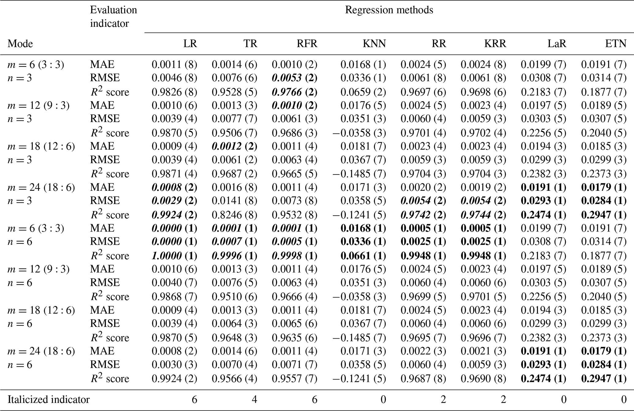
Table 2 Testing results of mode (5), expanded multi-R and multi-D. The numbers in parentheses represent the ranking of evaluation indicators (MAE, RMSE, R² score) among different modes of the same algorithm. Bold font indicates the top results of the same algorithm with different modes. Italic numbers indicate that the indicator is in the top 50 % of the best results (bold) between different algorithms.

Figure 7 Testing results using the LR and KRR methods when m=18.

Among the five modes, mode (1) only uses rainfall data to predict waterlogging accumulation and has the worst testing result. When m changes from 6 to 24, the R² score of RR changes from 0.1209 to 0.3954, which is 3.27 times the initial value. In this mode, the larger m is, the more information the model learns and the better the testing performance is. By comparing the predicted value with the actual value, the results of the eight kinds of regression methods all have large noise when the actual waterlogging depth is 0. Even though KRR and LR can achieve good trend prediction at the peak, there are still large noise fluctuations most of the time (Fig. 7). This phenomenon may be caused by the lack of historical waterlogging time series input, so the noise suppression is not good.

In mode (2), the prediction performance of LR and TR becomes better as m increases, which is the same as mode (1). However, RFR, RR, and KRR are not sensitive to parameter changes.

In mode (3), the larger the parameter n is, the better the model may not be. For example, the optimal results of RFR, RR and KRR are obtained when n=6, while the R² score of the three exceeds 0.977, indicating that the early information of waterlogging depth is not helpful to the prediction of waterlogging depth in the future and may cause some interference. For LR, with the same number of parameters, the result of mode (3) is better than that of mode (2). The main reason for this is that mode (3) extracted more historical waterlogging-depth information, which changes by a continuous process in short-term prediction. However, this does not mean that the model has the best performance, because it contains insufficient rainfall information and may not perform well in the practical application of prediction.

Mode (4) coupled multiple rainfall and waterlogging inputs. Overall, the results of mode (4) are better than those of modes (2) and (3) with one-dimensional input (m=1 or n=1). In this mode, the TR and RFR methods achieved the best testing results. TR achieved a 0.9778 R² score and 0.0050 RMSE (m=24, n=3). The R² score and RMSE of RFR reached 0.9803 and 0.0049 respectively (m=6, n=3).

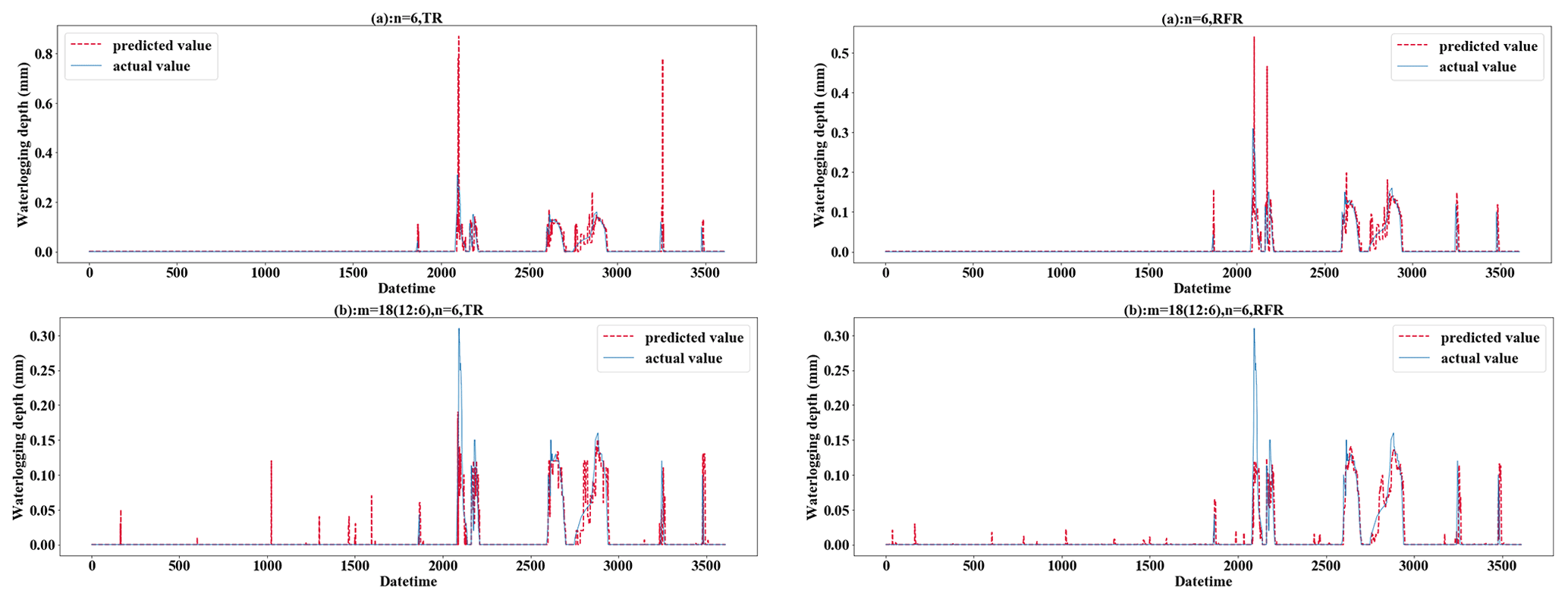
Figure 8 Testing results of mode (5) and only-D prediction using TR and RFR (when n=6 for both).

Figure 9 Testing results using different methods when m=24 and n=3. (a) For KRR; (b) for LR; (c) for RFR; (d) for TR.

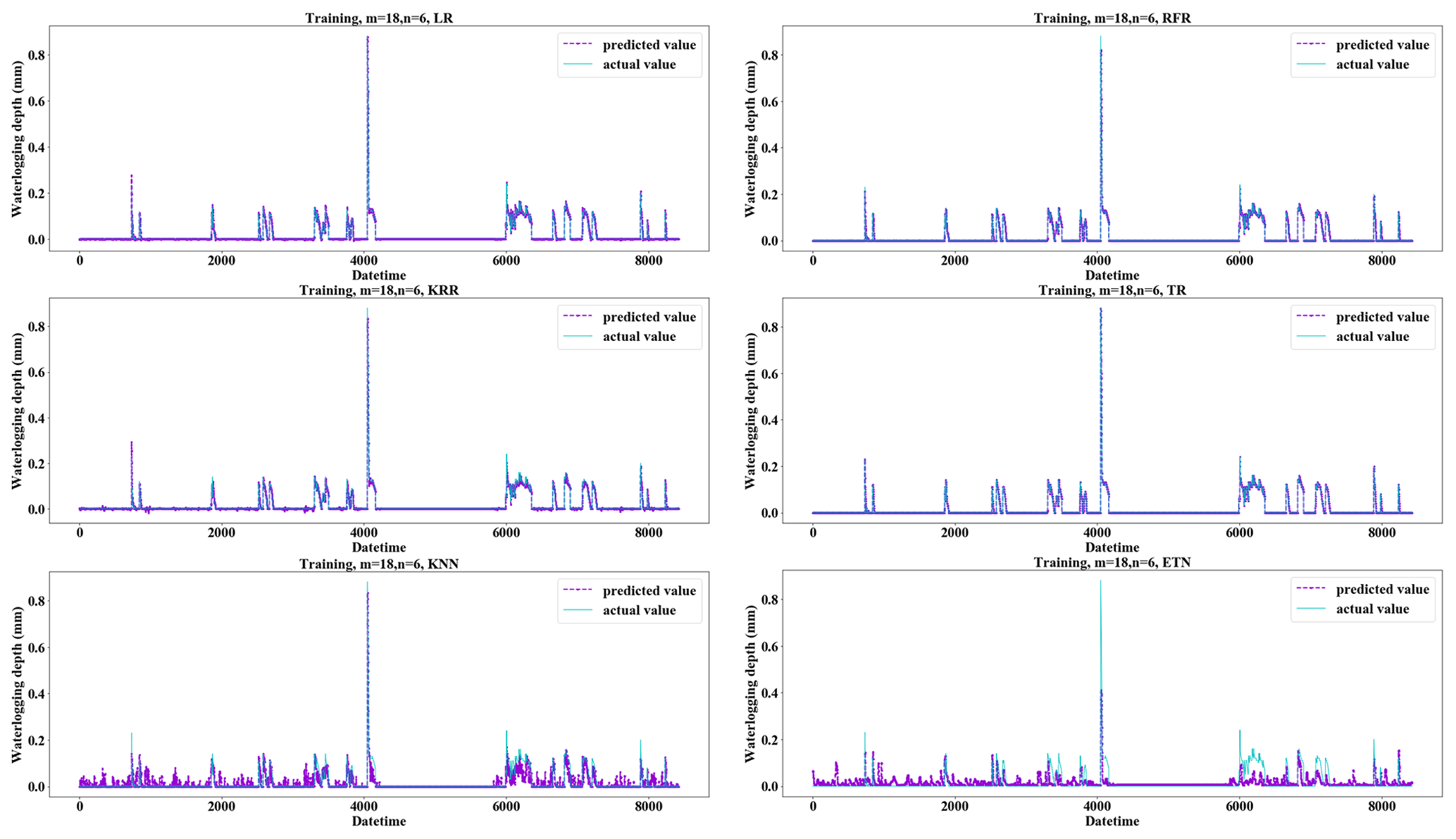
Figure 10 Fitting performance of different regression methods applied to the training set when m=18 and n=6.

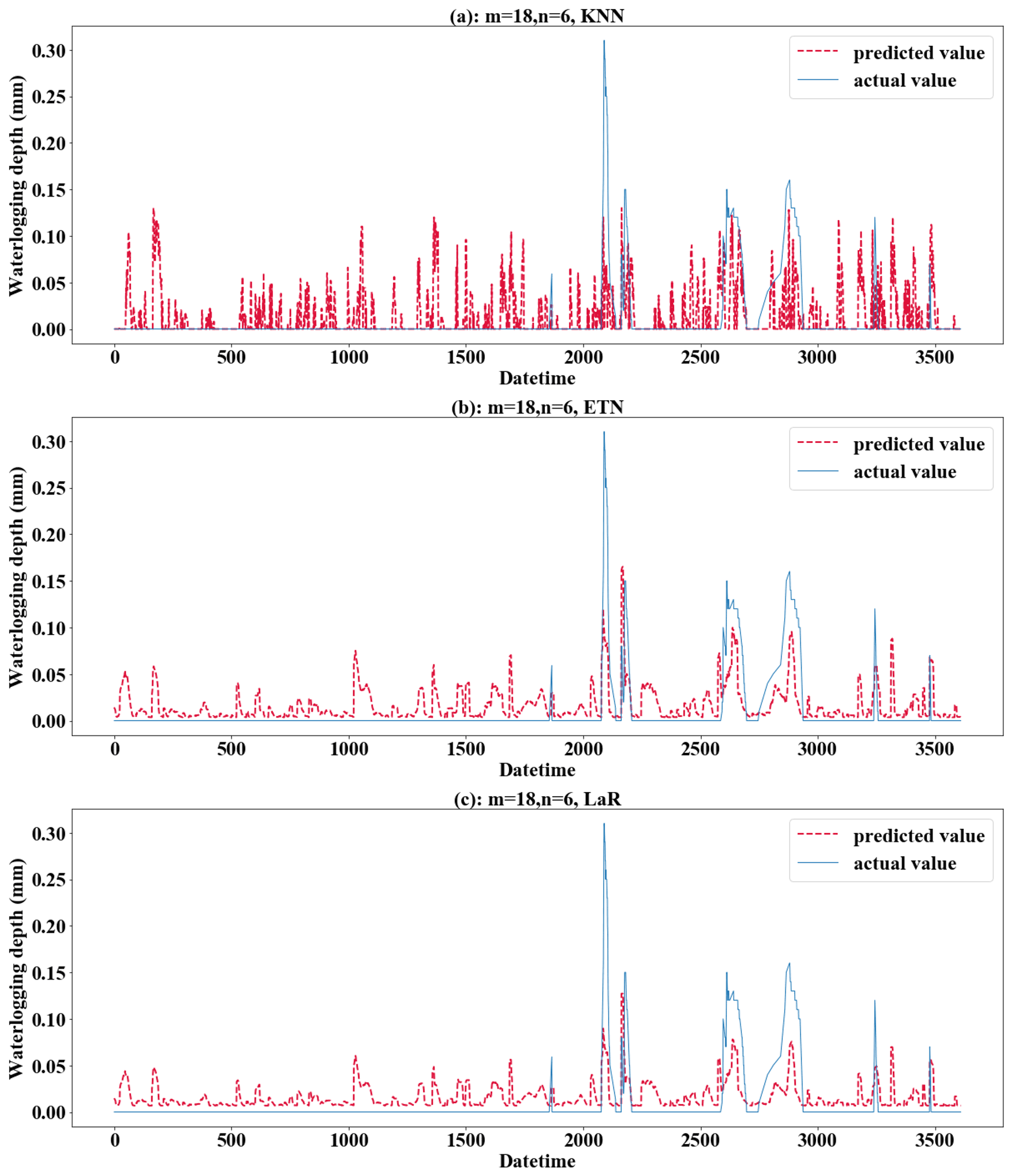
Figure 11 Performance of the KNN, ETN, and LaR methods applied to the testing set when m=18 and n=6. (a) For KNN; (b) for ETN; (c) for LaR.

Figure 12 Actual-value verification time series from 26 May 2020, 13:00 to 17:30.

Mode (5) expanded the rainfall input and considered the influence of future rainfall. When parameters are adjusted to m=6 (3:3) and n=6, the LR evaluation indicator (MAE=0, RMSE=0, and R² score=1) is abnormal. This problem also exists in RFR, TR, etc. The main reason for this is that the prediction label has been included in the input time series, so the result of m=6 (3:3) and n=6 in mode (5) should be removed in the discussion. Based on the performance of mode (5) for the test set, the performance of mode (5) will improve after the predicted time is expanded. The reason for this is that mode (5) expands the rainfall input and considers the influence of future rainfall. Especially the rainfall model with short duration and high intensity is more suitable for this mode. As shown in Fig. 8, (a) only 30 min of waterlogging data was used for prediction and (b) 30 min of waterlogging with 90 min of expanded rainfall was used as input. With the increase in prediction time, the difference in prediction performance between them increases gradually. In the prediction of 40 min waterlogging, the R² score of (b) (0.6841) is 2.4 times that of (a) (0.2847) when the TR method is applied. Using the RFR method, the R² score and MAE of (b) (R² score = 0.7428, MAE = 0.0044) also significantly exceeds (a) (R² score = 0.6488, MAE = 0.0053). Especially for the prediction of medium–high values, in the case of a high value (0.30 m) and medium value (0.13 m), the prediction results of (a) are 0.82 m and 0.73 m, and the large error leads to poor accuracy in the prediction of medium- to large-scale waterlogging.

From the perspective of the comparison of regression methods, the performances of LR, TR, RFR, RR, and KRR are relatively good, which is reflected in the strong generalization ability of the model (Fig. 9). KRR, as ridge regression with a kernel function added, is more suitable for high-dimensional data. In this study, it shows a slightly stronger regression performance than RR. It can be seen from the comparison (Fig. 9a and b) that LR and KRR have strong prediction ability for high values but poor noise suppression for low values and 0 values, and the model fluctuates constantly around the x axis. The prediction of RFR for the highest value is insufficient, but the prediction performance for other high values is better. Its noise control for low values is better. TR has the best noise control effect for a 0 value, but the curve is not smooth or ladder shaped at high values. Of course, this is related to the principle of the algorithm. When applying RFR, selecting the parameter n_estimators which is equal to 100 can solve the problem of TR (Fig. 9c). LR, RFR, KRR, and TR show strong fitting ability in the training set (TR has MAE = 0.0000, RMSE = 0.0000, and R² score = 1.0000) (Fig. 10); KNN and ETN show relatively poor fitting ability. KNN, LaR, and ETN have weak ability of fitting and generalization and are not suitable for regression prediction of such data (Fig. 11). KNN methods have a negative R² score in mode (1), mode (2), mode (4), and mode (5). For most data sets with eigenvalues of 0, the prediction performance is often poor, which can explain why the results of the KNN method are the worst (Fig. 11a). LaR and ETN are mode-insensitive and have the same results in modes (1) and (2). However, within each mode, as m and n change, the results will be different. The poor results of the LaR method (Fig. 11c) may be because the method is suitable for multi-variable models and the variables are selected by adjusting the λ value to change the compression variable coefficient, but there are fewer variables in this study. Similarly, considering that ETN (Fig. 11b) works well when many features are interconnected, this model has a small number of features and the model with similar basic principles to lasso regression also has poor performance.

To sum up, mode (5) performs better than any other modes, indicating that the short-term prediction of waterlogging considering the change in the future rainfall trend is more realistic. LR seems to have achieved good prediction results in all five modes. However, the factor that cannot be ignored is that the original waterlogging-depth data are sparse and uneven, which must be due to resampling interpolation processing. It is necessary to go through an actual-value test to judge whether the LR method is really applicable to prediction.

4.7.2 Step 6: actual-value verification

Actual-value verification takes a subset of the testing set, so the first 85 % of the full data set is selected as the training set, which can increase the number of training samples and improve the training ability of the model. The time series from 26 May 2020 at 13:00 to 26 May 2020 at 17:30 was selected, lasting 4.5 h (Fig. 12), covering the complete process of waterlogging fluctuation. In this way, the waterlogging-depth prediction ability of the model can be verified. The changes in rainfall and waterlogging in this period are shown in Fig. 12. The time series was divided into six groups on average. The waterlogging-depth changes of 30 min were predicted by six sequential steps.

In order to highlight the prediction performance of each strategy, we set s=6 for 30 min prediction. That is a long forecast for real-time water levels. In practical application, 15 to 20 min prediction may be a common prediction time, and 20 min prediction has fully met the requirement of releasing early warning information in advance and dispatching the nearest traffic and fire personnel to the scene for disposal (Georgiadou et al., 2010). We will make evaluation from multiple indicators such as absolute error (AE), absolute percent error (APE), and time cost. Mode (5) with m=18 (12:6) and n=6 was selected as the basic parameters of the model to evaluate the model performance under each strategy. Figure A1 in the Appendix represents the isometric segmentation of the verification data set with different strategies. The first 30 min of the time series is taken to show the curves between the actual values in each group and the predicted values for each method. KNN, LaR, and ETN perform poorly in the application of prediction and have high values of AE and APE. Therefore, we will not discuss these three poor methods in the analysis of results. The absolute error of the predicted value and actual value of each strategy was also discussed (Fig. A2). We set a tolerance of 0.02 m to exclude reasonable error. APE reflects the accuracy of the model, but at low values it does not independently reflect the performance of the model because even small errors (< 0.01 m) can cause APE to rise (Fig. A3). Therefore, the mean value of AE and APE (MAE and MAPE) was used to evaluate the model accuracy, and the variance in AE and APE (V-AE and V-APE) was used to evaluate the robustness. Since real-time sensor data are used in prediction, continuous calculation is required to update the model. Time cost is adopted as an indicator to evaluate the continuous computing capability of the model.

Table 3 Model performance using the Rec strategy. EI denotes evaluation indicator. “S” denotes segments.

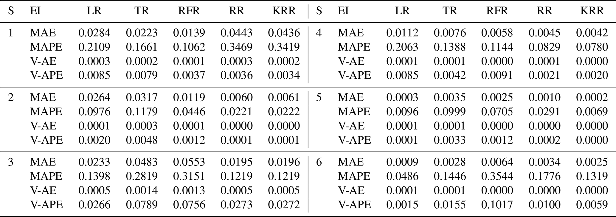
Table 4 Model performance using SOC strategy. EI denotes evaluation indicator.

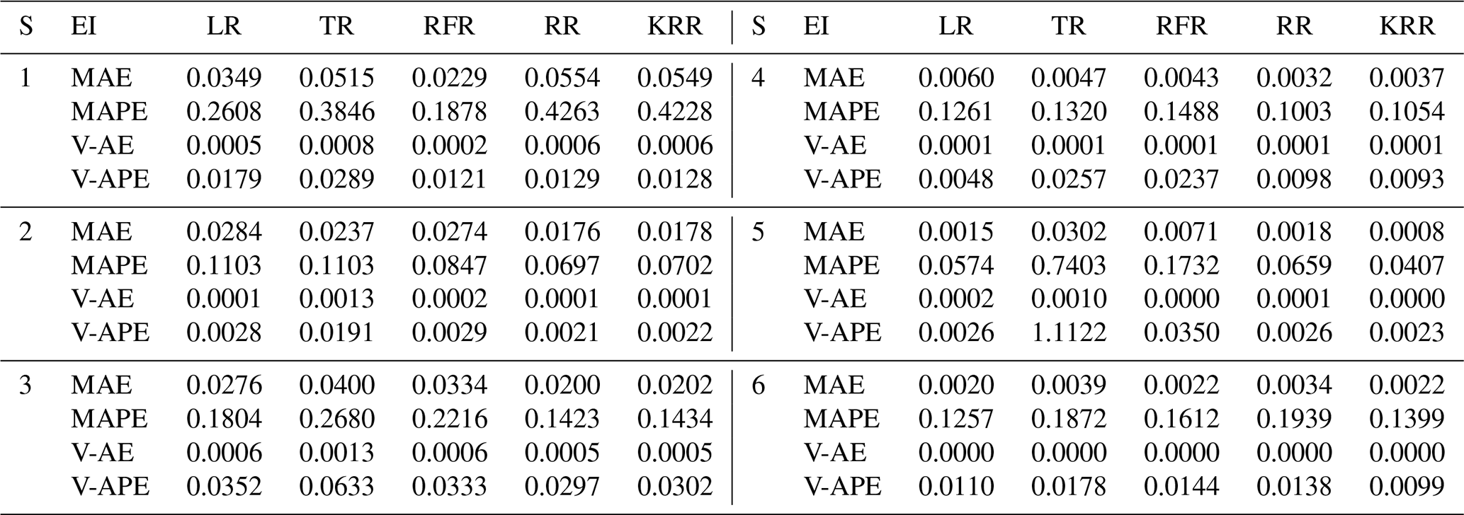
Table 5 Model performance using MO strategy. EI denotes evaluation indicator.

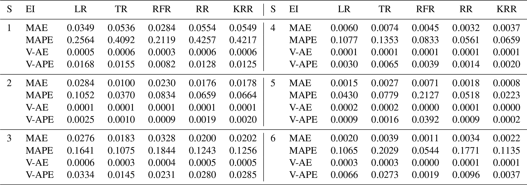
Table 6 Model performance statistics with different strategies applied. TimeC denotes time cost. Bold is the optimal indicator for different regression methods and prediction strategies.

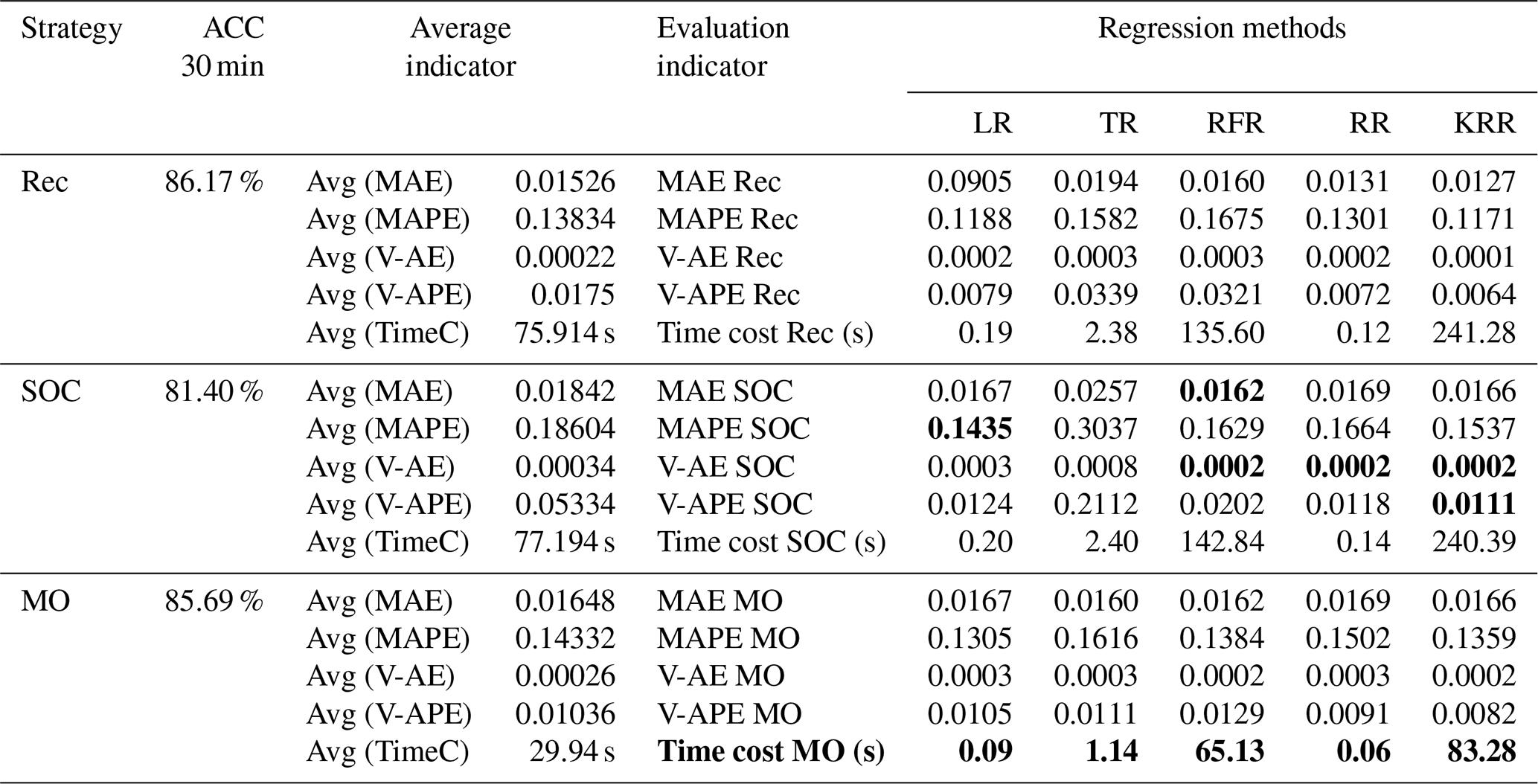
Tables 3 to 5 show the evaluation results of different strategies. As seen in Table 6, MAE of the Rec strategy is 0.0153 m, which is better than 0.0184 m of the SOC and 0.0165 m of the MO strategies. Of course, the MAE of the three is within the tolerance (0.02 m). Under the Rec strategy, the model replaces the last data point of the input vector with the predicted value every step. The reason for the optimal Rec result is that the fluctuation of the waterlogging is basically a monotonically increasing or decreasing process, and generally there is no fluctuation in a short period of time. In addition, the input vector is long enough to minimize the cumulative error caused by the predicted value deviation. The application of recursive algorithm can better continue the prediction trend of the model, so the MAE result of Rec is the best.

Rec and MO strategies have better performance and robustness. Rec and MO have lower MAPE, corresponding accuracy can reach 86.1 % and 85.7 %. The accuracy of SOC was only 81.4 %. The primary cause of this phenomena is the operating process of SOC, which combines the findings of six distinct models into a final prediction vector. When predicting the s step, there will be a loss of y_t+1, y_t+2, …, y_t+s−1 in the middle, resulting in a large error in the following part. In contrast, the V-AE and V-APE of the SOC strategy are the lowest, indicating poor performance and model robustness.

MO has the best V-APE (0.01036), indicating that the accuracy of this strategy has the smallest fluctuation, and the model has the best robustness. The V-AE (0.00026) of Rec was similar to that of MO (0.00022), but the V-APE of Rec was 69 % larger than that of MO. The reason is that APE fluctuated greatly when TR and RFR were applied under Rec strategy, and V-APE was 3.05 times and 2.49 times of MO strategy respectively. Therefore, we infer that under the same conditions, the decision tree algorithm has smaller fluctuation when applied to multidimensional output and can obtain better robustness.

Considering the time cost, the model must be updated within the 5 min interval for data prediction. This paper used tower workstation with 8 core Intel(R) Xeon(R) W-2123 3.60 GHz CPU, 64.0 GB RAM and NIVDIA Quadro RTX4000 GPU. MO strategy has a faster speed in calculation. The average time cost of Rec and SOC is about 2.54 times that of MO. Under the MO strategy, the output form of the model is a six-dimension vector. The advantage of this strategy is that it only needs to perform one training and prediction process and does not need recursion or multiple model coupling, so it is more convenient to use. Therefore, the calculation time of each regression method is greatly reduced. The time cost of KRR was shortened from 240.39 to 83.28 s. It should be noted that although the KRR algorithm has good model performance and robustness, its time cost is too high, reaching 241.28 s under the Rec strategy, which makes it difficult to meet the requirements of update calculation within 5 min. LR, TR, and RR can all be updated within 3 s due to their simple structures. RFR has a high time cost because it has to traverse all trees. However, it can meet the requirement of the update time (only 65.13 s under MO strategy).

In conclusion, LR, TR, RFR, RR, and KRR are superior to other methods, which is consistent with the results based on the testing set. Models using Rec or MO strategies have better performance and robustness, with average accuracy more than 85 % for predicting waterlogging depth in the next 30 min. For short-term prediction, such as 15 min prediction, the accuracy can reach 93 %, and the robustness of the model will be further improved. As can be seen from Figs. A1 to A3, when s=3, the prediction curves of RFR, LR, KRR, and other methods basically match actual values, and AE and APE of each group are almost within tolerance.

5 Conclusions

The prediction and early warning of urban rainstorm and waterlogging disaster have always constituted a key problem. It is challenging and meaningful to predict the rapid water level rise caused by short-term heavy rainfall in advance.

Waterlogging caused by rainstorms usually accumulates in low-lying areas of cities, such as poorly drained blocks and roads, underpass tunnels, bridge culverts, municipal plumbing manholes, and underground shopping malls or parking lots. Accurate prediction of waterlogging is essential for emergency decision-making and disaster response. Government emergency departments can issue timely warning information to the public and notify traffic management departments to rush to the scene to block the relevant roads, culverts, tunnels, etc. Effective prediction and monitoring will help minimize casualties and property losses.

A multi-strategy-mode waterlogging-prediction framework for waterlogging is proposed, which contains how to preprocess raw data and select training modes for different machine learning algorithms. In this framework, different prediction strategies are discussed and used to predict multiple dimensions of waterlogging. Results show that the mode of expanded multi-R and multi-D performs better than any other mode; five regression algorithms are more suitable for waterlogging prediction. Recursive and multi-output strategies have better performance and robustness, but the MO prediction strategy not only has higher performance but also is more efficient. We note that the recursive strategy is poor in the research of Ben Taieb et al. (2012). This is mainly because of the periodic characteristics of the data. In this study, physical characteristics of waterlogging determine that water level change is generally a monotonically increasing or decreasing process, so Rec can also have a good performance in the prediction of non-periodic data with obvious trends.

In this paper, we were concerned only with the lead time for an identified site. In the future, increasing the number of sensors could improve the geographic information of waterlogging point locations, including more DEM, slope, positive and negative terrain, infiltration rate, and other information. This kind of model can be extended to the spatial dimension for prediction. Through grid analysis, all position points in the study area can be traversed and a waterlogging risk map can be drawn.

Appendix A

Table A1 Testing results of mode (1), only multi-R input. The numbers in parentheses represent the ranking of evaluation indicators (MAE, RMSE, R² score) among different modes of the same algorithm. Bold font indicates the top results of the same algorithm with different modes. The italic number indicates that the indicator is in the top 50 % of the best results (bold) between different algorithms.

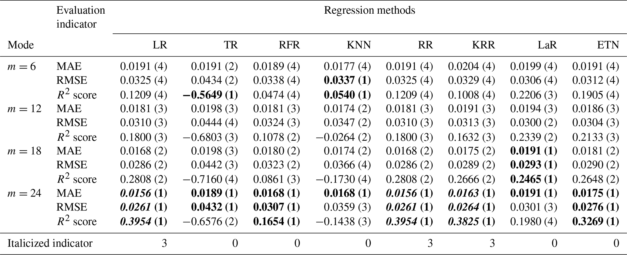
Table A2 Testing results of mode (2), multi-R and single-D input. The numbers in parentheses represent the ranking of evaluation indicators (MAE, RMSE, R² score) among different modes of the same algorithm. Bold font indicates the top results of the same algorithm with different modes. The italic number indicates that the indicator is in the top 50 % of the best results (bold) between different algorithms.

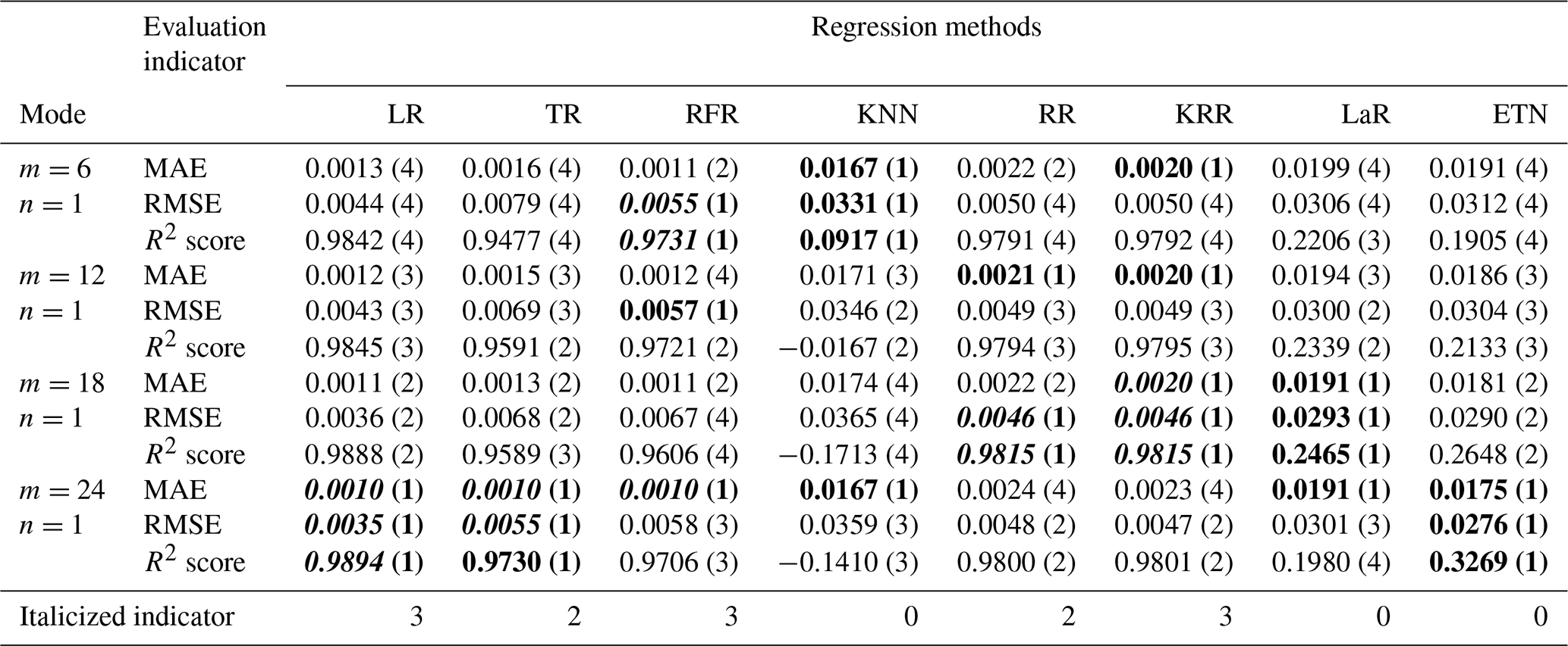
Table A3 Testing results of mode (3), single-R and multi-D input. The numbers in parentheses represent the ranking of evaluation indicators (MAE, RMSE, R² score) among different modes of the same algorithm. Bold font indicates the top results of the same algorithm with different modes. The italic number indicates that the indicator is in the top 50 % of the best results (bold) between different algorithms.

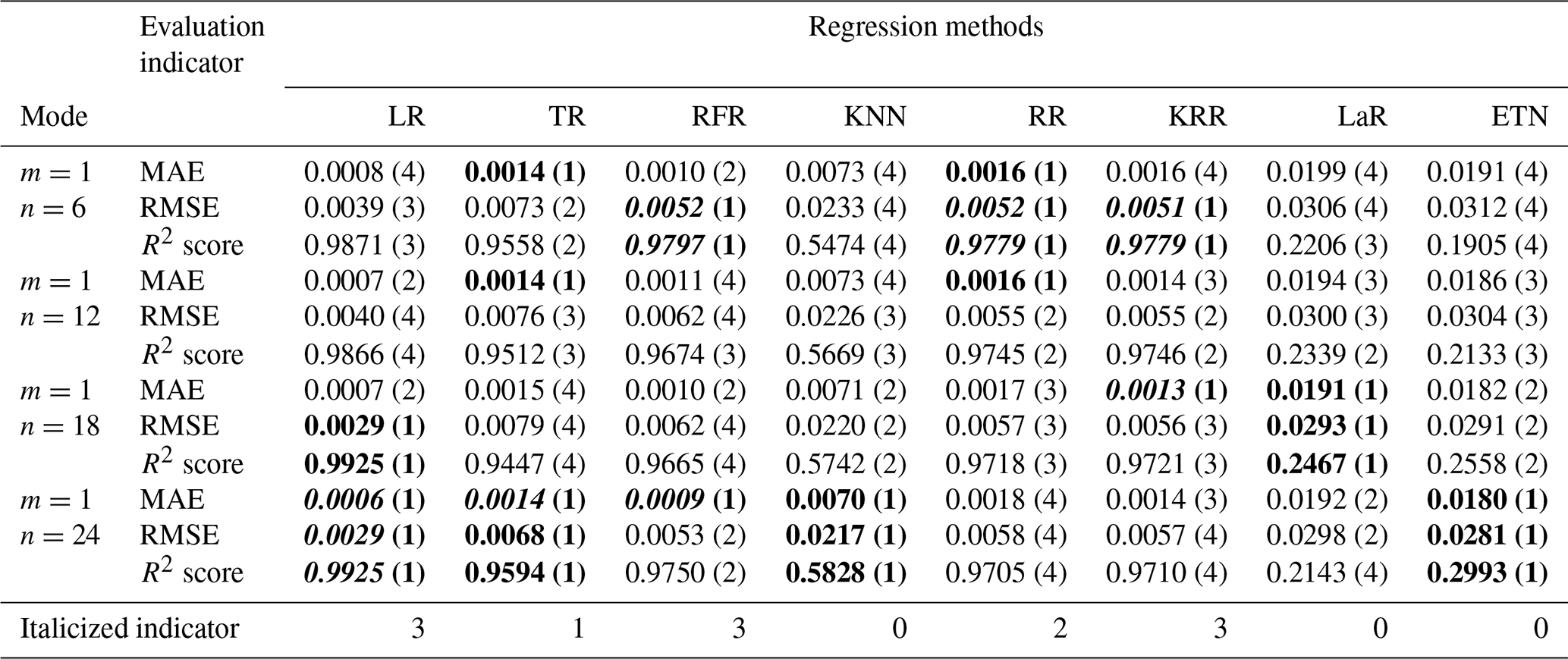
Table A4 Testing results of mode (4), multi-R and multi-D input. The numbers in parentheses represent the ranking of evaluation indicators (MAE, RMSE, R² score) among different modes of the same algorithm. Bold font indicates the top results of the same algorithm with different modes. The italic number indicates that the indicator is in the top 50 % of the best results (bold) between different algorithms.

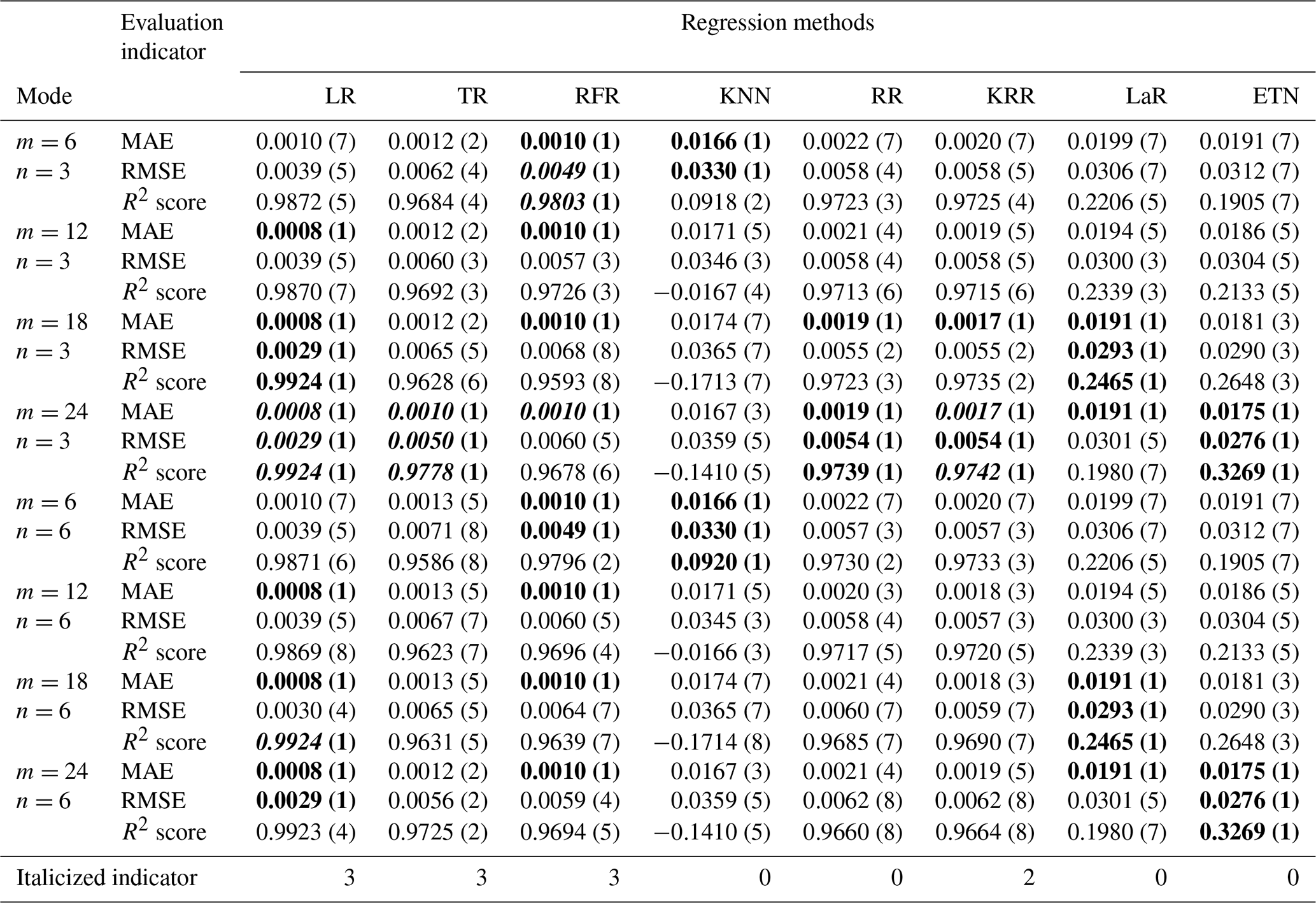
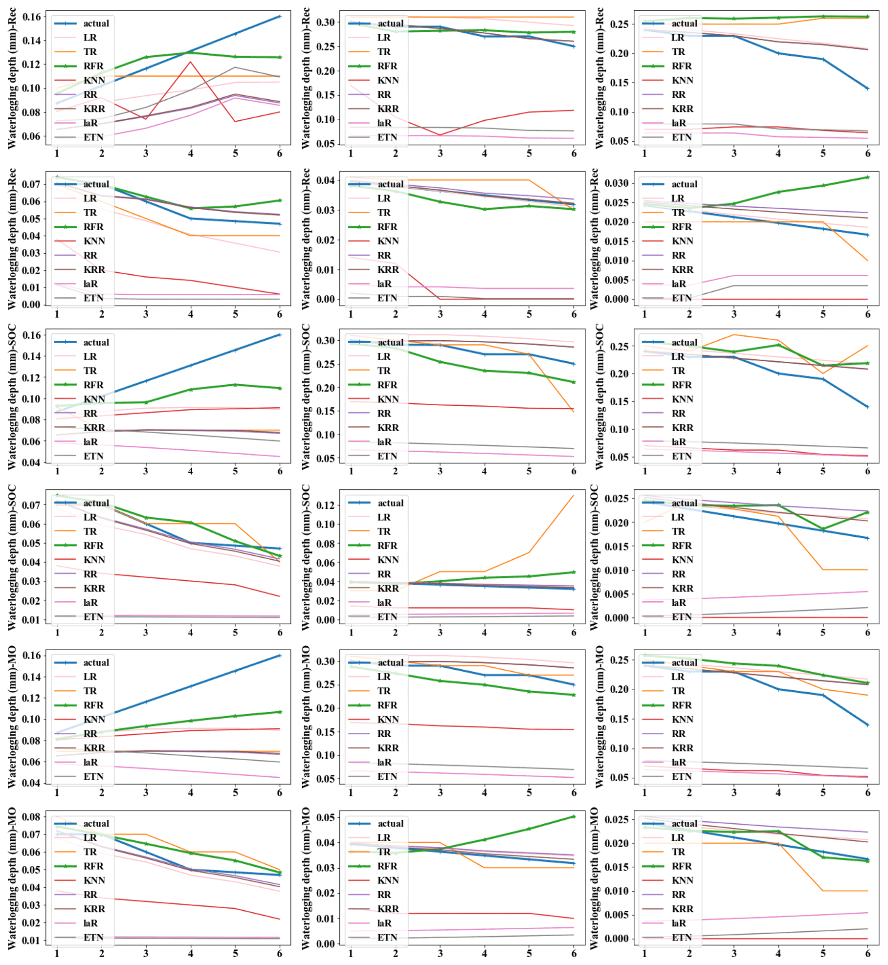
Figure A1 Predicted values and actual values of different strategies. (The x axis represents predicted steps within each group.)

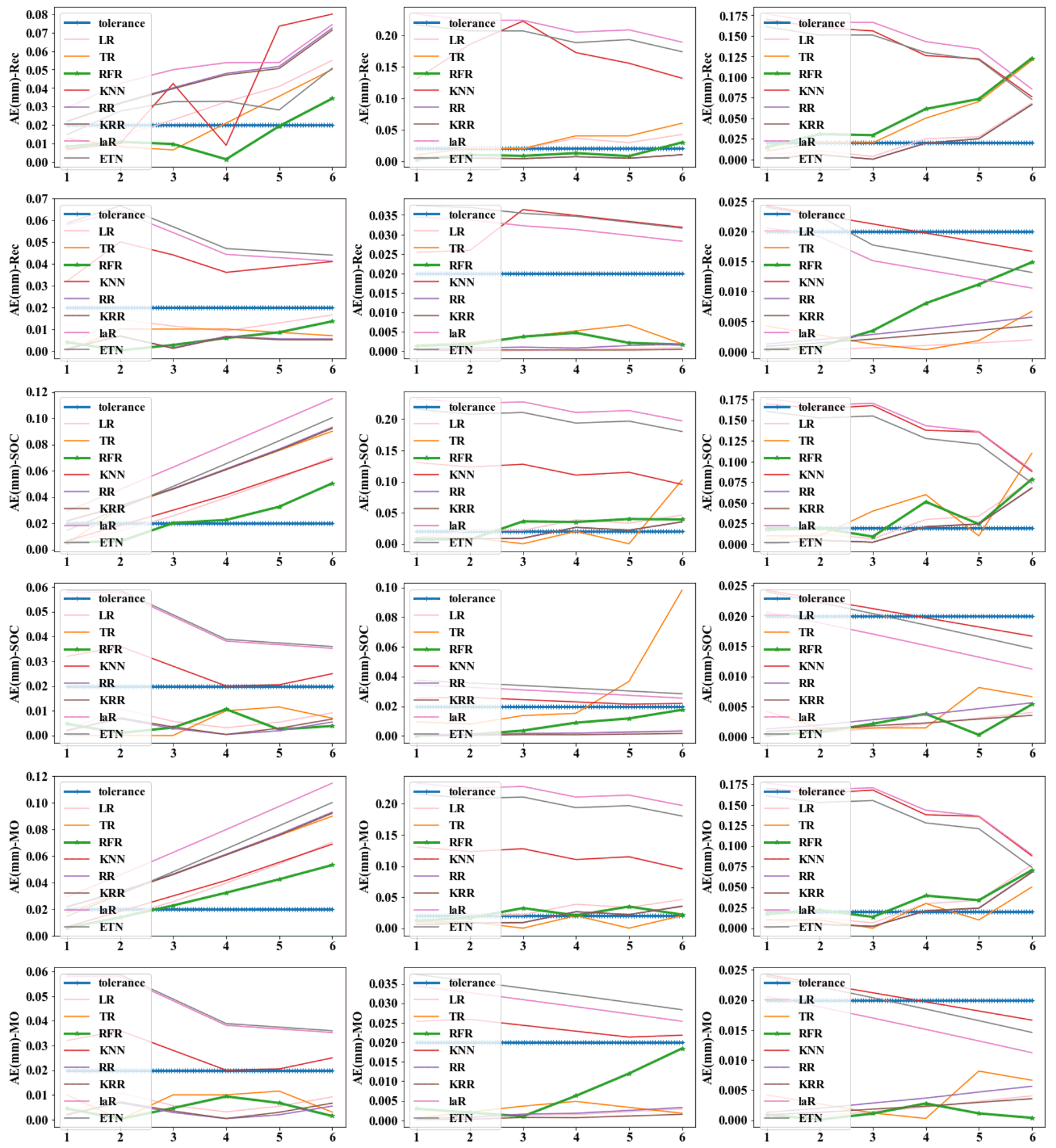
Figure A2 Absolute error (AE) of different strategies. (The x axis represents predicted steps within each group.)

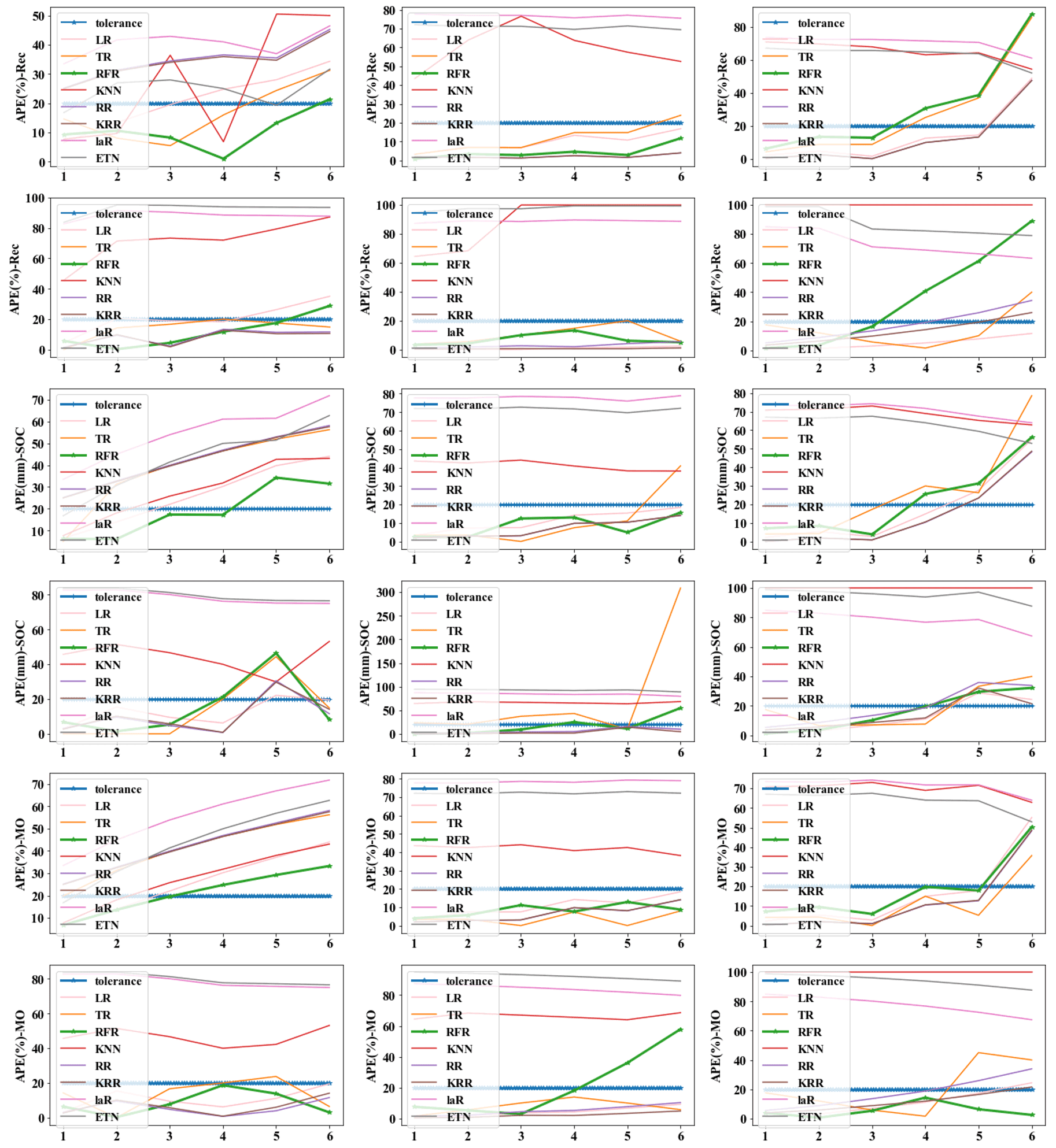
Figure A3 Absolute percent error (APE) of different strategies. (The x axis represents predicted steps within each group.)