the Creative Commons Attribution 4.0 License.
the Creative Commons Attribution 4.0 License.
 | 14 Feb 2022
Evaluation of filtering methods for use on high-frequency measurements of landslide displacements
Michael T. Hendry
Renato Macciotta
Trevor Evans
Displacement monitoring is a critical control for risks associated with potentially sudden slope failures. Instrument measurements are, however, obscured by the presence of scatter. Data filtering methods aim to reduce the scatter and therefore enhance the performance of early warning systems (EWSs). The effectiveness of EWSs depends on the lag time between the onset of acceleration and its detection by the monitoring system such that a timely warning is issued for the implementation of consequence mitigation strategies. This paper evaluates the performance of three filtering methods (simple moving average, Gaussian-weighted moving average, and Savitzky–Golay) and considers their comparative advantages and disadvantages. The evaluation utilized six levels of randomly generated scatter on synthetic data, as well as high-frequency global navigation satellite system (GNSS) displacement measurements at the Ten-mile landslide in British Columbia, Canada. The simple moving average method exhibited significant disadvantages compared to the Gaussian-weighted moving average and Savitzky–Golay approaches. This paper presents a framework to evaluate the adequacy of different algorithms for minimizing monitoring data scatter.
- Article
(9587 KB) - Full-text XML
- BibTeX
- EndNote


Landslides are associated with significant losses in terms of mortality and financial consequences in countries all over the world. In Canada, landslides have cost Canadians approximately USD 10 billion since 1841 (Guthrie, 2013) and more than USD 200 million annually (Clague and Bobrowsky, 2010). Essential infrastructure, such as railways and roads that play vital roles in the Canadian economy, can be exposed to damage if it transverses landslide-prone areas. Attempting to completely prevent landslides is typically infeasible, as stabilizing options and realignment may be cost-prohibitive or lead to environmental damage. This accentuates the significance of adopting strategies that require constant monitoring to mitigate the consequences of sudden landslide collapses (Vaziri et al., 2010; Macciotta and Hendry, 2021).
In recent years, detailed studies have addressed the use of early warning systems (EWSs) as a robust approach to landslide risk management (Intrieri et al., 2012; Thiebes et al., 2014; Atzeni et al., 2015; Hongtao, 2020). The United Nations defines an EWS as “a chain of capacities to provide adequate warning of imminent failure, such that the community and authorities can act accordingly to minimize the consequences associated with failure” (UNISDR, 2009). Although an EWS comprises various components acting interactively, the core of its performance relies on its ability to detect the magnitude and rate of landslide displacement (Intrieri et al., 2012). Given that the timely response of an EWS determines its effectiveness, an accurate sense of landslide velocity and acceleration is necessary. Monitoring instruments able to provide real-time or near-real-time readings such as global navigation satellite systems (GNSSs) and some remote sensing techniques are satisfactory for this purpose (Yin et al., 2010; Tofani et al., 2013; Benoit et al., 2015; Macciotta et al., 2016; Casagli et al., 2017; Chae et al., 2017; Rodriguez et al., 2017, 2018, 2020; Huntley et al., 2017; Intrieri et al., 2018; Journault et al., 2018; Carlà et al., 2019; Deane, 2020; Woods et al., 2020, 2021). These instruments can record the displacement of locations at the surface of the landslide with a high temporal resolution, which allows the monitoring system to track movements on the order of a few millimeters per year. In practice, the results are usually obscured by the presence of scatter, also known as noise, and outliers that affect the quality of observations. These unfavourable interferences do not reflect the true behaviour of the ground motion and stem from sources such as the external environment and the quality of the communication signals and wave propagation in the case of remote sensing techniques (Wang, 2011; Carlà et al., 2017b).
Scatter can be defined as measurement data that are distributed around the “true” displacement trend such that the average difference between the scatter and the displacement trend is zero and has a finite standard deviation. Scatter in displacement measurements can significantly impact the evaluation of slope movements performed on unfiltered data and decrease the reliability of an EWS. This can lead to false warnings of slope acceleration or unacceptable time lags between the onset of slope failure and its identification and therefore a loss of credibility for an EWS (Lacasse and Nadim, 2009). As a result, scatter should be reduced as much as possible without removing the true slope displacement trends. The application of algorithms that work as filters aims to minimize the amplitude of measured scatter around the displacement trend.
Several approaches have been proposed to filter displacement measurements based on either the frequency or time domain. Fourier and wavelet transformations aim to find the frequency characteristics of the data and then attenuate or amplify certain frequencies. These approaches are discussed in Karl (1989), who suggests they are generally unsuitable for non-stationary data such as monitoring data time series. Filters that work on the time domain can be classified as recursive, kernel, or regression filters. Recursive filters, such as the exponential filtering function, calculate the filtered value at a given time based on the previous filtered value. Kernel filters, which include simple moving average (SMA) and Gaussian-weighted moving average (GWMA), calculate the filtered values as the weighted average of neighbouring measurements. Of these two kernel filters, SMA is frequently used in the literature largely due to its simplicity (Dick et al., 2015; Macciotta et al., 2016, 2017b; Carlà et al., 2017a, b, 2018, 2019; Bozzano et al., 2018; Intrieri et al., 2018; Kothari and Momayez, 2018; Chen and Jiang, 2020; Zhou et al., 2020; Desrues et al., 2022; Grebby et al., 2021; Y. H. Zhang et al., 2021; Y. G. Zhang et al., 2021). Regression filters calculate the filtered values by means of regression analysis on unfiltered values (e.g., Savitzky–Golay, or S-G) (Savitzky and Golay, 1964; William, 1979; Cleveland, 1981; Cleveland and Devlin, 1988; Reid et al., 2021). Carlà et al. (2017b) studied both SMA and exponential filtering on multiple failed landslide cases and concluded the latter is inferior in terms of accuracy of failure time prediction. On the other hand, Carri et al. (2021) cautioned the designers and users of EWSs against the use of SMA when rapid movements are expected. However, published applications of filters other than SMA for landslide monitoring are scarce, and studies dedicated to comparing the functionality of other filters to that of SMA are limited.
This paper presents an approach to detect and remove outliers, evaluates the performance of three filters (SMA, GWMA, and S-G), and assesses their suitability to be utilized in an EWS. We evaluated three filters against the following criteria: (1) scatter is minimized, (2) true underlying displacement trends are kept with as little modification as possible, and (3) filtered displacement trends detect acceleration episodes in a timely manner. Moreover, the paper investigates the significance of the time lag between a landslide acceleration event and its identification by a monitoring system for the three filters evaluated.
2.1 Synthetic data generation
A numerical analysis on a synthetic dataset approach was adopted, which consists of synthetic dataset scenarios generated to resemble typical landslide displacement measurements, including acceleration and deceleration periods. These scenarios are idealizations based on observations of typical landslide displacements published in the literature (Leroueil, 2001; Intrieri et al., 2012; Macciotta et al., 2016; Schafer, 2016; Carlà et al., 2017a; Scoppettuolo et al., 2020). A total of 12 dimensionless scenarios were built, with all data between the coordinates x=0, y=0 and x=1, y=1. The x value represents time, and normalization between 0 and 1 allows for extrapolation of the findings for variable displacement measurement frequencies (e.g., the full range of x could represent a week, a month, a year). The analysis of synthetic data focuses on the ability of different algorithms to minimize scatter and identify changes in measured trends; therefore, y represents any of the displacement measurement metrics of interest (displacement, cumulative displacement, velocity, inverse velocity, etc.). Mathematical equations and graphical illustrations of the 12 scenarios are shown in Fig. 1.
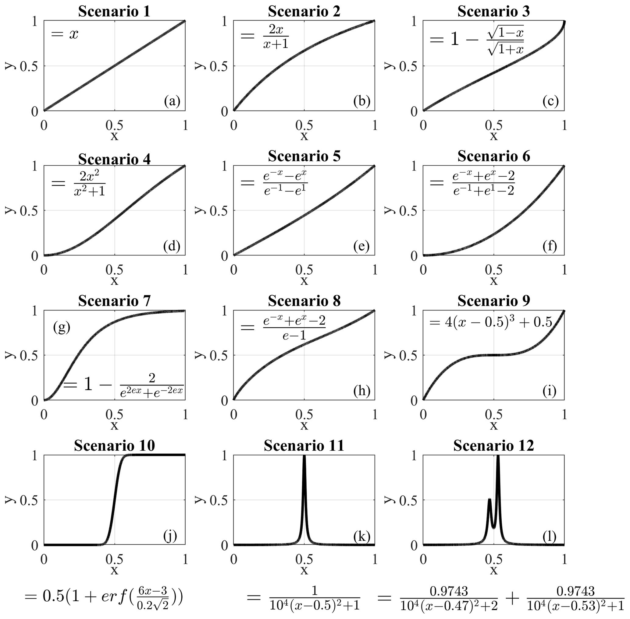
Table 1Number of points used to generate scenarios and examples of their corresponding time spans represented by the range of x from 0 to 1 if the measurement frequency is known (1 h and 1 m readings for illustrative purposes).

The first nine scenarios are referred to as harmonic scenarios, which are characterized by gradual changes in the trend of parameter y. The remaining three scenarios show sudden variations at or near x=0.5 and are referred to as instantaneous scenarios. Considering the discrete nature of instrument measurements, and to account for different ranges in measurement frequencies, each scenario was generated several times, each time with a different number of points (Table 1).
The next step was adding random scatter to the scenarios to represent unfiltered displacement measurements. Macciotta et al. (2016) show the scatter in displacement monitoring for a GNSS used in their analyses fitted a Gaussian distribution. We validated that the scatter distribution fit approximates a Gaussian distribution for the displacement data scatter of the case study in this paper. This assumption, however, has an underpinning theoretical base established by the central limit theorem in probability theory. It states that the mathematical summation of independent variables (such as scatter) goes toward a Gaussian distribution (Smith, 2013). As a result, the scatter was randomly produced from a normal distribution centered at 0, with extreme values truncated between −1 and 1 and a standard deviation of 0.20. Random generation of the scatter followed the techniques outlined in Clifford (1994) known as the acceptance–rejection method, which generates scatter values through a series of iterations until the algorithm generates the initial normal distribution. The amplitude of the scatter around the trend in parameter y was defined for each scenario by scaling the randomly generated scatter. This allowed for the investigation of the effect of different scatter magnitudes on the performance of the filters. Scaling was done by defining the ratio , which is the ratio of scatter amplitude (maximum deviation around the trend, termed n) to the range of values of the trend (t) in each scenario. Six levels of (0.001, 0.005, 0.010, 0.050, 0.100, and 0.150) were considered when performing the analysis to cover a range of possible levels of scatter in unfiltered measurements. Figure 2 shows two samples of synthetic unfiltered scenarios that are the result of superimposing scatter with values of 0.05 and 0.10 on scenario no. 7.
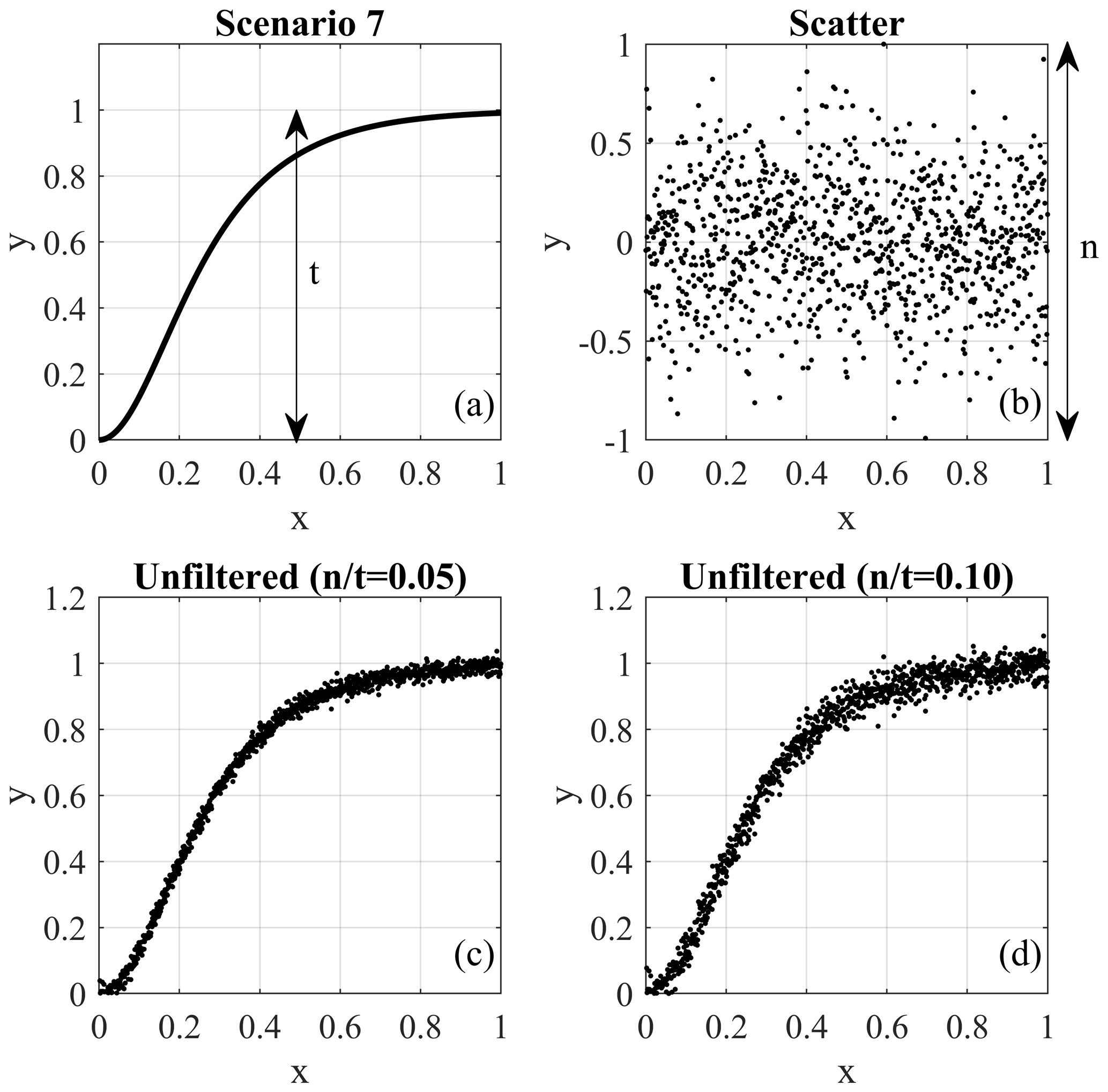
Figure 2The procedure of generating a scenario with scatter: (a) generated scenario trend, (b) randomly generated scatter, and two scenarios with scatter based on values of (c) 0.05 and (d) 0.10.
2.2 Data processing approaches
2.2.1 Simple moving average
SMA is a well-known method for scatter reduction that attempts to reduce scatter by calculating the arithmetic mean of neighbouring points' values. A constant-length interval (window or bandwidth) is used for the calculation for each point; this is also termed a “running” average. Equation (1) is the formulation of this method, which was used by Macciotta et al. (2016) to analyze GNSS data scatter:
where is the filtered value, yj is the unfiltered value, and p is the window length. The window length is constant across the dataset except for regions near the boundaries where fewer points are available. Accordingly, p will be adjusted to the number of available points that are indeed less than the value set by the user. This will cause variation in the effectiveness of the method at the extremes, which needs to be considered when evaluating the results of this approach.
2.2.2 Gaussian-weighted moving average
Varying the weights of the measurements within the calculation window in SMA can be used to develop different filtering methods. The largest weight can be given to the measurement at the time for which the calculation is being done, with weights decreasing for measurements farther away in time. One simple weighting function that can be adopted is the Gaussian (normal) distribution. Equation (2) is the formulation of the Gaussian-weighted moving average (GWMA):
where wj is the weight coefficient based on the Gaussian distribution, and the other terms follow the same definition as per SMA.
2.2.3 Savitkzy–Golay
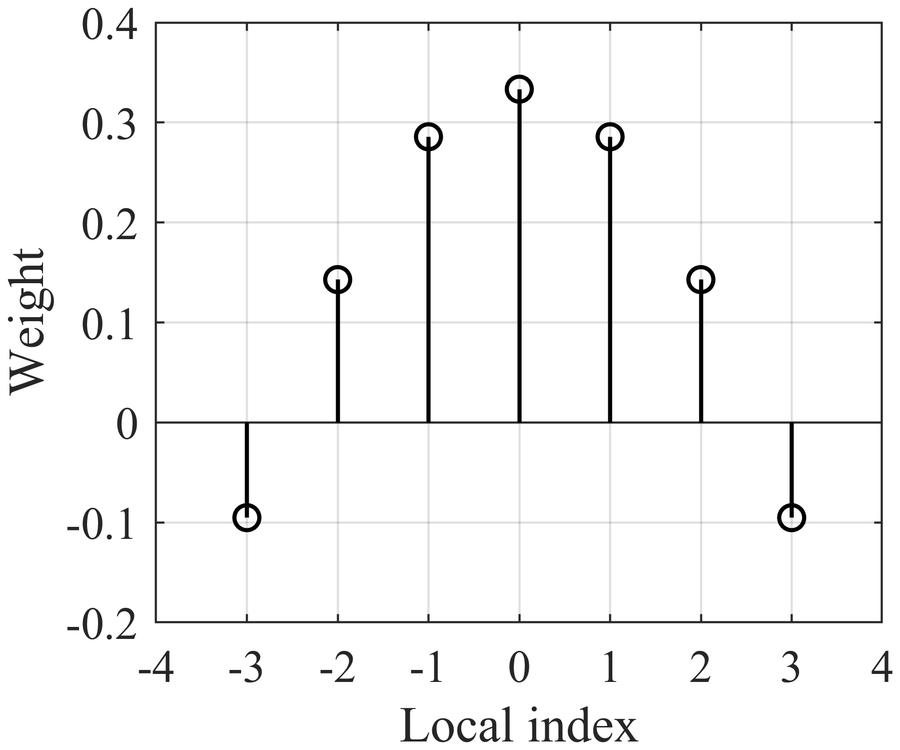
S-G fits a low-degree polynomial equation to the unfiltered measurements within a window and defines the filtered measurements using the fitted curve (Schafer, 2011). Although this procedure seems dissimilar to the weighted averaging as discussed for GWMA, its function can be transformed into a kernel concept using the least-squares method if the data points are evenly spaced. The detailed procedure is presented in Appendix A. Figure 3 shows the weight kernel over a window of seven points attained by fitting a quadratic polynomial. An immediate observation is that some points are given negative weights. If points are not evenly spaced, the weighting kernel cannot be used, and local regression analysis should be periodically conducted for each point. Such filtering is known as locally estimated scatterplot smoothing (LOESS). This decreases the computational efficiency of filter performance and exponentially increases the execution time.
2.3 Evaluation of processing algorithms
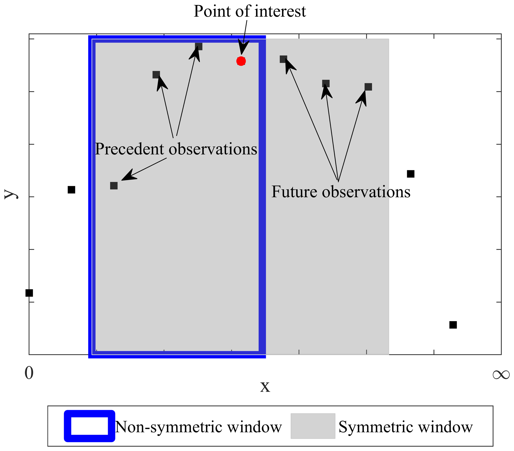
The synthetic monitoring data and data from the case studies were filtered using SMA, GWMA, and S-G techniques. The filters were applied with different lengths of moving windows, from 0.01 (1 %) to 0.1 (10 %) of all monitoring points, referred to as the bandwidth ratio. These limits for the bandwidth ratio were selected based on literature reports for SMA. In the filtration process, we only used the points prior to the time for which the calculation is being made (point of interest, Fig. 4). This is to reflect the reality of displacement monitoring information as applied to EWSs. To this end, filters used the first half of their kernels, but the weights were multiplied by 2 in comparison to a symmetric window in order to keep the sum of weights equal to 1.
All of these filters require the definition of the bandwidth. A roughness factor was defined to aid in the evaluation of the effect of bandwidth in reducing scatter. This factor is defined as follows:
where J2 is the roughness factor, is the second derivative of filtered measurements, Ra is the absolute roughness computed by Eq. (4), and y′′ is the second derivative of unfiltered measurements. The second derivative measures how much the slope of the line connecting two consecutive points changes, which itself is an indication of fluctuation. The greater this second derivative, the greater the variation. J2 was normalized to the overall curvature of the unfiltered scenario to determine the relative scatter reduction after the application of a filter, eliminating any roughness associated with the real trend in the scenario. In limit states, a value of 1 means that fluctuations are similar to the unfiltered dataset, and therefore no improvement has been achieved; a value of 0 suggests the slope of a scenario remains unchanged and indicates a linear trend. Because all the scenarios, except the first, include trends showing concavity or convexity, a residual value for the roughness factor would be expected in the lowest limit state, meaning that a value of 0 is not necessarily a goal. J2 was used to infer the minimum value of bandwidth ratio after which no significant change in the fluctuation of results is achieved. Considering the second power in the formulation of J2, all observations are valid if the scenarios are mirrored (when they vary from 1 to 0, instead of 0 to 1).
The filters are not expected to remove all scatter, and the error attributed to the residual scatter can be calculated using the root mean square error (RMSE). Given that velocity values are usually used as thresholds in an EWS, one concern is whether the filter should be applied to displacement values or velocity values derived from unfiltered displacements. To address this issue, two different approaches to filtering were investigated: direct and indirect. As a result, two different approaches using the RMSE were also utilized here.
2.3.1 Direct scatter filtration
Direct filtration means the filter is applied to the diagram of interest. If the filtered displacement values are the goal, and the filter is applied to unfiltered displacement values, then the filtering process is called direct filtration. The same concept applies when velocity values are derived using unfiltered displacements, and the filters are then directly applied to the velocity values. In this approach, the RMSE follows Eq. (5):
where RMSEd is the measurement of error in direct filtration, yi is the value of the true trend (for the synthetic scenario), is the filtered value, and m is the total number of points. This approach is often used in the literature (e.g., Macciotta et al., 2016; Carlà et al., 2017a,b, 2018, 2019; Intrieri et al., 2018).
2.3.2 Indirect scatter filtration
Some EWSs can apply the filter to the displacements but use velocity trends as the metric for evaluation. In this case, the filtered velocity values will be computed using the filtered displacements. Indirect filtration indicates the diagram of interest is the first derivative of the diagram to which the filter is applied. The RMSE, in this case, is defined as follows:
where RMSEi is the measurement of error in indirect filtration, is the first derivative of the true trend, is the first derivative of filtered data (derived velocity after the filter is applied to the displacements), and m is the total number of points. Similar to J2, all observations are valid for the mirrored scenarios of those presented in Fig. 1. This is a consequence of using the second power in the definition of RMSEi and RMSEd.
2.4 Lag quantification
Only antecedent measurements are fed into the filters, which is expected to result in a lag between the true trend and its identification by the filters. This lag means the calculated value of velocity or displacement occurred sometime in the past. Consequently, reducing this lag means less time is lost with respect to providing an early warning. To quantify the induced lag, the filtered diagrams of all scenarios at all ratios and bandwidth ratio values were shifted backwards a number of points equivalent to 0.001 (0.1 %) to 0.1 (10 %) of all generated points. We refer to this as the shift ratio in the rest of this paper. This shift of filtered diagrams is expected to increase their similarity with the true trend until the best correlation is achieved. The R2 test was used to determine how well the shifted and filtered results replicate the underlying trend.
2.5 Geocube differential GNSS system
A Geocube system is a network of differential global navigation satellite system (GNSS) units that work with a single frequency (1572.42 MHz), making it cost-effective (Dorberstein, 2011; Benoit et al., 2014; Rodriguez et al., 2018). Geocubes communicate with each other through radio frequency, and a reference unit outside the boundaries of the landslide is assumed as static for differential correction to increase the poor accuracy associated with single frequency GNSSs (Benoit et al., 2014; Rodriguez et al., 2018). The ability of this system to achieve real-time positioning, remote data collection, and processing makes it a suitable candidate for incorporation into an EWS. As a result, Geocube data are used in this study to evaluate the performance of the three mentioned filters.
2.6 Outlier detection
Outliers are defined herein as abnormal inconsistencies (e.g., displacement directions, magnitudes) when compared to the majority of observations in a random sampling of data (Zimek and Filzmoser, 2018). Techniques for outlier detection have been proposed based on the statistical characteristics of datasets. One common example is the Z score method, which calculates the mean and standard deviation of data within a defined interval and identifies outlier data as those beyond 3 standard deviations from the mean (Rousseeuw and Hubert, 2011). A limitation of this kind of approach is the sensitivity of the mean and standard deviation to the outlier data points, which has led to the development of other methods that use other indices such as the median (Salgado et al., 2016). One such technique that was adopted in this study is the Hampel filter (Hampel, 1971). In this method, the median of the displacement measurements within a running bandwidth is calculated, and data outside a defined threshold from the median are identified as outliers. The threshold is defined as a constant (threshold factor) multiplied by the median absolute deviation. An asymmetric window with a bandwidth ratio of 0.004 (0.4 %) and a threshold factor of 3 was adopted following previous studies (Davies and Gather, 1993; Pearson, 2002; Liu et al., 2004; Yao et al., 2019). The data identified as outliers were then removed from the dataset.

Figure 5(a) Location of the Ten-mile landslide (source: Earthstar Geographics LLC) and (b) front view of the Ten-mile landslide and distribution of Geocubes on its surface (Rodriguez et al., 2018; Macciotta et al., 2017b).
The Ten-mile landslide is located in southwestern British Columbia (BC), in the Fraser River Valley north of Lillooet (Fig. 5a). It is a reactivated portion of a post-glacial earthflow (Bovis, 1985) that was first recognized in the 1970s. The landslide velocity has increased from an average of 1 mm d−1 in 2006 to 6 mm d−1 in 2016, with a maximum measured velocity of 10 mm d−1 (Gaib et al., 2012; BGC Engineering Inc., 2016). The movement of this landslide impacts the integrity of BC Highway 99 and a section of railway operated by Canadian National Railway (CN) (Carlà et al., 2018), with most movement limited to the volume downslope from the railway due to the installation of a retaining wall (Macciotta et al., 2017a). Despite the stabilization work done to date, the uppermost tension crack has retrogressed approximately 200 m in 45 years and is now situated 60 m upslope of the railway track (Macciotta et al., 2017b). The landslide lateral extents have not expanded since 1981 according to the aerial photographs (Macciotta et al., 2017b). The Ten-mile landslide is currently approximately 200 m wide, 140 m high, and has a volume of 0.75 to 1 million m3, moving towards the Fraser River on a continuous rupture surface with a dip of about 22 to 24∘, which is sub-parallel to the ground surface (Rodriguez et al., 2017; Donati et al., 2020). The elevation of the shear surface and mechanism of the landslide have been inferred from the readings of multiple slope inclinometers installed in 2015 (BGC Engineering Inc., 2015).
The bedrock in this region consists of volcanic rocks, such as andesite, dacite, and basalt, and is overlain by Quaternary deposits (Donati et al., 2020; Carlà et al., 2018; Macciotta et al., 2017a). The thickness of the landslide varies between 20 and 40 m, and the ground profile from the surface to depth comprises medium to high plastic clays and silts overlying colluvium material and glacial deposits, overlying bedrock (BGC Engineering Inc., 2015). The stratigraphy of the sedimented soils in the landslide area notably varies from one borehole to another and reflects the complex stratigraphy of the earthflow.
A total of 11 Geocubes were installed at the Ten-mile landslide in 2016. Figure 5b is a front view of the landslide showing the locations of the Geocube units. Units 44 and 50 are installed near the uppermost tension crack identified as the current landslide backscarp, unit 69 is 30 m above the backscarp, and unit 39 is used as the reference point. Please note that unit 69 is used as the fixed Geocube and is not shown in Fig. 5b. The other units are located within the boundaries of the landslide, with a maximum distance between units of 310 m (Rodriguez et al., 2018). The time step between every two consecutive measurements is 60 s. Figure 6 shows the displacements of units 46 and 47, which were the largest in comparison to other Geocubes.
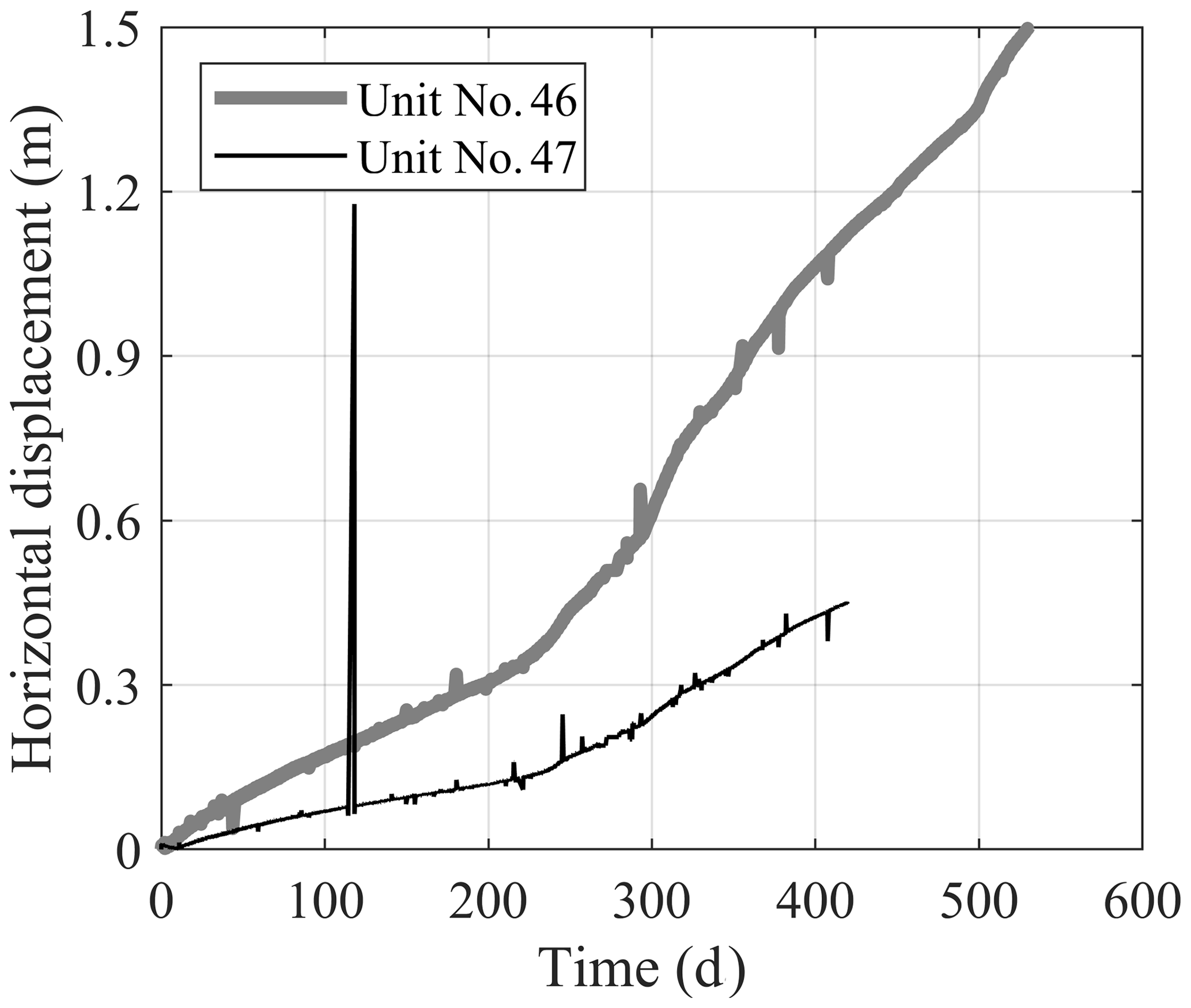
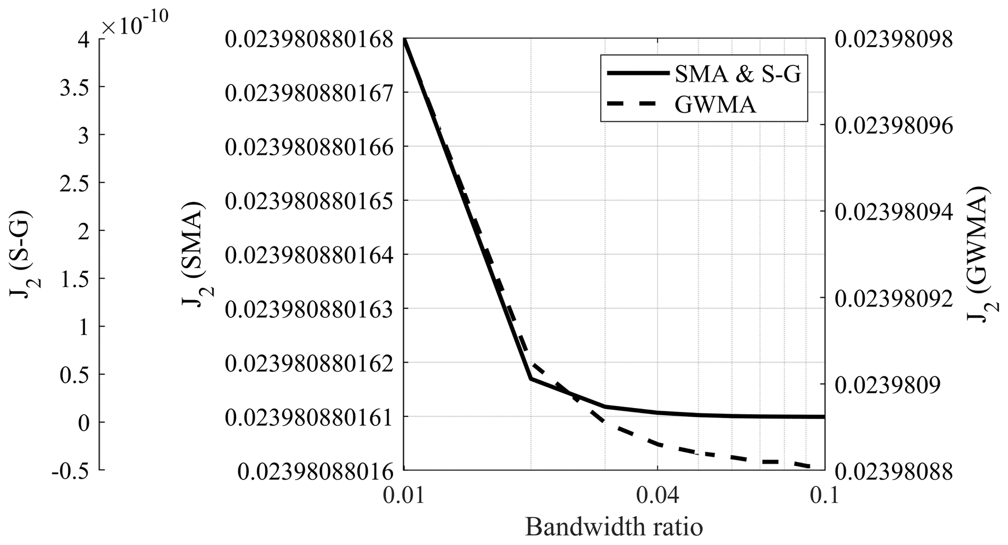
Figure 7Variation in roughness factor for scenario 6 with respect to the applied filter on a semi-log scale.
4.1 Synthetic analysis
Figure 7 shows the roughness value (J2) of scenario 6 for SMA, GWMA, and S-G on a semi-logarithmic scale. This figure illustrates how, regardless of the ratio, J2 substantially decreases as the bandwidth ratio increases to 0.01 and then asymptotically approaches a final value. This means that increasing the bandwidth ratio drastically reduces scatter; however, its effectiveness is restricted as the bandwidth ratio increases above 0.01. This observation was consistent for other scenarios. J2 values (including scenario 6 in Fig. 7) indicate that J2 approaches its minimum at bandwidth ratio values of 0.03 to 0.04, regardless of the filter selected.
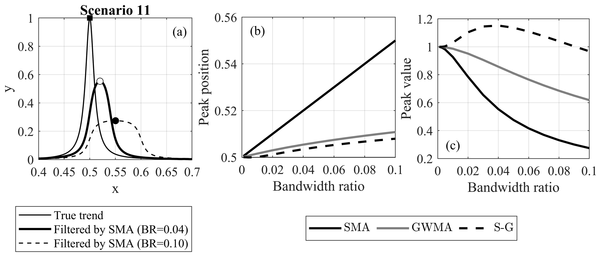
Figure 8(a) An example of peak displacement by applying SMA, as well as variation in (b) peak position and (c) peak value with respect to the filter and bandwidth ratio used (original peak at 0.5).
4.1.1 Effect of filters on trend distortion
Scenarios 11 and 12 were first analyzed to evaluate the degree to which the trend was preserved by these filters as peaks made it easier for visualization. Figure 8a shows the true trend of scenario 11 along with two SMA-filtered scenarios at bandwidth ratios of 0.04 and 0.10, respectively. This figure shows that, as the SMA filter bandwidth increases, the peak in measurements is identified at a later time than the true trend (x=0.5) and the magnitude of the peak is reduced (more than 70 % reduction at a bandwidth ratio of 0.10). Furthermore, as the bandwidth ratio increases, the “instantaneous” nature of the peak is lost to a more transitional variation. This highlights a disadvantage of SMA when handling sudden changes in data trends. The calculated x value of the peak in scenario 11 is plotted for different bandwidth ratios and for all three filters in Fig. 8b. This figure shows the time at which the peak is identified lags as the bandwidth ratio increases for all filters; however, GWMA and S-G identify the peak with a much smaller lag, independent of the ratio. As an example, for a year of monitoring data at a frequency of 30 s and bandwidth ratio of 0.10, SMA, GWMA, and S-G predict the peak point approximately 17, 3.5, and 2.7 d after the real peak, respectively. This lag can be attributed to the utilization of an asymmetric window, which leads to a lagged response of the filter. As more points are included in the filtering procedure (increasing bandwidth ratio), this lag increases because the averaging process is sensitive to window type. The degree of sensitivity, however, depends on the filter. Figure 8c shows the variation in the peak magnitude with respect to the bandwidth ratio for all three filters. SMA and GWMA both underestimate the peak value, and the difference between the calculated peak and real peak increases as the bandwidth ratio increases. SMA calculations underestimate the peak more than twice as much as GWMA. On the contrary, S-G intensifies the peak up to a bandwidth ratio of 0.04, with the impact tending to diminish at larger bandwidth ratios; it predicts the true value at a bandwidth ratio value of almost 0.09.
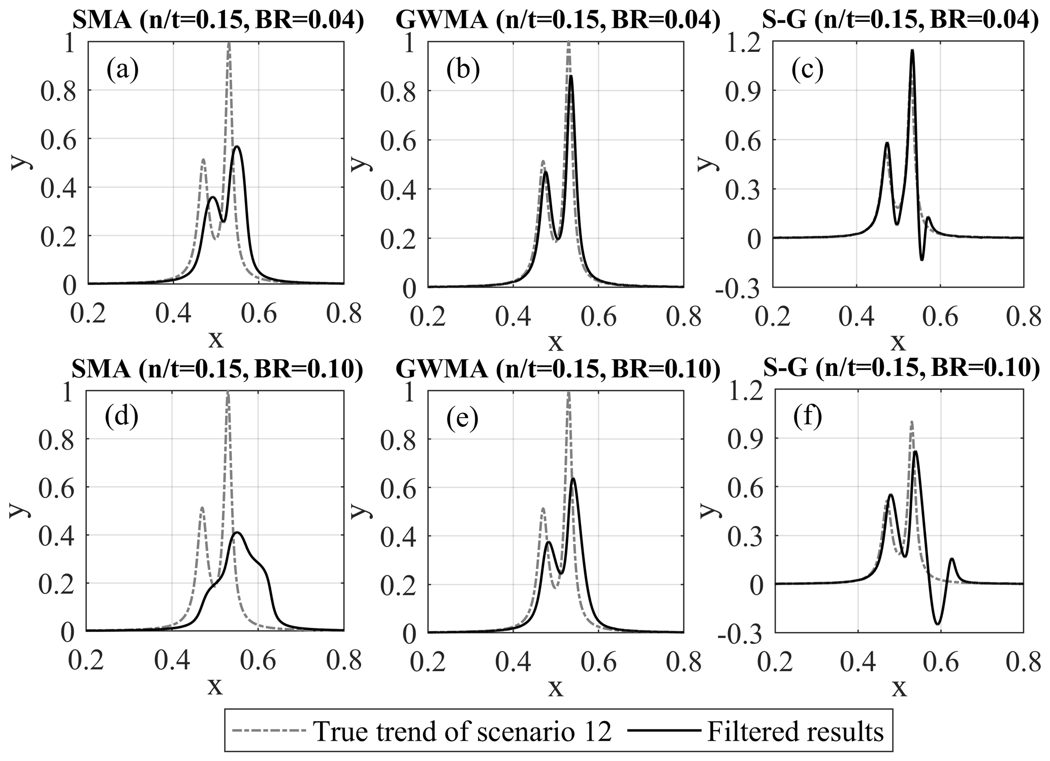
Figure 9Filtered results of Scenario 12 with scatter using SMA (a, d), GWMA (b, e), and S-G (c, f) at bandwidth ratios (BRs) of 0.04 (a–c) and 0.10 (d–f).
Scenario 12 was used for a detailed evaluation of the ability of these filters to conserve the underlying original trend. Figure 9 shows scenario 12 and the filtered results for all three filters and an ratio of 0.15. This scenario and these specific parameters were selected for illustration purposes as they allow visual identification of differences for discussion. The SMA filter considerably underestimates the magnitude of the peak at a bandwidth ratio of 0.04, which should be the minimum bandwidth ratio according to Fig. 7. At a bandwidth ratio of 0.10, the filtered diagram is distorted in comparison to the true trend, and the initial peak is not identified. GWMA at a bandwidth ratio of 0.04 shows less underestimation of the peak magnitude, and a slight lag is visually observed at a bandwidth ratio of 0.10. This indicates the significantly better performance of GWMA over SMA. S-G results for both bandwidth ratios closely identify the time and magnitude of both peaks, indicating yet better performance. However, the peak is artificially intensified at a bandwidth ratio of 0.04, and a significant drop occurs well beyond the true trend immediately after the second peak for both bandwidth ratios (pulsating effect), which was also observed in scenario 11. Increasing the degree of the polynomial fitted as part of the S-G methodology was not completely effective at eliminating this effect. The pulsating effect was also observed when a symmetrical window was utilized and is attributed to the negative weights in the S-G kernel.
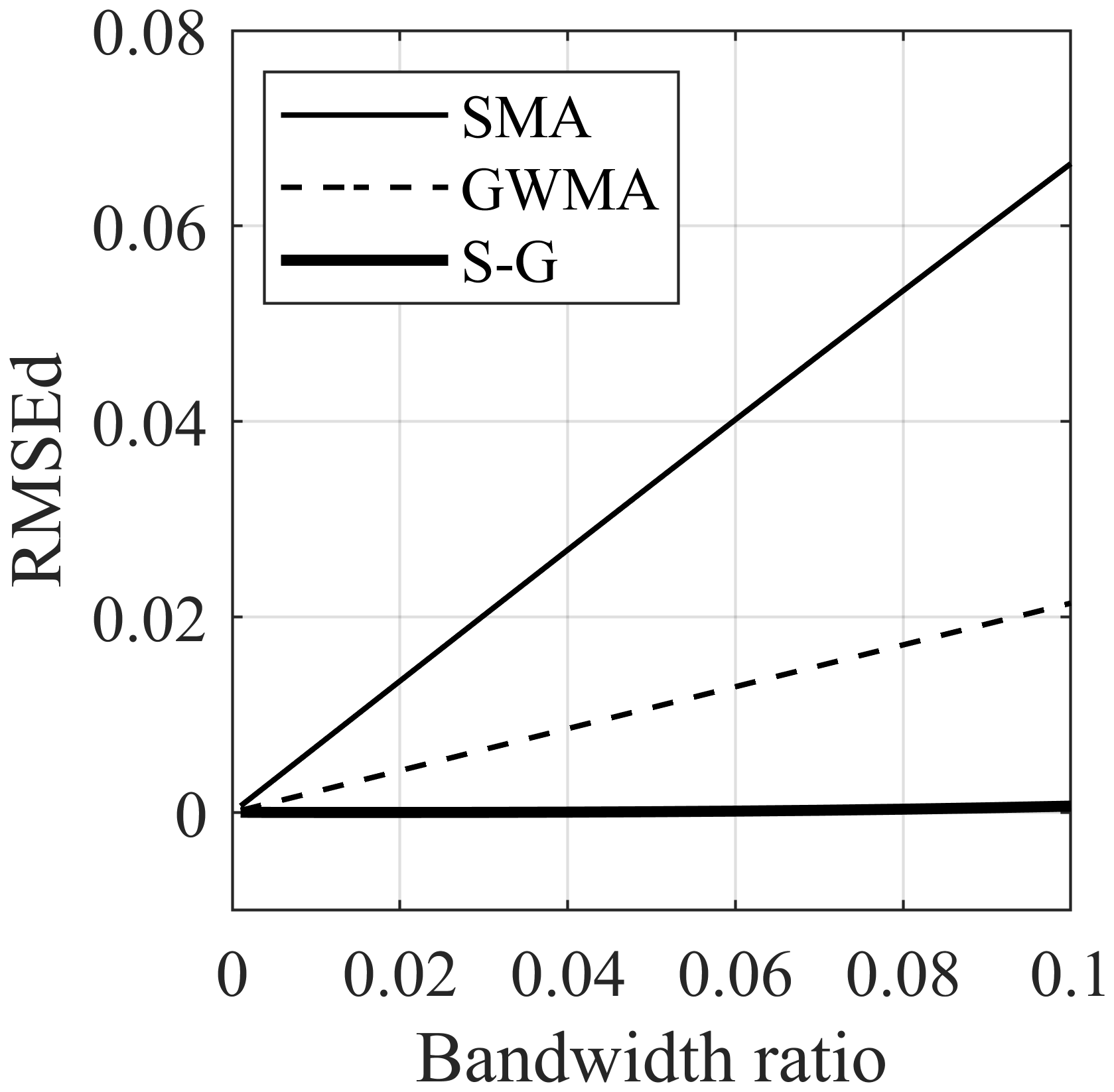
4.1.2 Results of direct scatter filtration
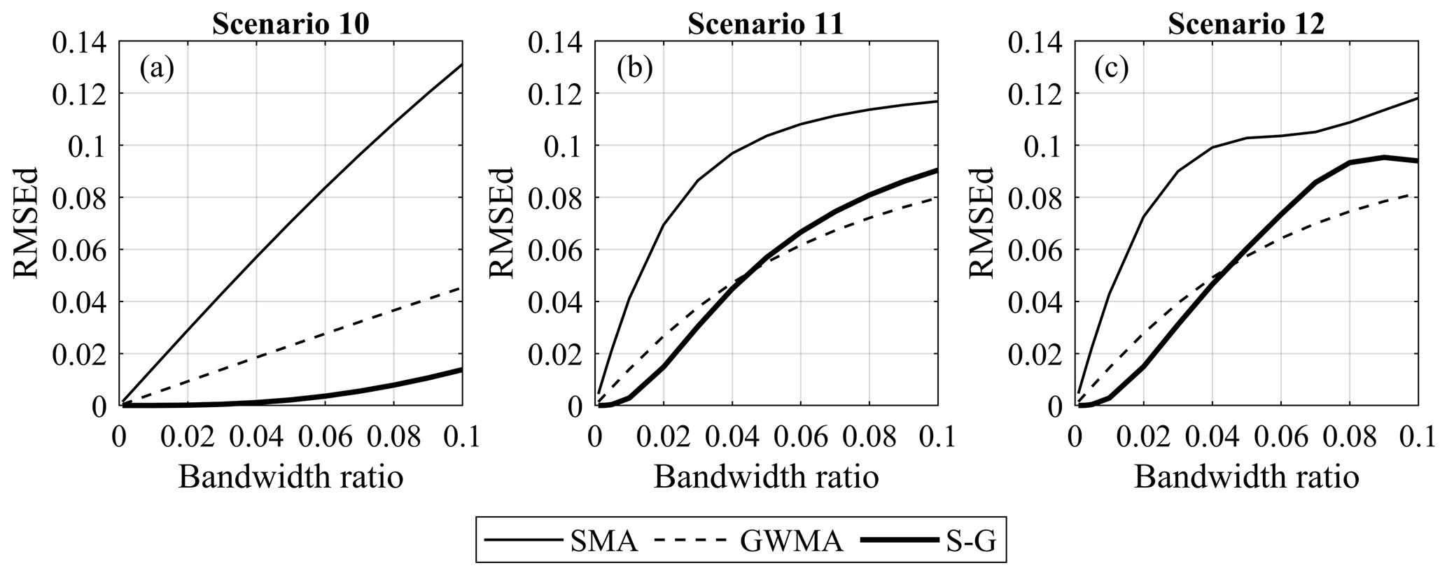
Figure 10 shows the RMSEd of all three filters for all the harmonic synthetic scenarios. This figure shows that, for these numerical analyses on synthetic scenarios, the error depends linearly on the bandwidth ratio for all of the filters and does not depend on the scenario or ratio. SMA shows the greatest difference from the true trend, followed by GWMA (approximately 60 % less difference than SMA). S-G, on the other hand, almost lies on the horizontal axis for all the bandwidth ratios, which means the filtered results yield near-zero error. Figure 10 also shows how the error increases as the bandwidth ratio increases. This can be attributed to the utilization of an asymmetric window, which leads to a lagged response of the filter. As more points are included in the filtering procedure (increasing bandwidth ratio), this lag increases and, consequently, causes a larger error. The RMSEd values of filters for the instantaneous synthetic scenarios are shown in Fig. 11. In scenario 10, the same behaviour as noted for the harmonic scenarios can be seen for SMA and GWMA, whereas S-G is not as accurate. This is more noticeable in scenarios 11 and 12 in which S-G becomes less accurate than GWMA at larger bandwidth ratios. This result shows that S-G cannot handle the instantaneous scenarios as satisfactorily as the harmonic ones. The errors related to SMA and GWMA for the instantaneous synthetic scenarios show non-linear behaviour and are greater when compared to the harmonic scenarios. Figure 11 clearly shows all filters are challenged by the instantaneous variations when compared to gradual ones in direct filtration.
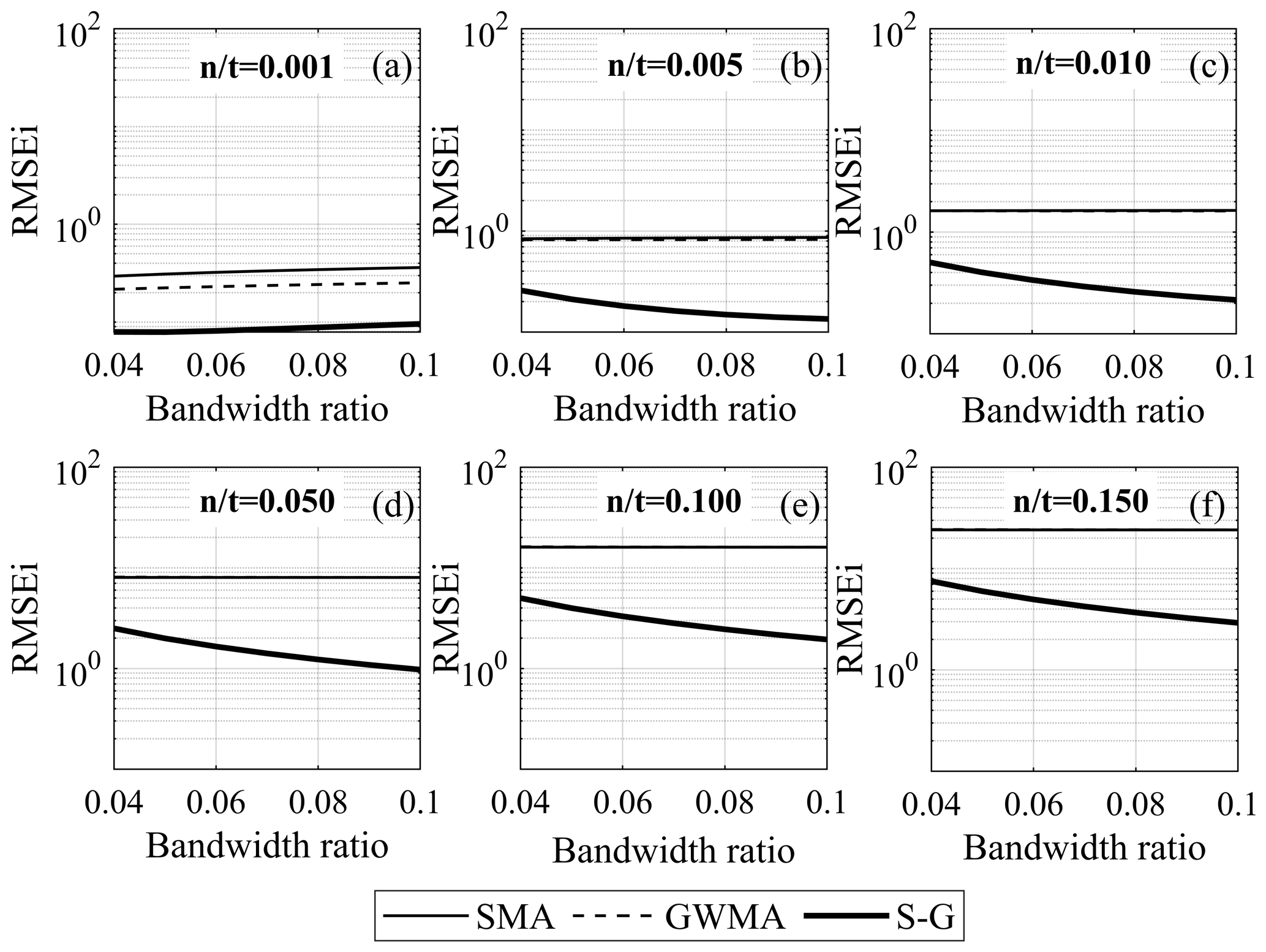
4.1.3 Results of indirect scatter filtration
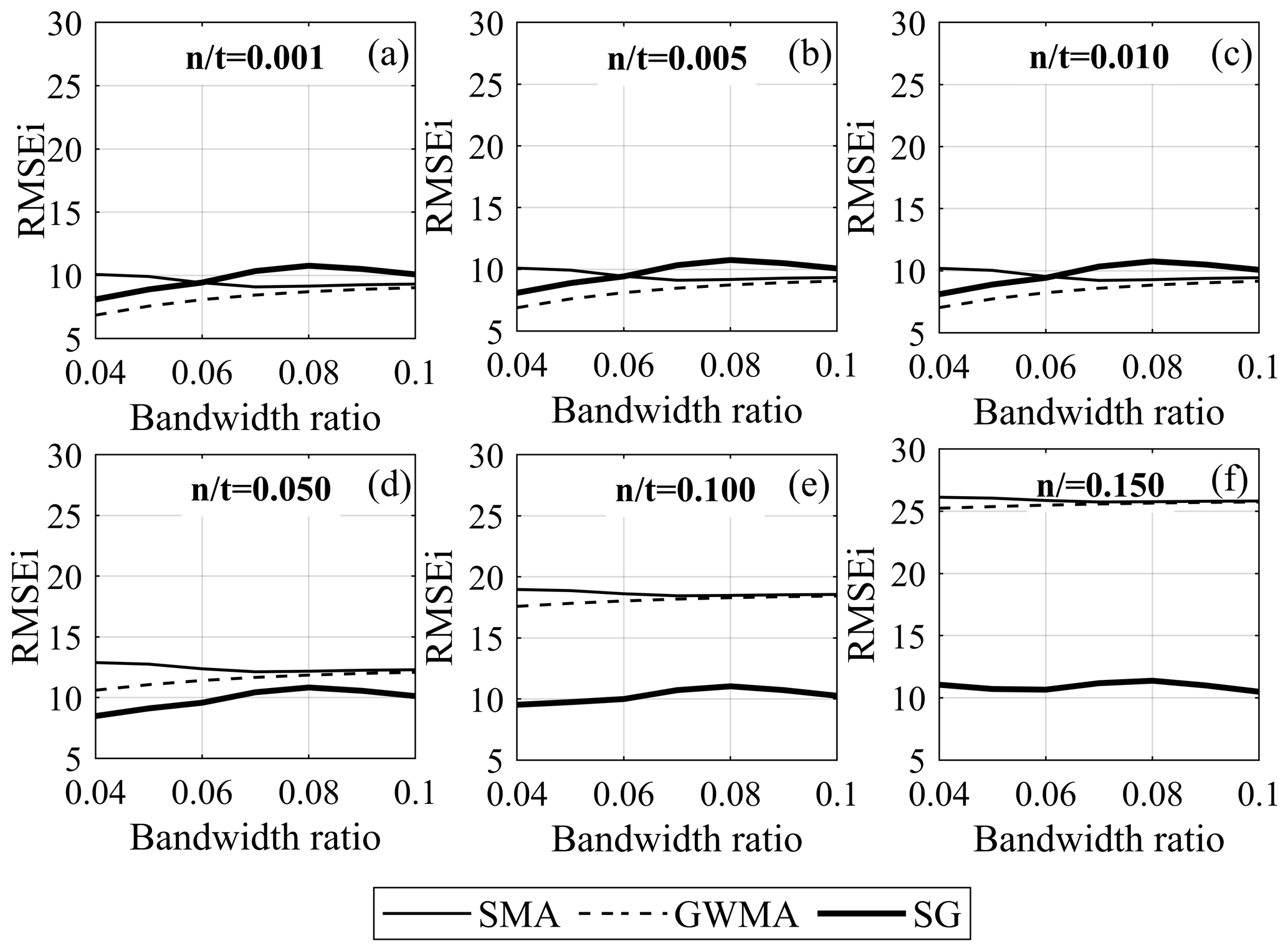
Figure 12 shows the RMSEi results for the harmonic scenarios (when performing indirect filtration) on a semi-logarithmic scale. We observed that the error considerably decreases as the bandwidth ratio increases to 0.02; however, to highlight the variation of error in the range of interest for the bandwidth ratio, only RMSEi values corresponding to bandwidth ratios greater than 0.04 are plotted in Figs. 12 and 13. In Fig. 12, the error for the GWMA is either equal to or slightly less than the error for the SMA, and S-G shows the least error for the harmonic scenarios. The RMSEi results for the instantaneous scenarios (Fig. 13) are similar to those for the harmonic scenarios for large ratios (0.05, 0.10, and 0.15). For small ratios, the GWMA is superior at bandwidth ratios above 0.06, and S-G has the worst performance.
4.1.4 Lag quantification
The non-symmetric inclusion of points causes the identification of a lag in the trend of filtered data. Figure 14 shows Scenario 10 with respect to the original trend, with scatter added (at an value of 0.15), and the results after filtering with each of the three methods at a bandwidth ratio of 0.04. This figure clearly shows the lag between the results filtered by SMA and GWMA and the true trend. S-G results do not have as severe a lag as that resulting from the other filters; we attribute this to the negative weights in its kernel that anchor the filtered values and prevent a lagged response. A minor pulsating effect can be observed in the S-G filtered data, decreasing the calculated values at a much earlier time than the true trend. This suggests that S-G is robust with respect to identifying initial changes in monitoring trends but overcorrects subsequent changes; SMA grossly lags with respect to the identification of any change, and GWMA has a reduced lag when compared to SMA.
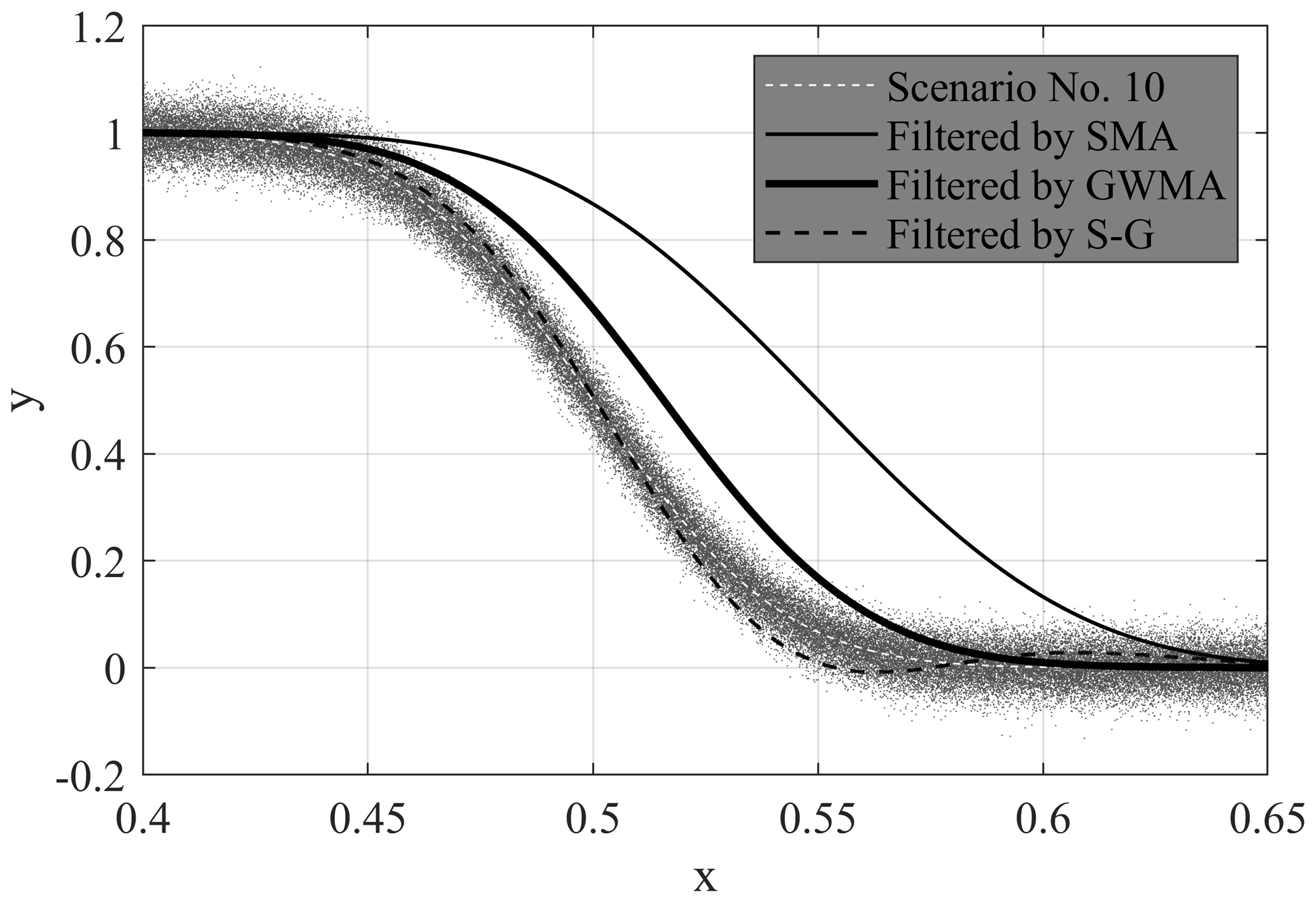
Figure 14Scenario 10 with and without scatter, as well as with scattered results filtered by SMA, GWMA, and S-G for an value of 0.15 and a bandwidth ratio of 0.04.
Figure 15a shows an example of the R2 correlation for scenario 7, comparing the original trend and the results filtered by SMA at an value of 0.01 and bandwidth ratio of 0.04. The shift ratio is the shift of filtered trends (on the horizontal axis – parameter x) relative to the range of x values. R2 calculations are shown for the filtered data (shift ratio of 0) and as the filtered trends are shifted backwards in time (negative shift ratio values). In this analysis, the peak R2 value (largest correlation between the shifted filtered results and original trend) indicates the shift required to minimize the lag in identifying the original trend changes, therefore providing a quantitative approach to calculating the lag in parameter x. In the example in Fig. 15a, the lag corresponded to 0.018 (1.8 %) of the total points.
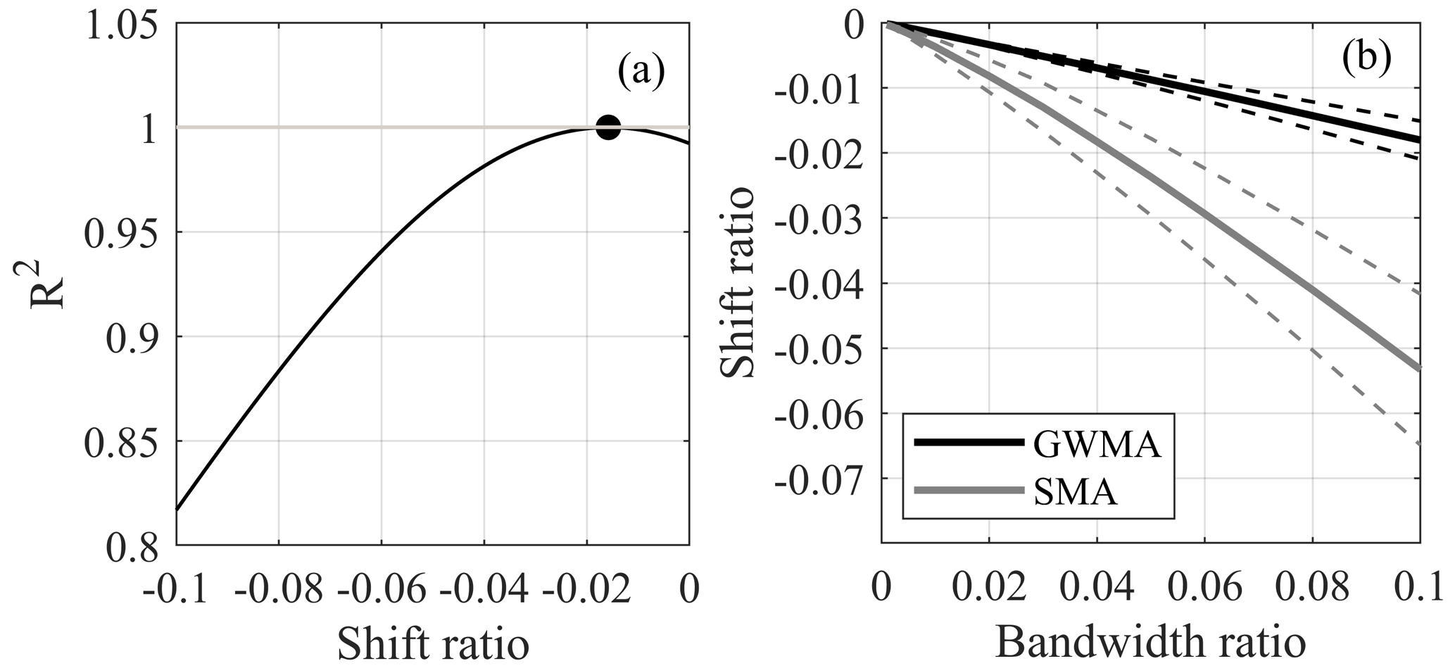
Figure 15(a) R2 values for scenario 7 with filtered and shifted results at an value of 0.01 and bandwidth ratio of 0.04 and (b) shift ratio at peak R2 for all scenarios and ratios, with the mean (solid line) bounded by 1 standard deviation (dashed lines)
Table 2Regression correlations between shift ratio (SR) and bandwidth ratio (BR) with the strength of the correlation in terms of R2 and RMSE.
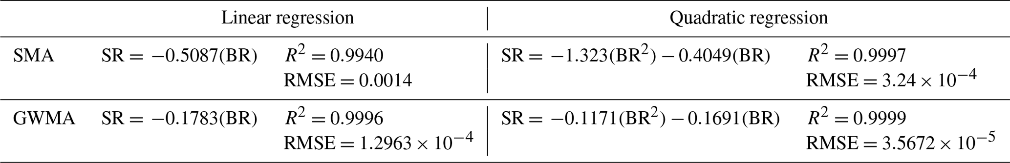
Peak R2 values for all scenarios and values are closely correlated with the bandwidth ratio. The lag, quantified by the shift ratio, is larger when the trend change is more pronounced; therefore, the correlation between the shift ratio and bandwidth ratio is different for different scenarios. Figure 15b shows the mean correlation between the shift ratio and bandwidth ratio, for all scenarios and values, bounded by 1 standard deviation, for GWMA and SMA. Table 2 shows linear and quadratic regressions of this correlation and the strength of the correlation in terms of R2 and RMSE. Figure 15b quantitatively shows that GWMA lags less than SMA with respect to identifying changes in measurement trends. Moreover, the uncertainty associated with lag for SMA is greater than for GWMA because of the larger standard deviation. Figure 15b quantifies how increasing the bandwidth ratio increases the lag with respect to identifying true measurement trends, and, although large bandwidth ratios decrease the scatter in data, the bandwidth ratio should carefully balance minimizing both scatter (J2) and lag (shift ratio). S-G is not included in this analysis as the method resulted in no significant lag in identifying changes in measurement trends; however, it had the disadvantages previously noted including pulsating effects and overestimating peak values.
4.2 Results on the Ten-mile landslide
Unfiltered results reported by Geocubes 46 and 47 installed on the Ten-mile landslide were processed by all three filters. To illustrate to the reader through visual inspection the difference between the performance of SMA, GWMA, and S-G, only a 200 d window of displacement data from Geocube 46 and filtered points produced by direct filtration are shown in Fig. 16. Figure 16a also features an inset showing scaled scenario 4, which resembles the general trend of Geocube 46 data for the period from day 200 to 400. Figure 16 shows that increasing the bandwidth ratio reduces the scatter but increases the lag in the filtered results, consistent with observations on the synthetic datasets. For bandwidth ratios larger than 0.04, SMA becomes insensitive to some short-scale (20 to 30 d) trends in the data (qualitative visual inspection). As an example, at a bandwidth ratio of 0.10, SMA suggests the displacement of Geocube 46 follows a bi-linear trend with an inflection point at day 240, while unfiltered points and other filters suggest other periods of acceleration and deceleration. Importantly, S-G is sensitive to even subtle variation and does not show significant lag.
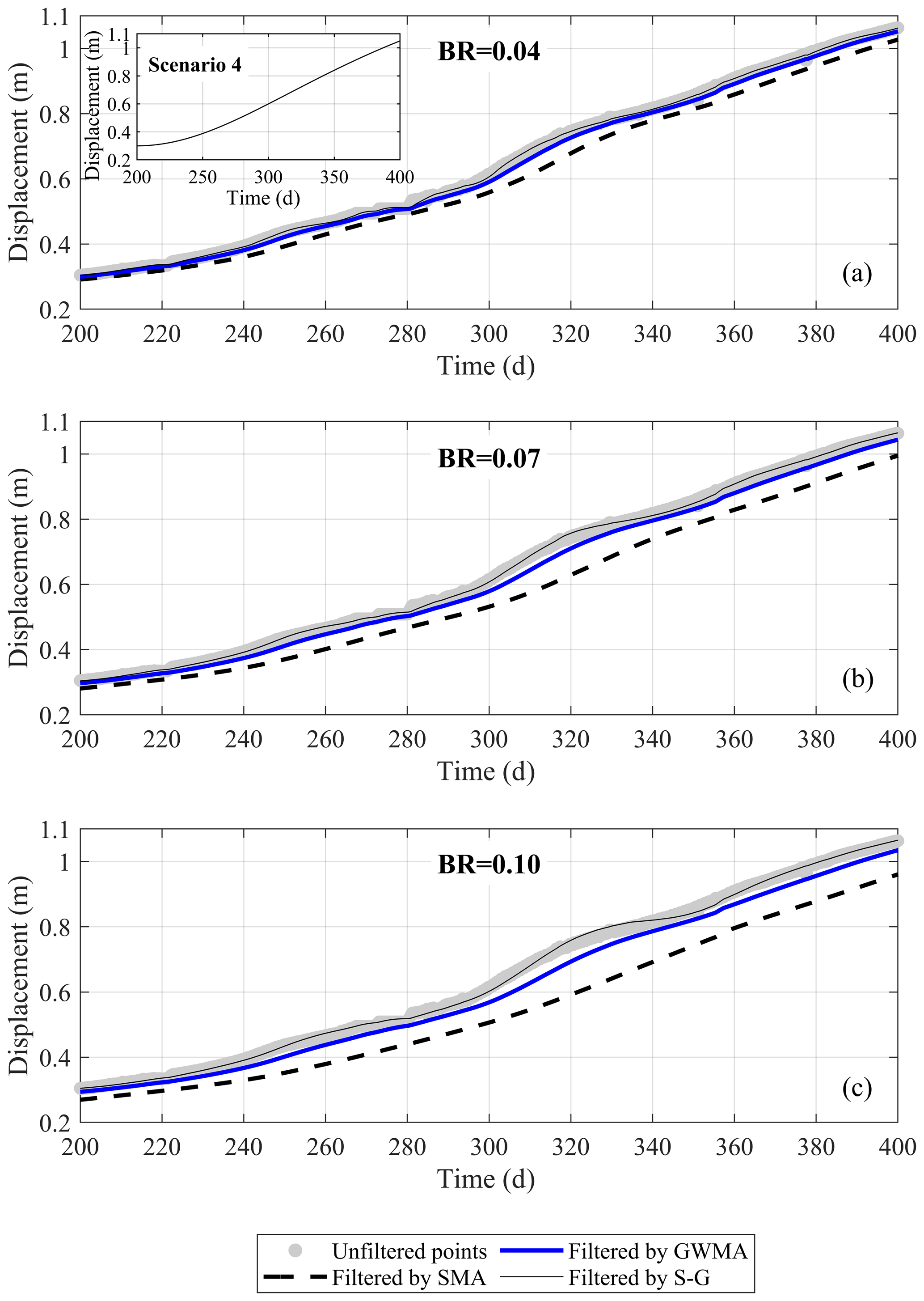
Figure 16Unfiltered displacement of Geocube 46 data vs. time and data filtered by SMA, GWMA, and S-G for bandwidth ratios (BRs) of (a) 0.04, (b) 0.07, and (c) 0.10.
Figure 17 shows the filtered velocity values obtained by directly filtering the calculated velocities and by indirectly filtering the displacement values before calculating the velocity from Geocube 46 data. The direct and indirect filtering approaches demonstrated similar performance in terms of scatter reduction for Geocube 46 data. As the bandwidth ratio increases, SMA tends to significantly attenuate the local maximum and minimum points in comparison to results at smaller bandwidth ratios, indicating a probable loss of information about the landslide behaviour and sensitivity of this filter to the bandwidth ratio, as also noted in Fig. 16 (curvature loss in SMA results). Indirect filtration by SMA seems to be limited near the boundary at time zero, resulting in a subdued replica of direct filtration. The length of this region is found to be governed by the bandwidth ratio, as the necessary number of points for filtering in this portion has not been provided to the filter. This is also observed in S-G results. This problem was not found in GWMA results as direct and indirect filtration both follow the same pattern. GWMA and S-G are both able to preserve the velocity variation even at the most intense filtration (bandwidth ratio of 0.10); however, variations between local maxima and minima are more extreme in S-G than GWMA results. This is attributed to peak overestimation (Figs. 8 and 9) or a pulsating effect superimposing on the peaks/troughs. Moreover, the S-G results still demonstrate relatively large fluctuations even at the largest bandwidth ratio. This means that the application of S-G might still trigger false alarms in an EWS if the landslide is moving at a faster rate or experiencing different episodes of acceleration and deceleration. To avoid this, a larger bandwidth ratio should be used, but this can be problematic due to the higher computational effort required and issues that might follow, such as the pulsating effect.
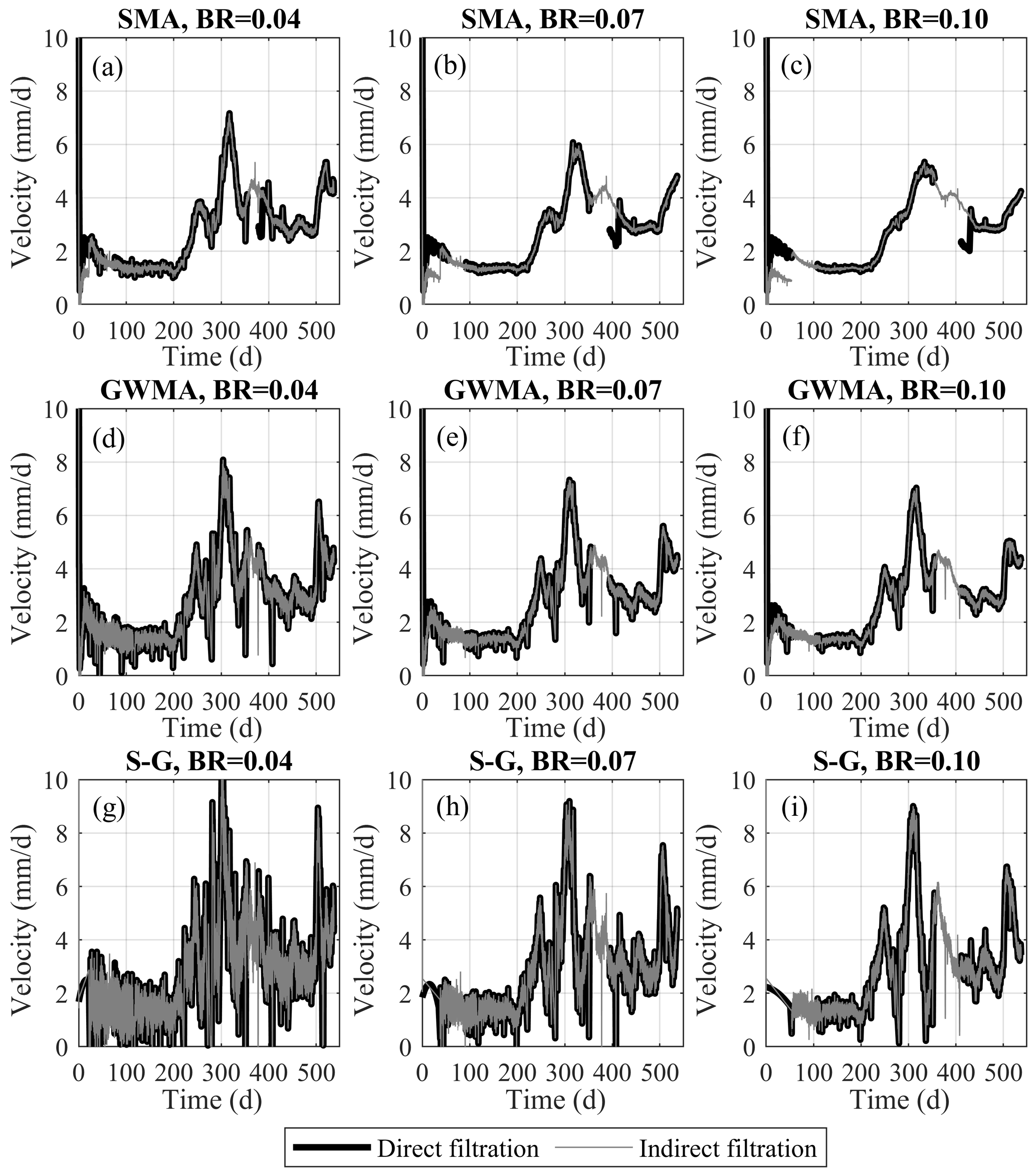
Figure 17Indirect and direct filtration results of Geocube no. 46 velocity values for bandwidth ratio (BR) values of (a) 0.04, (b) 0.07, and (c) 0.10.
Results for Geocube 47 confirm the same observations made for Geocube 46 but also allow for an evaluation of the significance of outliers on the filtered results. Figure 18a displays the outliers detected in the displacement diagram of Geocube 47 data along with the threshold established by the Hampel algorithm using an asymmetric window, a bandwidth of 0.4 %, and a threshold factor of 3. Figure 18b–d show a magnified portion of the displacement measurements for Geocube 47 filtered by each of the three filters at three different bandwidth ratios before the elimination of outliers. This highlights the necessity of outlier elimination before the application of any scatter filter. These plots show that detecting and removing outliers significantly impacts the performance of S-G as the presence of the outlier generates a peak that follows the outlier measurement and is followed by a sudden decrease that drops well beyond the data trend. SMA tends to widen the time range affected by the outlier more than GWMA, but, for the most part, the SMA-filtered results are almost parallel to the underlying trend. All filters appear to be significantly impacted by the outlier value, suggesting a pre-processing filter is required to remove outliers regardless of the use of SMA, GWMA, or S-G to reduce scatter. The outliers were successfully identified and removed after the application of the Hampel algorithm, and the above-mentioned effects were no longer observed in the filtered results.
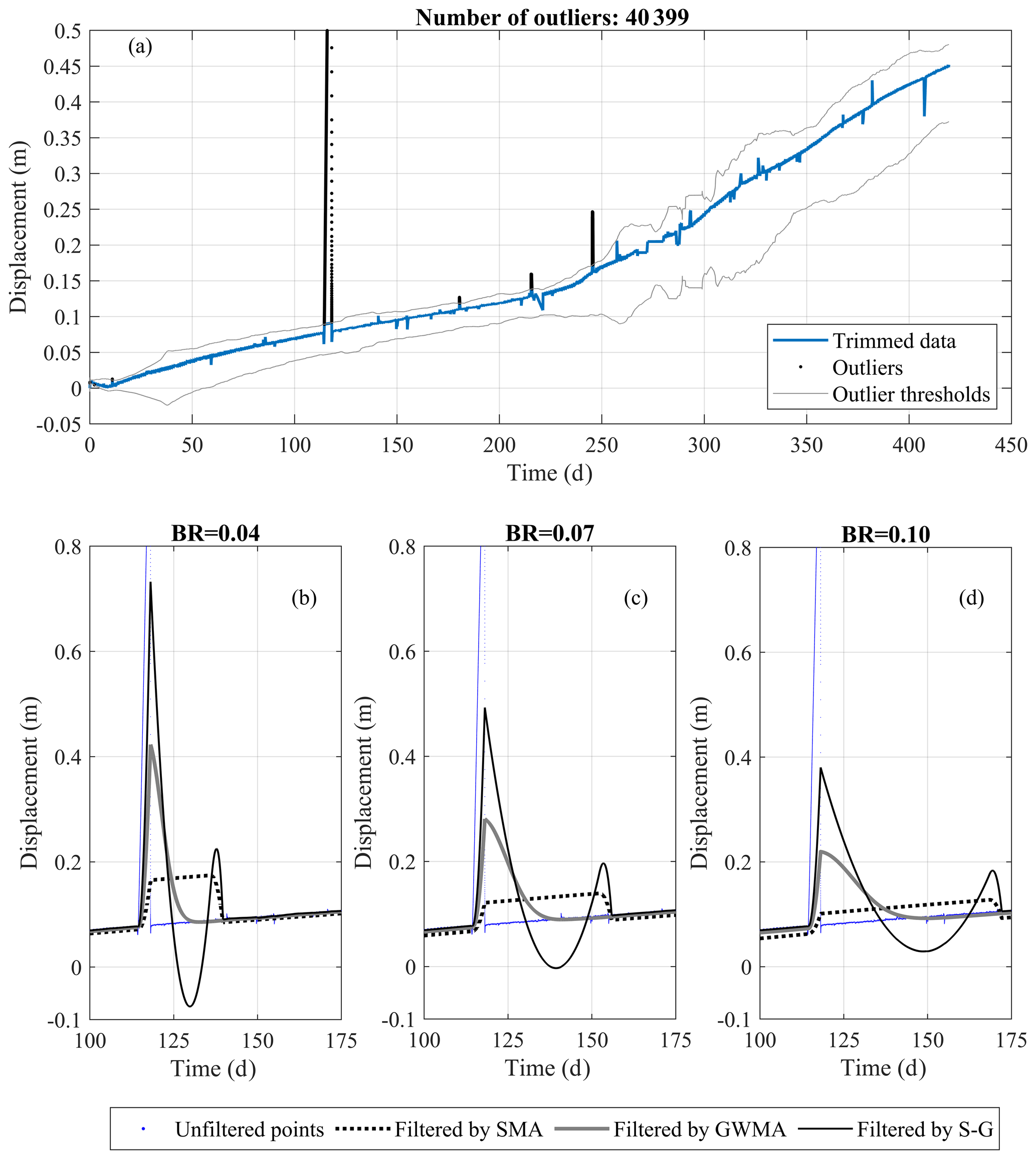
Figure 18Unfiltered and filtered displacement measurements for Geocube 47 at bandwidth ratios (BRs) of (a) 0.04, (b) 0.07, and (c) 0.10.
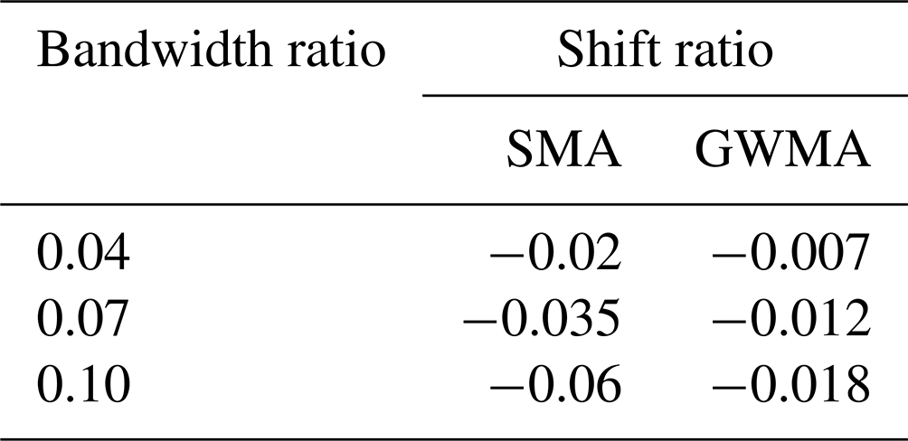
Table 3Shift ratios used for lag minimization of Geocube 46 displacements.
4.2.1 Lag minimization in filtered Geocube results
The lag between unfiltered and filtered data for Geocube 46 (Fig. 16) is consistent with the synthetic database results. The lag quantification results (Fig. 15b) were used to provide a correction value for the filtered Geocube results. The shift ratios used for this purpose with respect to each filter and bandwidth ratio are tabulated in Table 3. To determine whether the results of lag correction using the mean correlations derived from the synthetic scenarios (Table 2) were acceptable, the filtered diagrams were shifted (using the mean line for GWMA and values between the mean and lower boundary for SMA), and different portions of the displacement diagrams for Geocubes 46 and 47 were examined. Some examples are shown in Fig. 19. The mean and standard deviation of the scatter around the trend (error distribution) were calculated by assuming a linear trend within the short periods of analysis (considered an approximation of the true displacement trend for the short time interval). These were also calculated for the filtered and shifted diagrams. The closer the mean and standard deviation of the filtered and shifted data are to those obtained from the linear trend, the better the performance is of the lag correction based on the results from the synthetic scenarios. As an example, for the period from day 250 to 260, the GWMA resulted in a standard deviation of 0.001 to 0.0015 for bandwidth ratios from 0.04 to 0.10, respectively; corresponding values for SMA were 0.0018 to 0.0021. This illustrates that shifted GWMA results are closer to the true (scatter-free) displacements because the standard deviations of scatter inferred by this filter are closer to the true scatter, although both have good agreement with the true scatter. The means of inferred scatter by both filters are also close enough to the mean of the true scatter (almost zero). The results show the statistical indices of scatter inferred from the filtered shifted displacement measurements closely agree with that considered to be true scatter, and therefore the filtered displacement measurements are corrected for lag. This suggests the correlations stated in Fig. 15b and Table 2 based on the synthetic scenarios are applicable to minimize the lag for the Geocube system at the Ten-mile landslide.

Figure 19Mean and standard deviation of scatter inferred by SMA and GWMA in comparison with true scatter in the displacement of Geocube 46.
Previous studies dedicated to landslide monitoring consistently adopt SMA for scatter minimization in displacement data. However, the adequacy of this filter and the effect of bandwidth selection were not well understood. Analyses conducted on synthetic databases in this study using a roughness factor (J2) demonstrate that at least 4 % of the total observations should be fed into the filter to ensure fluctuations are sufficiently reduced.
The results of this study show that SMA tends to considerably distort the underlying trend at a bandwidth ratio of 0.10 (Figs. 8 and 9), and its lagged response with respect to real-time monitoring is almost 3 times that of GWMA results. As a result, a bandwidth ratio between 0.04 and 0.07 is suggested. However, we caution that the bandwidth should be selected with complete awareness that SMA is highly sensitive to bandwidth, and sensitivity analyses on bandwidth are recommended when defining an EWS. Corresponding observations were made during the analysis of displacement data from Geocubes installed on the Ten-mile landslide.
Error calculations show that GWMA and S-G outperform SMA in both direct and indirect filtration and are more successful in preserving the true displacement trend. The near-zero lagged response of S-G makes it a notable candidate for developing an EWS. Nonetheless, its intrinsic shortcoming in handling peaks, leading to a pulsating effect, will pose challenges for its utilization. The bandwidth range used for SMA is also suggested to be applied with the S-G filter.
GWMA results suggest a proper trade-off can be achieved between minimizing the lag time and scatter and avoiding the pulsating effect. Compared to SMA and S-G, GWMA is less sensitive to changes in the bandwidth. Analyses focused on the Geocube data also confirm that GWMA is capable of constraining the fluctuations in the velocity diagram while not attenuating variations in the displacement rate diagram. Moreover, the lag quantification chart proposed could reliably capture the required shift with a greater degree of confidence in comparison to SMA even at the largest bandwidth ratio studied here (0.10). The bandwidth for GWMA can therefore range from 0.04 to 0.10. Moreover, we observed consistency between direct and indirect filtration results using GWMA but greater differences when using SMA or S-G results. This was especially the case in the early parts of the datasets and at some locations where outlier elimination was likely ineffective.
Filter and bandwidth selections should not be arbitrarily or purely empirical, as differences in outcomes can be substantial. An automated surveillance system for landslides demands stability in filter performance for a variety of circumstances, considering the ground can experience irregular sequences of acceleration and deceleration. The results here suggest practice moves away from the adoption of SMA due to the limitations discussed. S-G demonstrates some inconsistent or erratic performance for certain displacement trends, which is detrimental, although overall the error is smaller than for SMA. On the balance of its strengths and limitations as evaluated in this study, GWMA appears to be the more robust approach.
This study evaluated the suitability of SMA, GWMA, and S-G filters for scatter reduction of datasets targeted for use in an EWS. A total of 12 different scenarios with harmonic and instantaneous changes were synthetically generated, and random variations with Gaussian distribution were then added to produce unfiltered results. The three filters considered were then each applied with different bandwidths, and the error was computed. These filters were also successfully applied to the records from two Geocubes installed on the Ten-mile landslide. The results led to the following conclusions:
-
When used for direct filtration of harmonic scenarios, the error resulting from the GWMA approach is approximately one-third that of the SMA approach. The S-G approach results in near-zero error regardless of the values of the bandwidth ratio and . When used for direct filtration of instantaneous scenarios, the superiority of S-G is no longer unconditional and depends on the bandwidth ratio; this reflects the fact that S-G cannot appropriately handle peaks in the velocity diagram.
-
When used for indirect filtration of harmonic scenarios, S-G again outperforms the other methods. The error associated with GWMA is marginally less than for SMA. These observations are not valid when the filters are applied to instantaneous scenarios as GWMA results in less error than S-G at bandwidth ratios above 0.03.
-
Detailed investigations with scenarios 11 and 12 demonstrate that SMA distorts the underlying trend by displacing and sometimes neglecting peak(s), while GWMA and S-G tend to preserve them somewhat similarly.
-
Due to the presence of negative weights in the S-G kernel, some artificial smaller troughs and peaks are created after major peaks. This phenomenon, referred to herein as a pulsating effect, results in an unfavourable performance of S-G on the velocity and displacement diagrams, especially in the presence of outliers.
-
Investigations on the roughness factor reveal the bandwidth ratio should be at least 0.04. Taking this into account, GWMA seems to be the most reasonable option as the related uncertainties are much smaller than for S-G and the error is acceptable and less than for SMA.
-
A consequence of using asymmetric windows in the filtering process is a lag in the SMA and GWMA results that increases with increasing bandwidth ratio. Lag quantification suggests a correlation between the needed shift and bandwidth ratio that can be used to eliminate the lag. SMA requires approximately 3 times the shift of GWMA on average.
-
Application of these filters to displacement data reported by Geocubes shows SMA and S-G are unable to properly handle data points at the beginning of the dataset (i.e., near the boundary) in indirect filtration of the velocity diagram. Moreover, SMA and S-G are inclined to, respectively, underestimate and overestimate peaks and fluctuations in the velocity diagram. Overall, GWMA provides the most reliable filtered values for velocity with no distinct difference between direct and indirect filtration.
Consider a polynomial of degree k that is intended to be fitted over an odd number of points denoted as z. The weighting coefficients of the Savitzky–Golay filter can be extracted from the first row of matrix C (Eq. 7):
where T operator is the transpose of a matrix, and J is the Vandermonde matrix, with elements at the ith row and jth column ( and ) that can be achieved as follows:
where m is the local index of points (). As an example, the kernel of an S-G filter that fits a quadratic polynomial (k=2) over seven points (z=7) is attained here. In the first step, J is set up as follows:
Then, using Eq. (1), matrix C is computed as Eq. (10):
The second and third rows of C are the coefficients to find the filtered values' first and second derivations at the point of interest, respectively.
The synthetic database can be generated through the comprehensive steps provided here. The Geocube measurements of the Ten-mile landslide displacement are not publicly available.
SS completed the conceptualization, developed the methodology, performed the analysis, and prepared the draft of this paper. MH and RM were supervisors of this study. The reviewing, draft editing, and project administration were conducted by MH, RM, and TE.
The contact author has declared that neither they nor their co-authors have any competing interests.
Publisher's note: Copernicus Publications remains neutral with regard to jurisdictional claims in published maps and institutional affiliations.
The authors thank Canadian National Railway (CN) for providing access to the Ten-mile site and for purchasing the Geocube units. This research was conducted through the (Canadian) Railway Ground Hazard Research Program, which is funded by the Natural Sciences and Engineering Research Council of Canada (NSERC ALLRP 549684-19), Canadian Pacific Railway, CN, and Transport Canada.
This research has been supported by the Natural Sciences and Engineering Research Council of Canada (grant no. NSERC ALLRP 549684-19).
This paper was edited by Filippo Catani and reviewed by Ugur Ozturk and one anonymous referee.
Atzeni, C., Barla, M., Pieraccini, M., and Antolini, F.: Early warning monitoring of natural and engineered slopes with ground-based synthetic-aperture radar, Rock Mech. Rock Eng., 48, 235–246, https://doi.org/10.1007/s00603-014-0554-4, 2015.
Benoit, L., Briole, P., Martin, O., and Thom, C.: Real-time deformation monitoring by a wireless network of a low-cost GPS, J. Appl. Geodesy, 8, 119–128, 2014.
Benoit, L., Briole, P., Martin, O., Thom, C., Malet, J. P., and Ulrich, P.: Monitoring landslide displacements with the Geocube wireless network of low-cost GPS, Eng. Geol., 195, 111–121, 2015.
BGC Engineering Inc.: CN Lillooet Sub. M. 167.7 (Fountain Slide) September 2015 Drilling and Instrumentation, Project report to Canadian National Railway, 2015.
BGC Engineering Inc.: CN Lillooet Sub. M. 167.7 (Ten Mile Slide) April 2016 Drilling and Instrumentation, Project report to Canadian National Railway, 2016.
Bovis, M. J.: Earthflows in the interior plateau, southwest British Columbia, Can. Geotech. J., 22, 313–334, 1985.
Bozzano, F., Mazzanti, P., and Moretto, S.: Discussion to: 'Guidelines on the use of inverse velocity method as a tool for setting alarm thresholds and forecasting landslides and structure collapses' by T. Carlà, E. Intrieri, F. Di Traglia, T. Nolesini, G. Gigli, and N. Casagli, Landslides, 15, 1437–1441, 2018.
Carlà, T., Farina, P., Intrieri, E., Botsialas, K., and Casagli, N.: On the monitoring and early-warning of brittle slope failures in hard rock masses: Examples from an open-pit mine, Eng. Geol., 228, 71–81, 2017a.
Carlà, T., Intrieri, E., Di Traglia, F., Nolesini, T., Gigli, G., and Casagli, N.: Guidelines on the use of inverse velocity method as a tool for setting alarm thresholds and forecasting landslides and structure collapses, Landslides, 14, 517–534, 2017b.
Carlà, T., Macciotta, R., Hendry, M., Martin, D., Edwards, T., Evans, T., Farina, P., Intrieri, E., and Casagli, N.: Displacement of a landslide retaining wall and application of an enhanced failure forecasting approach, Landslides, 15, 489–505, 2018.
Carlà, T., Intrieri, E., Raspini, F., Bardi, F., Farina, P., Ferretti, A., Colombo, D., Novali, F., and Casagli, N.: Perspectives on the prediction of catastrophic slope failures from satellite InSAR, Sci. Rep.-UK, 9, 1–9, 2019.
Carri, A., Valletta, A., Cavalca, E., Savi, R. and Segalini, A.: Advantages of IoT-based geotechnical monitoring systems integrating automatic procedures for data acquisition and elaboration, Sensors, 21, 2249, https://doi.org/10.3390/s21062249, 2021.
Casagli, N., Frodella, W., Morelli, S., Tofani, V., Ciampalini, A., Intrieri, E., Raspini, F., Rossi, G., Tanteri, L., and Lu, P.: Spaceborne, UAV and ground-based remote sensing techniques for landslide mapping, monitoring and early warning, Geoenviron. Disasters, 4, 1–23, 2017.
Chae, B. G., Park, H. J., Catani, F., Simoni, A., and Berti, M.: Landslide prediction, monitoring and early warning: a concise review of state-of-the-art, Geosci. J., 21, 1033–1070, 2017.
Chen, M. and Jiang, Q.: An early warning system integrating time-of-failure analysis and alert procedure for slope failures, Eng. Geol., 272, 105629, https://doi.org/10.1016/j.enggeo.2020.105629, 2020.
Clague, J. J. and Bobrowsky, P. T.: International year of planet earth 8. Natural hazards in Canada, Geosci. Can., 37, 17–37, 2010.
Cleveland, W. S.: LOWESS: A program for smoothing scatterplots by robust locally weighted regression, Am. Stat., 35, 54, https://doi.org/10.2307/2683591, 1981.
Cleveland, W. S. and Devlin, S. J.: Locally weighted regression: an approach analysis by local fitting, J. Am. Stat. Assoc., 83, 596–610, 1988.
Clifford, P.: Monte Carlo methods, in: Statistical methods for Physical Science, edited by: Stanford, J. L. and Vardeman, S. B., Elsevier, San Diego, California, 125–153, 1994.
Davies, L. and Gather, U.: The identification of multiple outliers, J. Am. Stat. Assoc., 88, 782–792, 1993.
Deane, E.: The Application of Emerging Monitoring Technologies on Very Slow Vegetated Landslides, Dissertation, University of Alberta, Edmonton, Alberta, Canada, 2020.
Desrues, M., Malet, J. P., Brenguier, O., Carrier, A., Mathy, A., and Lorier, L.: Landslide kinematics inferred from in situ measurements: the Cliets rock-slide (Savoie, French Alps), Landslides, 19, 19–34, https://doi.org/10.1007/s10346-021-01726-1, 2022.
Dick, G. J., Eberhardt, E., Cabrejo-Liévano, A. G., Stead, D. and Rose, N. D.: Development of an early-warning time-of-failure analysis methodology for open-pit mine slopes utilizing ground-based slope stability radar monitoring data, Can. Geotech. J., 52, 515–529, 2015.
Donati, D., Stead, D., Lato, M., and Gaib, S.: Spatio-temporal characterization of slope damage: insights from the Ten Mile Slide, British Columbia, Canada, Landslides, 17, 1037–1049, 2020.
Dorberstein, D.: Fundamentals of GPS Receivers: A Hardware Approach, Springer Science & Business Media, Nipomo, CA, USA, 2011.
Gaib, S., Wilson, B., and Lapointe, E.: Design, construction and monitoring of a test section for the stabilization of an active slide area utilizing soil mixed shear keys installed using cutter soil mixing, in: Proceedings of the ISSMGE – TC 211 International Symposium on Ground Improvement IS-GI, Brussels, 31 May–1 June, 3, 147–158, 2012.
Grebby, S., Sowter, A., Gluyas, J., Toll, D., Gee, D., Athab, A., and Girindran, R.: Advanced analysis of satellite data reveals ground deformation precursors to the Brumadinho Tailings Dam collapse, Communications Earth & Environment, 2, 1–9, 2021.
Guthrie, R. H.: Socio-Economic Significance: Canadian Technical Guidelines and Best Practices Related to Landslides: A National Initiative for Loss Reduction, Natural Resources Canada, Ottawa, ON, 2013.
Hampel, F. R.: A general qualitative definition of robustness, Ann. Math. Stat., 42, 1887–1896, 1971.
Hongtao, N.: Smart safety early warning model of landslide geological hazard based on BP neural network, Safety Sci., 123, 104572, https://doi.org/10.1016/j.ssci.2019.104572, 2020.
Huntley, D., Bobrowsky, P., Charbonneau, F., Journault, J., Macciotta, R., and Hendry, M.: Innovative landslide change detection monitoring: application of space-borne InSAR techniques in the Thompson River valley, British Columbia, Canada, Workshop on World Landslide Forum, Ljubljana, Slovenia, 11–13 October, 3, 219–229, 2017.
Intrieri, E., Gigli, G., Mugnai, F., Fanti, R., and Casagli, N.: Design and implementation of a landslide early warning system, Eng. Geol., 147, 124–136, 2012.
Intrieri, E., Raspini, F., Fumagalli, A., Lu, P., Del Conte, S., Farina, P., Allievi, J., Ferretti, A., and Casagli, N.: The Maoxian landslide as seen from space: detecting precursors of failure with Sentinel-1 data, Landslides, 15, 123–133, 2018.
Journault, J., Macciotta, R., Hendry, M. T., Charbonneau, F., Huntley, D., and Bobrowsky, P. T.: Measuring displacements of the Thompson River valley landslides, south of Ashcroft, BC, Canada, using satellite InSAR, Landslides, 15, 621–636, 2018.
Karl, J. H.: Introduction to Digital Signal Processing, Academic Press, San Diego, 1989.
Kothari, U. C. and Momayez, M.: New approaches to monitoring, analyzing and predicting slope instabilities, Journal of Geology and Mining Research, 10, 1–14, 2018.
Lacasse, S. and Nadim, F.: Landslide risk assessment and mitigation strategy, in: Landslides–Disaster Risk Reduction, edited by: Sassa, K. and Canuti, P., Springer, Berlin, Heidelberg, 31–61, 2009.
Leroueil, S.: Natural slopes and cuts: movement and failure mechanisms, Géotechnique, 51, 197–243, 2001.
Liu, H., Shah, S., and Jiang, W.: On-line outlier detection and data cleaning, Comput. Chem. Eng., 28, 1635–1647, 2004.
Macciotta, R. and Hendry, M. T.: Remote sensing applications for landslide monitoring and investigation in western Canada, Remote Sens.-Basel, 13, 366–389, 2021.
Macciotta, R., Hendry, M., and Martin, C. D.: Developing an early warning system for a very slow landslide based on displacement monitoring, Nat. Hazards, 81, 887–907, 2016.
Macciotta, R., Carlà, T., Hendry, M., Evans, T., Edwards, T., Farina, P., and Casagli, N.: The 10-mile Slide and response of a retaining wall to its continuous deformation, Workshop on World Landslide Forum, Ljubljana, Slovenia, 11–13 October, 553–562, 2017a.
Macciotta, R., Rodriguez, J., Hendry, M., Martin, C. D., Edwards, T., and Evans, T.: The 10-mile Slide north of Lillooet, British Columbia–history, characteristics, and monitoring, in: Proceedings, 3rd North American Symposium on Landslides, Roanoke, Virginia, 4–8 June, 937–948, 2017b.
Pearson, R. K.: Outliers in process modeling and identification, IEEE Trans. Contr. Syst. T., 10, 55–63, 2002.
Reid, M. E., Godt, J. W., LaHusen, R. G., Slaughter, S. L., Badger, T. C., Collins, B. D., Schulz, W. H., Baum, R. L., Coe, J. A., Harp, E. L. and Schmidt, K. M.: When hazard avoidance is not an option: lessons learned from monitoring the postdisaster Oso landslide, USA, Landslides, 18, 2993–3009, 2021.
Rodriguez, J. L., Macciotta, R., Hendry, M., Edwards, T., and Evans, T.: Slope hazards and risk engineering in the Canadian railway network through the Cordillera, in: Proceedings of the AIIT International Congress on Transport Infrastructure and Systems (TIS 2017), Rome, Italy, 10–12 April, 163–168, 2017.
Rodriguez, J., Hendry, M., Macciotta, R., and Evans, T.: Cost-effective landslide monitoring GPS system: characteristics, implementation, and results, Geohazards7, Canmore, Alberta, 3–6 June, 2018.
Rodriguez, J., Macciotta, R., Hendry, M. T., Roustaei, M., Gräpel, C., and Skirrow, R.: UAVs for monitoring, investigation, and mitigation design of a rock slope with multiple failure mechanisms – a case study, Landslides, 17, 2027–2040, 2020.
Rousseeuw, P. J. and Hubert, M.: Robust statistics for outlier detection, WIREs Data Min. Knowl., 1, 73–79, 2011.
Salgado, C. M., Azevodo, C., Proença, H., and Vieira, S. M.: Noise versus outliers, in: Secondary Analysis of Electronic Health Records, by: MIT Critical Data, Springer, Cambridge, Massachusetts, 163–183, 2016.
Savitzky, A. and Golay, M. J.: Smoothing and differentiation of data by simplified least squares procedures, Anal. Chem., 36, 1627–1639, 1964.
Schafer, M. B.: Kinematics and Controlling Mechanics of Slow-moving Ripley Landslide, Dissertation, University of Alberta, Edmonton, Alberta, Canada, 2016.
Schafer, R. W.: What is a Savitzky–Golay filter? [lecture notes], IEEE Signal Proc. Mag., 28, 111–117, 2011.
Scoppettuolo, M. R., Cascini, L., and Babilio, E.: Typical displacement behaviours of slope movements, Landslides, 17, 1105–1116. 2020.
Smith, S.: Digital Signal Processing: A Practical Guide for Engineers and Scientists, Elsevier, Burlington, Massachusetts, 2013.
Thiebes, B., Bell, R., Glade, T., Jäger, S., Mayer, J., Anderson, M., and Holcombe, L.: Integration of a limit-equilibrium model into a landslide early warning system, Landslides, 11, 859–875, 2014.
Tofani, V., Rasipini, F., Catani, F., and Casagli, N.: Persistent Scatterer Interferometry (PSI) technique for landslide characterization and monitoring, Remote Sens.-Basel, 5, 1045–1065, 2013.
UNISDR: United Nations International Strategy for Disaster Reduction: Terminology on Disaster Risk Reduction, International Strategy for Disaster Reduction, Geneva, Switzerland, available at: http://www.unisdr.org (last access: 12 February 2021), 2009.
Vaziri, A., Moore, L., and Ali, H.: Monitoring systems for warning impending failures in slopes and open pit mines, Nat. Hazards, 55, 501–512, 2010.
Wang, G.: GPS landslide monitoring: single base vs. network solutions-a case study based on the Puerto Rico and Virgin Islands permanent GPS network, J. Geodet. Sci., 1, 191–203, 2011.
William, S. C.: Robust locally weighted regression and smoothing scatterplots, J. Am. Stat. Assoc., 74, 829–836, 1979.
Woods, A., Hendry, M. T., Macciotta, R., Stewart, T., and Marsh, J.: GB-InSAR monitoring of vegetated and snow-covered slopes in remote mountainous environments, Landslides, 17, 1713–1726, 2020.
Woods, A., Macciotta, R., Hendry, M. T., Stewart, T., and Marsh, J.: Updated understanding of the deformation characteristics of the Checkerboard Creek rock slope through GB-InSAR monitoring, Eng. Geol., 281, 105974, https://doi.org/10.1016/j.enggeo.2020.105974, 2021.
Yao, Z., Xie, J., Tian, Y., and Huang, Q.: Using Hampel identifier to eliminate profile-isolated outliers in laser vision measurement, J. Sensors, 2019, 3823691, https://doi.org/10.1155/2019/3823691, 2019.
Yin, Y., Wang, H., Gao, Y., and Li, X.: Real-time monitoring and early warning of landslides at relocated Wushan Tow, the Three Gorges Reservoir, China, Landslides, 7, 339–349, 2010.
Zhang, Y. G., Tang, J., He, Z. Y., Tan, J., and Li, C.: A novel displacement prediction method using gated recurrent unit model with time series analysis in the Erdaohe landslide, Nat. Hazards, 105, 783–813, 2021.
Zhang, Y. H., Ma, H. T. and Yu, Z. X.: Application of the method for prediction of the failure location and time based on monitoring of a slope using synthetic aperture radar, Environ. Earth Sci., 80, 1–13, 2021.
Zhou, X. P., Liu, L. J., and Xu, C.: A modified inverse-velocity method for predicting the failure time of landslides, Eng. Geol., 268, 105521, https://doi.org/10.1016/j.enggeo.2020.105521, 2020.
Zimek, A. and Filzmoser, P.: There and back again: Outlier detection between statistical reasoning and data mining algorithms, WIREs Data Min. Knowl., 8, 1280, https://doi.org/10.1002/widm.1280, 2018.