the Creative Commons Attribution 4.0 License.
the Creative Commons Attribution 4.0 License.
 | 01 Nov 2022
Building-scale flood loss estimation through vulnerability pattern characterization: application to an urban flood in Milan, Italy
Andrea Taramelli
Margherita Righini
Emiliana Valentini
Lorenzo Alfieri
Ignacio Gatti
Simone Gabellani
The vulnerability of flood-prone areas is determined by the susceptibility of the exposed assets to the hazard. It is a crucial component in risk assessment studies, both for climate change adaptation and disaster risk reduction. In this study, we analyse patterns of vulnerability for the residential sector in a frequently hit urban area of Milan, Italy. The conceptual foundation for a quantitative assessment of the structural dimensions of vulnerability is based on the modified source–pathway–receptor–consequence model. This conceptual model is used to improve the parameterization of the flood risk analysis, describing (i) hazard scenario definitions performed by hydraulic modelling based on past event data (source estimation) and morphological features and land-use evaluation (pathway estimation) and (ii) the exposure and vulnerability assessment which consists of recognizing elements potentially at risk (receptor estimation) and event losses (consequence estimation). We characterized flood hazard intensity on the basis of variability in water depth during a recent event and spatial exposure also as a function of a building's surroundings and buildings' intrinsic characteristics as a determinant vulnerability indicator of the elements at risk. In this sense the use of a geographic scale sufficient to depict spatial differences in vulnerability allowed us to identify structural vulnerability patterns to inform depth–damage curves and calculate potential losses from mesoscale (land-use level) to microscale (building level). Results produces accurate estimates of the flood characteristics, with mean error in flood depth estimation in the range 0.2–0.3 m and provide a basis to obtain site-specific damage curves and damage mapping. Findings show that the nature of flood pathways varies spatially, is influenced by landscape characteristics and alters vulnerability spatial distribution and hazard propagation. At the mesoscale, the “continuous urban fabric” Urban Atlas 2018 land-use class with the occurrence of at least 80 % of soil sealing shows higher absolute damage values. At microscale, evidence demonstrated that even events with moderate magnitude in terms of flood depth in a complex urbanized area may cause more damage than one would expect.
- Article
(20959 KB) - Full-text XML
- BibTeX
- EndNote


Flood risk is not stationary; it hinges on climate variability along with changes in vulnerability patterns of exposed elements (Lal et al., 2012). Climate change and socio-economic developments strongly affect such natural dynamics, which include changes in the probability or intensity of hazards (Elmer et al., 2010; Cammerer et al., 2013; Cammerer and Thieken, 2013) associated with human-induced environmental changes. Vulnerability of elements at risk and the communities' adaptive capacity variations rely on socio-economic developments entailing land use and changes in the exposure of people and assets (Hufschmidt et al., 2005; Bouwer et al., 2010; Meyer et al., 2013; Taramelli et al., 2018). Hence, within flood-prone areas one of the cost-effective ways to manage and adapt to floods is through a flood vulnerability assessment. Vulnerability can be described as (1) multi-dimensional (e.g. physical, social-cultural, socio-economic and environmental) (Balica et al., 2009); (2) dynamic (i.e. vulnerability changes over time); (3) scale-dependent (i.e. vulnerability can be assessed at various spatial and temporal scales) (Fekete et al., 2010; Lal et al., 2012); and (4) site-specific (i.e. the approach is defined by a specific location's needs) (Vogel and O'Brien, 2004). Thus, it is essential to address the drivers of vulnerability, how it increases, and how it is distributed to effectively manage risk. Therefore, understanding, quantifying and analysing the vulnerability and exposure of physical properties are prerequisites for designing strategies and adopting an approach for its reduction (Papathoma-Köhle et al., 2019). We focus here on the structural dimension of vulnerability of flood-prone areas that has proven to be key in analysing flood risk. Since the structural vulnerability is defined as the potential of a particular class of buildings or infrastructure facilities to be affected or damaged under a given flood intensity (Faella and Nigro, 2003), damage by flood hazard depends on the vulnerability of exposed buildings (Schanze, 2006; Merz et al., 2010). Vulnerability matrices, depth–damage curves and vulnerability indices (Balica et al., 2009; Papathoma-Köhle et al., 2019) or indicator-based methodology (Kappes et al., 2012) are methods and approaches mainly used for physical vulnerability assessment (Fuchs et al., 2019; Kumar and Bhattacharjya, 2020; Malgwi et al., 2020). The indicator-based methods usually provide a scale of flood vulnerability to elements at risk, having the strength of allowing significant factors that contribute to flood vulnerability to be understood easily by potential users. However, though the indicator-based method does not require a significant amount of field flood damage records and empirical studies unlike the quantitative method usually expressed by the depth–damage curve functions, they are not for monetary flood vulnerability assessment (Usman Kaoje et al., 2021). Conversely, depth–damage functions estimate direct and tangible quantifiable damage normally defined by interpolating flooding depth and damage data of a specific asset, economic sector or land-use category (Nasiri et al., 2016), estimating the potential effects of a given flood depth in the investigated area. There are several damage assessments models which have been based on different approaches and amount of variables. Empirical approaches are developed based on damage data compiled after flood events, while synthetic damage models are expert-based models obtained by a what-if analysis (Thieken et al., 2008; Roberts et al., 2009; Pistrika et al., 2014; Amadio et al., 2019; Arrighi et al., 2020). On one side empirical curves give more accurate actual damage data, and on the other synthetic functions show more transferability and comparability. However, their reliability strongly depends on the quality and quantity of input data used (Molinari and Scorzini, 2017; Englhardt et al., 2019). The problem is further exacerbated by the lack of information on damage explicatory variables, both hazard and vulnerability related (Molinari et al., 2012; Menoni et al., 2016). Akbas et al. (2009) proposed a specific physical vulnerability curve introducing the concept of probabilistic damage functions and appropriate definitions of relevant damage states, assessing temporal and spatial impact probability uncertainties. As a result of neglected attention to disaster risk impacts in the past, it is not easy or even possible to portray the spatial and temporal patterns of flood damage and losses with reasonable precision. This makes measurement of progress in reducing the disaster risk difficult if not infeasible. Therefore, some authors stressed the need for the use of empirical data from past events to provide powerful analytical tools (Apel et al., 2008; Vamvatsikos et al., 2010; Kreibich et al., 2022). The ideal solution would be a model that is simple, as the empirical ones, but that includes quantitative and qualitative explicative parameters in damage assessment, as the synthetic ones, to capture the full complexity of buildings vulnerability (Schanze, 2006; Balica et al., 2009; Lal et al., 2012; Morelli et al., 2021). The aim of this paper is to improve structural vulnerability assessment for a flood prone area considering vulnerability to be a composition of the hazard intensity and inherent characteristics of elements at risk and their surroundings as sources of information to define the more susceptible and exposed residential buildings to inform depth–damage curves and calculate potential losses and damage maps. To better understand potentially damaging natural processes interacting with elements at risk, the work is structured according to the modified source–pathway–receptor–consequence (SPRC) conceptual model (Fleming, 2002). The SPRC model relies on a simple causal chain commonly adopted to understand the flood risk system and the link among processes (Schanze, 2006). The SPRC model consists of the hazard origin identification as an event transmitted through a pathway to a receptor with possible negative effects for the receptor depending on their vulnerability and their exposure intensity (Hallegatte et al., 2013; Taramelli et al., 2015). The SPRC model considers the hazards as the flood water that propagates to the receptor resulting in potential consequences (Hallegatte et al., 2013; Taramelli et al., 2015).
-
The “source” of a flood is the origin of the hazard, usually an extreme meteorological event (e.g. heavy rainfall) triggering floods.
-
The “pathway” is the route that a hazard takes to get to the receptors. A pathway must exist for a hazard to be realized.
-
The “receptor” refers to the entities that may be damaged by the hazard depending on their exposure and susceptibility (e.g. people, property or the environment).
-
The “consequence” is the harm that results from a single occurrence of the hazard, such as economic, social or environmental that may result from a flood. It may be expressed quantitatively (e.g. monetary value), by category (e.g. high, medium, low) or descriptively (USACE, 2019).
Here vulnerability assesses the susceptibility to harm of exposed residential buildings when exposed to the hazard (USACE, 2019; Kreibich et al., 2022) to (1) address the necessity of an integrated qualitative and quantitative approach to define flood physical (structural) vulnerability; (2) to accurately re-assess past event flood characteristics; (3) to bridge the gap of vulnerability spatialization using spatially distributed information to obtain vulnerability mapping and related potential damage suitable for giving indications on where and how to reduce risks at local level; (4) to bridge the lack of reliable input data in particular regarding the properties of the elements at risk (i.e. the exposure and susceptibility factors) that also contribute to their vulnerability at building level; and (5) to improve the exposure analysis integrating the building's surroundings as a vulnerability indicator (i.e. morphological features and land use). The article is organized as follows: after introducing the current methods to assess flood vulnerability and applications, Sect. 2 describes the case study. Section 3 addresses in detail the input data used and the analytic four steps of the SPRC approach to accurately assess the structural vulnerability. Section 4 depicts the structural vulnerability patterns characterized and classified in terms of their hazard to fluvial flooding based on data from the 2014 Seveso River flood event (source and pathway) and exposure, the developing of site-specific damage curves for the residential sector element at risk at meso- (i.e. land-use level) and microscale (i.e. building level), and the damage mapping (receptor and consequence). Section 5 discusses the results of the study, pointing out the advantages, limitations and future developments, and, finally, Sect. 6 summarizes the derived conclusions.
The Lombardy region, Italy's economic engine, is particularly vulnerable to flood risk (Carrera et al., 2015). It is indeed the most flood-affected region in terms of financial damage, consequently influencing the national growth and stability. The northern part of the city of Milan (45∘28′ N, 09∘11′ E) is frequently flooded by the floodwaters of the Seveso River. A total of 342 floods were reported in the last 140 years (i.e. 2.6 per year) (Becciu et al., 2018). On 14 July 2014 after a short and intense storm that dropped more than 60 mm of precipitation within 5 h, the Seveso River overflowed in a few sections along its course and flooded some densely populated areas in the provinces of Como, Monza–Brianza, and Milan. Notably, an area of about 3 km2 in the northern part of the city of Milan was flooded, causing closure of streets and public transport and affecting thousands of inhabitants (Davies, 2014). The Seveso River overflowed at two sections at Niguarda (via Ca' Granda), flowing out of manholes and generating fountains of water and mud that completely inundated Viale Zara and the whole neighbourhood, which is frequently hit by similar events. The flood caused serious damage to cars, shops, basements and ground floors of many residential buildings. The Isola neighbourhood, near the historic city centre, was also affected, and the area of Piazza Minniti was completely inundated. Throughout the northern part of the city, roads were paralysed for many hours. Official loss data provided by the Lombardy Region based on the damage report form in the frame of the loss compensation by the state, reported a total damage of EUR 27.2 million. Private owners were the most impacted (64 %), followed by infrastructure (18 %), commercial activities (13 %), the industrial sector (5 %) and the environmental (0.4 %) (Fig. 1).
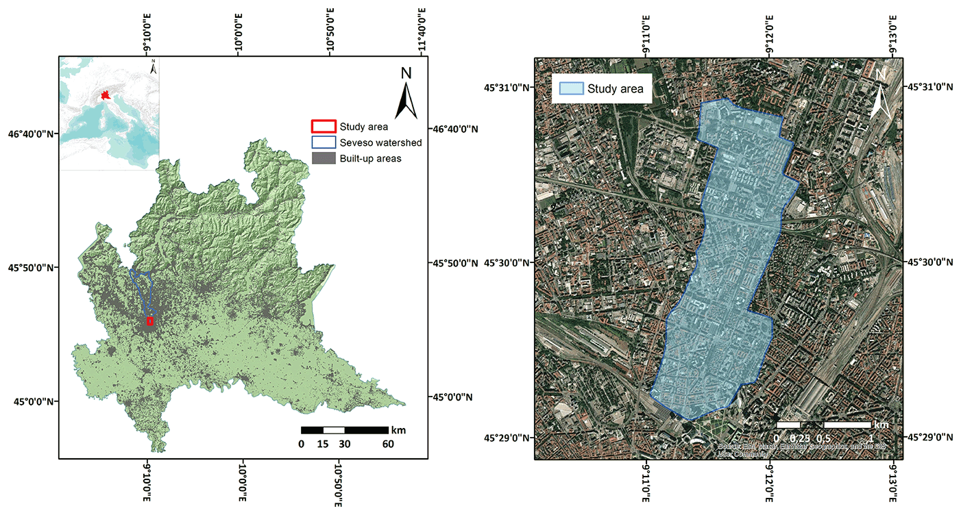
Figure 1Investigation area and survey of inundated area of the 2014 Seveso flood in Milan. Base map and DTM from © Regione Lombardia 2022. Built-up-area shapefile is from © OpenStreetMap contributors 2022. Distributed under the Open Data Commons Open Database License (ODbL) v1.0. Satellite image is from © Google Earth 2022.
In this section we address in detail the analytic four steps of the SPRC model (Fig. 2a) and the data used to accurately assess the structural vulnerability patterns and to understand the links among flood risk system processes (Fig. 2b).
-
Source estimation. We reassessed the “inundation map” replicating the flood characteristics providing the flood water depth extension for the study area's affected zones.
-
Pathway estimation. We defined inland attributes that can control and influence the event propagation to define in the following step the exposure.
-
Receptor estimation. We considered the elements at risk to perform the exposure and susceptibility analysis to finally assess structural vulnerability. Thus, elements that are exposed and susceptible to hazard have been categorized into vulnerability homogenous classes.
-
Consequence estimation. We developed site-specific damage curves for the residential sector at meso- (i.e. land-use level) and microscale (i.e. building level) considering the 2014 flood event and three diverse flood scenarios assuming return periods of 10, 100 and 500 years (Nafari, 2013).
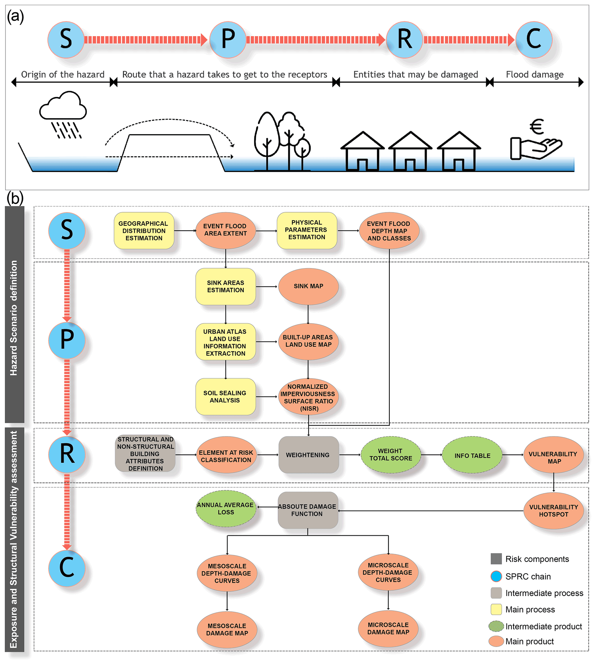
Figure 2(a) SPRC conceptual model. (b) Structural vulnerability assessment procedure overview using a modified SPRC model.
In the first three steps we identified significant and suitable vulnerability indicators in urban areas representative of three components that contribute to the vulnerability of the elements at risk, i.e. flood hazard intensity, effect of the surrounding environment and building characteristics, to produce a vulnerability map at building scale aggregating the indicators and their weights for the selected physical flood, whereas in the last step structural vulnerability patterns are used to inform depth–damage curves and calculate potential losses from mesoscale (land-use level) to microscale (building level).
3.1 Hazard scenario definitions: source and pathway estimation
3.1.1 Source estimation
Polygons of the flooded area for this event were collected through the geoportal of the Lombardy region. The main data source is represented by surveys and observations from the affected municipalities. A flood-related hazard map of the 2014 flood event is attained by reconstructing the flood-affected area and replicating the flood characteristics (i.e. depth of flood water) using the Floodwater Depth Estimation Tool version 2 (FwDET) (Cohen et al., 2019) implemented in Google Earth Engine. FwDET identifies the floodwater elevation for each cell within a flooded domain based on its nearest flood-boundary grid cell here derived from the digital terrain model (DTM) of the Lombardy Region with a spatial resolution of 5 by 5 m (Bocci et al., 2015).
3.1.2 Pathway estimation
Morphological features and land use were also considered important factors in influencing hazard propagation. We investigated endangered urban residential areas located within or near landscape sinks (SIs) that are potentially filled in conditions of flooding and inefficient drainage systems (Dietrich and Perron, 2006; Dodov and Foufoula-Georgiou, 2006; Nardi et al., 2006; Taramelli and Reichenbach, 2008; Thrysøe et al., 2021). These low-lying areas are defined including the DTM 5×5 m and the buildings' footprint layer into a sequential chain of GIS analysis tools. This model is based on the screening of a DTM for landscape depressions and their maximum extent when filled up at the capacity before spilling over during a flood while ignoring local infiltration rates and time, thereby allowing the model to select buildings inside or adjacent to these low-lying areas. As the analysis was focused on residential sector damage, exposure information related only to built-up areas was extracted from Copernicus Urban Atlas 2018 (European Union, Copernicus Land Monitoring Service, European Environment Agency, 2018a). These data are exploited to determine how flood vulnerability could rise as a combination of environmental and climate changes effects (Taramelli et al., 2019). Therefore, the Copernicus High Resolution Layer Imperviousness Density 2018 (European Union, Copernicus Land Monitoring Service, European Environment Agency, 2018b) with a resolution of 20 m resampled by nearest-neighbours at 5 m is used to identify the most exposed residential buildings. Specifically, the normalized imperviousness surface ratio (NISR) was introduced to obtain a proxy to identify buildings most exposed to hazard amplification due to soil sealing (S.L., as stated in the Land Cover/Land Use product nomenclature of the Copernicus Urban Atlas), Eq. (1).
3.2 Exposure and structural vulnerability assessment: receptor and consequence estimation
At the building level, relevant structural indicators (e.g. the building type, the period of construction, the material type, the maintenance state and building height) are important for determining the susceptibility due to flooding allowing specific building type classifications. The structural and non-structural building attributes were linked to the physical characteristics of the damaging flood events to
-
define building susceptibility and finally assess structural vulnerability applying a geographically distributed and weight-base procedure at building level, the heuristic approach (receptor estimation);
-
evaluate the buildings' potential damage by flood hazards, developing site-specific damage curves based at both land-use and building levels, the probabilistic approach (consequence estimation).
3.2.1 Receptors estimation: heuristic approach
By overlapping hazard and exposure maps (i.e. the spatial distribution of the elements at risk), a corresponding hazard class is assigned to each building (see Appendix A). This defines the magnitude of the damaging flood assigned to each element at risk. Furthermore, at a residential building level relevant descriptive structural attributes are important for determining the susceptibility due to flooding allowing specific building type classifications (Figueiredo and Martina, 2016). The structural type combined with the construction materials determine the strength of the building (Corradi et al., 2015). Age and maintenance are also indications for the current state of the building. Moreover, an estimation of element-at-risk costs is fundamental to express potential losses in economic terms. The heuristic approach is based on a simple equal-weight assignment procedure (Taramelli et al., 2015). The weight assignment has been given by the authors based on an intensive literature review and on data availability and quality. The indicators are identified as significant and suitable vulnerability indicators in urban areas representative of three components, i.e. flood hazard intensity, effect of the surrounding environment and building characteristics. A total score (Eq. 2) is calculated as the sum of single weights assigned to hazard and pathway (i.e. for water depth, WD, on the basis of the level (in m) of inland flooding raster maps, on sink SI map and on NISR classes) (Table 1) and to each structural and non-structural indicator (i.e. construction material type, MT, period of construction, PC, building status, BS, building height, BH, building type, BT) composing an element at risk. Weights are assigned from 1 = “no or very low response capacity” to 9 = “high response capacity” against flood (Table 2) (Corradi et al., 2015) and based on the literature review (Taramelli et al., 2015).
Hence, an info-table of residential buildings classified by total score is obtained. Residential buildings were classified in five vulnerability classes based on the obtained info-table from “very low” to “very high” vulnerability (Table 3) using the Jenks natural break algorithm. With the natural break classification (Jenks), classes are based on natural groupings inherent in the data maximizing the differences between classes. Hereafter buildings were mapped considering the economic unit value (in EUR m−2) based on the National Real Estate Observatory (OMI) zone and the relative market value quotation (EUR m−2) table obtained from OMI assigned to each residential building type (BT) on the basis of the building status (BS). Here the building economic unit value has been used for estimating the exposed assets in terms of monetary exposure of the residential buildings in the flooded area assuming solely the structure value and excluding the content value. For buildings falling in the most vulnerable classes (i.e. classes 1 and 2, “very high” and “high”), a distinction was made between elements with and without a basement (Arrighi et al., 2020; Molinari et al., 2020), assigning a weight of 0 to the building with a basement and 1 to the building without a basement based on the level of damage estimated by McBean et al. (1988) and Crigg and Helweg (1975). As previously mentioned, the assignment of weights refers to the building's response capacity against flood hazard, meaning the capability or incapability of an object to resist the flood impact. Hence, lower values correspond to lower response capacity (high-vulnerability buildings), whereas higher values correspond to higher response capacity (low-vulnerability buildings) (Taramelli et al., 2015).
Table 1Weights related to hazard classes for flood depth assigned to residential buildings, on sink map and on NISR classes.
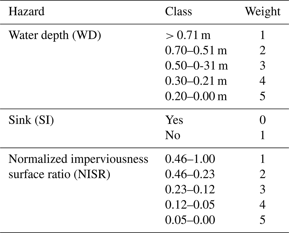
Table 2Weights assigned to each structural feature composing residential buildings, such as MT (i.e. construction material type), PC (i.e. period of construction), BS (i.e. building status), BH (i.e. building height) and BT (i.e. building type).
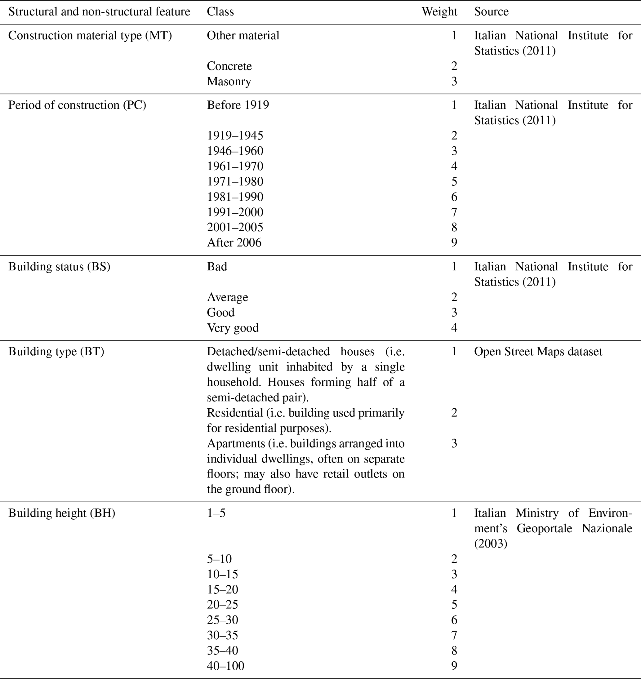
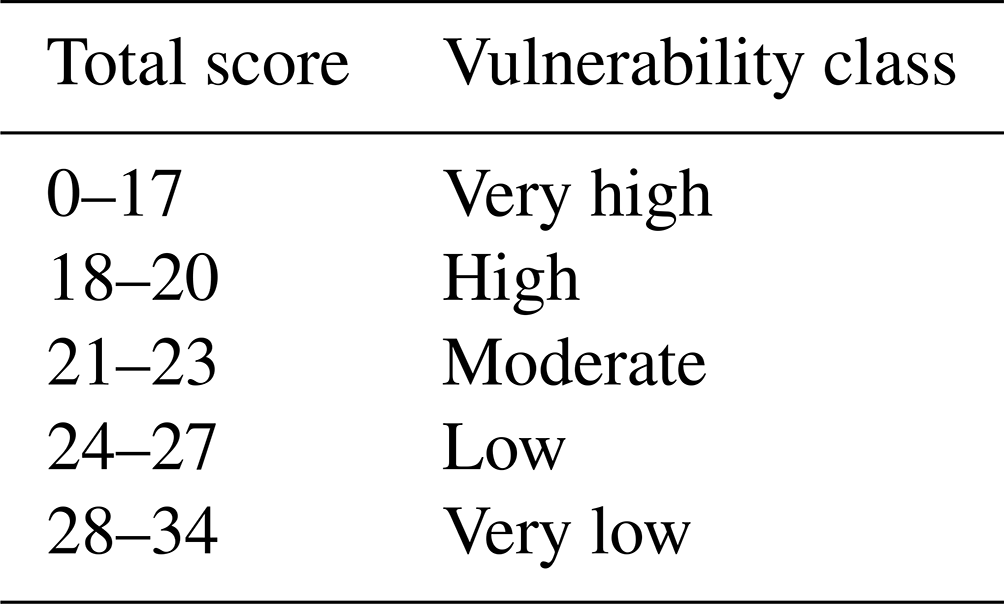
Table 3Total score and vulnerability classes (“very high”, “high”, “moderate”, “low”, “very low”).
3.2.2 Consequence estimation: probabilistic approach
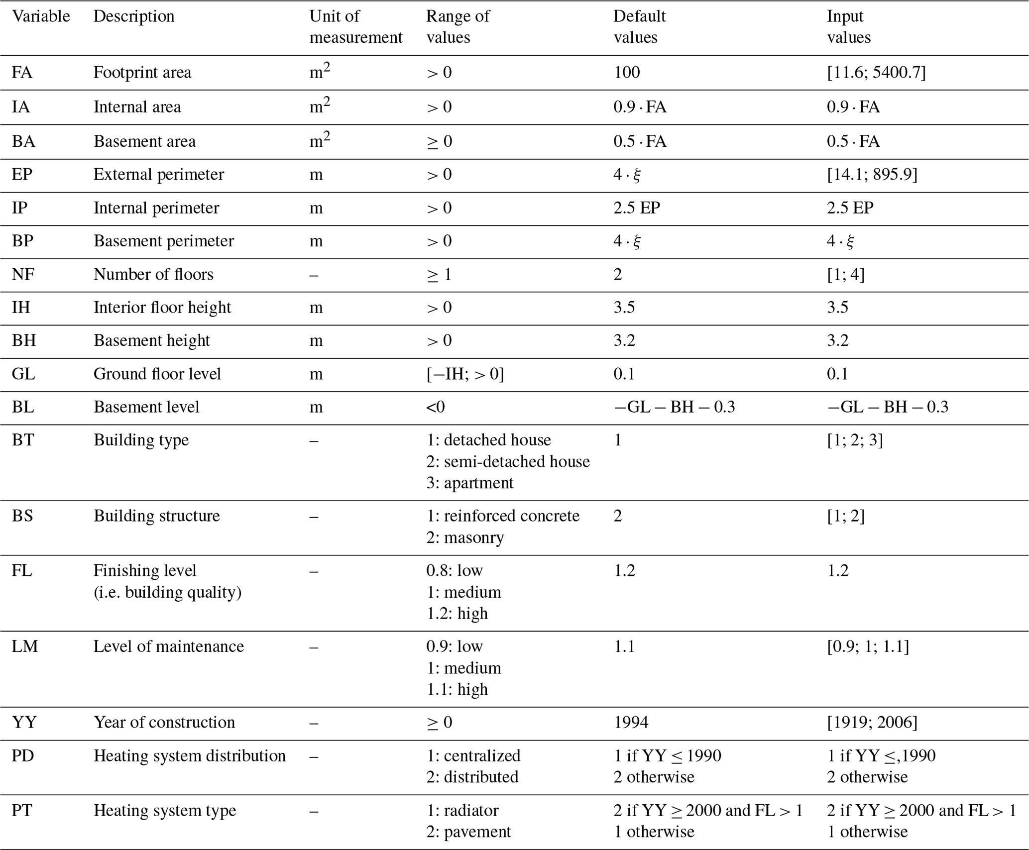
The analysis of the negative effects of different event types on exposed elements is necessary to assess the potential damage of elements at risk. Fundamental to the consequence assessment is the concept of depth–damage functions defined as relations between floodwater depth and corresponding damage. Considering hazard scenarios, the depth–damage functions enable the estimation of expected direct losses, hinged on a spatial representation of flood process patterns and categorized elements at risk (Mazzorana et al., 2014). Although damage functions are generated for a specific building of a given type, they can be assumed as reliable predictors of damage for a group of buildings with similar structural/non-structural characteristics. The probabilistic approach is based on the use of the damage model INSYDE (Dottori et al., 2016a) implemented in the R programming language. The model relies on an analysis of physical damage to buildings considering distinctive land-use classes and building characteristic parameters to derive synthetic damage curves for residential buildings. The INSYDE model can estimate relative damage (i.e. percentage estimation of losses with respect to the total value of the building) and absolute damage, the latter considering the unit prices of cost of damage. Here we decide to express the damage in absolute terms to give the monetary measure using the cost per unit of measure (e.g. square metre) applying the model deterministically (i.e. without considering any source of uncertainty). To calculate the damage, we combine the exposure and vulnerability data described above with the 2014 flood depth scenario and considering three more existing diverse flood depth scenarios assuming return periods of 10, 100 and 500 years derived from 1-D and 2-D hydraulic modelling designed by the Municipality of Milan in 2019 for the Governmental Territorial Plan and the Flood Risk Management Plan (Municipality of Milan, 2019).
We modelled flood damage on residential buildings falling within the study by the following steps.
-
Absolute damage was calculated by obtaining the absolute damage function and the site-specific depth–damage curves for the residential sector.
-
The annual average loss (AAL) and the exceedance probability (i.e. the probability that a certain damage value will be exceeded within a certain return period) for the residential sector were defined. This value is the expense that would occur in any given year if monetary damage from all hazard probabilities and magnitudes was spread out equally over time, representing the full range of hazard magnitudes and offering a more complete picture of monetary impacts.
-
Damage modelling and mapping at mesoscale analysis: new site-specific depth–damage functions are then developed for the residential sector at land-use level. Potential maximum damage values for the residential sector were attributed to each of the Urban Atlas 2018 land-use classes (i.e. other roads and associated land, industrial, commercial, public, military and private units, green urban areas, discontinuous medium urban fabric, discontinuous dense urban fabric, continuous urban fabric).
-
Damage modelling and mapping at microscale analysis: new site-specific depth–damage functions are then developed for the residential sector at building level. Object-based water levels and damage data were integrated with information on building vulnerability considering the most vulnerable buildings falling in classes 1 and 2 (i.e. very high and high vulnerability) as resulting from the heuristic approach. Features and building characteristic parameters used as model input data are shown in the Appendix B. Therefore, we built depth–damage functions for two building category subsets based on structural and non-structural characteristic frequency (see Fig. C1 in the Appendix). In each category, a distinction was made between elements with and without a basement. Here the functions are expressed by coupling the values of flood depth and damage factor (DF). The DFs in the damage curves are intended to span from zero (no damage) to one (maximum damage), through absolute damage value normalization. Finally, absolute damage for each residential building was calculated by dividing total damage by building footprint (EUR m−2), supplying damage for flooded floors including a basement if present and mapped to have spatially distributed information.
4.1 Hazard scenario definitions: source and pathway estimation
4.1.1 Source estimation
Gridded estimates of flood depth were produced for the flood polygons of the event. A first quality check of the output denoted unrealistic values in urban areas, especially in the largest flood area in the Municipality of Milan (2019), with large portions of the city affected by flood depths of 2 m or larger (Fig. 3). This is in contrast with data reported by the media, referring to flood depths in the order of 30 cm. This is caused by the use of a flood polygon obtained by linking point observations and manual reports rather than on a spatially continuous identification, such as those provided by aerial or satellite imagery. In addition, the large degree of urbanization in such an area adds noise to the elevation data and consequently to the estimation of flood depths. Hence, in a following step we recomputed flood depths using a flood polygon where the shape of buildings (Open Street Maps, OSM) was first subtracted. In the resulting product, flood depths are mostly within the foreseen ranges, except for some areas with values above 5 m along viale Fulvio Testi, Viale Zara and via Volturno. These are attributed to the construction of Line 5 of the underground train line of Milan, particularly to the stations named Ca' Granda, Istria, Marche, Zara and Isola, which took place in 2008–2010, at the same time of the survey campaign carried out to produce the DTM through lidar measurements. After filling the holes of the underground stations in the DTM using neighbouring values, resulting flood depths are within realistic ranges, with a mean depth of 19 cm and a 90th percentile of the flooded cells of 42 cm.
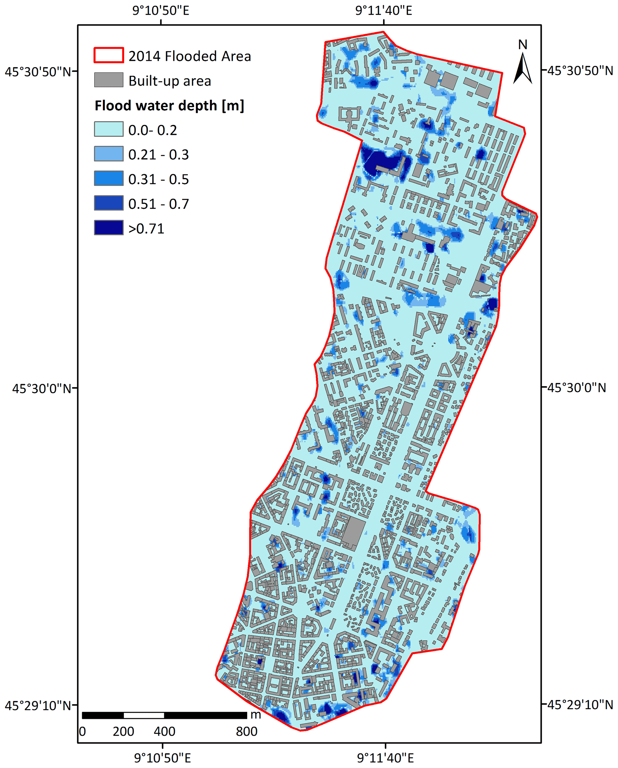
Figure 3Estimated flood depths for the flooded polygon in Milan. Built-up-area shapefile from © OpenStreetMap contributors 2022. Distributed under the Open Data Commons Open Database License (ODbL) v1.0. Base map is from © Regione Lombardia 2022.
4.1.2 Pathway estimation
Sinks and at-risk buildings were identified and mapped (Fig. 4a). A total of 1246 buildings, 81 % of the inundated residential buildings during the 2014 flood event, lie within or adjacent to sink areas where water can potentially pool during a flood and amplify the hazard especially in the case of an inefficient drainage system. Based on Urban Atlas land-use classes 16.1 % of the inundated built-up area was comprised of continuous urban fabric (where 81% presents an average degree of S.L. > 80 %) and 82.8 % of discontinuous urban fabric (where 49 % presents an average degree of S.L. between 50 % and 80 %) (Fig. 4b). Considering the Copernicus Imperviousness Density map resampled at 5 m (Fig. 4c) and building footprint, the NISR has been calculated. Relating NISR to Urban Atlas land-use classes, the most exposed buildings to hazard amplification due to soil sealing fall into continuous (S.L. > 80 %) and discontinuous (S.L. 50 %–80 %) dense urban fabric mostly located in areas with estimated water depth ranging between 0 and 0.20 m during the 2014 flood (Fig. 5).
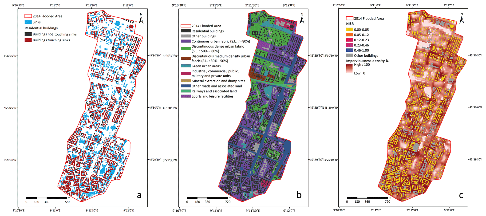
Figure 4(a) Sink distribution map (touching sinks in red; non-touching sinks in grey). (b) Urban Atlas 2018 map (residential buildings in black; other buildings in grey). (c) Copernicus Imperviousness Density map resampled at 5 m and NISR distribution for residential buildings. Built-up-area shapefile is from © OpenStreetMap contributors 2022. Distributed under the Open Data Commons Open Database License (ODbL) v1.0. Base maps in (b) and (c) are from © European Union, Copernicus Land Monitoring Service 2022, European Environment Agency (EEA).
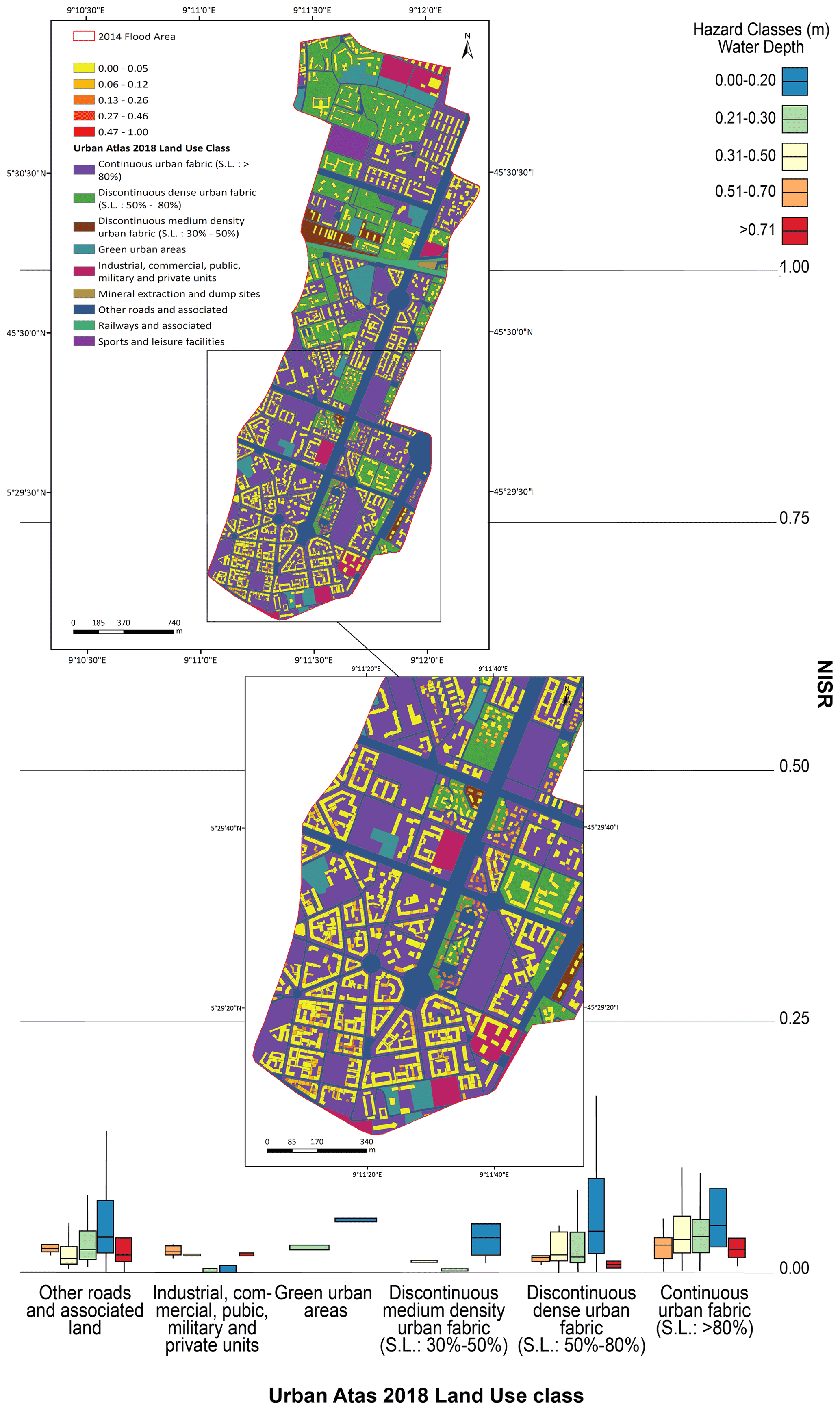
Figure 5Boxplots and maps of NISR distribution for residential buildings according to Urban Atlas 2018 land-use classes and water depth hazard classes. Built-up-area shapefile is from © OpenStreetMap contributors 2022. Distributed under the Open Data Commons Open Database License (ODbL) v1.0. Base map is from © European Union, Copernicus Land Monitoring Service 2022, European Environment Agency (EEA).
4.2 Exposure and structural vulnerability assessment: receptor and consequence estimation
4.2.1 Receptors estimation: heuristic approach
Exposure analysis consisted in the recognition of potentially damaged residential assets (e.g. information on the location, number and type of elements at risk). A total of 1540 residential buildings have been thereby classified and mapped according to structural and non-structural features (Fig. 6), including the attribution of economic values to define building susceptibility (Fig. 6f).
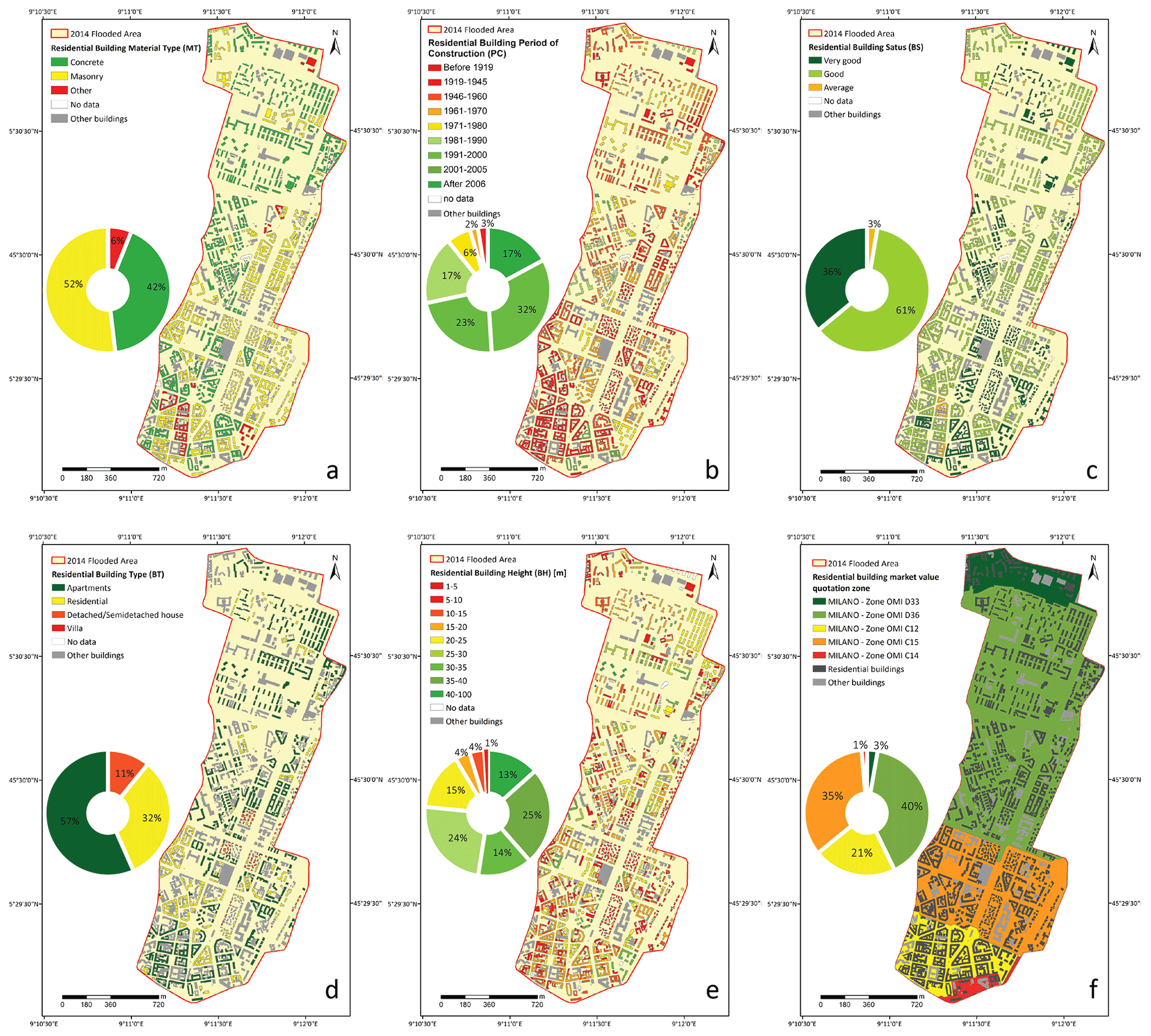
Figure 6Residential Buildings: (a) material type map (MT); (b) period of construction map (PC); (c) building status (BS) map; (d) building type map (BT); (e) building height map (BH); (f) OMI zone map according to the National Real Estate Observatory (OMI) classification based on territory sub-division (central and semi-central urban, suburban, peri-urban, and peripheral areas) having higher market value quotations (increasing from red to green). Pie charts represent the percentages of residential building distribution according to structural and non-structural features. Built-up-area shapefile is from © OpenStreetMap contributors 2022. Distributed under the Open Data Commons Open Database License (ODbL) v1.0. Base map in (f) is from © Geopoi, Map Data 2022.
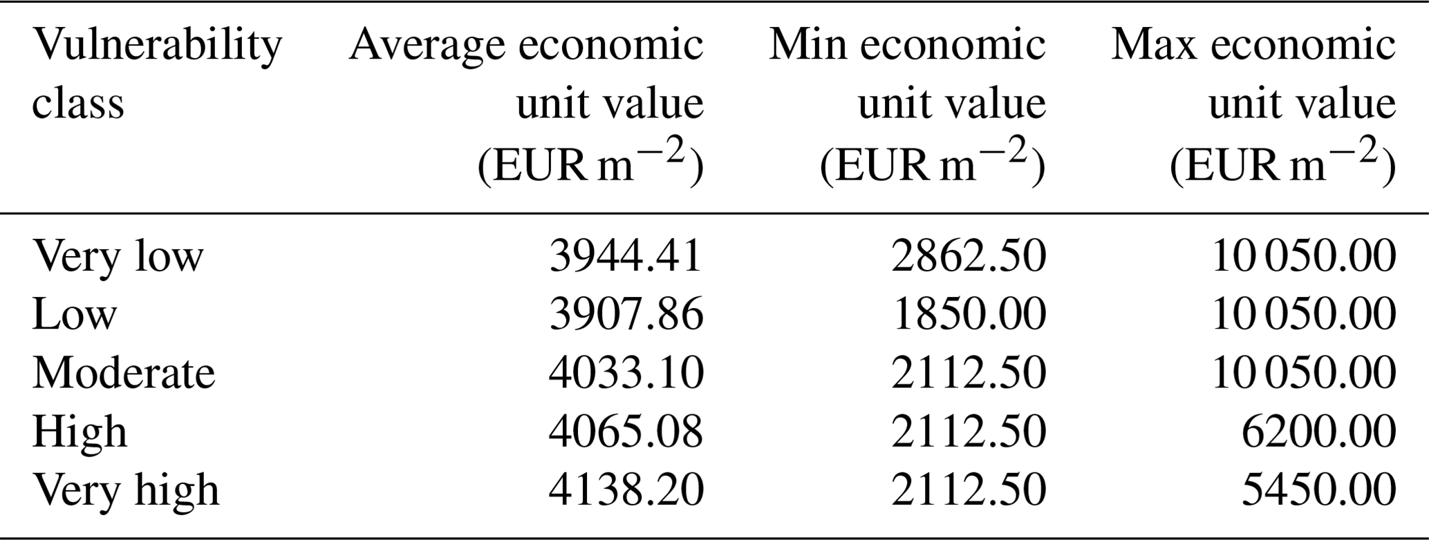
We obtained an info-table of residential buildings classified by hazard values derived by the weighting of hazard classes on the base of flood depth thresholds, sink map and NISR values, as well as total weights derived by structural and non-structural feature weighting. The total score varies from 9 to 34, showing distinct building response capacity against flooding. Low total score values stand for lower building response capacity or missing data. On the basis of the obtained total score, a residential building's structural vulnerability is defined and mapped (Fig. 7a), distinguishing five classes (i.e. very low, low, moderate, high, very high) and including the economic unit value based on their relative market value quotation (EUR m−2). A total of 81 residential buildings fall in class 1 (0–17), 333 residential buildings fall in class 2 (18–20), 432 residential buildings fall in class 3 (21–23), 477 residential buildings fall in class 4 (24–27), and 217 residential buildings fall in class 5 (28–39) (Fig. 7a). For 415 buildings falling in the most vulnerable classes (i.e. classes 1 and 2, “very high” and “high” respectively), 185 buildings are characterized by the presence of a basement (Fig. 7d). Results show that the most vulnerable buildings are mostly located in the southern highly urbanized part of the affected area, closer to the city centre, i.e. zone OMI C12 and C14. Calculating the average relative market value quotation for each vulnerability class, we observed that the residential buildings falling in class “very high” showed the highest average value (i.e. EUR 4148.2 per square metre) (Table 4).

Figure 7(a) Residential building maps classified by vulnerability class and frequency; (b) the most vulnerable residential buildings with and without a basement map; examples of residential buildings falling in classes high and very high (c) without a basement and (d) with a basement respectively and (e) their location. Built-up-area shapefile is from © OpenStreetMap contributors 2022. Distributed under the Open Data Commons Open Database License (ODbL) v1.0. Building pictures are from © Google Maps 2022.
Table 4The average, minimum and maximum economic unit value for each residential building structural vulnerability class.
4.2.2 Consequence estimation: probabilistic approach
To calculate the damage we combine the exposure and vulnerability data described above with the 2014 flood water depth assuming return periods of 500, 100 and 10 years (Fig. 8).

Figure 8Estimated water depth and probability of flooding assuming return period scenarios of (a) 500, (b) 100 and (c) 10 years derived from 1-D and 2-D hydraulic modelling designed by the Municipality of Milan in 2019 for the Governmental Territorial Plan and the Flood Risk Management from © Regione Lombardia 2022. Built-up-area shapefile is from © OpenStreetMap contributors 2022. Distributed under the Open Data Commons Open Database License (ODbL) v1.0.
Firstly, absolute damage has been calculated obtaining a damage function for the residential sector. The resulting total absolute damage to residential properties is equal to EUR 105.3 million, EUR 100.8 million and EUR 93 million, assuming return periods of 500, 100 and 10 years respectively and EUR 62.4 million for the 2014 flood. It is noteworthy that here the modelled absolute damage values for the considered return periods are always greater than the 2014 event values (Fig. 9a). As can be seen by observing the depth–damage functions for the residential sector, the shape of the damage for the 2014 flood is steeper until 0.2 m water depth than other functions because the most vulnerable buildings fell within the 0.26–0.50 m class. Nearly maximum damage occurs when water depths exceed 0.5 m. The three flood scenarios' functions reach their maximum between 1.5 and 2 m (Fig. 9b). The obtained AAL corresponds to EUR 18.3 million, whilst the events with the lowest annual exceedance probability are associated with the highest total damage, showing that as probability decreases, damage increases (Fig. 9c). As a third step, collected data for each inundated building in Milan were used for developing a site-specific mesoscale depth–damage curve for the residential sector (Fig. 10) and mapping (Fig. 11). At mesoscale the absolute damage result for each Urban Atlas 2018 land-use class was higher for the “continuous urban fabric (S.L.: > 80 %)” class for all flood scenarios and for the 2014 flood likewise (Fig. 10e). The function for the “continuous urban fabric (S.L.: > 80 %)” runs up to EUR 54.3 million, considering the 500-year return period scenario (Fig. 10c) being steeper in the first metre according to the literature (Jongman et al., 2012; Huizinga et al., 2017; Scorzini et al., 2022). As can be seen, the shape of the damage for the “continuous urban fabric (S.L.: > 80 %)” is similar for the return period scenarios of 500 (Fig. 10c) and 100 years (Fig. 10b), whereas for the 10-year return period scenario (Fig. 10a) and for the 2014 flood (Fig. 10d), the functions are much steeper in the first metre and in the first 0.2 m of water depth respectively, being characterized by areas affected by low flood depth (less than 0.2–0.5 m). Therefore, the second highest maximum damage values are found for those residential buildings falling within “other roads and associated land” land-use class with functions running up to maxima of EUR 27 million considering the 500-year return period scenario, reaching its maximum at about 2.5 m of water depth (Fig. 10c).
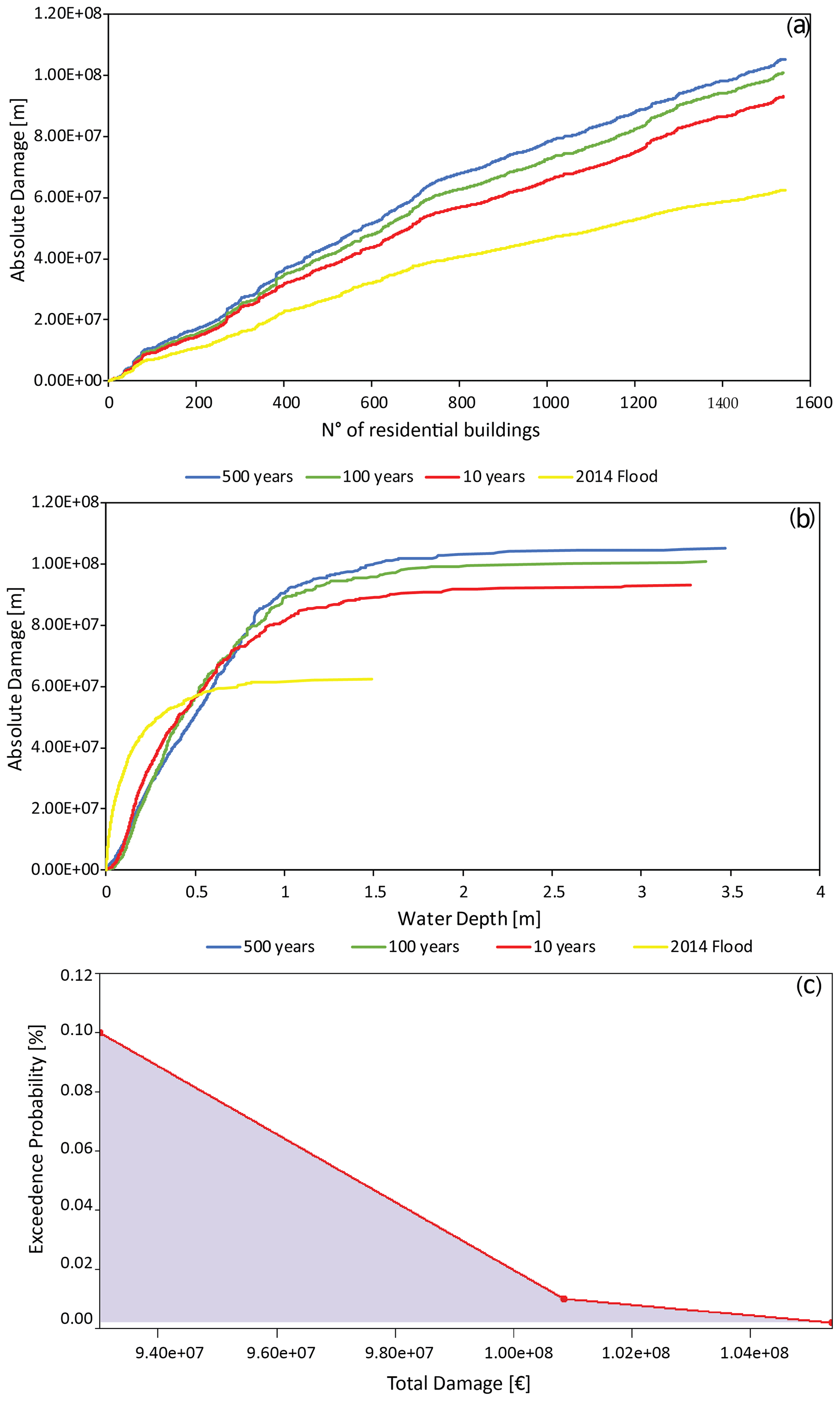
Figure 9(a) Absolute damage for the residential sector (no. of buildings) considering return periods of 500, 100 and 10 years and the 2014 flood event; (b) site-specific depth–damage curve for the residential sector considering the return periods of 500, 100 and 10 years and the 2014 flood event; (c) exceedance probability of absolute damage for the residential sector.
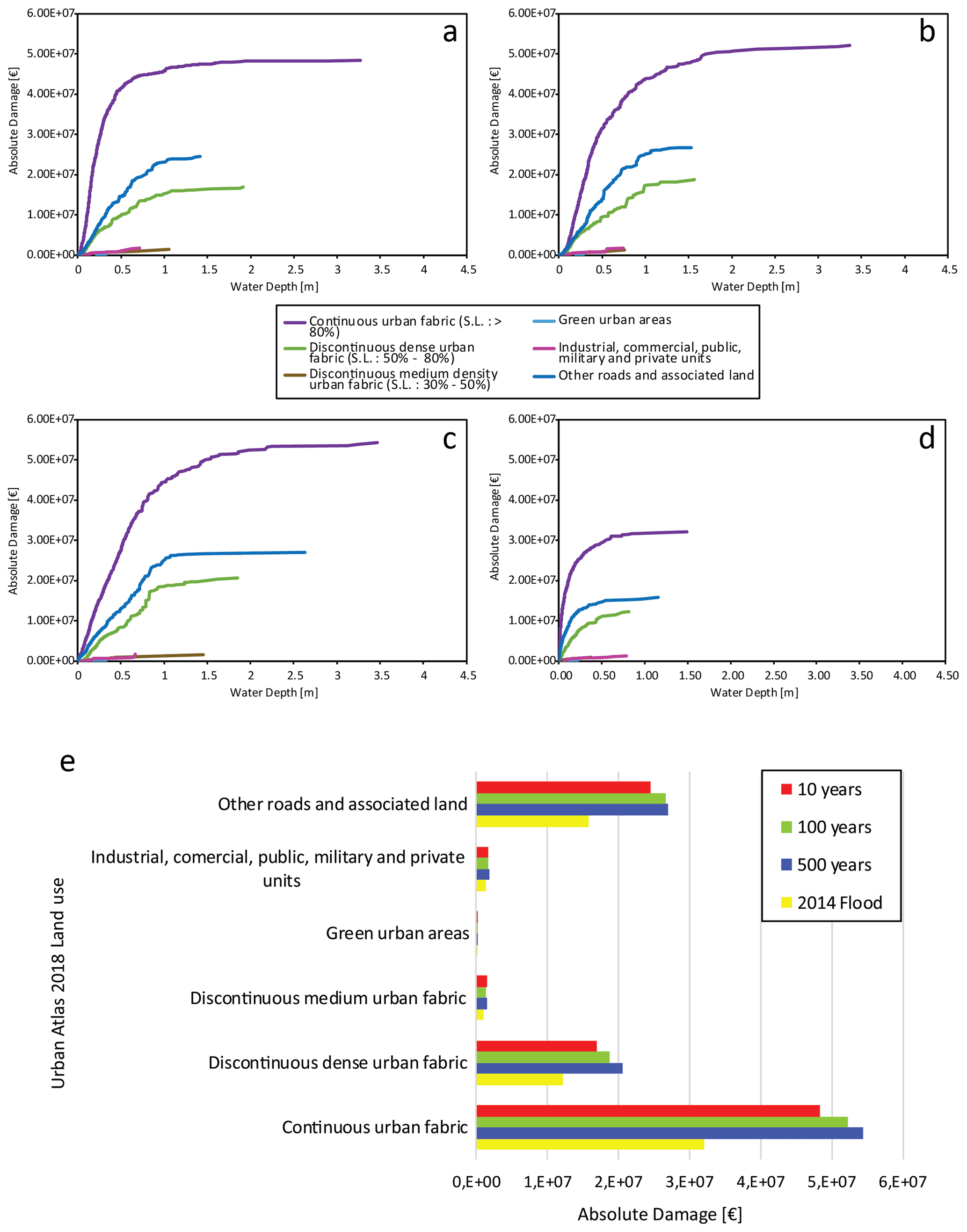
Figure 10Site-specific mesoscale depth–damage curves for the residential sector. The x axis represents the inundation depth, and the y axis represents the damage fraction corresponding to the inundation depth for a specific land-use class assuming return periods of (a) 10, (b) 100 (c) 500 years and (d) 2014 flood. (e) Comparison of total absolute damage distribution at mesoscale.
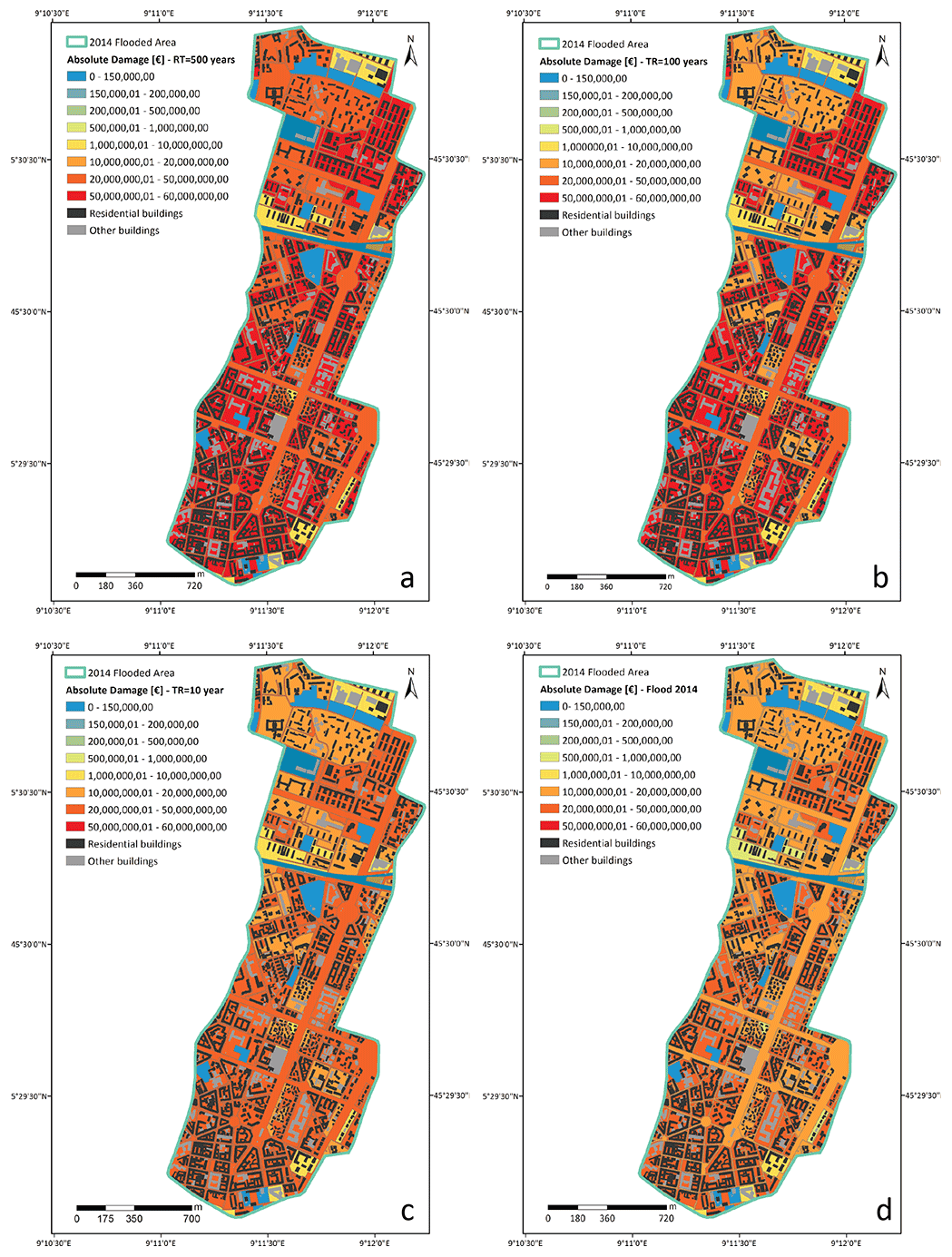
Figure 11Mesoscale absolute damage mapping considering return periods of (a) 500, (b) 100 and (c) 10 years and (d) the 2014 flood event for Urban Atlas 2018 land-use classes. Built-up-area shapefile is from © OpenStreetMap contributors 2022. Distributed under the Open Data Commons Open Database License (ODbL) v1.0. Base maps are from © European Union, Copernicus Land Monitoring Service 2022, European Environment Agency (EEA).
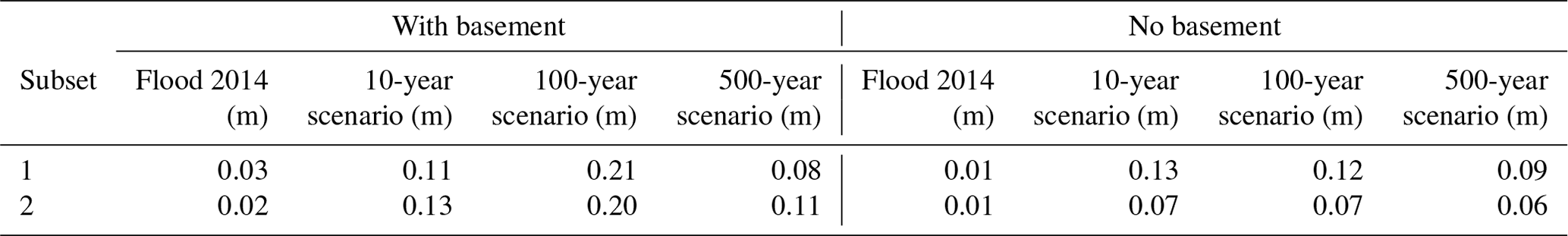
A more detailed, microscale analysis was then performed integrating object-based water levels and damage data with information on building vulnerability focusing on the most vulnerable buildings falling in classes 1 and 2 (i.e. very high and high vulnerability), as resulting from the heuristic approach. Specifically we built site-specific microscale depth–damage curves for two building category subsets based on the frequency distribution of structural and non-structural indicators (Appendix C), making a distinction between elements with and without a basement: (1) BT = “detached and semi-detached house”; MT = “masonry”; BS = “good”; NISR = “0.05–0.12”; BH = 1–5 m; PC = 1919–1966; (Fig. 12a); (2) BT = “detached and semi-detached house”; MT = “concrete”; BS = “good”; NISR = “0.05–0.12”; BH = 1–5 m; PC = 1919–1966 (Fig. 12b). Considering the first subset the shape of the damage for the buildings with a basement are not similar; notably the function for the 10-year return period scenario is much steeper in the first 4 m of water depth. The function for the 2014 flood is much steeper in the first 0.20 m of water depth, albeit its maximum value remains lower compared to the other flood scenarios. Considering the buildings without a basement, the shape of the damage functions for the 10- and 100-year return period scenarios are quite similar, as the functions are much steeper in the first 0.5 m of water depth. However, the difference with the 500-year return period becomes significant after the flooding depth exceeds 1 m. The function for the 2014 flood is much steeper in the first 0.30 m of water depth, although its maximum value remains lower compared to the other flood scenarios (Fig. 12a). Figure 12b shows the function for the 2014 flood of the buildings with a basement to be much steeper in the first 0.30 m of water depth. Nearly maximum damage occurs when water depths exceed 0.3 m. As one can see, the shape of the damage curve for the 500-year return period differs significantly, as the function is less steep, albeit it reaches higher maximum damage values at about 1.5 m. Looking at the buildings without a basement, the shape of the damage functions for the 10- and 100-year return period scenarios are quite similar to the 2014 flood and the 500-year return period scenario. The latter functions are much steeper in the first 0.20 m of water depth (Fig. 12b). Table 5 compares the flood depths for causing a DF equal to 0.1 for the two residential building subsets. In each subset, a distinction was made between elements with and without a basement. Spatial distribution and variability are finally obtained by mapping absolute damage for each residential building calculated by dividing total damage by building footprint (EUR m−2) (Fig. 13).
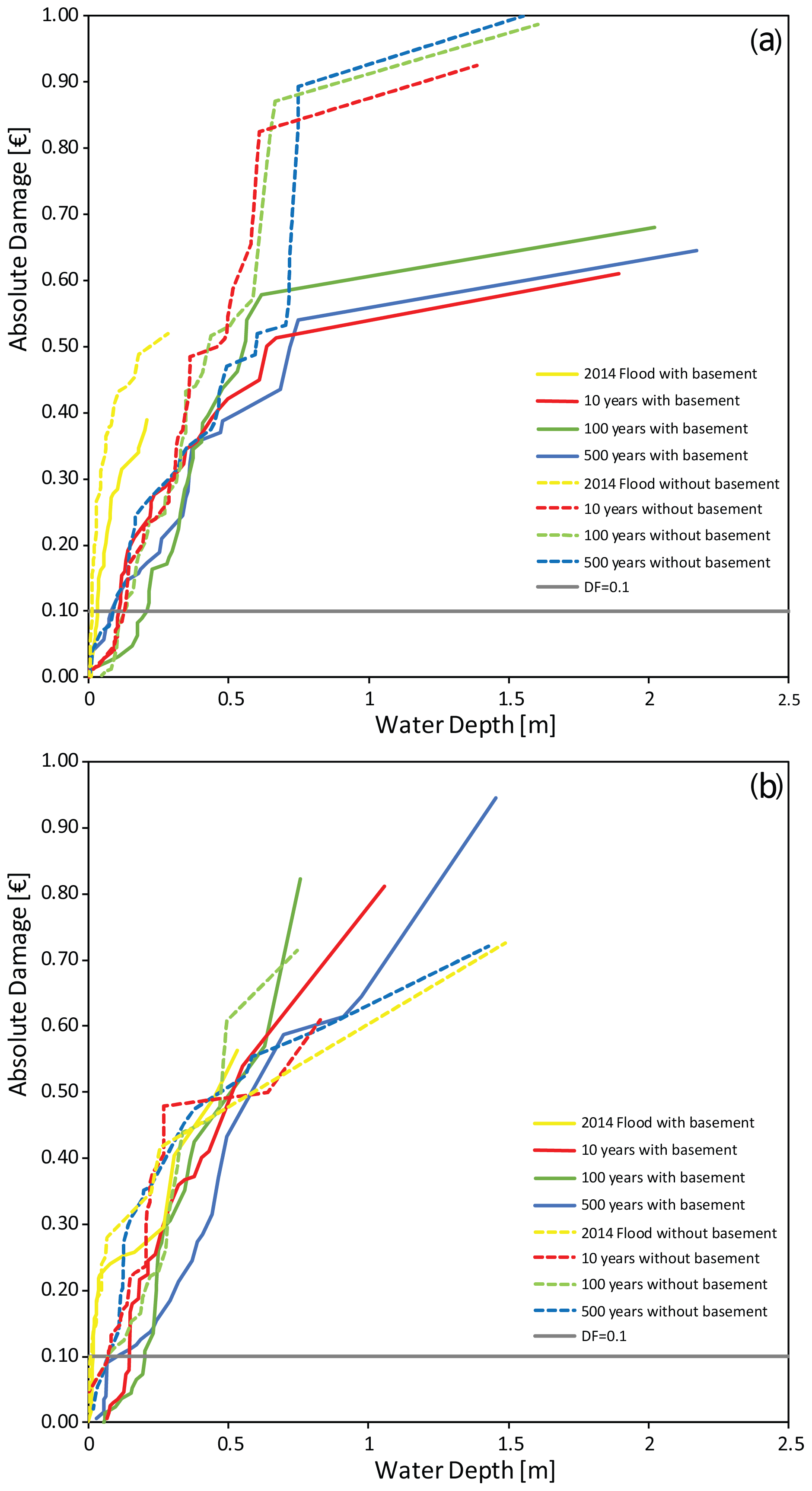
Figure 12Site-specific microscale depth–damage curves for the residential sector for the 2014 flood (yellow lines) and return period scenarios of 10 (red lines), 100 (green lines) and 500 (blue lines) years for buildings falling in the most vulnerable classes (i.e. classes 1 and 2, “very high” and “high”): (a) BT = “detached and semi-detached house”; MT = “masonry”; BS = “good”; NISR = “0.05–0.12”; BH = 1–5 m; PC = 1919–1966 with a basement (solid line) and without a basement (dashed lines); (b) BT = “detached and semi-detached house”; MT = “concrete”; BS = “good”; NISR = “0.05–0.12”; BH = 1–5 m; PC = 1919–1966 with a basement (solid line) and without a basement (dashed lines). Solid horizontal grey line stands for DF equal to 0.1.
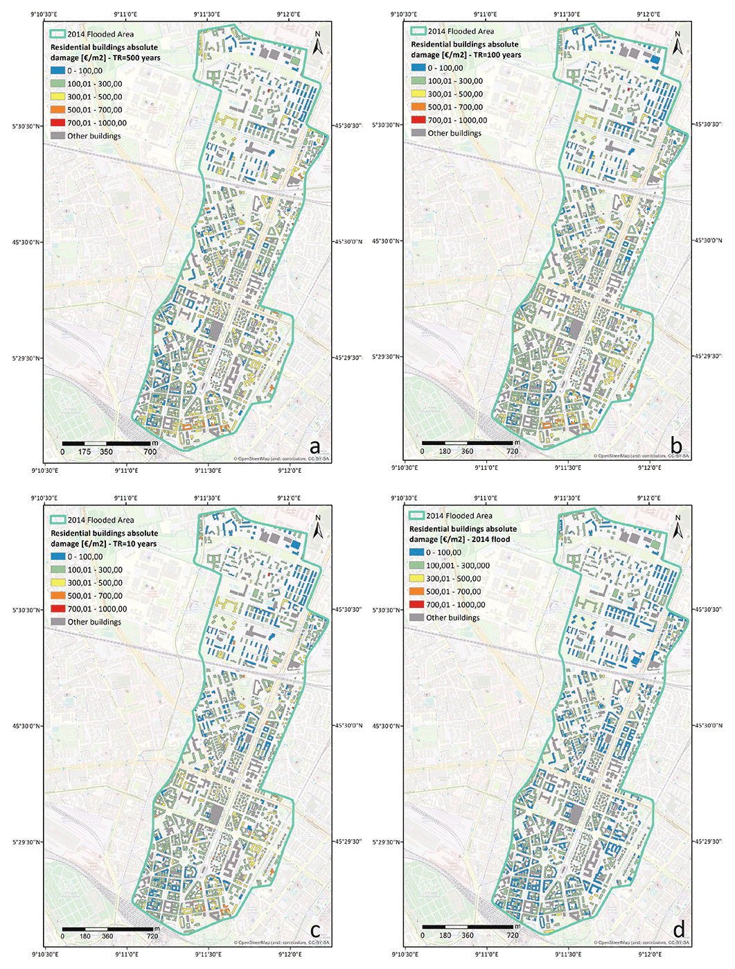
Figure 13Microscale absolute damage mapping considering return period scenarios of (a) 500, (b) 100 and (c) 10 years and (d) the 2014 flood event for the two most vulnerable building category subsets. Base maps and built-up-area shapefile are from © OpenStreetMap contributors 2022. Distributed under the Open Data Commons Open Database License (ODbL) v1.0.
Table 5Flood depths necessary for causing a DF equal to 0.1, according to the two building type subsets.
In this study we described the development and the application of a quantitative method based on the causal chain of the SPRC focusing on structural vulnerability assessment as a fundamental and dynamic component of flood risk analysis in urban areas. We consider high vulnerability and exposure the outcome of skewed development processes, such as those associate with the intensity of extreme and non-extreme climate and weather events, morphological features, buildings' structural and non-structural characteristics, and land use frequently associated with rapid urbanization and suburbanization as for large metropolitan regions. Moreover, vulnerability can be seen as situation-specific and scale-dependent, interacting with a hazard event to generate risk. Therefore, the capacity for risk prevention and reduction may be understood as a series of elements, measures and tools directed toward intervention in hazards and vulnerabilities with the objective of reducing existing or controlling future possible risks (Cardona, 2004) at diverse scales of analysis. We characterized flood hazard intensity on the basis of variability in water depth during a recent event and spatial exposure also as a function of buildings' surroundings and buildings' intrinsic characteristics as a determinant factor of the element-at-risk susceptibility and response capacity. In this sense the use of the chosen vulnerability indicators and a geographic scale sufficient to depict spatial differences in vulnerability from land use to building level allow us to identify structural vulnerability hotspots and to inform depth–damage curves for calculating potential damage. Empirical measures of the 2014 flood event enabled a valid characterization of the hazard system and the intrinsic, underlying relationships and interdependencies required in the structural vulnerability assessment framework.
5.1 Hazard scenario definitions: source and pathway estimation
Starting with source estimation, we reassessed the 2014 flood characteristics in a densely urbanized area of Milan, obtaining flood depth values within the foreseen ranges, which are worthwhile data for the study of highly flood-prone residential buildings. This requires knowledge about how the source interactions with the natural and non-natural environment lead to the amplification or the reduction of hazards. The methodology used produces accurate estimates of the flood characteristics, with mean error in flood depth estimation in the range 0.2–0.3 m (Cohen et al., 2019). Yet it enables realistic representation of the flood extent, with robust performance. Furthermore, it is scalable to larger domains and particularly suitable for coupling with satellite-derived flood extents. In contrast, applications in urban areas are especially challenging and may need manual fine-tuning to overcome a range of issues coming from the flood characteristics, elevation data, building size and underground structures, among others. Indeed, the environment offers resources for human development at the same time as it represents exposure to intrinsic and fluctuating hazardous conditions (Lal et al., 2012). Between 2012 and 2018 in the Milan metropolitan region, 58 % of land-use changes concern the urban expansion uptake of agricultural areas (Copernicus Programme, 2018). Thus, we estimated the pathway analysing land use, focusing on residential built-up areas and identifying low-lying and impervious surfaces (Fig. 4c). In this zone low-lying areas are already affected by periodic flooding after heavy rainfall, and greater urbanization and sprawl could exacerbate this problem. Thus, buildings adjacent or close to these areas are considered at greater risk of being flooded (Fig. 4a). As is evident from the results higher NISR values fall within low-lying areas. However, these no longer coincide with higher values of water depth recorded for the 2014 flood event (Fig. 5). Therefore, in areas that are already developed, sink maps and NISR classes can be used to prioritize areas for better risk mitigation planning purposes.
5.2 Exposure and structural vulnerability assessment: receptor and consequence estimation
By assessing the exposure we defined the receptors and consequently how vulnerability varies spatially. The heuristic approach incorporates residential building exposure categories, sources and pathway estimation outputs, meeting the need to achieve a fast, though approximate, vulnerability estimation at building level (Fig. 7). The majority of the residential buildings fall in classes “low” and “moderate” (Fig. 7a). Moreover, residential buildings falling in classes “high” and “very high” are mostly houses built of masonry between 1919 and 1970 in a good state of maintenance, of which most have a basement, and the highest average economic unit value in euros per square metre (EUR m−2; Table 4). These buildings are also located where NISR is higher, demonstrating that it is a valid support for quantifying buildings most exposed to hazard amplification especially in dense urbanized areas (Fig. 4c). The method resulted in being valuable as a preliminary vulnerability indicator-based assessment of the potential weaknesses in the structural building system to be used in the consequence estimation. Consequence estimation relates to the probabilistic phase of the structural vulnerability based on different scales of model application to obtain the AAL, which is a rough measure of the absolute “riskiness” of a set of exposures and refers to the long-term expected losses per year (i.e. averaged over many years), as well as the site-specific depth–damage curves (such as meso- and microscale curves). Overall AAL represents the full range of hazard magnitudes, offering a more complete picture of monetary impacts that should be expected to be incurred over time. Thereby exposed assets as a function of water level were then translated into absolute damage. To calculate the damage we combine the exposure and vulnerability data with the 2014 flood water depth assuming return periods of 10, 100 and 500 years. Flood depths for different return periods show small differences due to the relatively flat area where the floodwaters can spread. Localized spots with flood depths larger than 4 m occur in depressions being filled by the floodwaters (e.g. metro stations, road underpasses). The “continuous urban fabric (S.L.: > 80 %)” class is more affected by low flood depth (less than 0.2–0.5 m) for the 2014 flood and 10-year return period than the other two scenarios (Fig. 10). Nevertheless, at mesoscale the “continuous urban fabric” Urban Atlas 2018 land-use class with the occurrence of at least 80 % of soil sealing shows higher absolute damage values within the first metre according to the existing literature. Besides the DF on built-up areas being different for diverse types of land use (Huizinga et al., 2017; Gabriels et al., 2022), it tends to be steeper within the first metre. Residential buildings falling in the “roads and associated land” class likewise show great absolute damage values. Roads accounted for the increase in impervious cover, having a significant impact on natural water systems by preventing water infiltration (Figs. 11 and 12), whereas lower values of absolute damage measured for those building located close to “green urban areas” are noteworthy (Figs. 11 and 12). At microscale observing the depth–damage functions for the residential sector the shape of the damage for the 2014 flood is steeper to 0.2 m water depth than other functions. Nearly maximum damage occurs when water depths exceed 0.5 m probably because observing the “very high-vulnerability” and “high-vulnerability” building distribution against water depth classes is evident that the most vulnerable buildings fall within the 0.26–0.50 m class. Therefore, we considered two subsets of buildings falling in the most vulnerable classes (i.e. classes 1 and 2, “very high” and “high”) as resulting from the heuristic approach buildings, obtaining site-specific depth–damage curves. Observing Table 5, which compares the flood depths needed for causing a DF equal to 0.1 for the different building types, similar values were found for all buildings “with a basement” for the three flood scenarios, and they increased for buildings “without a basement”. A possible explanation for this might be due to a larger residence time of water and to the “filling effect” occurring in basements. It is important to underline that a DF equal to 0.1 for the 2014 flood is reached at lower values of flood depths for both the subsets, demonstrating that even events with moderate magnitude in terms of flood depth in a complex urbanized area may cause more damage than would be expected.
In general from the findings some key observations emerge.
-
At mesoscale the idea that impervious surfaces amplify flood hazards and cause more relevant direct and tangible damage to structures is reinforced. One consequence of increasing impervious cover in urban areas is that conventional urban storm water systems with underground piping can be overwhelmed when run-off exceeds the capacity of the system and causes surface flooding as for the city of Milan.
-
Structural vulnerability measurements and pattern understanding are improved: we derived where vulnerability occurred and how vulnerability was distributed at local scale in a spatially explicit way, indicating vulnerability hotspots. From the selected list of flood vulnerability indicators, the actual circumstances that determine structural flood vulnerability are site-specific, hazard-dependent and dependent on elements at-risk.
-
New insights were given for the development of site-specific local residential depth–damage curves for a more comprehensive description of residential building damage processes and parameterization across two spatial scales of analysis. Flood damage modelling on the building level is important to optimize investments for the implementation of flood risk management concepts in urban areas.
5.3 Advantages, limitations and future developments
Lombardy, Italy's economic engine, is particularly vulnerable to flood hazard risk, the consequences of which are likely to affect national growth and stability. A better understanding of vulnerability patterns is important for public budgeting, as well as private resilience choices. The study presents several advantages to support decision makers, as planners and policy makers, in improving their investment strategies for the mitigation and the reduction of flood damage but also to improve the currently low flood insurance coverage, exploring new insurance model trials to sustain insurance systems for residential properties (Gizzi et al., 2016). In addition, it helps stakeholders working in emergency planning to set priorities during a flood event by the identification of the most vulnerable buildings due to its intrinsic characteristics. The SPRC model is a valuable tool to support decision makers in better understanding vulnerability drivers, complex processes and their interrelations, acting as a guide for interventions, priority measures and resource allocation either in the pre- or post-event phases. Examples of pre-flood applications of the outputs may include the development of flood hazard mitigation strategies that outline policies and programmes for reducing flood losses, including nature-based solutions or the use of the obtained AAL as an input of a cost-benefit analysis of prevention and mitigation measures. Thereby, examples of post-event applications of the outputs may include the application of land-use planning principles and practices and the allocation of resources for flood-resilient building interventions. Therefore, the use of an indicator-based methodology to inform the depth–damage curve allows users to add indicators according to their needs, priorities and data availability. Herein, besides using only one characteristic of the building, valuable vulnerability building indicators based on structural and non-structural attributes and surrounding characteristics that contribute to the vulnerability of the elements at risk are used to identify vulnerability hotspots. The use of spatially distributed information to obtain vulnerability mapping and related potential damage at land-use and building levels gives useful indications on elements that will most likely experience the impact of a flood event and consequently where and how specific intervention of protection and maintenance or particular insurance against flood damage could be required. Moreover, the use of the environmental feature characteristics to define the building's surroundings in the vulnerability assessment plays an important role in capturing the totality of the landscape elements that influence the vulnerability patterns amplifying or diminishing vulnerability of elements at risk. Nevertheless, some limitations can be noted. A considerable amount of data at local scale is needed; however, it is not always available to the local authorities or cannot be accessible or easily collected. In Italy the current national and regional databases are often of insufficient quality to support a robust analysis. One of the three main elements to be correlated among hazard, vulnerability, and losses are often missing or too hazy to make an appropriate comparison with scientific findings (Molinari et al., 2014). Here effects of hazard interactions on the buildings susceptibility and exposure are hazard-intensity specific based on 2014 flood event severity; however, more empirical data should be included to provide more powerful analytical tools (e.g. vulnerability curves) (Arrighi et al., 2020). Several studies have shown that estimations based on depth–damage functions may be very uncertain since water depth and building use only represent a fraction of the whole data variance (Merz et al., 2004; Fuchs et al., 2019). Therefore, the lack of loss data or scattered information on the damage suffered by buildings does not allow a proper comparative assessment between past flood event damage data and those findings obtained by modelled depth–damage functions. Furthermore, better information on past events and damage occurrence and amount would provide more information regarding the building response capacity, implying detailed event documentation (Fuchs et al., 2019). Thus, the scoring procedure in this study has been done on the basis of the literature having many associated uncertainties. Flood over-prediction can lead to over-engineered schemes for defences (Seenath et al., 2016). A conceivable future development would be to base the scoring procedure on documentation of other available past events occurring in the study area or of future events, collecting and rehabilitating the scattered data on the economic impact of past flood events, including the indemnities paid to insurance policy holders, compensations paid for uninsured residential flood damage and state aid provided to economic entities to foster recovery. As for the latter point, available products and services of the European Copernicus Earth Observation programme can be a valid support to bridge this gap. Specifically, the Copernicus Emergency Management Service could provide information about the damage grade, its spatial distribution and extent (i.e. grading map) derived from images acquired in the aftermath of the flood event. Furthermore, the approach could certainly be broadened to commercial buildings and critical facilities (e.g. schools, hospitals, public buildings) enlarging the dataset and the study area.
The goal of this study was to analyse structural vulnerability patterns to enhance the parameterization of the flood damage assessment model for the residential sector in a flood-prone area. Data associated with past damaging floods have been elaborated for the purpose of evaluating the vulnerability of a portion of the urbanized area of Milan in relation to the flood intensity. At building level structural vulnerability classes were strictly driven by the structural type combined with the construction materials, building age and basement presence. On the basis of the five structural vulnerability classes the economic unit value based on their relative market value quotation describes that the most exposed buildings, mostly located in the southern highly urbanized part of the affected area, are the one with the highest average market value. Besides building attributes, findings indicate that also extrinsic parameters describing the building's surroundings, such as morphological features and land use, indirectly affected vulnerability spatial distribution, highly influencing hazard propagation. Results provide a basis to obtain residential building-scale flood damage estimation and site-specific damage curves and mapping. Decision makers, urban and emergency planners, and users that deal with flood insurance might be potential end users of these curves. Good strategies and actions against disasters should be a result of better understanding of disaster risk; thus understanding where the most vulnerable areas are located considering the level of damage in different parts of the city could have several potential uses, such as
-
to produce a more accurate early warning system (EWS);
-
to accurately define evacuation sites;
-
to prioritize areas for better risk mitigation planning;
-
to improve the currently low flood insurance coverage.
This aspect of the research suggested that our results provide evidence for an integrated flood risk management that should consider the entire flood risk system and the interaction among each process. Once SPRC is determined, such a model can be adopted to
-
characterize vulnerability patterns of urban flood damaging event within the bounds of this study at suitable spatial resolution;
-
evaluate impacts at building and landscape scale as a consequence of human interventions on river basins (e.g. river training, loss of flood plains and retention capacity, the increase in impervious surfaces, large changes in land cover, and intensified land use in particular for the development of settlements);
-
significantly support decision-making processes based on cost efficiency to prioritize effective interventions for flood risk reduction and mitigation boosting the change from the paradigm of flood protection to the paradigm of flood risk management;
-
minimize the flood risk through changing any of the four elements of the conceptual model.
Hazard classes for flood depth on the basis of the level (in m) of inland flooding raster maps were assigned to residential buildings using the ZONAL STAT tool considering the maximum value (i.e. the largest value of all cells in the value raster that belong to the same zone as the output cell) on the basis of flood depth and velocity thresholds used for the hazard classification in the definition of the Lombardy Region Territorial Coordination Plan (Fig. A1).
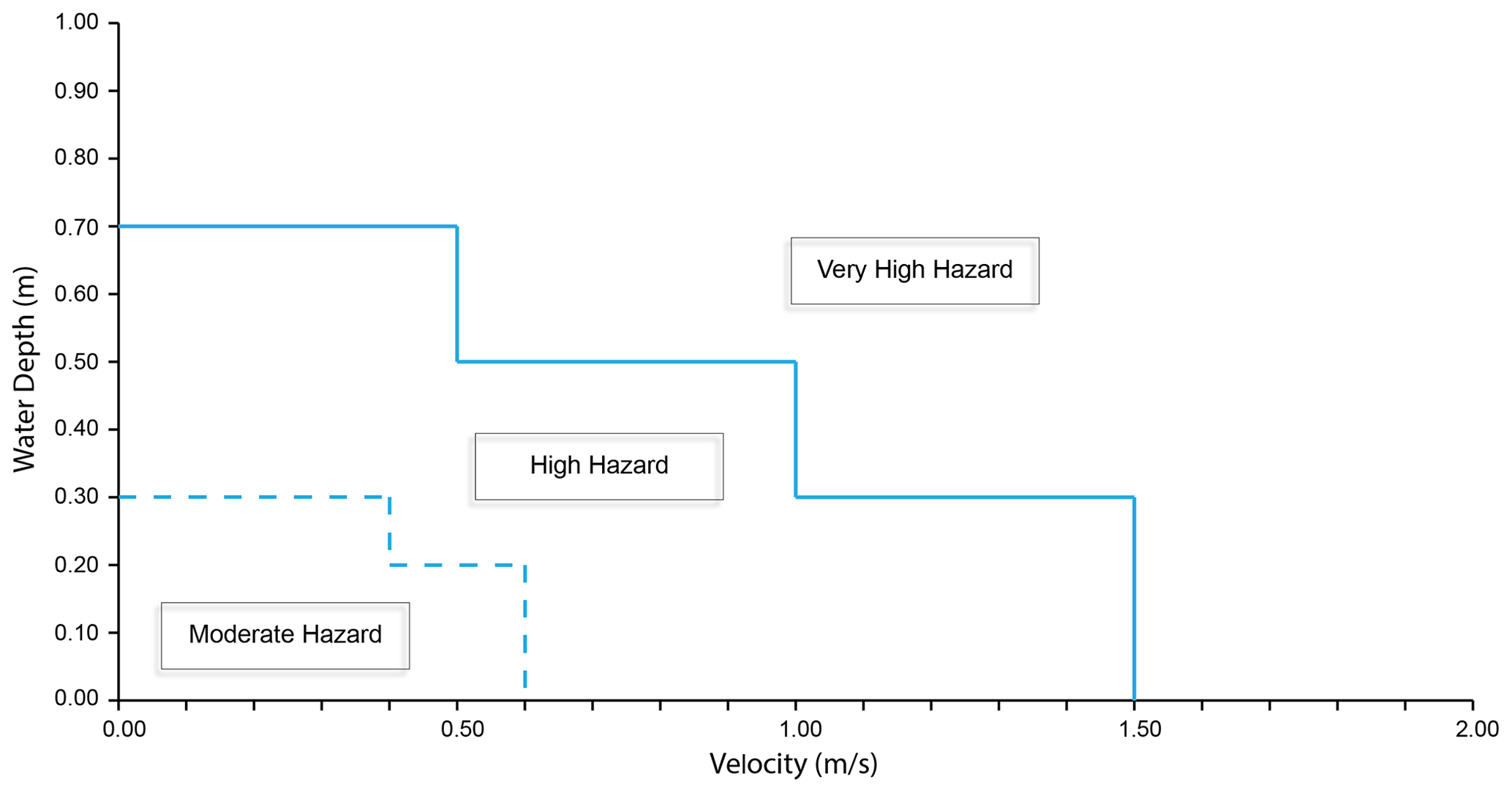
Figure A1Flood depth and velocity thresholds used as reference values for the flood hazard classification (adapted from Lombardy Region PTC).
We assumed default values for missing variables (Tables B1 and B2).
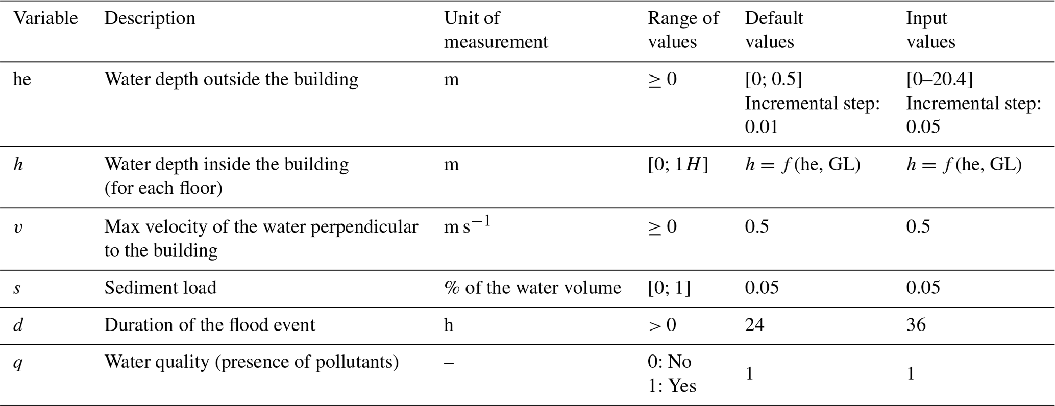
Table B2Building characteristic parameters from the INSYDE model input data.
Structural and non-structural building characteristic frequency distribution has been calculated according to vulnerability classes obtained from the heuristic approach (Fig. C1).
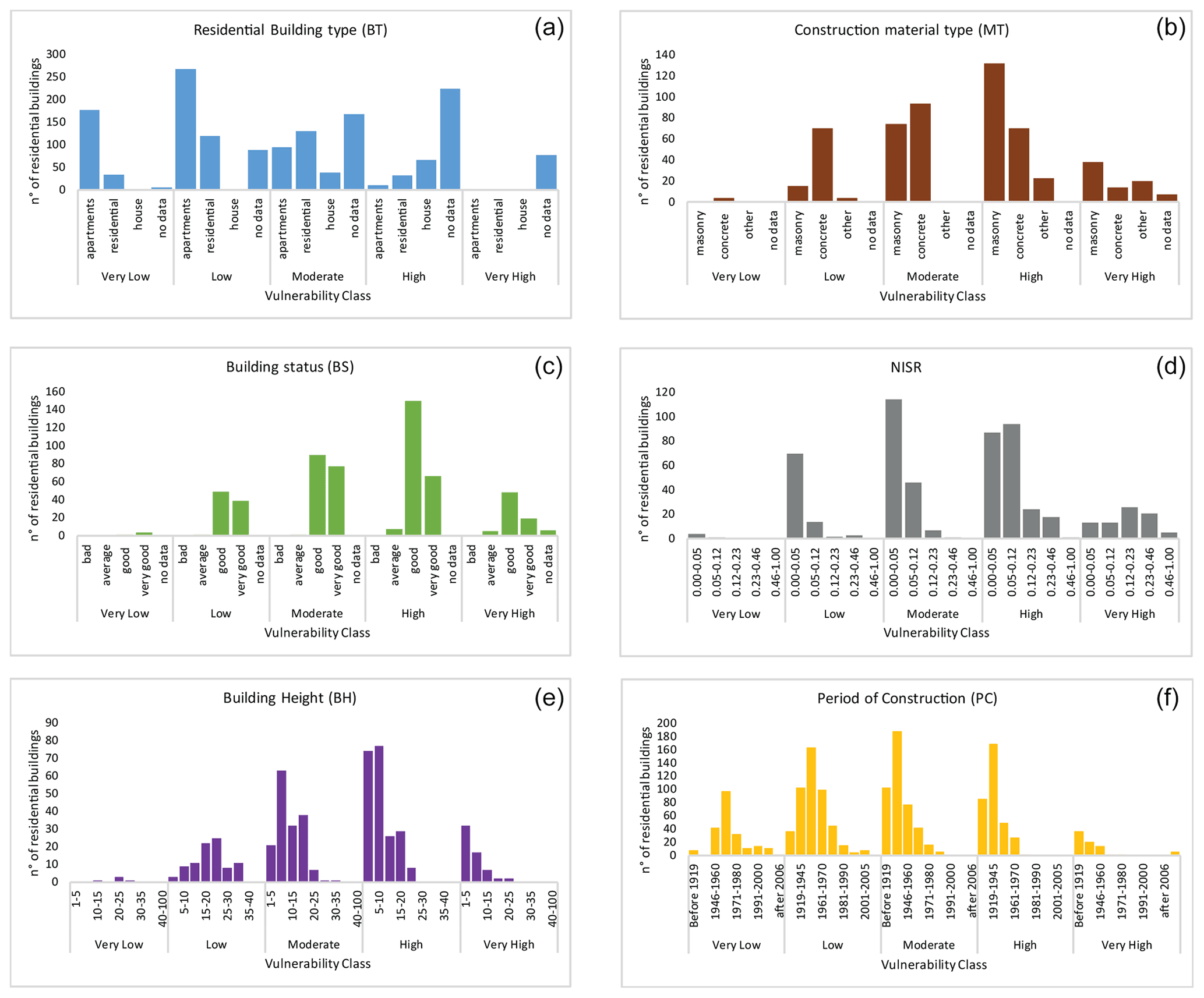
Figure C1Structural and non-structural building characteristic vulnerability class distribution: residential building type (a), construction material type (b), building status (c), normalized imperviousness surface ratio (d), building height (e) and period of construction (f).
Codes (as R code) used to develop depth–damage curves are available at the GitHub repository https://github.com/ruipcfig/insyde (Dottori et al., 2016b).
The Urban Atlas data for 2018 are available at the Copernicus Land Monitoring Service dashboard at https://land.copernicus.eu/local/urban-atlas/urban-atlas-2018?tab=download (European Union, Copernicus Land Monitoring Service, European Environment Agency, 2018a).
The Imperviousness Density 2018 data are available at the Copernicus Land Monitoring Service dashboard at https://land.copernicus.eu/pan-european/high-resolution-layers/imperviousness/ status-maps/imperviousness-density-2018?tab=download (European Union, Copernicus Land Monitoring Service, European Environment Agency, 2018b).
The building height data for 2003 for the Municipality of Milan are available as a Web Map Service (WMS) from the Italian Ministry of the Environment’s Geoportale Nazionale (2003) at http://www.pcn.minambiente.it/mattm/servizio-wms/.
The building status and period of construction data for 2011 for the Municipality of Milan are available from the Italian National Institute for Statistics 2011 census at http://www.istat.it/ (Italian National Institute for Statistics, 2011).
The raster data of the flood depth scenarios with return periods of 10, 100 and 500 years derived from 1-D and 2-D hydraulic modelling for the Municipality of Milan are available at https://www.pgt.comune.milano.it/gall09-relazione-aree-esondabili-e-della-pericolosita/analisi-idraulica-di-dettaglio-download-dati (Municipality of Milan, 2019).
AT supervised and acquired the financial support for the project leading to this publication. EV and MR developed the methodology. MR, LA, SG and IG analysed data and performed the models. MR and IG prepared the manuscript draft with contributions from all co-authors. AT, EV, MR, LA and IG reviewed and edited the manuscript.
The contact author has declared that none of the authors has any competing interests.
Publisher's note: Copernicus Publications remains neutral with regard to jurisdictional claims in published maps and institutional affiliations.
The authors would like to thank the three anonymous reviewers for their careful reading and valuable comments and suggestion.
This research has been supported by EFLIP, a project funded by Fondazione CARIPLO (grant no. 2017-0735).
This paper was edited by Sven Fuchs and reviewed by three anonymous referees.
Akbas, S., Blahut, J., and Sterlacchini, S.: Critical assessment of existing physical vulnerability estimation approaches for debris flows, in: International Conference – Landslide processes: from geomorphological mappingto dynamic modelling, edited by: Malet, J., Remaître, A., and Bogaard, T., CERG Editions, Strasbourg, 229–233, 2009.
Amadio, M., Scorzini, A. R., Carisi, F., Essenfelder, A. H., Domeneghetti, A., Mysiak, J., and Castellarin, A.: Testing empirical and synthetic flood damage models: the case of Italy, Nat. Hazards Earth Syst. Sci., 19, 661–678, https://doi.org/10.5194/nhess-19-661-2019, 2019.
Apel, H., Merz, B., and Thieken, A. H.: Quantification of uncertainties in flood risk assessments, Int. J. River Basin Manag., 6, 149–162, https://doi.org/10.1080/15715124.2008.9635344, 2008.
Arrighi, C., Mazzanti, B., Pistone, F., and Castelli, F.: Empirical flash flood vulnerability functions for residential buildings, SN Appl. Sci., 2, 1–12, https://doi.org/10.1007/s42452-020-2696-1, 2020.
Balica, S. F., Douben, N., and Wright, N. G.: Flood vulnerability indices at varying spatial scales, Water Sci. Technol., 60, 2571–2580, https://doi.org/10.2166/wst.2009.183, 2009.
Becciu, G., Ghia, M., and Mambretti, S.: A century of works on river seveso: From unregulated development to basin reclamation, Int. J. Environ. Impacts Manag. Mitig. Recover., 1, 461–472, https://doi.org/10.2495/ei-v1-n4-461-472, 2018.
Bocci, M., Puppo, D. D., and Fasolini, D.: Il nuovo modello digitale del terreno della Regione Lombardia; un esempio di utilizzo di dati esistenti, XIX Conferenza Nazionale ASITA, 833–841, http://atti.asita.it/ASITA2015/Autori/56.html (last access: 27 April 2022), 2015.
Bouwer, L. M., Bubeck, P., and Aerts, J. C. J. H.: Changes in future flood risk due to climate and development in a Dutch polder area, Global Environ. Change, 20, 463–471, https://doi.org/10.1016/j.gloenvcha.2010.04.002, 2010.
Cammerer, H. and Thieken, A. H.: Historical development and future outlook of the flood damage potential of residential areas in the Alpine Lech Valley (Austria) between 1971 and 2030, Reg. Environ. Change, 13, 999–1012, https://doi.org/10.1007/s10113-013-0407-9, 2013.
Cammerer, H., Thieken, A. H., and Verburg, P. H.: Spatio-temporal dynamics in the flood exposure due to land use changes in the Alpine Lech Valley in Tyrol (Austria), Nat. Hazards, 68, 1243–1270, https://doi.org/10.1007/s11069-012-0280-8, 2013.
Cardona, O. D.: The need for rethinking the concepts of vulnerability and risk from a holistic perspective: A necessary review and criticism for effective risk management, in: Mapping Vulnerability Disasters, Development and People, edited by: Bankoff, G. Frerks, G., and Hilhorst, D., 1st ed., Routledge, London, UK, 37–51, https://doi.org/10.4324/9781849771924, 2004.
Carrera, L., Standardi, G., Bosello, F., and Mysiak, J.: Assessing direct and indirect economic impacts of a flood event through the integration of spatial and computable general equilibrium modelling, Environ. Model. Softw., 63, 109–122, https://doi.org/10.1016/j.envsoft.2014.09.016, 2015.
Cohen, S., Raney, A., Munasinghe, D., Loftis, J. D., Molthan, A., Bell, J., Rogers, L., Galantowicz, J., Brakenridge, G. R., Kettner, A. J., Huang, Y.-F., and Tsang, Y.-P.: The Floodwater Depth Estimation Tool (FwDET v2.0) for improved remote sensing analysis of coastal flooding, Nat. Hazards Earth Syst. Sci., 19, 2053–2065, https://doi.org/10.5194/nhess-19-2053-2019, 2019.
Copernicus Programme: Mapping Guide v6.1 for an European Urban Atlas, 42 pp., https://land.copernicus.eu/user-corner/technical-library/urban_atlas_2012_2018_mapping_guide_v6-1.pdf (last access: 21 May 2021), 2018.
Corradi, J., Salvucci, G., and Vitale, V.: Analisi della vulnerabilità sismica dell’edificato italiano: tra demografia e “domografia” una proposta metodologica innovativa, Ingenio, 1–22, https://www.ingenio-web.it/4518-tra-demografia-e-domografia-una-propostametodologica-innovativa-per-valutare-la-vulnerabilita-sismica-delledificato-italiano (last access: 21 May 2021), 2015.
Crigg, N. S. and Helweg, O. J.: State-of-the-Art of Estimating Flood Damage in Urban Areas, Am. Wat. Res., 11, 379–390, 1975.
Davies, R.: Seveso River Floods Milan, http://floodlist.com/europe/seveso-river-floods-milan (last access: 17 December 2020), 2014.
Department Of The Army and U.S. Army Corps of Engineers (USACE): ER 1105-2-101_Risk Assessment for Flood Risk Management, https://www.publications.usace.army.mil/Portals/76/Users/182/86/2486/ER 1105-2-101_Clean.pdf (last access: 27 April 2022), 2019.
Dietrich, W. E. and Perron, J. T.: The search for a topographic signature of life, Nature, 439, 411–418, https://doi.org/10.1038/nature04452, 2006.
Dodov, B. A. and Foufoula-Georgiou, E.: Floodplain morphometry extraction from a high-resolution digital elevation model: a simple algorithm for regional analysis studies, IEEE Geosci. Remote S., 3, 410–413, https://doi.org/10.1109/LGRS.2006.874161, 2006.
Dottori, F., Figueiredo, R., Martina, M. L. V., Molinari, D., and Scorzini, A. R.: INSYDE: a synthetic, probabilistic flood damage model based on explicit cost analysis, Nat. Hazards Earth Syst. Sci., 16, 2577–2591, https://doi.org/10.5194/nhess-16-2577-2016, 2016a.
Dottori, F., Figueiredo, R., Martina, M. L. V., Molinari, D., and Scorzini, A. R.: INSYDE, a synthetic, probabilistic flood damage model based on explicit cost analysis, GitHub [code], https://github.com/ruipcfig/insyde (last access: 17 May 2022), 2016b.
Elmer, F., Thieken, A. H., Pech, I., and Kreibich, H.: Influence of flood frequency on residential building losses, Nat. Hazards Earth Syst. Sci., 10, 2145–2159, https://doi.org/10.5194/nhess-10-2145-2010, 2010.
Englhardt, J., de Moel, H., Huyck, C. K., de Ruiter, M. C., Aerts, J. C. J. H., and Ward, P. J.: Enhancement of large-scale flood risk assessments using building-material-based vulnerability curves for an object-based approach in urban and rural areas, Nat. Hazards Earth Syst. Sci., 19, 1703–1722, https://doi.org/10.5194/nhess-19-1703-2019, 2019.
European Union, Copernicus Land Monitoring Service, European Environment Agency: Urban Atlas 2018, European Union, Copernicus Land Monitoring Service, European Environment Agency (EEA) [data set], https://land.copernicus.eu/local/urban-atlas/urban-atlas-2018?tab=download (last access: 27 April 2022), 2018a.
European Union, Copernicus Land Monitoring Service, European Environment Agency: Imperviousness Density 2018, European Union, Copernicus Land Monitoring Service, European Environment Agency (EEA) [data set], https://land.copernicus.eu/pan-european/high-resolution-layers/imperviousness/status-maps/imperviousness-density-2018?tab=download (last access: 27 April 2022), 2018b.
Faella, C. and Nigro, E.: Dynamic impact of the debris flows on the constructions during the hydrogeological disaster in Campania-1998: Failure mechanical models and evaluation of the impact velocity, in: Proceedings of the international conference on FSM, Naples, Italy, 179–186, 2003.
Fekete, A., Damm, M., and Birkmann, J.: Scales as a challenge for vulnerability assessment, Nat. Hazards, 55, 729–747, https://doi.org/10.1007/s11069-009-9445-5, 2010.
Figueiredo, R. and Martina, M.: Using open building data in the development of exposure data sets for catastrophe risk modelling, Nat. Hazards Earth Syst. Sci., 16, 417–429, https://doi.org/10.5194/nhess-16-417-2016, 2016.
Fleming, G.: Learning to live with rivers—the ICE's report to government, Proc. Inst. Civ. Eng.-Civ. Eng., 150, 15–21, https://doi.org/10.1680/cien.2002.150.5.15, 2002.
Fuchs, S., Keiler, M., Ortlepp, R., Schinke, R., and Papathoma-Köhle, M.: Recent advances in vulnerability assessment for the built environment exposed to torrential hazards: Challenges and the way forward, J. Hydrol., 575, 587–595, https://doi.org/10.1016/j.jhydrol.2019.05.067, 2019.
Gabriels, K., Willems, P., and Van Orshoven, J.: A comparative flood damage and risk impact assessment of land use changes, Nat. Hazards Earth Syst. Sci., 22, 395–410, https://doi.org/10.5194/nhess-22-395-2022, 2022.
Gizzi, F. T., Potenza, M. R., and Zotta, C.: The Insurance Market of Natural Hazards for Residential Properties in Italy, Open J. Earthq. Res., 5, 35–61, https://doi.org/10.4236/ojer.2016.51004, 2016.
Hallegatte, S., Green, C., Nicholls, R. J., and Corfee-Morlot, J.: Future flood losses in major coastal cities, Nat. Clim. Change, 3, 802–806, https://doi.org/10.1038/nclimate1979, 2013.
Hufschmidt, G., Crozier, M., and Glade, T.: Evolution of natural risk: research framework and perspectives, Nat. Hazards Earth Syst. Sci., 5, 375–387, https://doi.org/10.5194/nhess-5-375-2005, 2005.
Huizinga, J., De Moel, H., and Szewczyk, W.: Global flood depth-damage functions: Methodology and the database with guidelines, EUR 28552 EN, Publications Office of the European Union, Luxembourg, ISBN 978-92-79-67781-6, https://doi.org/10.2760/16510, 2017.
Italian Ministry of Environment’s Geoportale Nazionale: Edificato dei capoluoghi di provincia, Italian Ministry of Environment’s Geoportale Nazionale [data set], http://www.pcn.minambiente.it/mattm/servizio-wms/ (last access: 21 May 2021), 2003.
Italian National Institute for Statistics: 2011 census, Italian National Institute for Statistics [data set], http://www.istat.it/ (last access: 27 April 2022), 2011.
Jongman, B., Kreibich, H., Apel, H., Barredo, J. I., Bates, P. D., Feyen, L., Gericke, A., Neal, J., Aerts, J. C. J. H., and Ward, P. J.: Comparative flood damage model assessment: towards a European approach, Nat. Hazards Earth Syst. Sci., 12, 3733–3752, https://doi.org/10.5194/nhess-12-3733-2012, 2012.
Kappes, M. S., Papathoma-Köhle, M., and Keiler, M.: Assessing physical vulnerability for multi-hazards using an indicator-based methodology, Appl. Geogr., 32, 577–590, https://doi.org/10.1016/j.apgeog.2011.07.002, 2012.
Kreibich, H., Van Loon, A. F., Schröter, K., Ward, P. J., Mazzoleni, M., Sairam, N., Abeshu, G. W., Agafonova, S., AghaKouchak, A., Aksoy, H., Alvarez-Garreton, C., Aznar, B., Balkhi, L., Barendrecht, M. H., Biancamaria, S., Bos-Burgering, L., Bradley, C., Budiyono, Y., Buytaert, W., Capewell, L., Carlson, H., Cavus, Y., Couasnon, A., Coxon, G., Daliakopoulos, I., de Ruiter, M. C., Delus, C., Erfurt, M., Esposito, G., François, D., Frappart, F., Freer, J., Frolova, N., Gain, A. K., Grillakis, M., Grima, J. O., Guzmán, D. A., Huning, L. S., Ionita, M., Kharlamov, M., Khoi, D. N., Kieboom, N., Kireeva, M., Koutroulis, A., Lavado-Casimiro, W., Li, H.-Y., LLasat, M. C., Macdonald, D., Mård, J., Mathew-Richards, H., McKenzie, A., Mejia, A., Mendiondo, E. M., Mens, M., Mobini, S., Mohor, G. S., Nagavciuc, V., Ngo-Duc, T., Thao Nguyen Huynh, T., Nhi, P. T. T., Petrucci, O., Nguyen, H. Q., Quintana-Seguí, P., Razavi, S., Ridolfi, E., Riegel, J., Sadik, M. S., Savelli, E., Sazonov, A., Sharma, S., Sörensen, J., Arguello Souza, F. A., Stahl, K., Steinhausen, M., Stoelzle, M., Szalińska, W., Tang, Q., Tian, F., Tokarczyk, T., Tovar, C., Tran, T. V. T., Van Huijgevoort, M. H. J., van Vliet, M. T. H., Vorogushyn, S., Wagener, T., Wang, Y., Wendt, D. E., Wickham, E., Yang, L., Zambrano-Bigiarini, M., Blöschl, G., and Di Baldassarre, G.: The challenge of unprecedented floods and droughts in risk management, Nature, 608, 80–86, https://doi.org/10.1038/s41586-022-04917-5, 2022.
Kumar, D. and Bhattacharjya, R. K.: Review of different methods and techniques used for flood vulnerability analysis, Nat. Hazards Earth Syst. Sci. Discuss. [preprint], https://doi.org/10.5194/nhess-2020-297, 2020.
Lal, P. N., Mitchell, T., Aldunce, P., Auld, H., Mechler, R., Miyan, A., Romano, L. E., Zakaria, S., Dlugolecki, A., 65 Masumoto, T., Ash, N., Hochrainer, S., Hodgson, R., Islam, T. U., Mc Cormick, S., Neri, C., Pulwarty, R., Rahman, A., Ramalingam, B., Sudmeier-Reiux, K., Tompkins, E., Twigg, J., and Wilby, R.: National systems for managing the risks from climate extremes and disasters, in: Managing the Risks of Extreme Events and Disasters to Advance Climate Change Adaptation, Special Report of the Intergovernmental Panel on Climate Change, Special Report of the Intergovernmental Panel on Climate Change, edited by: Field, C. B., Barros V., Stocker, T. F., and Dahe, Q., 339–392, 70, https://doi.org/10.1017/CBO9781139177245.009, 2012.
Malgwi, M. B., Fuchs, S., and Keiler, M.: A generic physical vulnerability model for floods: review and concept for data-scarce regions, Nat. Hazards Earth Syst. Sci., 20, 2067–2090, https://doi.org/10.5194/nhess-20-2067-2020, 2020.
Mazzorana, B., Simoni, S., Scherer, C., Gems, B., Fuchs, S., and Keiler, M.: A physical approach on flood risk vulnerability of buildings, Hydrol. Earth Syst. Sci., 18, 3817–3836, https://doi.org/10.5194/hess-18-3817-2014, 2014.
McBean, E. A., Gorrie, J., Fortin, M., Ding, J., and Monlton, R.: Adjustment Factors for Flood Damage Curves, J. Water Res. Plan. Man., 114, 635–646, https://doi.org/10.1061/(asce)0733-9496(1988)114:6(635), 1988.
Menoni, S., Molinari, D., Ballio, F., Minucci, G., Mejri, O., Atun, F., Berni, N., and Pandolfo, C.: Flood damage: a model for consistent, complete and multipurpose scenarios, Nat. Hazards Earth Syst. Sci., 16, 2783–2797, https://doi.org/10.5194/nhess-16-2783-2016, 2016.
Merz, B., Kreibich, H., Thieken, A., and Schmidtke, R.: Estimation uncertainty of direct monetary flood damage to buildings, Nat. Hazards Earth Syst. Sci., 4, 153–163, https://doi.org/10.5194/nhess-4-153-2004, 2004.
Merz, B., Kreibich, H., Schwarze, R., and Thieken, A.: Review article “Assessment of economic flood damage”, Nat. Hazards Earth Syst. Sci., 10, 1697–1724, https://doi.org/10.5194/nhess-10-1697-2010, 2010.
Meyer, V., Becker, N., Markantonis, V., Schwarze, R., van den Bergh, J. C. J. M., Bouwer, L. M., Bubeck, P., Ciavola, P., Genovese, E., Green, C., Hallegatte, S., Kreibich, H., Lequeux, Q., Logar, I., Papyrakis, E., Pfurtscheller, C., Poussin, J., Przyluski, V., Thieken, A. H., and Viavattene, C.: Review article: Assessing the costs of natural hazards – state of the art and knowledge gaps, Nat. Hazards Earth Syst. Sci., 13, 1351–1373, https://doi.org/10.5194/nhess-13-1351-2013, 2013.
Molinari, D. and Scorzini, A. R.: On the influence of input data quality to flood damage estimation: The performance of the INSYDE model, Water, 9, 688, https://doi.org/10.3390/w9090688, 2017.
Molinari, D., Ballio, F., and Menoni, S.: Floods emergency management: The value of potential and actual damage estimation, WIT Trans. Ecol. Envir., 159, 95–105, https://doi.org/10.2495/FRIAR120081, 2012.
Molinari, D., Menoni, S., Aronica, G. T., Ballio, F., Berni, N., Pandolfo, C., Stelluti, M., and Minucci, G.: Ex post damage assessment: an Italian experience, Nat. Hazards Earth Syst. Sci., 14, 901–916, https://doi.org/10.5194/nhess-14-901-2014, 2014.
Molinari, D., Scorzini, A. R., Arrighi, C., Carisi, F., Castelli, F., Domeneghetti, A., Gallazzi, A., Galliani, M., Grelot, F., Kellermann, P., Kreibich, H., Mohor, G. S., Mosimann, M., Natho, S., Richert, C., Schroeter, K., Thieken, A. H., Zischg, A. P., and Ballio, F.: Are flood damage models converging to “reality”? Lessons learnt from a blind test, Nat. Hazards Earth Syst. Sci., 20, 2997–3017, https://doi.org/10.5194/nhess-20-2997-2020, 2020.
Morelli, A., Taramelli, A., Bozzeda, F., Valentini, E., Colangelo, M. A., and Cueto, Y. R.: The disaster resilience assessment of coastal areas: A method for improving the stakeholders' participation, Ocean Coast. Manage., 214, 105867, https://doi.org/10.1016/j.ocecoaman.2021.105867, 2021.
Municipality of Milan: G_All09 Relazione aree esondabili e della pericolosità Analisi idraulica di dettaglio, Municipality of Milan [data set], https://www.pgt.comune.milano.it/gall09-relazione-aree-esondabili-e-della-pericolosita/analisi-idraulica-di-dettaglio-download-dati (last access: 27 April 2022), 2019.
Nafari, R. H.: Flood Damage Assessment with the Help of HEC-FIAModel. M.S. thesis, Department of Civil and Environmental Engineering, Politechnico Milano, https://www.politesi.polimi.it/bitstream/10589/86182/1/2012_13_Hasanzadeh Nafari.pdf (last access: 8 August 2021), 2013.
Nardi, F., Vivoni, E. R., and Grimaldi, S.: Investigating a floodplain scaling relation using a hydrogeomorphic delineation method, Water Resour. Res., 42, 1–15, https://doi.org/10.1029/2005WR004155, 2006.
Nasiri, H., Mohd Yusof, M. J., and Mohammad Ali, T. A.: An overview to flood vulnerability assessment methods, Sustain. Water Resour. Manag., 2, 331–336, https://doi.org/10.1007/s40899-016-0051-x, 2016.
Papathoma-Köhle, M., Schlögl, M., and Fuchs, S.: Vulnerability indicators for natural hazards: an innovative selection and weighting approach, Sci. Rep.-UK, 9, 1–14, https://doi.org/10.1038/s41598-019-50257-2, 2019.
Pistrika, A., Tsakiris, G., and Nalbantis, I.: Flood Depth-Damage Functions for Built Environment, Environ. Process., 1, 553–572, https://doi.org/10.1007/s40710-014-0038-2, 2014.
Roberts, N. J., Nadim, F., and Kalsnes, B.: Quantification of vulnerability to natural hazards, Georisk Assess. Manag. Risk Eng. Syst. Geohazards, 3, 164–173, https://doi.org/10.1080/17499510902788850, 2009.
Schanze, J.: FLOOD RISK MANAGEMENT – A BASIC FRAMEWORK, in: Flood Risk Management: Hazards, Vulnerability and Mitigation Measures, edited by: Schanze, J., Zeman, E., and Marsalek, J., Springer Netherlands, Dordrecht, 1–20, https://doi.org/10.1007/978-1-4020-4598-1_1, 2006.
Scorzini, A. R., Dewals, B., Rodriguez Castro, D., Archambeau, P., and Molinari, D.: INSYDE-BE: adaptation of the INSYDE model to the Walloon region (Belgium), Nat. Hazards Earth Syst. Sci., 22, 1743–1761, https://doi.org/10.5194/nhess-22-1743-2022, 2022.
Seenath, A., Wilson, M., and Miller, K.: Hydrodynamic versus GIS modelling for coastal flood vulnerability assessment: Which is better for guiding coastal management?, Ocean Coast. Manage., 120, 99–109, https://doi.org/10.1016/j.ocecoaman.2015.11.019, 2016.
Taramelli, A. and Reichenbach, P.: Comparison of Srtm Elevation Data With Cartographically Derived DEMs in Italy, Rev. Geogr. Acad., 2, 41–52, 2008.
Taramelli, A., Valentini, E., and Sterlacchini, S.: A GIS-based approach for hurricane hazard and vulnerability assessment in the Cayman Islands, Ocean Coast. Manage., 108, 116–130, https://doi.org/10.1016/j.ocecoaman.2014.07.021, 2015.
Taramelli, A., Manzo, C., Valentini, E., and Cornacchia, L.: Coastal Subsidence: Causes, Mapping, and Monitoring, in: Natural Hazards: Earthquakes, Volcanoes, and Landslides, edited by: Ramesh Singh, D. B., CRC Press, 253–290, ISBN 9781138054431, 2018.
Taramelli, A., Lissoni, M., Piedelobo, L., Schiavon, E., Valentini, E., Nguyen Xuan, A., and González-Aguilera, D.: Monitoring Green Infrastructure for Natural Water Retention Using Copernicus Global Land Products, Remote Sens., 11, 1583, https://doi.org/10.3390/rs11131583, 2019.
Thieken, A. H., Olschewski, A., Kreibich, H., Kobsch, S., and Merz, B.: Development and evaluation of FLEMOps – A new Flood Loss Estimation MOdel for the private sector, WIT Trans. Ecol. Environ., 118, 315–324, https://doi.org/10.2495/FRIAR080301, 2008.
Thrysøe, C., Balstrøm, T., Borup, M., Löwe, R., Jamali, B., and Arnbjerg-Nielsen, K.: FloodStroem: A fast dynamic GIS-based urban flood and damage model, J. Hydrol., 600, 126521, https://doi.org/10.1016/j.jhydrol.2021.126521, 2021.
Usman Kaoje, I., Abdul Rahman, M. Z., Idris, N. H., Razak, K. A., Wan Mohd Rani, W. N. M., Tam, T. H., and Mohd Salleh, M. R.: Physical flood vulnerability assessment using geospatial indicator-based approach and participatory analytical hierarchy process: A case study in Kota Bharu, Malaysia, 13, 1–22, https://doi.org/10.3390/w13131786, 2021.
Vamvatsikos, D., Kouris, L. A., Panagopoulos, G., Kappos, A. J., Nigro, E., Rossetto, T., Lloyd, T. O., and Stathopoulos, T.: Structural vulnerability assessment under natural hazards: A review, COST ACTION C26 Urban Habitat Constr. under Catastrophic Events – Proc. Final Conf., 711–723, ISBN 978-0-415-60685-1, 2010
Vogel, C. and O’Brien, K.: Vulnerability and Global fnvironmental Change: Rhetoric and Reality, nformation Bull. Glob. Environ. Chang. Hum. Secur. No. 13. Environ. Chang. Secur. Proj. Int. Dev. Res. Centre, Ottawa, https://idl-bnc-idrc.dspacedirect.org/bitstream/handle/10625/39859/IDL-39859.pdf?sequence=1&isAllowed=y (last access: 21 May 2021), 2004.