the Creative Commons Attribution 4.0 License.
the Creative Commons Attribution 4.0 License.
 | 06 Sep 2022
Terrain visibility impact on the preparation of landslide inventories: a practical example in Darjeeling district (India)
Txomin Bornaetxea
Ivan Marchesini
Sumit Kumar
Rabisankar Karmakar
Alessandro Mondini
Landslide inventories are used for multiple purposes including landscape characterisation and monitoring, and landslide susceptibility, hazard and risk evaluation. Their quality and completeness can depend on the data and the methods with which they were produced. In this work we evaluate the effects of a variable visibility of the territory to map on the spatial distribution of the information collected in different landslide inventories prepared using different approaches in a study area.
The method first classifies the territory in areas with different visibility levels from the paths (roads) used to map landslides and then estimates the landslide density reported in the inventories into the different visibility classes.
Our results show that (1) the density of the information is strongly related to the visibility in inventories obtained through fieldwork, technical reports and/or newspapers, where landslides are under-sampled in low-visibility areas; and (2) the inventories obtained by photo interpretation of images suffer from a marked under-representation of small landslides close to roads or infrastructures. We maintain that the proposed procedure can be useful to evaluate the quality and completeness of landslide inventories and then properly orient their use.
- Article
(4690 KB) - Full-text XML
-
Supplement
(679 KB) - BibTeX
- EndNote


Landslides affect the evolution of the territory and represent a hazard to the population, structures and infrastructure (Fell et al., 2008). Detailed information about the spatial and temporal distribution, and characteristics of past landslides, is essential for susceptibility/hazard statistical (Hao et al., 2020; Reichenbach et al., 2018; Steger et al., 2016a; van Den Eeckhaut and Hervás, 2012; Galli et al., 2008) and physically based modelling (Lee et al., 2020; Park et al., 2019). However, complete landslide inventories are difficult or impossible to achieve (Corominas et al., 2014). Inventories used for basin or regional modelling should at least be statistically representative of the slope processes occurring in the studied areas (Guzzetti et al., 2012; Melzner et al., 2020).
Bias in sampling can prevent the realisation of statistically representative inventories and introduce errors that are difficult to investigate, manage and communicate (Guzzetti et al., 1999). Lack of completeness can largely depend on the mapping approach, the study area extent or the analysed time span, the availability of data, time and human resources (Fiorucci et al., 2018; Mondini et al., 2014; Santangelo et al., 2015). Inventories can be compiled in several ways (Guzzetti et al., 2012), exploiting different sources of data and responding to different requirements according to their usage. For example, geographical accuracy and representativeness are relevant for susceptibility analysis when carried out by means of statistical models (Santangelo et al., 2015; Steger et al., 2021), while occurrence dates, size and location are prioritised for damage evaluation studies, also related to climate changes (Gariano and Guzzetti, 2016). In addition, the quality and then the usefulness of a landslide susceptibility map is directly related to the quality of the data used to build the model (Cascini, 2008; Corominas et al., 2014; Fressard et al., 2014; Guzzetti et al., 2006; van Westen et al., 2008). The propagation of errors caused by large incompleteness in inventories used to produce susceptibility maps was investigated by Steger et al. (2016b) and Steger et al. (2017) in Lower Austria. They discovered that biased input data generated unrealistic (or even meaningless) results, enhancing an apparent predictive performance of the models (Steger et al., 2021).
According to Guzzetti et al. (2012) the quality of a landslide inventory refers to the geographical and thematic information accuracy, in particular, “completeness refers to the proportion of landslides shown in the inventory compared to the real (and most of the times unknown) number of landslides in the study area”.
Some authors have already suggested ways to assess quality aspects and/or completeness of an inventory. Malamud et al. (2004), starting from the work of Stark and Hovius (2001), focused on characteristic landslide area statistical distributions, i.e. frequency area distribution (FAD), as an indicator of completeness. Galli et al. (2008) suggested pairwise comparisons to rank the quality of different inventories prepared in the same study area. Piacentini et al. (2018) analysed the spatial accuracy of an historical geospatial landslide database comparing different periods within the time lapse covered by the catalogue. Trigila et al. (2010) used landslide densities in urban and non-urban areas to rank landslide inventories quality across the different administrative regions of Italy. Finally, Tanyaş and Lombardo (2020) proposed a completeness index for earthquake-induced landslide inventories.
Currently, only the approach proposed by Malamud et al. (2004) is commonly used in the literature as a tool to assess the completeness of inventories (e.g. Chaparro-Cordón et al., 2020; Ghorbanzadeh et al., 2019; Tanyaş et al., 2019; Zhang et al., 2019; Nicu et al., 2021; Roberts et al., 2021; Tanyaş and Lombardo, 2020; Tekin, 2021; Ubaidulloev et al., 2021). However, the analysis of FADs does not include the analysis of where landslides are eventually missing in an inventory (Lima et al., 2021). In fact, an inventory may show different levels of quality where the capacity of mapping of an operator changes according to the different working conditions across the study area.
Landslide inventories obtained from remotely sensed images are the most recurrent source of information used in landslide susceptibility studies at regional scale (Reichenbach et al., 2018). In the inventories produced through the interpretation of satellite or aerial images, geometric resolution of the image limits the minimum size of the landslides that can be visible and mapped by the operator in the whole scene (Guzzetti et al., 2012). Also, the presence of shaded areas and clouds may hamper landslide recognition. However, for satellite or aerial images, the visibility of the territory is referred to the position of the sensor, and it can be assumed almost constant along the territory. Therefore, in this work we assume that inventories based in remotely sensed images were compiled in homogeneous working conditions and then with uniform capacity of landslide mapping (CoLM) over the studied area. In contrast, many scientific works were and are still based on information acquired from field surveys or from historical inventories and catalogues derived from heterogeneous information sources (Bera et al., 2019; Hussain et al., 2019; Jacobs et al., 2020; Knevels et al., 2020; Meena et al., 2019; Reichenbach et al., 2018; Rohan and Shelef, 2019; Zhang et al., 2019). In the case of field surveys is the visual acuity, i.e. the ability of the human eye to resolve objects that occupy a small portion of the field of view, which is potentially affecting the possibility to detect landslides due to their size and/or relative position or distance with respect to the operator. In fact, size, distance and orientation determine the visibility of an observed object (like a landslide) (Bornaetxea and Marchesini, 2021; Domingo-Santos et al., 2011) and, since surveyors often follow predetermined roads and observe different portions of the territory from different observation points, the working condition changes and the CoLM is not uniform over the surveyed area. This study presents a framework to assess where and how the point of observation of the operator affects the CoLM uniformity, and hence the quality and completeness of the inventory.
The method is based on the concept of “estimated visibility” (EV), which is a computer-based simulation of the real visibility of an object from a point of observation, and on the measure of the spatial landslide density in an area related to the EV. We tested the proposed framework using three inventories available for the Darjeeling district (northeastern India), which were prepared based on different data and methods including field-based surveys, aerial and satellite photo interpretation.
We applied the approach in an area of ∼ 513 km2 within the Darjeeling district, the northernmost district of West Bengal state (northeastern India) (Fig. 1). The area starts just above the foothills of the Himalayas in the south and goes beyond the Higher Himalayas in the north. The area lies within the highly dissected hill ranges of the Sub- to Higher Himalayas with elevation varying from 200 to 2900 m. About 48 % of the area has slopes between 15 and 30∘; however, the steeper slopes are mainly restricted in the escarpment or cliffs present in the area. The major part of the area is covered by tea plantations (39 %), followed by moderate vegetation (24 %), sparse vegetation (19 %), thick vegetation (8 %), settlement and cultivated land (4 % each). The area is a part of active fold–thrust belt of the Darjeeling Himalayas where sedimentary rocks of the Sub-Himalayas, low grade metamorphic sedimentary rocks of the lesser Himalayas and high-grade metamorphic rocks of the Higher Himalayas are present with or without the overburden cover of varied thickness. These sequences of different rocks are separated by E–W trending major tectonic features like Himalayan frontal thrust (HFT), main boundary thrust (MBT) and its splay as well as main central thrust (MCT). The area is located within the seismic zone IV of the seismic zonation map of India.
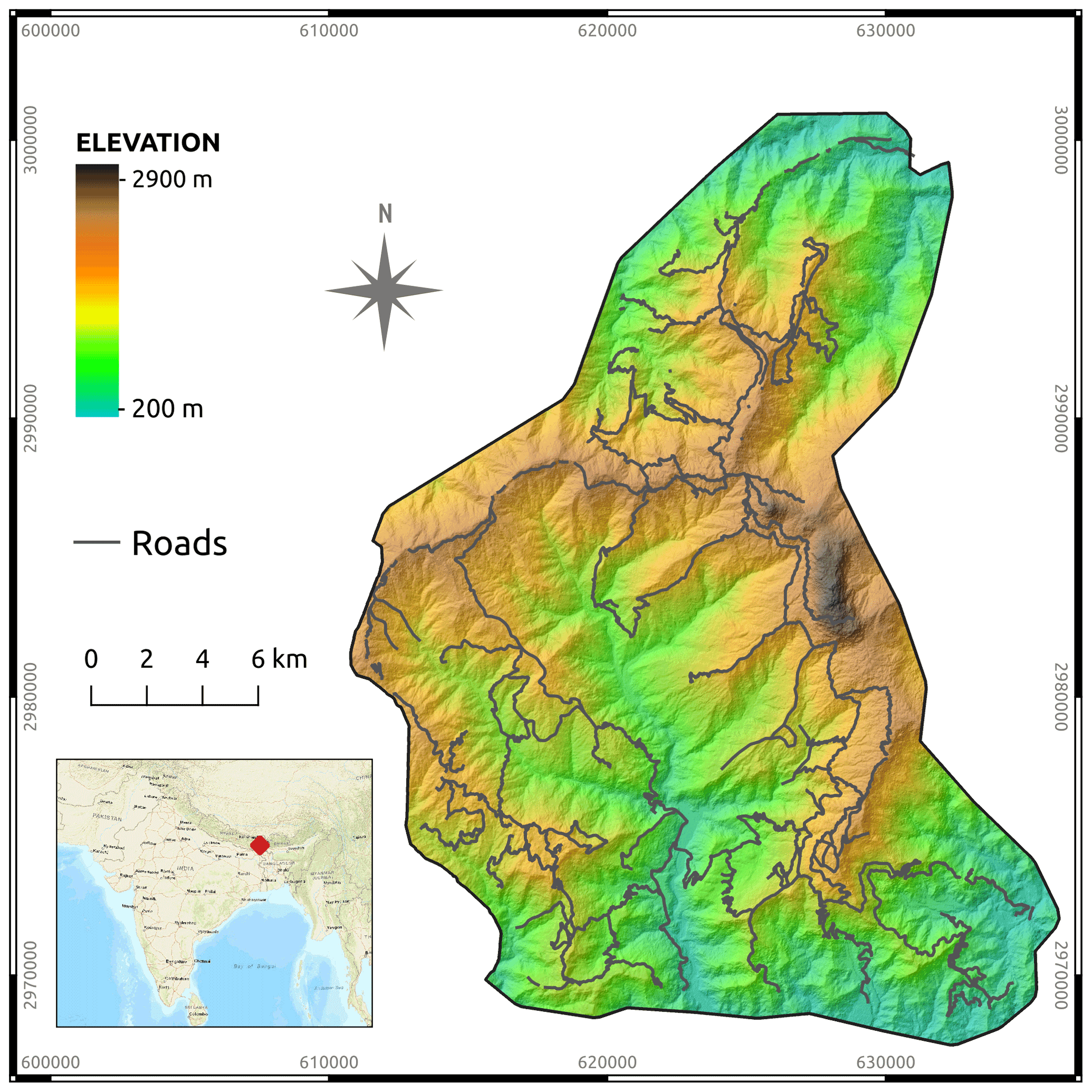
Figure 1Location map of the Darjeeling district (India). Projection: WGS 84/UTM zone 45N. Inset: location base map based on © OpenStreetMap contributors 2022. Distributed under the Open Data Commons Open Database License (ODbL) v1.0.
The Darjeeling study area experiences a temperate climate with wet summers which gradually moves into monsoon season when the area receives a number of wet spells, notorious for triggering landslides. This part of the eastern Himalayas receives the maximum amount of precipitation within the entire Himalayas.
The Darjeeling Himalayas is perennially landslide prone and frequently experiences landslide events of variable magnitudes. Most of these landslides are triggered by incessant monsoon rain between June and September, with some occasional major landsliding events in between. Notice that in Darjeeling roads are usually positioned along the relief's ridges (Fig. 1).
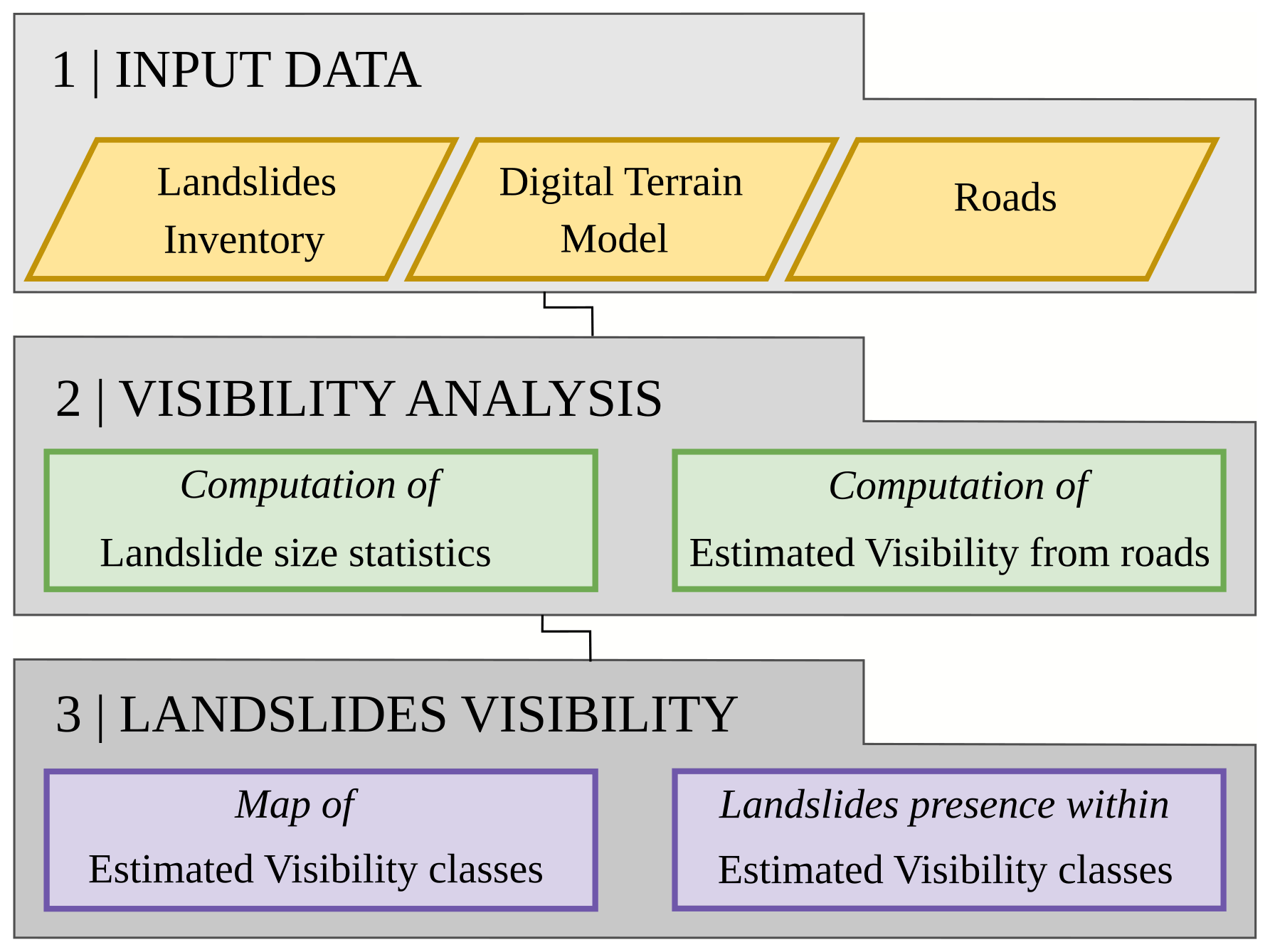
3.1 Methods
Estimated visibility (EV) simulates the visibility of an object from an observation point. In this paper EV is measured by the “solid angle” (SA; unit of measurement: square minutes [min2]), a metric that quantifies the level of visibility of an object, of known size and orientation, located at a certain distance from an observer or, in other words, a metric that measures the portion of the observer field of view occupied by an object.
We intend here the visibility of a landslide as the portion of the field of view of an observer occupied by the landslide itself, and we estimate it (estimated visibility, or EV) through the relative solid angle (SA) in square minutes. The apex is the point from which the slope is observed and the landslide subtends its solid angle from that point. The EV depends then from the size and the orientation of the slope/landslide, and the distance. (Fig. S1 in the Supplement illustrates the concept of EV and solid angle.)
We used r.survey to simulate the EV (Bornaetxea and Marchesini, 2021; Marchesini and Bornaetxea, 2022). The r.survey is an open source spatial analysis tool useful in assessing how the terrain morphology is perceived by an observer located at a defined observation point, or a group of points. It was designed for evaluating the visibility of features lying on the terrain slopes, including landslides. Among the different outputs, the tool provides the map of the maximum SA. In the maximum solid angle map, each pixel has only one value. However, each pixel is potentially observed from several observation points. Here, the pixel value represents the maximum solid angle value calculated among all observation points from which the pixel is visible. The SA value depends on the size of the observed object, the distance (between observers and target) and the relative orientation of the target with respect to the observation point.
The data required to run r.survey are a digital terrain model (DTM), a landslide inventory and a set of points of observations.
In this work, during the field surveys, the surveyors mainly travel on roads. Consequently, the simulation of visibility was performed starting from the road network. For this purpose, we generated a set of closely spaced points along the roads to simulate the observation points of a surveyor moving along the roads. Then we used r.survey to calculate the maximum SA map for a circular object, similar in size to the smallest landslide in the inventory. The SA values were then collapsed into SA classes in order to obtain an EV map. Additionally, we filtered the EV map by replacing the central pixel values with the most frequent class (mode) in a 3×3 moving window, in order to remove isolated pixels belonging to different classes with respect to the surrounding ones. Finally, we estimated the landslide density counting the number of landslides in each SA class. Since landslides are commonly collected as polygonal areas, it may happen that a single landslide overlaps more than one SA class. In this case, we assigned the landslide to the most present class within the landslide polygon.
We used two metrics to measure the spatial density: the normalised landslide count (NLC) and the standardised landslide density (SLD).
We used NLC to compare the spatial density of landslides included in different inventories prepared for the same study area (Eq. 1):
where ni and nt represent the number of landslides in the SA class i and the total number of landslides, in the inventory, respectively.
Alternatively, we used SLD (Eq. 2) to compare the spatial density of landslides inventories prepared for different study areas (see Sect. 4.3):
where Ai and At are respectively the area of SA class i and the total area.
The SLD metric normalises NLC according to the percentage of territory occupied by the SA classes. These percentages, in fact, can be slightly different among the study areas, due to the smoothing performed to remove isolated pixels.
The entire flowchart is shown in Fig. 2.
3.2 Data
The Geological Survey of India (GSI) provided us with an inventory that was the result of a fieldwork campaign carried out after the monsoon period (June–September) of 2019. This inventory, named GSI Field, provides landslide locations as points. Additionally, GSI also provided us with an historical landslide inventory (GSI Historic) for the Darjeeling area. It is a multi-temporal landslide inventory devoted to landslide susceptibility modelling and studying triggering mechanisms, landslide domains and mitigation actions. This database gathers information about landslides that have occurred since 1968. As usually occurs with national or regional multi-temporal databases (van Den Eeckhaut and Hervás, 2012), the information in this database is heterogeneous. Out of 1240 landslides, 80 % are represented as polygons, while 20 % are single points. Almost half of the landslides (47.6 %) were mapped by means of satellite image photo interpretation, using the available images coming from diverse sources such as Cartosat PAN (2 %) (2.5 m × 2.5 m), LISS IV (1 %) (5.8 m × 5.8 m) and Google Earth, or other base satellite maps available in ESRI's ArcGIS 10.2 (44.6 %). The rest of the data came mainly from legacy data, including data collected from GSI reports, and Toposheet (34.6 %). The latter corresponds to a Topobase map of the Survey of India (SOI) surveyed in 1969–1970 at 1:25 000 scale. Other sources, such as the Darjeeling Himalayan Railway's database (7.5 %), blogs or newspapers (3.5 %) and fieldwork (6.8 %), complete the available information. Debris slides (69.43 %) and rock slides (18.4 %) are the most frequently reported failures together with debris flows (5.3 %), rock fall (0.23 %), deep rotational slides (1.95 %) and unknown causes (4.69 %). Lastly, we mapped landslides triggered by the 2019–2020 monsoon season using a pre-event pan sharpened Spot 6 image acquired on 22 March 2019 and a pan sharpened post-event image acquired on 3 April 2020 by the same satellite. We used the two 2.5 × 2.5 m spatial resolution images to detect landslides occurring in between the two acquisitions following a photo-interpretation approach. In this inventory, referred to as Spot 2020, we classified most of the landslides (95 %) as earth and debris flows, and the rest as complex movements. Figure 3 shows that GSI Historic and Spot 2020 FAD curves reveal a power law shape on the right of the rollover value (Malamud et al., 2004). The FAD curve could not be computed for GSI Field inventory due to the absence of the information about the landslide sizes. Figure 3 also describes some characteristics of the available inventories.

Figure 3Frequency area distribution curves (FAD curves) for Spot 2020 (green) and GSI Historic (brown). Landslide distribution map for Spot 2020, GSI Historic and GSI Field. Summary table of the inventories.
In addition to the landslide information, GSI also provided us with the road network map of Darjeeling, together with the 10 × 10 m resolution DTM.
4.1 Classified estimated visibility map
We obtained the EV map of the study area using r.survey with the settings listed in Table 1. We used the entire road network (including roads slightly outside the boundaries of the studied area) and a maximum distance between points of 50 m for modelling the estimated visibility of an observer moving along the study area. We considered all the possible roads accessible in the study area, even though this probably overestimates the actual places from which the territory is commonly observed.
The EV map was calculated for hypothetical landslides with an area equal to 78.54 m2, which corresponds to the smallest landslides inventoried in Darjeeling (Table 1). We set to infinity the maximum line of sight distance in order to assess the visibility level for the complete territory.
Table 1Summary of the specific settings to calculate SA maps for each study area.

We classified the EV map into six classes using the 16.67th, 33.33rd, 50th, 66.67th, 83.33rd and 100th quantiles of the SA map values as thresholds. Then we applied a 3 × 3 smoothing moving window. Details about the threshold values for each SA class are available in Fig. 4.
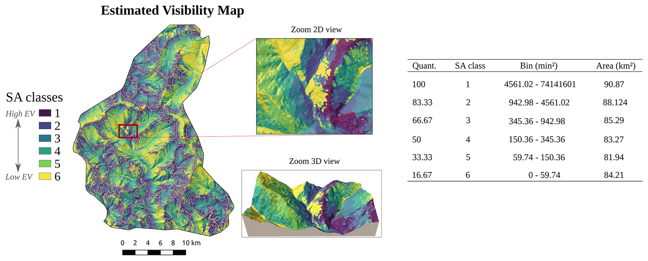
Figure 4EV map for an object having a size of 78.54 m2. Red lines in the zoom insets represent the roads used as reference observation points. The abbreviation Quant. refers to quantiles and min2 stands for square minutes, a unit of measure of the solid angle.
We carried out a spatial analysis to investigate possible natural causes for different landslide densities in the different SA classes. Terrain slope, lithology and land use are the most important factors that may condition the occurrence of landslides (Reichenbach et al. 2018). So, we analysed the empirical densities distribution of the slope values and the percentual spatial coverage of the lithology and land cover categories inside each SA class. Figure 5 shows that slope empirical distributions are similar among the SA classes, and so are the distributions of the lithological and land cover categories. Data in Fig. 5 suggest that any difference in landslide density, between SA classes, is unlikely to be related to morphology, land cover and lithology.
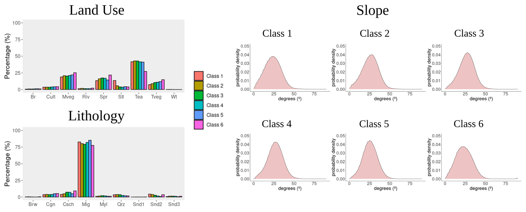
Figure 5Slope probability density plots and land use and lithology distribution by SA classes for Darjeeling study areas. Land use types are Br: barren; Cult: cultivated land; Mveg: moderate vegetation; Riv: river; Spr: sparse vegetation; Stl: settlement; Tea: tea plantation; Tveg: thick vegetation; Wt: water body. The lithology types are Brw: brownish, yellow oxidised soil with boulders or pebbles and latsol; Cgn: calc granulite, quartzite, gneiss, gar, sil, kya schists; Csch: chlorite sericite schist and quartzite, metagraywacke; Mig: banded migmatite, Gt–Bt gneiss, mica schist, biotite gneiss; Myl: mylonitic granite gneiss; Qrz: quartz arenite, black slate, cherty phyllite, quartzite; Snd1: sand, silt and clay; Snd2: sandstone, clay, shale, conglomerate; Snd3: sandstone, shale with minor coal.
4.2 Description and analysis of NLC plots
Figure 6 shows NLC versus the SA classes of the EV map, for the available landslide inventories. Figure 6a shows that, in the GSI Field inventory (a field-based inventory), most of the landslides are located within the classes having higher SA values (class 1 and class 2). Landslide density in the other classes is very fluctuating, probably due to the small number of landslides in the inventory.
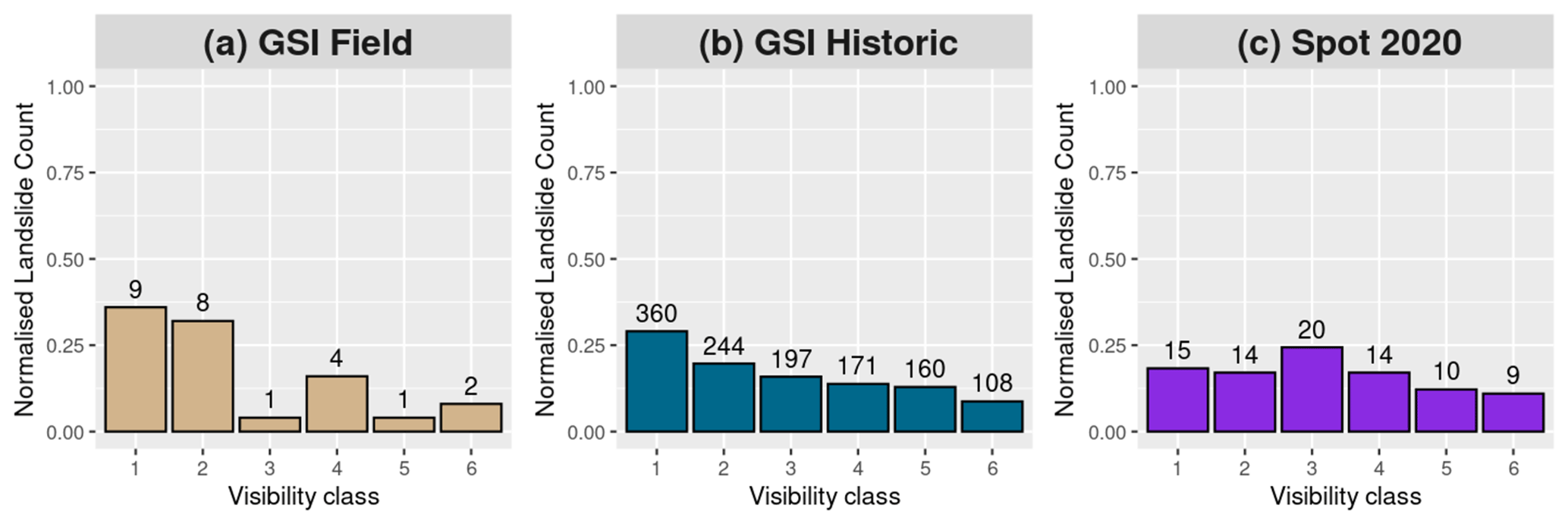
Figure 6Normalised landslide count plot for GSI Field, GSI Historic and Spot 2020 inventories. The values above each column signify the number of landslides in each SA class.
GSI Historic (Fig. 6b) includes landslides mapped using different methods. It shows a slight, but monotonic, decreasing trend.
Figure 6c shows the calculated NLC values for the Spot 2020 inventory, produced through photo interpretation of satellite imagery. The values calculated in the SA classes are fairly homogeneous and without trends.
The GSI Historic inventory contains two main types of information: landslides mapped exploiting satellite/aerial images or collected during field-based survey and from legacy data. We separated data obtained by satellite/aerial images from the rest of the data sources and called them GSI Historic Sat and GSI Historic Others respectively.
The NLC values show a pronounced monotonic decreasing trend for the GSI Historic Others inventory (Fig. 7a), while GSI Historic Sat (Fig. 7b) behaves similarly to the Spot 2020 inventory (Fig. 6c), with the landslide density not dependent on SA classes.
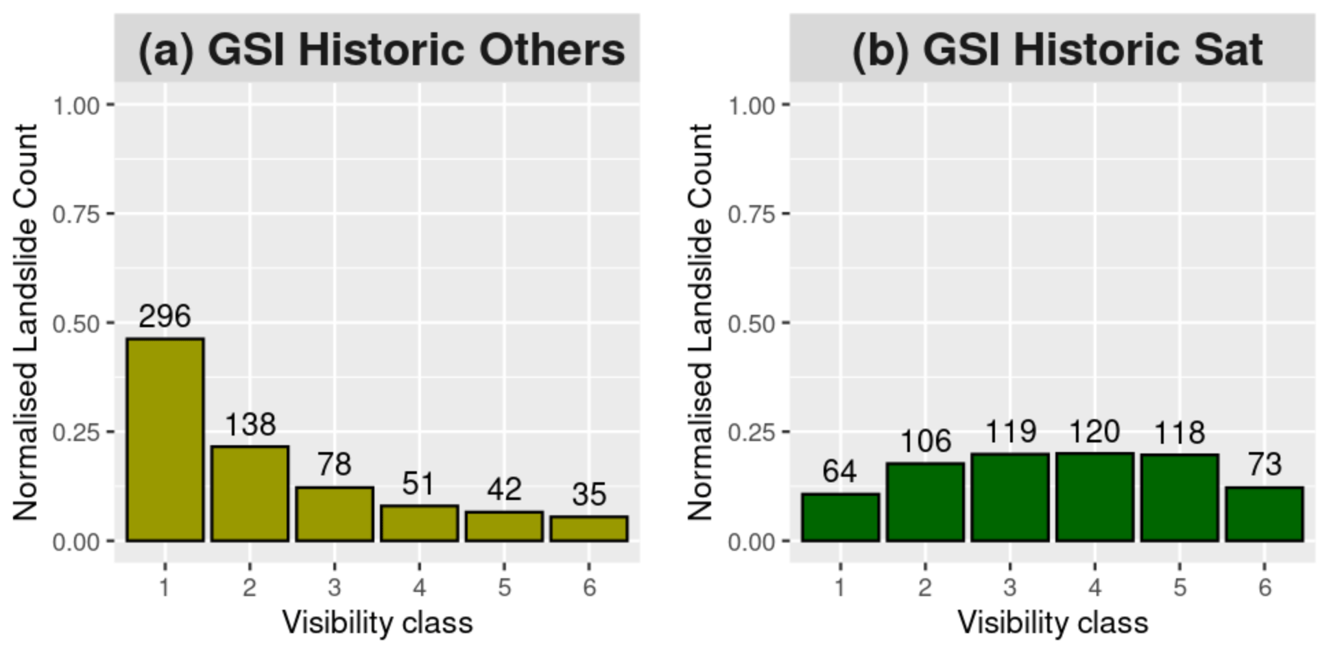
Figure 7Normalised landslide count distribution plot for GSI Historic Others and GSI Historic Sat inventories. The values above each column signify the absolute number of landslides in each visibility class.
We additionally compared landslide sizes in the different SA classes (Fig. 8). In GSI Historic Others we merged classes 4–6 to have enough samples. We did not consider Spot 2020 and GSI Field inventories because of the little amount of data.
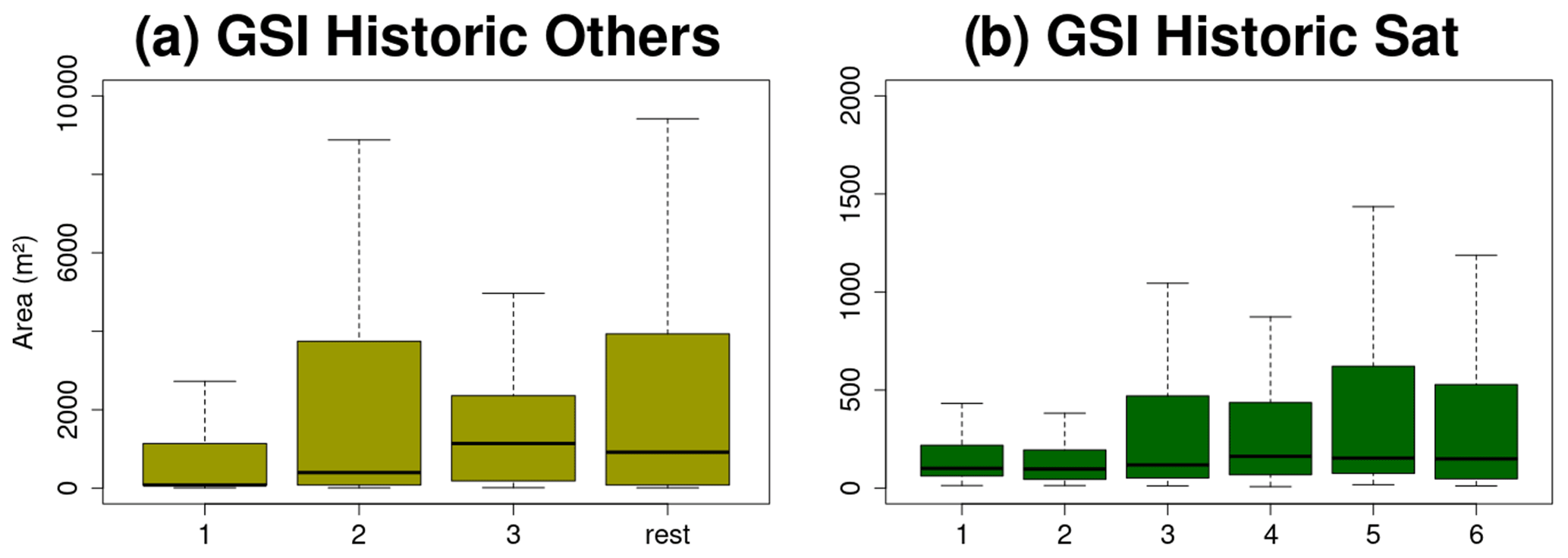
Figure 8Landslide area boxplots per SA classes. Numbers on the x axis are the SA classes of the EV map. The horizontal solid line inside each box indicates the median value.
Landslides in class 1 are significantly smaller than those included in the other classes for GSI Historic Others inventory (Fig. 8a). Furthermore, the landslide size median in this inventory tends to increase when the estimated visibility decreases (i.e. the median of the landslide area in classes 3–6 is up to 20 times larger than in classes 1 and 2). For the GSI Historic Sat we did not observe a clear increasing trend in the medians of the landslide sizes (Fig. 8b) which are more homogeneous across the SA classes (even if in classes 1 and 2 landslides are generally small).
4.3 Testing the method with external and modelled data
We performed two additional analyses to further confirm the observed behaviour. First, we verified how many of the landslides recorded in Spot 2020 and GSI Historic Sat inventories would have been visible if observed from the same roads used to estimate the visibility for the other inventories. Second, we applied the EV analysis to a purely field-based inventory available for a different study area.
For the first analysis we estimated the solid angle of the landslides included in Spot 2020 and GSI Historic Sat inventories (by considering their real size). Then we selected only those landslides with an SA larger than 400 min2, which is a value slightly larger than a person's maximum visual acuity (Bornaetxea and Marchesini, 2021; Healey and Sawant, 2012). We refer to these two samples as “Spot 2020 visible” and “GSI Historic Sat visible” respectively. In this scenario, the number of (potentially) visible landslides became 55 for “Spot 2020 visible” and 301 for “GSI Historic Sat visible”, i.e. −59.8 % and −32.9 % with respect to the original data sets.
For the second analysis we used a landslide inventory prepared, by one of the authors, during a field-work campaign carried out in the period from June to August 2016 in Gipuzkoa Province (Spain) (Bornaetxea et al., 2018). We decided to run an extra experiment with this data set because we sought confirmation of the relevant role played by EV in influencing the spatial distribution of landslides in the inventories. In fact, since in Gipuzkoa information on the detailed road route followed by the surveyor was available, we expected the distribution of landslides to be even more influenced by visibility than in Darjeeling, where, due to the absence of specific information, the simulation of visibility was done using the entire road network. This additional inventory includes 542 shallow landslides and is referred to as Gipuzkoa inventory. We applied the approach explained in Sect. 3 but using a 5 × 5 m resolution DTM and a distance of 200 m between observation points. (Figure S2 in the Supplement shows the EV map obtained from the visibility analysis in Gipuzkoa.)
Results are shown in Fig. 9, where we compared the standardised landslide density (SLD; see Sect. 3) values with respect to the central value of each SA class. The SA values are plotted in logarithmic scale and we excluded GSI Field and GSI Historic inventories from this analysis due to data scarcity or because of the non-homogeneous source of the data.
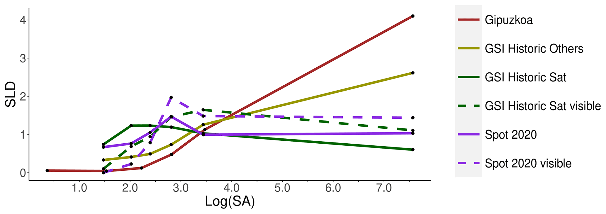
Figure 9Standardised landslide density plot for six different landslide inventories. Spot 2020 visible and GSI Historic Sat visible are simulated sub-samples of Spot 2020 and GSI Historic Sat respectively.
In Fig. 9 we observe that, for values of log(SA) smaller than about 3.0 (where the central value of the SA classes 3–6 are), “Spot 2020 visible” and “GSI Historic Sat visible” show a marked reduction in the SLD with respect to the original Spot 2020 and GSI Historic Sat inventories. The reduction is caused by the worse visibility from roads than from satellites in classes 3–6.
In the same range of log(SA) values, the pattern of SLD for the “Spot 2020 visible” and “GSI Historic Sat visible” inventories is monotonically non-decreasing, likewise the GSI Historic Others inventory.
From Fig. 9 we note that also the Gipuzkoa inventory, entirely field based, shows a marked monotonically non-decreasing pattern. The SLD curve is similar to GSI Historic Others in shape, which suggests that both show a substantial dependence on the EV. This is also conformal to the pattern of the SLD values for the “Spot 2020 visible” and “GSI Historic Sat visible” inventories when SA is low. In contrast, GSI Historic Sat and Spot 2020 show an almost flat behaviour, where the number of landslides does not vary according to the EV from the roads.
It is interesting to note that for the highest log(SA) values (i.e. for estimated visibility class 1), the SLD values for “Spot 2020 visible” and “GSI Historic Sat visible” are similar to those in the original inventories. This shows that the landslides in class 1 can all be mapped from roads.
In this paper we assess the CoLM uniformity of landslide inventories in relation to the visibility offered by well-known observation points. We estimated the visibility offered by a set of points of observation using a geometric approach that takes into account the local morphology of a territory. The most visible areas are generally located near the points of observations (i.e. roads in this work). But unlike in the geometric distance buffering, the SA classes show a non-symmetrical propagation of the EV, which allows detection of portions of territories very close to roads but poorly visible (Fig. 4).
The spatial densities of landslide information (measured by the NLC and SLD metrics) and the EV are positively related to the GSI Field (Fig. 6a) and GSI Historic Others (Fig. 7a) inventories. The deviations from a monotonic trend, observed in the GSI Field inventory, are probably related to the low data density and location inaccuracy. Since the distribution of the main landslide predisposing factors is homogeneous across all the SA classes (Fig. 5), we consider these trends as relevant evidence of the scarce CoLM uniformity of the inventories and, as a consequence, of their uneven completeness. On the contrary, for the satellite imagery-based inventories (Spot 2020 and GSI Historic Sat) the NLC and SLD values in the SA classes are quite uniform (Figs. 6c and 7b). This is assumed to be a consequence of the neutral CoLM uniformity offered by the remote acquisition.
Roads, which are by definition always included in the first visibility class, are also considered by many authors as a predisposing factor since cut-and-fill failures, drainage and groundwater alteration can influence the occurrence of landslides (Brenning et al., 2015; Donnini et al., 2017; Giordan et al., 2018; McAdoo et al., 2018). Moreover, Taylor et al. (2020) suggest that transport networks and landslides are interconnected in terms of process and impacts. Indeed, Tanyaş et al. (2022) also state that road construction acts as a major causative factor of landslides. However, the reasons of that close relationship are very complex and not fully unravelled (Meneses et al., 2019; Santangelo et al., 2015; Sidle et al., 2014; Sidle and Ziegler, 2012), which justifies the need to investigate whether the major availability of roadside landslide information in inventories may also depend on other factors.
Based on the above considerations, a higher density of landslides (higher NLC and SLD values) should be expected only along the roads and, as a consequence, in the SA class 1 with respect to the SA classes 2–6. But at the same time, all the SA classes, except for the first one, should show fairly similar density of landslides. In inventories based on satellite imagery (GSI Historic Sat and Spot 2020) the latter condition was fulfilled, but we did not observe a higher number of landslides in SA class 1 (Figs. 6c and 7b). In the GSI Field and GSI Historic Others, the abundance in SA class 1 is evident, but the number of landslides still drops monotonically also in SA classes 2–6. So, we conclude that in both types of inventories, there is a data collection effect (Steger et al., 2021), albeit different.
In fact, since roadside landslides are typically small (Voumard et al., 2018), they can be easily under-represented when the inventories are prepared with images without an adequate resolution or unsuitable acquisition geometry (Martha et al., 2021). When considering GSI Historic Others, landslides are very abundant in the highly visible areas (Fig. 7a), and at the same time they are considerably smaller than in the rest of the classes (Fig. 8a). On the contrary, for GSI Historic Sat inventory, comparing Figs. 7b and 8b, we observe a relatively low number of small size landslides in class 1. In this case, limits in the type and quality of the satellite images (e.g. spatial resolution, acquisition time and geometry, etc.) can be the factors hampering the possibility of mapping small landslides (Mondini et al., 2014). Furthermore, in GSI Historic Sat the variation of landslide size in the different visibility classes does not show a clear trend and presents much smaller variations than in GSI Historic Others inventories (Fig. 8), where the size of the mapped landslides rises progressively according to the lack of visibility. This suggests that the visibility can also affect the size distributions (Fig. 8) of the reported landslide information. These results are in line with the Steger et al. (2021) hypothesis on the “data collection effect”, which states that the method used to compile inventories can influence the distribution of landslide information in the inventories.
We observed a partially monotonic behaviour in the relationship between estimated visibility and landslide density obtained in the field and historic-based inventories also in Spot 2020 Visible and GSI Historic Sat Visible. These two inventories include only those landslides present in the remotely sensed inventories that would result as visible through hypothetical field surveys along the roads. The SLD values (Fig. 9) highlight that the least visible areas (low SA values) lost the majority of landslides. Moreover, in the most visible areas, SLD values from the Spot 2020 Visible and GSI Historic Sat Visible inventories are much lower than those observed for the GSI Historic Others. This possibly suggests that some small landslides were not detected in visibility class 1 for Spot 2020 and GSI Historic Sat, eventually caused by the inadequate resolution of the images. We conclude that even if the CoLM uniformity of the landslide inventories produced using satellite-based images is generally large, they can still be unable to reach, in the SA class 1 (i.e. in the areas very visible from the roads), the same completeness they have in the other SA classes.
The monotonic non-decreasing trend observed for field-based or legacy-based landslide inventories was confirmed by the analysis carried out with a landslide inventory prepared in a completely different study area, in Spain (Gipuzkoa). For this inventory, the accurate road path followed by the surveyor was also well known and there was not the need to conservatively assess the EV along the entire road network (as we did for the Darjeeling study area). This allowed a more accurate simulation of the EV which, in turn, determined a pronounced non-descending monotonic pattern of the SLD values (Fig. 9). Results obtained on Gipuzkoa confirm that by means of the EV analysis it is possible to assess the CoLM uniformity of an inventory, and therefore also of its completeness. In addition, the use of the SLD metric makes it possible to compare the CoLM uniformity of different inventories produced in the same or in different study areas.
Notwithstanding these observations, we acknowledge that our results depend on some user-driven decisions, such as the distance between observation points placed along the roads, and the choice of the thresholds to obtain the visibility classes. In Darjeeling, the real path followed by the field surveyor was unknown and we applied a conservative approach (visibility overestimation) by considering all roads as potential observation points and a four-times-smaller maximum distance between points than in Gipuzkoa. This is probably one of the reasons for the more pronounced monotonic pattern shown in Gipuzkoa with respect to GSI Historic Others. Furthermore, we chose quantile values of the EV map to obtain the SA classes covering similar portions of the study area. We run several tests with different threshold values showing results in terms of landslide densities always very similar to those described by Figs. 6, 7, and 9.
The resolution of the DTM can also have an impact on the results. A coarse representation of the morphology of the territory can affect the calculation of the solid angle and the delineation of non-visible areas. In this work, we performed the analysis with the higher resolution DTMs available in each study area, but further tests on the influence of the quality of the data should be conducted. Future works should also incorporate the role of the vegetation in the visibility for landslide detection by fieldwork, although the information about the elevation of each type of vegetation is rare.
In addition, although EV could be measured using different metrics (e.g. by counting the number of points that have a direct line of sight to a particular object (Fontani, 2017), we maintain that our method offers the unique perspective of considering several geometric aspects of the object and the territory under investigation. This makes our approach appropriate for morphologically complex areas.
We analysed the relationship between the spatial density of landslides reported in different inventories prepared through field surveys, collection of previous data and interpretation of remotely acquired images, and the visibility of the territory from observation points located along the roads. We also introduced the concept of uniformity in capacity of landslide mapping (CoLM) as a tool to discern whether the completeness of a landslide inventory is homogeneous across the territory.
The results of the present work show that in inventories prepared using field survey and/or historic legacy data, the CoLM uniformity can be poor, and this is reflected in marked inhomogeneity in completeness. This is demonstrated by (i) the positive correlation observed between landslide density and the visibility of the terrain from the observation points, (ii) the lack of small landslides in areas with low visibility and (iii) a number of landslides in remote areas intercepted by the satellite images but invisible from roads.
In addition, we observed that inventories based on the use of remote sensing images, where the CoLM is uniform, may also be affected by a different form of “data collection effect” (sensu Steger et al., 2021). In fact, results show that, contrary to what is expected (Brenning et al., 2015; Donnini et al., 2017; Giordan et al., 2018; McAdoo et al., 2018; Meneses et al., 2019; Santangelo et al., 2015; Sidle et al., 2014; Sidle and Ziegler, 2012), our inventories do not show an abundance of landslides close to roads. The reasons may be due to the inadequate spatial resolution of the satellite images, which can prevent the recognition of small roadside landslides. Thus, our inventories proved not to be uniformly representative of the real spatial distribution of landslides in the study area, requiring an informed and appropriate usage (Bornaetxea et al., 2018; Steger et al., 2021).
Our procedure enriches the portfolio of solutions to evaluate the quality of landslide inventories introducing local morphology in the analysis. We think that the procedure and methods presented in this work can be used in other study areas to: (i) test whether the information in existing inventories (especially those created by fieldwork) is affected by a scarce CoLM (and therefore completeness) uniformity, (ii) identify portions of land where landslide density information is larger with respect to other areas and can be more properly used to train susceptibility, hazard and risk models, (iii) identify portions of land where landslide inventories need improvement and (iv) plan exhaustive field mapping campaigns.
The digital elevation model of Gipuzkoa Province with 5 × 5 m of resolution was downloaded from the official geospatial data repository https://www.geo.euskadi.eus/modelo-digital-del-terreno-mdt-remuestreado-de-5m-de-la-comunidad-autonoma-del-pais-vasco-ano-2016/webgeo00-dataset/es/ (Govierno Vasco, 2016). The Gipuzkoa inventory and the field work paths are data generated by the authors and are available upon request. The digital elevation model of Darjeeling with 10 × 10 m resolution road maps of Darjeeling and all the landslide inventories used in this work were provided by the Geological Survey of India. The tool r.survey is available at https://doi.org/10.5281/zenodo.3993140 (Marchesini and Bornaetxea, 2022).
The supplement related to this article is available online at: https://doi.org/10.5194/nhess-22-2929-2022-supplement.
TB and IM conceptualised the work and designed the overall methodology. TB carried out the analysis with the technical assistance of IM and AM. SK and RK provided the necessary data and contributed to the interpretation of the results through their local perspective. TB prepared the first version of the manuscript, and IM and AM contributed enormously to its revision. AM coordinated the work and obtained the necessary funds.
The contact author has declared that none of the authors has any competing interests.
Publisher’s note: Copernicus Publications remains neutral with regard to jurisdictional claims in published maps and institutional affiliations.
The work was partially funded by the UKRI Natural Environment Research Council's and UK Government's Department for International Development's Science for Humanitarian Emergencies and Resilience research programme. Txomin Bornaetxea was financially supported by the postdoctoral fellowship program of the Basque government in the framework of a scientific collaboration with the Geological Survey of Canada and during the scientific collaborations with the Geomorphological Group of the Research Institute for the Geo-Hydrological Protection in Perugia, Italian National Research Council (CNR-IRPI).
This research has been supported by the Natural Environment Research Council (grant no. NERC/DFID NE/P000649/1) and the Eusko Jaurlaritza (grant no. POS_2020_2_0010).
This paper was edited by Andreas Günther and reviewed by Elena Petrova and two anonymous referees.
Bera, S., Guru, B., and Ramesh, V.: Evaluation of landslide susceptibility models: A comparative study on the part of Western Ghat Region, India, Remote Sens. Appl. Soc. Environ., 13, 39–52, https://doi.org/10.1016/j.rsase.2018.10.010, 2019.
Bornaetxea, T. and Marchesini, I.: r.survey: a tool for calculating visibility of variable-size objects based on orientation, Int. J. Geogr. Inf. Sci., 36, 429–452, https://doi.org/10.1080/13658816.2021.1942476, 2021.
Bornaetxea, T., Rossi, M., Marchesini, I., and Alvioli, M.: Effective surveyed area and its role in statistical landslide susceptibility assessments, Nat. Hazards Earth Syst. Sci., 18, 2455–2469, https://doi.org/10.5194/nhess-18-2455-2018, 2018.
Brenning, A., Schwinn, M., Ruiz-Páez, A. P., and Muenchow, J.: Landslide susceptibility near highways is increased by 1 order of magnitude in the Andes of southern Ecuador, Loja province, Nat. Hazards Earth Syst. Sci., 15, 45–57, https://doi.org/10.5194/nhess-15-45-2015, 2015.
Cascini, L.: Applicability of landslide susceptibility and hazard zoning at different scales, Eng. Geol., 102, 164–177, https://doi.org/10.1016/j.enggeo.2008.03.016, 2008.
Chaparro-Cordón, J. L., Rodríguez-Castiblanco, E .A., Rangel-Flórez, M. S., García-Delgado, H., and Medina-Bello, E.: Statistical description of some landslide inventories from Colombian Andes: study cases in Mocoa, Villavicencio, Popayán, and Cajamarca, SCG-XIII International Symposium on Landslides 2020, Cartajena, Colombia, 15–19 June 2020, https://doi.org/10.13140/RG.2.2.17237.04327, 2020.
Corominas, J., van Westen, C., Frattini, P., Cascini, L., Malet, J.-P., Fotopoulou, S., Catani, F., van Den Eeckhaut, M., Mavrouli, O., Agliardi, F., Pitilakis, K., Winter, M. G., Pastor, M., Ferlisi, S., Tofani, V., Hervás, J., and Smith, J. T.: Recommendations for the quantitative analysis of landslide risk, B. Eng. Geol. Environ., 73, 209–263, https://doi.org/10.1007/s10064-013-0538-8, 2014.
Domingo-Santos, J. M., de Villarán, R. F., Rapp-Arrarás, Í., and de Provens, E. C.-P.: The visual exposure in forest and rural landscapes: An algorithm and a GIS tool, Landscape Urban Plan., 101, 52–58, https://doi.org/10.1016/j.landurbplan.2010.11.018, 2011.
Donnini, M., Napolitano, E., Salvati, P., Ardizzone, F., Bucci, F., Fiorucci, F., Santangelo, M., Cardinali, M., and Guzzetti, F.: Impact of event landslides on road networks: a statistical analysis of two Italian case studies, Landslides, 14, 1521–1535, https://doi.org/10.1007/s10346-017-0829-4, 2017.
Fell, R., Corominas, J., Bonnard, C., Cascini, L., Leroi, E., and Savage, W. Z.: Guidelines for landslide susceptibility, hazard and risk zoning for land-use planning, Eng. Geol., 102, 99–111, https://doi.org/10.1016/j.enggeo.2008.03.014, 2008.
Fiorucci, F., Giordan, D., Santangelo, M., Dutto, F., Rossi, M., and Guzzetti, F.: Criteria for the optimal selection of remote sensing optical images to map event landslides, Nat. Hazards Earth Syst. Sci., 18, 405–417, https://doi.org/10.5194/nhess-18-405-2018, 2018.
Fontani, F.: Application of the Fisher's “Horizon Viewshed” to a proposed power transmission line in Nozzano (Italy), T. GIS, 21, 835–843, https://doi.org/10.1111/tgis.12260, 2017.
Fressard, M., Thiery, Y., and Maquaire, O.: Which data for quantitative landslide susceptibility mapping at operational scale? Case study of the Pays d'Auge plateau hillslopes (Normandy, France), Nat. Hazards Earth Syst. Sci., 14, 569–588, https://doi.org/10.5194/nhess-14-569-2014, 2014.
Galli, M., Ardizzone, F., Cardinali, M., Guzzetti, F., and Reichenbach, P.: Comparing landslide inventory maps, Geomorphology, 94, 268–289, https://doi.org/10.1016/j.geomorph.2006.09.023, 2008.
Gariano, S. L. and Guzzetti, F.: Landslides in a changing climate, Earth-Sci. Rev., 162, 227–252, https://doi.org/10.1016/j.earscirev.2016.08.011, 2016.
Ghorbanzadeh, O., Meena, S. R., Blaschke, T., and Aryal, J.: UAV-Based Slope Failure Detection Using Deep-Learning Convolutional Neural Networks, Remote Sens., 11, 2046, https://doi.org/10.3390/rs11172046, 2019.
Giordan, D., Hayakawa, Y., Nex, F., Remondino, F., and Tarolli, P.: Review article: the use of remotely piloted aircraft systems (RPASs) for natural hazards monitoring and management, Nat. Hazards Earth Syst. Sci., 18, 1079–1096, https://doi.org/10.5194/nhess-18-1079-2018, 2018.
Govierno Vasco: Modelo Digital del Terreno (MDT) remuestreado de 5 m de la Comunidad Autónoma del País Vasco, Año 2016, GEOEUSKADI [data set], https://www.geo.euskadi.eus/modelo-digital-del-terreno-mdt-remuestreado-de-5m-de-la-comunidad-autonoma-del-pais-vasco-ano-2016/webgeo00-dataset/es/ (last access: May 2020), 2016.
Guzzetti, F., Carrara, A., Cardinali, M., and Reichenbach, P.: Landslide hazard evaluation: a review of current techniques and their application in a multi-scale study, Central Italy, Geomorphology, 31, 181–216, https://doi.org/10.1016/S0169-555X(99)00078-1, 1999.
Guzzetti, F., Reichenbach, P., Ardizzone, F., Cardinali, M., and Galli, M.: Estimating the quality of landslide susceptibility models, Geomorphology, 81, 166–184, https://doi.org/10.1016/j.geomorph.2006.04.007, 2006.
Guzzetti, F., Mondini, A. C., Cardinali, M., Fiorucci, F., Santangelo, M., and Chang, K.-T.: Landslide inventory maps: New tools for an old problem, Earth-Sci. Rev., 112, 42–66, https://doi.org/10.1016/j.earscirev.2012.02.001, 2012.
Hao, L., Rajaneesh A., van Westen, C., Sajinkumar K. S., Martha, T. R., Jaiswal, P., and McAdoo, B. G.: Constructing a complete landslide inventory dataset for the 2018 monsoon disaster in Kerala, India, for land use change analysis, Earth Syst. Sci. Data, 12, 2899–2918, https://doi.org/10.5194/essd-12-2899-2020, 2020.
Healey, C. G. and Sawant, A. P.: On the limits of resolution and visual angle in visualization, ACM T. Appl. Percept., 9, 1–21, https://doi.org/10.1145/2355598.2355603, 2012.
Hussain, G., Singh, Y., Singh, K., and Bhat, G. M.: Landslide susceptibility mapping along national highway-1 in Jammu and Kashmir State (India), Innov. Infrastruct. Solut., 4, 59, https://doi.org/10.1007/s41062-019-0245-9, 2019.
Jacobs, L., Kervyn, M., Reichenbach, P., Rossi, M., Marchesini, I., Alvioli, M., and Dewitte, O.: Regional susceptibility assessments with heterogeneous landslide information: Slope unit- vs. pixel-based approach, Geomorphology, 356, 107084, https://doi.org/10.1016/j.geomorph.2020.107084, 2020.
Knevels, R., Petschko, H., Proske, H., Leopold, P., Maraun, D., and Brenning, A.: Event-Based Landslide Modeling in the Styrian Basin, Austria: Accounting for Time-Varying Rainfall and Land Cover, Geosciences, 10, 217, https://doi.org/10.3390/geosciences10060217, 2020.
Lee, S., Jang, J., Kim, Y., Cho, N., and Lee, M.-J.: Susceptibility Analysis of the Mt. Umyeon Landslide Area Using a Physical Slope Model and Probabilistic Method, Remote Sens., 12, 2663, https://doi.org/10.3390/rs12162663, 2020.
Lima, P., Steger, S., and Glade, T.: Counteracting flawed landslide data in statistically based landslide susceptibility modelling for very large areas: a national-scale assessment for Austria, Landslides, 18, 3531–3546, https://doi.org/10.1007/s10346-021-01693-7, 2021.
Malamud, B. D., Turcotte, D. L., Guzzetti, F., and Reichenbach, P.: Landslide inventories and their statistical properties, Earth Surf. Proc. Land., 29, 687–711, https://doi.org/10.1002/esp.1064, 2004.
Marchesini, I. and Bornaetxea, T.: r.survey.py, Zenodo [code], https://doi.org/10.5281/zenodo.3993140, 2022.
Martha, T. R., Roy, P., Jain, N., Khanna, K., Mrinalni, K., Kumar, K. V., and Rao, P. V. N.: Geospatial landslide inventory of India – an insight into occurrence and exposure on a national scale, Landslides, 18, 2125–2141, https://doi.org/10.1007/s10346-021-01645-1, 2021.
McAdoo, B. G., Quak, M., Gnyawali, K. R., Adhikari, B. R., Devkota, S., Rajbhandari, P. L., and Sudmeier-Rieux, K.: Roads and landslides in Nepal: how development affects environmental risk, Nat. Hazards Earth Syst. Sci., 18, 3203–3210, https://doi.org/10.5194/nhess-18-3203-2018, 2018.
Meena, S. R., Mishra, B. K., and Tavakkoli Piralilou, S.: A Hybrid Spatial Multi-Criteria Evaluation Method for Mapping Landslide Susceptible Areas in Kullu Valley, Himalayas, Geosciences, 9, 156, https://doi.org/10.3390/geosciences9040156, 2019.
Melzner, S., Rossi, M., and Guzzetti, F.: Impact of mapping strategies on rockfall frequency-size distributions, Eng. Geol., 272, 105639, https://doi.org/10.1016/j.enggeo.2020.105639, 2020.
Meneses, B. M., Pereira, S., and Reis, E.: Effects of different land use and land cover data on the landslide susceptibility zonation of road networks, Nat. Hazards Earth Syst. Sci., 19, 471–487, https://doi.org/10.5194/nhess-19-471-2019, 2019.
Mondini, A. C., Viero, A., Cavalli, M., Marchi, L., Herrera, G., and Guzzetti, F.: Comparison of event landslide inventories: the Pogliaschina catchment test case, Italy, Nat. Hazards Earth Syst. Sci., 14, 1749–1759, https://doi.org/10.5194/nhess-14-1749-2014, 2014.
Nicu, I. C., Lombardo, L., and Rubensdotter, L.: Preliminary assessment of thaw slump hazard to Arctic cultural heritage in Nordenskiöld Land, Svalbard, Landslides, 18, 2935–2947, https://doi.org/10.1007/s10346-021-01684-8, 2021.
Park, J.-Y., Lee, S.-R., Lee, D.-H., Kim, Y.-T., and Lee, J.-S.: A regional-scale landslide early warning methodology applying statistical and physically based approaches in sequence, Eng. Geol., 260, 105193, https://doi.org/10.1016/j.enggeo.2019.105193, 2019.
Piacentini, D., Troiani, F., Daniele, G., and Pizziolo, M.: Historical geospatial database for landslide analysis: the Catalogue of Landslide OCcurrences in the Emilia-Romagna Region (CLOCkER), Landslides, 15, 811–822, https://doi.org/10.1007/s10346-018-0962-8, 2018.
Reichenbach, P., Rossi, M., Malamud, B. D., Mihir, M., and Guzzetti, F.: A review of statistically-based landslide susceptibility models, Earth-Sci. Rev., 180, 60–91, https://doi.org/10.1016/j.earscirev.2018.03.001, 2018.
Roberts, S., Jones, J. N., and Boulton, S. J.: Characteristics of landslide path dependency revealed through multiple resolution landslide inventories in the Nepal Himalaya, Geomorphology, 390, 107868, https://doi.org/10.1016/j.geomorph.2021.107868, 2021.
Rohan, T. and Shelef, E.: Analysis of 311 based Landslide Inventories for Landslide Susceptibility Mapping, AGU Fall Meeting 2019, Abstract 33, 9–13 Decembre 2019.
Santangelo, M., Marchesini, I., Bucci, F., Cardinali, M., Fiorucci, F., and Guzzetti, F.: An approach to reduce mapping errors in the production of landslide inventory maps, Nat. Hazards Earth Syst. Sci., 15, 2111–2126, https://doi.org/10.5194/nhess-15-2111-2015, 2015.
Sidle, R. C. and Ziegler, A. D.: The dilemma of mountain roads, Nat. Geosci., 5, 437–438, https://doi.org/10.1038/ngeo1512, 2012.
Sidle, R. C., Ghestem, M., and Stokes, A.: Epic landslide erosion from mountain roads in Yunnan, China – challenges for sustainable development, Nat. Hazards Earth Syst. Sci., 14, 3093–3104, https://doi.org/10.5194/nhess-14-3093-2014, 2014.
Stark, C. P. and Hovius, N.: The characterization of landslide size distributions, Geophys. Res. Lett., 28, 1091–1094, https://doi.org/10.1029/2000GL008527, 2001.
Steger, S., Brenning, A., Bell, R., Petschko, H., and Glade, T.: Exploring discrepancies between quantitative validation results and the geomorphic plausibility of statistical landslide susceptibility maps, Geomorphology, 262, 8–23, https://doi.org/10.1016/j.geomorph.2016.03.015, 2016a.
Steger, S., Brenning, A., Bell, R., and Glade, T.: The propagation of inventory-based positional errors into statistical landslide susceptibility models, Nat. Hazards Earth Syst. Sci., 16, 2729–2745, https://doi.org/10.5194/nhess-16-2729-2016, 2016b.
Steger, S., Brenning, A., Bell, R., and Glade, T.: The influence of systematically incomplete shallow landslide inventories on statistical susceptibility models and suggestions for improvements, Landslides, 14, 1767–1781, https://doi.org/10.1007/s10346-017-0820-0, 2017.
Steger, S., Mair, V., Kofler, C., Pittore, M., Zebisch, M., and Schneiderbauer, S.: Correlation does not imply geomorphic causation in data-driven landslide susceptibility modelling – Benefits of exploring landslide data collection effects, Sci. Total Environ., 776, 145935, https://doi.org/10.1016/j.scitotenv.2021.145935, 2021.
Tanyaş, H. and Lombardo, L.: Completeness Index for Earthquake-Induced Landslide Inventories, Eng. Geol., 264, 105331, https://doi.org/10.1016/j.enggeo.2019.105331, 2020.
Tanyaş, H., Westen, C. J. van, Allstadt, K. E., and Jibson, R. W.: Factors controlling landslide frequency–area distributions, Earth Surf. Proc. Land., 44, 900–917, https://doi.org/10.1002/esp.4543, 2019.
Tanyaş, H., Görüm, T., Kirschbaum, D., and Lombardo, L.: Could road constructions be more hazardous than an earthquake in terms of mass movement?, Natural Hazards, 112, 639–663, https://doi.org/10.1007/s11069-021-05199-2, 2022.
Taylor, F. E., Tarolli, P., and Malamud, B. D.: Preface: Landslide–transport network interactions, Nat. Hazards Earth Syst. Sci., 20, 2585–2590, https://doi.org/10.5194/nhess-20-2585-2020, 2020.
Tekin, S.: Completeness of landslide inventory and landslide susceptibility mapping using logistic regression method in Ceyhan Watershed (southern Turkey), Arab. J. Geosci., 14, 1706, https://doi.org/10.1007/s12517-021-07583-5, 2021.
Trigila, A., Iadanza, C., and Spizzichino, D.: Quality assessment of the Italian Landslide Inventory using GIS processing, Landslides, 7, 455–470, 2010.
Ubaidulloev, A., Kaiheng, H., Rustamov, M., and Kurbanova, M.: Landslide Inventory along a National Highway Corridor in the Hissar-Allay Mountains, Central Tajikistan, GeoHazards, 2, 212–227, https://doi.org/10.3390/geohazards2030012, 2021.
van Den Eeckhaut, M. and Hervás, J.: State of the art of national landslide databases in Europe and their potential for assessing landslide susceptibility, hazard and risk, Geomorphology, 139–140, 545–558, https://doi.org/10.1016/j.geomorph.2011.12.006, 2012.
van Westen, C. J., Castellanos, E., and Kuriakose, S. L.: Spatial data for landslide susceptibility, hazard, and vulnerability assessment: An overview, Eng. Geol., 102, 112–131, https://doi.org/10.1016/j.enggeo.2008.03.010, 2008.
Voumard, J., Derron, M.-H., and Jaboyedoff, M.: Natural hazard events affecting transportation networks in Switzerland from 2012 to 2016, Nat. Hazards Earth Syst. Sci., 18, 2093–2109, https://doi.org/10.5194/nhess-18-2093-2018, 2018.
Zhang, T., Han, L., Han, J., Li, X., Zhang, H., and Wang, H.: Assessment of Landslide Susceptibility Using Integrated Ensemble Fractal Dimension with Kernel Logistic Regression Model, Entropy, 21, 218, https://doi.org/10.3390/e21020218, 2019.