A new index to quantify the extremeness of precipitation across scales

Quantifying the extremeness of heavy precipitation allows for the comparison of events. Conventional quantitative indices, however, typically neglect the spatial extent or the duration, while both are important to understand potential impacts. In 2014, the weather extremity index (WEI) was suggested to quantify the extremeness of an event and to identify the spatial and temporal scale at which the event was most extreme. However, the WEI does not account for the fact that one event can be extreme at various spatial and temporal scales. To better understand and detect the compound nature of precipitation events, we suggest complementing the original WEI with a “cross-scale weather extremity index” (xWEI), which integrates extremeness over relevant scales instead of determining its maximum.

Based on a set of 101 extreme precipitation events in Germany, we outline and demonstrate the computation of both WEI and xWEI. We find that the choice of the index can lead to considerable differences in the assessment of past events but that the most extreme events are ranked consistently, independently of the index. Even then, the xWEI can reveal cross-scale properties which would otherwise remain hidden. This also applies to the disastrous event from July 2021, which clearly outranks all other analyzed events with regard to both WEI and xWEI.

While demonstrating the added value of xWEI, we also identify various methodological challenges along the required computational workflow: these include the parameter estimation for the extreme value distributions, the definition of maximum spatial extent and temporal duration, and the weighting of extremeness at different scales. These challenges, however, also represent opportunities to adjust the retrieval of WEI and xWEI to specific user requirements and application scenarios.

1 Introduction

Quantifying heavy precipitation events (HPEs) is important as these events can have significant impacts on nature and society (Lengfeld et al., 2020). The devastating flood following the event in July 2021 in western Germany is a recent example. Extreme precipitation can cause different flood types (flash, pluvial, and fluvial floods), erosion, and landslides (Leonarduzzi et al., 2021; Ozturk et al., 2018; Zêzere et al., 2005). While HPEs are already among the costliest natural disasters in Europe (Gvoždíková et al., 2019), climate change conditions are expected to lead to an increase in the frequency and intensity of HPEs (Christensen and Christensen, 2003; Pryor et al., 2014). Warmer and wetter conditions could additionally impact the spatial extent of precipitation features, which might lead to rain cells capable of producing up to almost 20 % more rain per degree of warming (Lochbihler et al., 2019), whereas Prein et al. (2017) state an expected increase in precipitation intensities of about 7 % per degree of warming. Despite the different numbers, this suggests a significant increase in HPEs and the connected impacts (Zhang et al., 2019). Only an enhanced understanding regarding the severity, duration, and frequency of HPEs will enable us to adapt to these events through appropriate hazard mitigation and management strategies.

Impacts following HPEs are manyfold and caused by different mechanisms. Short-duration rainfall with high intensities is associated with flash or pluvial floods, while persistent precipitation episodes on the daily scale can lead to large-scale fluvial floods (Ramos et al., 2017). As one HPE can be extreme on different spatiotemporal scales simultaneously, it can trigger different types of impacts which can overlay each other. Impacts from extreme weather events can be caused by a single variable being extreme or an accumulation of not necessarily extreme variables (Liu et al., 2018). The latter is also referred to as a compound event, which the IPCC (Seneviratne et al., 2012) defined as

1. two or more extreme events occurring simultaneously or successively,

2. combinations of extreme events with underlying conditions that amplify the impact of these events, and/or

3. combinations of events that are not extreme themselves but lead to an extreme event or impact when combined.

Thieken et al. (2022) adopted this concept and described some of the most destructive floods that have been observed in Germany as compound inland floods, as these were a chain of interacting and cascading events. In August 2002, for example, the city of Dresden was hit by consecutive flood events which were effectively triggered by the same rainfall event. First, pluvial flooding occurred due to high-intensity rainfall with short duration (12 August 2002). The following day the city was hit by a flash flood originating from the small rivers Weißeritz and Lockwitzbach. This was followed on 17 August by a flood wave of the river Elbe (fluvial flooding). Further downstream, this led to dike breaches and caused huge inundations of the hinterland (Grünewald et al., 2003; Thieken et al., 2022). This flood from 2002 is just one example of how one rainfall event can be extreme – and hence impactful – on various spatiotemporal scales. The event contained high-intensity episodes that were extreme at short durations (hours), while the cumulative event depth was extreme at a long duration (days), too. Rainfall at long durations increases the soil moisture content, which can in turn amplify the impacts of pluvial and flash floods caused by extreme precipitation at shorter durations (Schröter et al., 2015). The compound nature of impacts following an HPE is therefore often caused by the compound nature of the precipitation event itself.

A precipitation event involves substantial precipitation activity that displays a certain level of temporal and spatial coherence. Traditionally, the definition of precipitation extremeness is based on the occurrence probability (or return period) at a specific point (e.g., a rain gauge) and a specific duration. However, point-based measures do not account for the area affected by extreme precipitation, which is a fundamental property: hydrologically, the affected area controls the scale at which runoff can concentrate within a network of streams and rivers, which again influences the type of impact. At the same time, and more intuitively, it describes the area in which certain local impacts such as pluvial flooding can occur. We often implicitly assume that high-intensity rainfall at short durations affects small areas, while extreme rainfall at long durations comes with large affected areas (Lengfeld et al., 2021a; Orlanski, 1975). However, this implicit assumption might hide fundamental properties that could define the impact relevance of an event and could be replaced by explicitly accounting for the affected area at various durations.

Müller and Kaspar (2014) addressed exactly that gap. They quantified, for a fixed spatial domain and a fixed time window, the extremeness of an event at different spatial and temporal scales, and they suggested the “weather extremity index” (WEI) that corresponds to the maximum value of extremeness over all considered spatial and temporal scales. The WEI was used for detecting and ranking HPEs (Gvoždíková et al., 2019; Minářová et al., 2018) and was adopted by Germany's national meteorological service (Deutscher Wetterdienst; DWD hereafter) to evaluate HPEs for the event catalog called CatRaRE (CATalogue of Radar-based heavy Rainfall Events; Lengfeld et al., 2021a). Another approach that takes into account the spatiotemporal extremeness of precipitation events was suggested by Ramos et al. (2017). In their study they considered the affected area by accumulating grid cells with precipitation anomalies over each timescale and ranked past HPEs for each duration for the Iberian Peninsula (Ramos et al., 2017). A similar study was conducted for the Indian western Himalayas (Raj et al., 2021). Looking at different durations independently, Ramos et al. (2017) and Raj et al. (2021) observed that the same event can be extreme at different durations, which could be considered a property of a compound event. Reducing the extremeness of one event to only the scale of maximum extremeness could hence conceal how extremeness extends across temporal or spatial scales or, in other words, to what degree the event was “extreme across scales”. Concentrating only on the duration and extent to which an HPE showed its maximum extremeness might be valid for some application contexts, but for others it is important to quantify how much the extremeness extended across scales. This might not only apply to the causation of impacts such as floods and landslides, but also to adequate disaster response: a severe local impact attracts disaster response resources from a certain radius, depending on severity. If an event is extreme across scales, these radii might overlap in a way that multiple local events draw required resources away from each other.

In this study, we therefore suggest a simple but important extension (or complement) of the WEI suggested by Müller and Kaspar (2014), and we demonstrate that this “cross-scale index” is able to shed new light on the compound properties of extreme precipitation. To that end, we will compare the original WEI to the proposed cross-scale index for a set of 100 precipitation events selected from the CatRaRE published by the DWD (Lengfeld et al., 2021a). In addition, we analyzed the event in July 2021 in western Germany in order to put its extremeness into context.

The analysis is based on a gauge-adjusted, radar-based precipitation product which provides 20 years of quality-controlled hourly rainfall depths (from 2001 to 2020) on a 1 km grid across Germany (the RADKLIM dataset, Winterrath et al., 2018b). Hence, this study also addresses the methodological challenges and opportunities that arise from the use of such a dataset with regard to the estimation of extreme value distributions at individual grid points. More specifically, the use of the RADKLIM dataset constitutes an inherent trade-off: as opposed to sparse rain gauge data, it provides high spatial resolution, coverage, and representativeness, yet the length of the time series (20 years) introduces uncertainties as to the estimation of precipitation levels at long return periods. We hence explore options for a robust estimation of GEV (generalized extreme value distribution) parameters on a per-pixel basis, including the region-of-interest method (Burn, 1990) and the duration-dependent GEV parameter estimation (Koutsoyiannis et al., 1998; Ulrich et al., 2020; Fauer et al., 2021). We would like to emphasize, though, that the present study is about the concept of a cross-scale extremity index; spatially distributed values of return periods are required to obtain the index, but other sources or methods to obtain the required return periods could be used.

In Sect. 2 of this paper, we will briefly introduce the two datasets, RADKLIM and CatRaRE. Section 3 will outline the methodological details, including the estimation of GEV parameters as well as the computation of the original WEI and the suggested cross-scale extension. Section 4 presents the results of our analysis: we demonstrate the effect of the proposed index on the ranking of precipitation events with regard to extremeness and highlight the properties of the new index for two case studies.

2 Data

2.1 Precipitation data

For this study, we use the RADKLIM_RW_2017.002 dataset by the DWD (Winterrath et al., 2018b). Since 2001, the DWD has been operating a network of C-band weather radars (17 radars as of today). The product chain to the hourly precipitation estimate is referred to as RADOLAN (RADar OnLine ANeichung, see Winterrath et al., 2012) and includes comprehensive steps of quality control and corrections, including the final step of adjustment by rain gauges. The DWD developed RADKLIM with the intent to enable radar-based climatological research, especially heavy rainfall analysis (Kreklow et al., 2019; Winterrath et al., 2018a). Therefore, the data from 2001 to 2020 were reanalyzed by using consistent state-of-the-art algorithms as well as an extended set of rain gauge observations for the adjustment step. It was shown that this procedure minimizes the occurrence of artifacts (Lengfeld et al., 2019), making RADKLIM a promising dataset for climatological applications (Pöschmann et al., 2021). The resulting dataset is a Germany-wide precipitation field of hourly precipitation sums at an extent of 1100×900 km and at a resolution of 1 × 1 km that is available on the DWD open data server (Winterrath et al., 2018b). To compile the radar datasets we used the Python package “radolan_to_netcdf” (Chwala, 2021). Parts in the very north, east, and south of Germany were only covered for a few years. Otherwise, the data coverage is good over Germany with missing hours of less than 10 % in most areas (Lengfeld et al., 2019). As the event in July 2021 was not yet included in the latest RADKLIM reanalysis, we used the operational RADOLAN product instead for this one event (Winterrath et al., 2018b). The hourly dataset was accumulated to a set of durations. We chose commonly used duration levels, most of which are also used by the DWD, that represent intense precipitation with short durations as well as moderate to intense long-lasting precipitation episodes (Fauer et al., 2021; Lengfeld et al., 2021a):

$$\begin{array}{}\text{(1)}& \begin{array}{rl}d& \in \mathit{\{}\mathrm{01}\mathrm{h},\mathrm{02}\mathrm{h},\mathrm{04}\mathrm{h},\mathrm{06}\mathrm{h},\mathrm{12}\mathrm{h},\mathrm{24}\mathrm{h},\mathrm{48}\mathrm{h},\mathrm{72}\mathrm{h}\mathit{\}}\\ & d=\mathrm{duration}.\end{array}\end{array}$$

2.2 CatRaRE

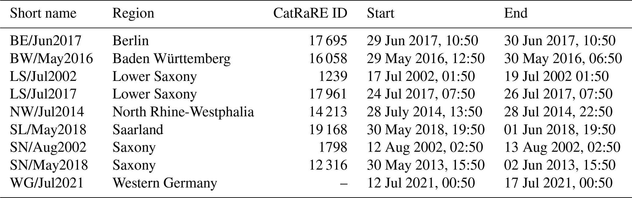
The DWD extracted more than 20 000 HPEs with durations between 1 h and 72 h from 20 years of radar data (RADKLIM) in Germany. Each HPE is listed with parameters such as date, time, duration, mean and maximum precipitation, severity indices, and geographical and demographical information. There are two versions of the catalog that use different thresholds (exceedance of warning level three for severe precipitation by the DWD and the exceedance of a return period of 5 years). The catalog is updated every year and is openly available (Lengfeld et al., 2021b). The WEI was used to determine the most extreme duration level of an event and is one of the attributes listed in CatRaRE. For this study, we used the CatRaRE version that is based on the exceedance of warning level three (25 mm in 1 h or 35 mm in 6 h; CatRaRE_2001_2020_W3_Eta_v2021_01) as an objective basis to select the 100 most extreme precipitation events in Germany between 2001 and 2020. Nine HPEs will be specifically discussed in this study and are hence detailed in Table 1.

Table 1 Events used for case studies. The short name was constructed from an acronym that specifies the region in which the event occurred (mostly the federal state), the month, and the year.

3 Methods

In this study we evaluate HPEs based on the WEI by Müller and Kaspar (2014) and extend this index to represent extremeness across spatiotemporal scales. We will refer to this as the cross-scale weather extremity index, xWEI. As both indices are based on the calculation of return periods and therefore rely on extreme value statistics, we will first describe the three different methods we used to derive the parameters for the GEV distribution and then outline the calculation of WEI and xWEI. The process is as follows.

1. Calculate the parameters of the GEV distribution for each pixel in the RADKLIM_RW_2017.002 dataset with different methods (cell-wise GEV, region of interest, duration-dependent GEV distribution).

2. Evaluate 101 selected HPEs using the WEI and xWEI based on each method of GEV parameter estimation.

3. Select events for case studies based on ranking results.

3.1 Calculation of return periods

WEI and xWEI require return periods for each pixel and each duration in the spatial domain. We estimated return periods for each pixel of the RADOLAN grid using the GEV distribution, which was found to be suitable for modeling precipitation extremes (Fowler and Kilsby, 2003) and which was used in previous studies that applied the WEI (Gvoždíková et al., 2019; Minářová et al., 2018; Müller and Kaspar, 2014). While Müller and Kaspar (2014) proposed an interpolation of return periods derived from station data to a grid, we instead use gridded precipitation data and perform cell-wise extreme value statistics to derive return periods. This way we avoid the uncertain interpolation, yet the time series used for estimating the GEV parameters are comparatively short (20 years). To address this issue, we compared different methods that help improve the robustness of the parameter estimation, all of which are based on the annual maximum values for each duration and each grid cell.

1. As a reference method, we fitted the GEV distribution to the series of annual maxima for each cell and each duration with the R package “extRemes” (Gilleland and Katz, 2016).

2. Region of interest (ROI): we included information from neighboring cells to make the GEV parameter estimation more robust towards small-scale variability in the RADKLIM_RW_2017.002 dataset. The series of annual maxima from the pixels in a 19 × 19 km box around the pixel of interest are weighted by distance to the center and are included in the estimation of the GEV parameters for this pixel. This method, described in detail in Burn (1990), was also used by Müller and Kaspar (2014).

3. Alternatively, we took advantage of the parameter dependence between different durations in order to make the parameter estimation more robust (Koutsoyiannis et al., 1998). While the reference approach fits the GEV parameters independently for each duration, this approach introduces a duration-dependent scale and location parameter in the GEV distribution, which is then estimated simultaneously for all durations. This approach is considered consistent because it prevents the crossing of quantiles (Fauer et al., 2021), but it is also computationally more efficient. To fit the parameters for this duration-dependent GEV (dGEV) distribution for each pixel we used the R package “IDF” by Ulrich et al. (2019).

3.2 Calculation of WEI

The WEI is based on the assumption that increased extremeness of an event is either due to an increase in intensity or an increase in spatial extent. Hence, the WEI is a measure of rarity and spatial extent (Müller and Kaspar, 2014). For a specific duration and a fixed spatial domain, we compute an event's return period for each pixel and sort the pixels in descending order based on their return period. The maximum considered return period was set to 1000 years following the example of Müller and Kaspar (2014). We will refer to the following exemplary event, shown in Fig. 1, which lasts 4 h and for which the E_tA is calculated for four durations $t_{\mathrm{1},\mathrm{\dots },\mathrm{4}}$. This means that the E_tA is calculated for every hour and every duration: starting with the pixel that has the highest return period, we then successively add one more pixel with the next lower return period. For each set of pixels that results from this incremental process, we compute a measure of extremeness (Fig. 1). This measure, E_tA, quantifies the intensity (the average of the return periods) at a specific spatial extent (the number and size of pixels). More specifically, the extremeness E_tA for a duration t of a set of n pixels is the product of the mean of the common logarithm of the return periods p_t,i and a weighted measure of the area (for which Müller and Kaspar suggested the radius R of a circle whose area A is equal to the pixel group area). The radius R therefore represents a weighting function of the area. We will discuss the choice of this weighting function further in Sect. 4.3.1. The highest E_tA value found in this procedure is chosen to define the extremeness of the event (WEI).

$$\begin{array}{}\text{(2)}& E_{\mathrm{tA}}={\displaystyle \frac{{\sum }_{i=\mathrm{1}}^n\ln \left(p_{t,i}\right)}{n}}\cdot {\displaystyle \frac{\sqrt{A}}{\sqrt{\mathit{\pi }}}}\left[\ln \right(\mathrm{year}\left)\mathrm{km}\right]\end{array}$$

As the pixels are sorted, the average of the return periods continuously decreases with each pixel that is added, while the area A continuously increases. Hence, the extremeness E_tA increases as long as cells with high return periods are accumulated. At some point, when more and more pixels with lower return periods are added, the expanding area does not compensate for the decrease in the mean return period, thus leading to a decrease in E_tA. E_tA curves are then calculated for each duration t of interest (Eq. 2) and for each hour (moving window for durations longer than 1 h) of the event. The WEI is the maximum E_tA value found during this procedure. This way the most extreme duration and the spatial extent of an event can be estimated (Fig. 1).

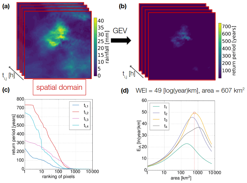
Figure 1 Explanation of the WEI. (a) Rasters with rainfall intensities at duration t_i for a spatial domain (red) that captures an HPE for each hour (t_i,1–t_i,4) of the event. (b) For each pixel and for each time step ($j=\mathrm{1},\mathrm{\dots },\mathrm{4}$), the return period is calculated. (c) The pixels are sorted by return period in descending order. (d) For each group of ranked pixels, E_tA is calculated. The steps in (b) to (d) are repeated for all durations t_i. In this exemplary case with four time steps and four durations ($i=\mathrm{1},\mathrm{\dots },\mathrm{4}$), this results in 16 E_tA curves. Panel (d) shows only the E_tA curve with the highest maxima for each duration $t_{\mathrm{1},\mathrm{\dots },\mathrm{4}}$. The maximum of all the resulting curves is the WEI (49 [ln(year)km], encircled in red). The maximum was achieved at t₃ at a spatial extent of 607 km².

3.3 The cross-scale weather extremity index

The calculation of the proposed cross-scale index, xWEI, directly builds on the procedure to compute the WEI (see Sect. 3.2). We just interpret the E_tA curves differently. Each E_tA curve displays how the extremeness of an event extends across spatial scales. Hence, such a curve contains more information than just the maximum value (Fig. 2a): the distribution of E_tA across scales. The curve informs us whether E_tA is high across a larger range of spatial scales (i.e., areas) or whether high values are rather limited to a specific spatial scale. Consequently, the extremeness of an event across spatial scales could be described by the integral of the E_tA curve (Fig. 2b). Analogously, we can also integrate E_tA across durations in order to measure by how much the extremeness extends across temporal scales. If the E_tA curves are represented by a two-dimensional grid along the dimensions area [km²] and duration [h], the E_tA curves define a surface that illustrates the extremeness of an event across spatial and temporal scales (Fig. 2c). Even though it is computationally more demanding, we chose to interpolate a surface instead of just summing up the integrals of the individual curves (Fig. 1) to ensure that we seamlessly represent all possible durations and to avoid overemphasizing the arbitrary choice of specific duration levels. Furthermore, we consider the volume under the surface to be a more intuitive representation of the index. To ensure that we do not overemphasize long durations in the integral, we used the natural logarithm of the duration. We propose that the volume underneath this surface represents the cross-scale extremeness of an HPE and can be used as a corresponding index, which we refer to as xWEI. Formally, xWEI corresponds to the double integral of E_tA over ln (t) and A.

$$\begin{array}{}\text{(3)}& \mathrm{xWEI}=\underset{\ln \left(t\right)}{\int }\underset{A}{\int }{E}_{\mathrm{tA}}\mathrm{d}A\mathrm{d}\left(\ln \right(t\left)\right)\end{array}$$

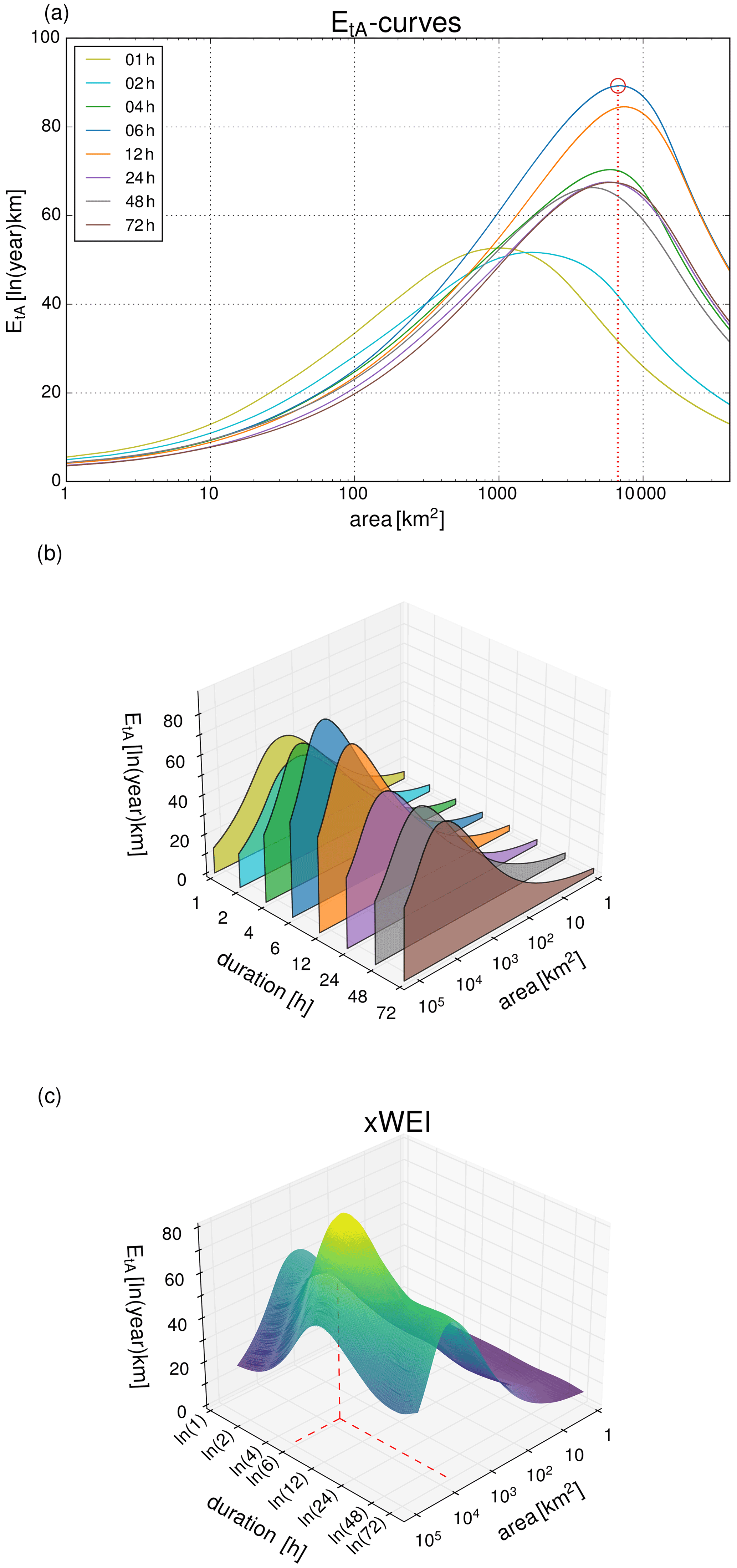
Figure 2 (a) E_tA curves for different durations plotted along the spatial dimension (area), with the WEI marked by a red circle. (b) The same E_tA curves as in (a), but aligned along the temporal dimension (duration). (c) E_tA values from (b) interpolated on a regular grid of logarithmic values of durations and area. All plots display the same extreme precipitation event (NW/Jul2014).

3.4 Choosing the size of the spatial domain

WEI and xWEI can be computed for arbitrarily defined spatial domains. The selection of the domain is a subjective decision to be made by the user and could have an essential impact on the resulting values of WEI and xWEI. Müller and Kaspar (2014) selected the whole country of the Czech Republic as a spatial domain. Lengfeld et al. (2021a) computed the WEI for groups of contiguous grid cells for which a specific precipitation threshold was exceeded.

In general, WEI and xWEI of different events are comparable only if the size and shape of the spatial domain are the same across events. The location of the spatial domain can be fixed (e.g., in the case of a country or a river basin), but it could also vary in space in the case that we want to compare events that took place in different parts of a larger region (e.g., a large country, continent, or model domain). The latter applies to our study in which we compare events that occurred in different parts of Germany. As we are most interested in the cross-scale extremeness of precipitation events in relation to compound inland flooding and disaster response, we did not compute WEI and xWEI for the entire spatial RADKLIM domain of 1100 × 900 km. Instead, we used the centroid of each event selected from the CatRaRE (see Sect. 2.2) and then chose a 200 × 200 km window around that centroid as the spatial domain to compute WEI and xWEI. While this is an arbitrary choice, we considered this size to be an adequate compromise: it is large enough to capture properties that are relevant for the generation of large river floods but small enough so that small-scale intense precipitation features (relevant for pluvial and flash floods) are not outweighed by large-scale features. It is possible that events are not fully captured by this window shape and size, but to keep events comparable we decided to stick to a uniform window for all events. Events which are located close to the national border of Germany contain more missing rainfall values, which adds uncertainty to the evaluation of these events. In some cases the centroid of the event was outside the national border of Germany. In this case we moved the centroid to the closest pixel with higher rainfall and thereby shifted the spatial domain of the event slightly inside the borders of Germany. Potential implications of such choices are discussed in Sect. 4.3.2.

3.5 Ranking of extreme events

In order to demonstrate the informational value and the behavior of the cross-scale index, xWEI, in comparison to the established WEI, we analyzed the 100 HPEs with the highest WEI in the CatRaRE. The event WG/Jul2021, which caused the floods in western Germany in July 2021, was added to this list although it was not yet included in the catalog, leading to a total of 101 analyzed events. We only used the CatRaRE to select events, but we computed both WEI and xWEI uniformly based on our above definition of the spatial domain of analysis. Both WEI and xWEI were then used to rank the events and to compare both rankings. Furthermore, we investigated how the choice of the GEV parameter estimation method (Sect. 3.1) affected the computation of WEI and xWEI and hence the ranking results.

4 Results and discussion

4.1 Effects of GEV parameter estimation method, ranking of events

We calculated the WEI and xWEI for 101 HPEs. Figure 3 shows the corresponding rankings with regard to both indices. Before we discuss whether and how these rankings depend on the choice of one of the two indices, we would like to briefly evaluate the sensitivity of the indices to the method to estimate the GEV parameters. The calculation of WEI and xWEI is based on calculating the return periods for each duration and each grid cell which is affected by the event. We used three different methods to derive the return periods (cell-wise fitting of GEV distribution, region of interest, and duration-dependent GEV distribution). Figure 3 shows the xWEI results for each estimation method and each of the 101 evaluated HPEs. Generally, all three methods lead to very similar results for WEI and xWEI. The xWEI and WEI values achieved with the cell-wise GEV method deviate most from the results of the other two methods, while the results of the ROI method and the dGEV are more similar. This is presumably caused by the fact that the GEV method is less robust, as parameters are estimated separately for each grid cell and duration. This could affect the ranking, especially for the lower ranks, which is why we discarded this method. The differences between ROI and dGEV are less pronounced. However, we chose the results obtained from the dGEV method for all of the following analysis. This way, we avoid inconsistencies across durations (such as quantile crossing, see Koutsoyiannis et al., 1998), which is an important feature for the computation of WEI and xWEI (both indices put return periods from different durations into one context).

Figure 3 (a) Ranking the 101 most extreme precipitation events according to CatRaRE based on the novel xWEI. The xWEI was calculated with three different methods: cell-wise GEV (blue), region of interest (ROI, red), and duration-dependent GEV (dGEV, black). The ranking was carried out based on the values obtained from the dGEV method. (b) Comparison of dGEV and ROI methods for the calculation of xWEI. (c) Comparison of dGEV and cell-wise GEV. (d) Ranking the 101 most extreme precipitation events according to CatRaRE based on the WEI. (e) Comparison of dGEV and ROI methods for the calculation of WEI. (f) Comparison of dGEV and cell-wise GEV methods for the calculation of WEI.

With regard to the ranking of events, the WG/Jul2021 event stands out as the most extreme event for both WEI and xWEI. Uncertainty regarding this result arises from the fact that the year 2021 was not included in the calculation of the GEV parameters because the reprocessed RADOLAN data were not yet available (see Sect. 2.1). For this reason, it is possible that the extremeness of the event was overestimated. Furthermore, the events SN/Aug2002, BE/Jun2017, LS/Jul2017, and LS/Jul2002 are ranked among the six most extreme events for both the WEI and xWEI. Interestingly, the LS/Jul2017 (WEI rank: 2, xWEI rank: 6) event outranks the famous SN/Aug2002 event that flooded the city of Dresden (WEI rank: 3, xWEI rank: 2) when ranked by the WEI. However, we need to be aware that the SN/Aug2002 event might not have been captured in its full extent by the RADKLIM data as it also affected significant parts of the Czech Republic (Müller et al., 2015). Figure 4 shows four of the highest-ranking events with regard to xWEI. The surfaces illustrate the cross-scale extremeness of these events, but they also illustrate, in comparison, the unique level of extremeness of the WG/Jul2021 event.

Figure 4 Comparison of xWEI for four high-ranking HPEs. WG/Jul2021 (a), SN/Aug2002 (b), BE/Jun2017 (c), BW/May2016 (d). The red lines indicate the spatial and temporal scale at which the event reached its maximum extremeness.

In this study, however, we are specifically interested in events for which the rank substantially differs between WEI and xWEI. The BW/May2016 event, for instance, caused a series of devastating flash floods in southwestern Germany, including the notorious flash flood in the village of Braunsbach (Bronstert et al., 2018): this event is ranked at position 19 using the WEI but among the top five events based on the xWEI. Figure 5a provides a more systematic representation of how the ranks change subject to the chosen index. The mean absolute deviation between the two rankings is 18 ranks. For 60 events, the ranks based on WEI and xWEI deviate by 10 ranks or more, for 39 events by 20 ranks or more, and for 10 events by 40 ranks or more; the maximum difference is 65 ranks (SN/May2013). To better understand these differences, we selected two case studies: for case study 1, the rank based on xWEI is lower than the respective WEI rank by 47 points (event SL/May2018, see Sect. 4.2.1); for case study 2, it is higher by 65 points (event SN/May2013, see Sect. 4.2.2).

Figure 5 (a) The xWEI ranks plotted over WEI ranks. Please note that the values on both axes are decreasing in order to enhance the comparability to panel (b), which shows xWEI values plotted over WEI values.

Surely, we need to be aware that a small change in the index value could cause a notable change in rank, specifically beyond the “top 10” ranks with the curves in Fig. 3 being less steep. Hence, the rankings and their comparison, are, to some extent, sensitive to random effects. Still, Fig. 5b confirms that the scatter which we observe in Fig. 5a is not just caused by small differences in the index values, but also that plotting xWEI over WEI exhibits considerable scatter.

4.2 Case studies

4.2.1 Case study 1: SL/May2018

In the night from 30 May to 1 June 2018, the small towns of Kleinblittersdorf, Bliesransbach, and St. Ingbert in the federal state of Saarland were hit by a flash flood that also carried a lot of sediment and debris, hence causing essential damage. The event's rank based on WEI is 65; based on xWEI, it is 18 – the difference in ranks is hence 47. How can we explain such a difference? The plot of the E_tA surface (Fig. 6) reveals that this HPE was extreme across temporal scales. For all durations, the maximum E_tA values were high (Table 2) and even exhibited two local maxima, one around 4–6 h and one around 48 h duration with the maximum E_tA at a spatial extent of 5377 km². In total, that leads to a large volume under the surface spanned by the E_tA curves (Fig. 6). The resulting xWEI is 1745 [–]. The fact that this event was obviously not only extreme at a duration of around 4 h is not captured by the WEI. Lengfeld et al. (2021a) mention another event in a case study that caused considerable damage in the city of Münster (NW/Jul2014, Fig. 1), which was evaluated with a surprisingly low WEI in CatRaRE. Although this event is not included in the original top 101 HPEs in CatRaRE, we re-evaluated this event with WEI and xWEI. Due to the extremeness on various scales, the xWEI would have ranked this event in the top 100 HPEs of CatRaRE (rank 76) and evaluated this event as more extreme than the WEI (xWEI: 1017, WEI: 68 [ln(year)km]). Because our WEI value for this event would have also ranked it in the top 100 of CatRaRE (rank 96), we have to consider that our approach regarding the selection of the spatial domain of an event differs from the method chosen in CatRaRE (connected cells), which also affects the evaluation of the extremeness of events.

Table 2 Maximum E_tA values for all considered durations. The WEI of this event (the maximum E_tA value regarding all durations) is in bold.

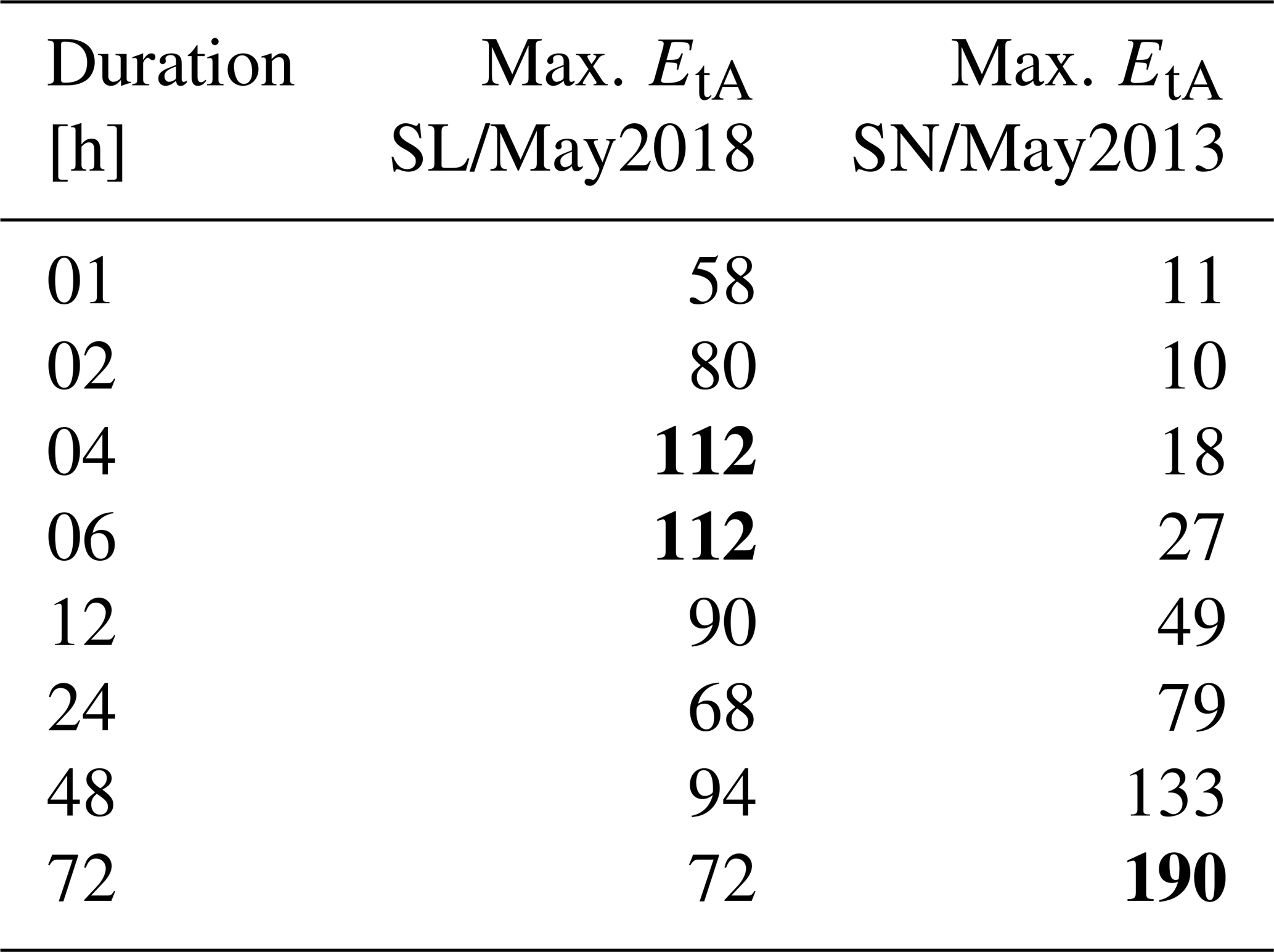
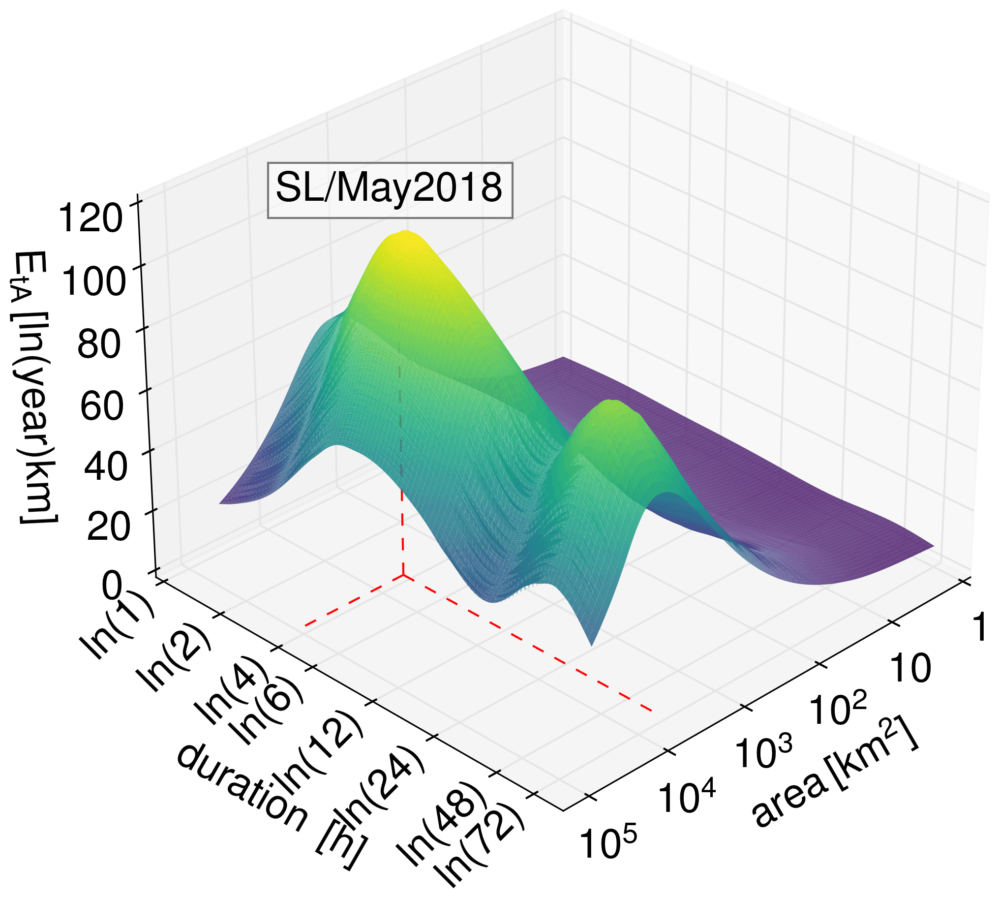
Figure 6 Kleinblittersdorf, Saarland, May 2018 (SL/May2018). Surface defined by E_tA curves. The red lines indicate the spatial and temporal scale at which the event reached its maximum extremeness.

4.2.2 Case study 2: SN/May2013

The second case study shows different cross-scale characteristics compared to the first. This event lasted from the 30 May to 2 June 2013, with its center in Steinberg/Saxony, and shows extreme precipitation at rather longer durations, with the maximum E_tA value observed at the longest analyzed duration of 72 h (Table 2 and Fig. 7) and an area of 18 211 km². The WEI rank for this event is 14, while the xWEI rank is 79. During this event, extreme precipitation on sub-daily timescales is less pronounced. Compared to the SL/May2018 event (case study 1), the maximum E_tA values for the durations 1–6 h are relatively low; the xWEI for this event is 993 [–]. The maximum E_tA at 72 h is represented by WEI (190 [ln(year)km]). Based on WEI, this event ranks higher than the BW/May2016 event (WEI: 176 [ln(year)km]) and the SL/May2018 event (case study 1, WEI: 112 [ln(year)km]). But the xWEI for these events tells a different story: the xWEI for the BW/May2016 event (2326 [–]) is 2.3 times higher and the WEI for the SL/May2018 event (WEI: 1745 [–]) is 1.7 times higher than the WEI for the SN/May2013 event (WEI: 993 [–]). While the SN/May2013 event (case study 2) did not show extremeness across temporal scales, the BW/May2016 event was extreme on all temporal scales with E_tA maxima ranging from 60 (1 h duration) to 176 (12 h). Similarly, but less pronounced, this can be observed for the SL/May2018 event.

Figure 7 Steinberg, Saxony, May 2013 (SN/May2013). Surface defined by E_tA curves. The red lines indicate the spatial and temporal scale at which the event reached its maximum extremeness.

4.3 Required parameter choices for the computation of E_tA, WEI, and xWEI

In this section, we will discuss three parameters that affect the computation of E_tA, WEI, and xWEI and which need to be set by users interested in quantifying the cross-scale extremity of precipitation events. These parameters are the weight of the area in the computation of E_tA, the choice of the spatial domain of analysis, and the choice of duration levels.

4.3.1 Weighting the spatial extent of an event

According to Müller and Kaspar (2014), the WEI is the product of a measure of rarity (mean return periods) and a measure of the spatial extent (or area). To avoid the E_tA curves continuously growing with increasing area A, the authors suggested representing the spatial extent by the radius $\frac{\sqrt{A}}{\mathit{\pi }}$ of an imaginary circle with area A (see Eq. 2). While this is an intuitive and illustrative way to reduce the weight of the area, we need to be aware that the decision to weight the area based on $\frac{\sqrt{A}}{\mathit{\pi }}$ is arbitrary. Weighting the spatial extent differently will change the resulting values of WEI and xWEI and hence the corresponding rankings. This arbitrariness should, however, be seen as an opportunity to express preferences with regard to the spatial scale of interest: if we are more interested in local impacts such as flash floods, it might be informative to put less weight on the size of the affected area and thus more weight on cells with high-intensity rainfall. This could, for example, be achieved by replacing A with ln (A) when calculating E_tA instead of the radius R.

Figure 8 demonstrates how such a choice affects the resulting ranks. While the results are quite similar for the top 10 ranks, we can observe deviations of 26 ranks for the xWEI and up to 59 ranks for the WEI (not shown).

Figure 8 The xWEIs compared with each other for two different methods of weighting the area for the calculation of E_tA. The xWEI rank describes the weighting proposed by Müller and Kaspar (2014). xWEI_mod was calculated by using the natural logarithm of the area when calculating E_tA.

4.3.2 Setting the spatial domain of analysis

In our analysis, we used a square of 200 × 200 km around the event centroid in order to define the spatial domain for which the E_tA curves as well as WEI and xWEI were computed for each event. Generally, we observed that most high-ranking HPEs affected a large spatial domain and that, for many events, E_tA does converge towards zero for very large spatial extents (see, e.g., Fig. 4 for the most extreme events). In Sect. 4.3.1, we already discussed the role of weighting the spatial extent of an event when computing E_tA. Decreasing the weight of the spatial extent, e.g., by using ln (A) instead of A, will probably make the falling limbs of the E_tA curves steeper and enhance the convergence of E_tA to values of zero with increasing spatial extent. For many events, though, the value of xWEI will grow further if we increase the spatial domain of analysis. Furthermore, the square shape of the spatial domain might not be an optimal choice to appreciate the extremity of elongated precipitation structures as they, e.g., occur along frontal lines. The seemingly arbitrary choice of the spatial domain of analysis could once more be considered an opportunity to consider user preferences: while in the present study we followed the aim of detecting and ranking events across the entire RADKLIM domain, the definition of the spatial domain might be more evident in other contexts. For example, the choice might be a river basin (see, e.g., Gvoždíková et al., 2019) or an administrative unit within which resources for disaster response are managed. Once fixed, the spatial domain provides a valid frame to compare the cross-scale extremeness of different events up to a maximum spatial scale of interest. In the context of the spatial domain, we also need to be aware that the resulting indices might not represent the full level of extremeness in the case that the spatial domain of analysis is partly outside the spatial domain for which observations are available. For example, the WG/Jul2021 event extended considerably towards Belgium so that parts of the event were not captured by the radar composite (RADKLIM) of the DWD. The same applies to the SN/Aug2002 event, which extended far into the Czech Republic. In fact, we need to acknowledge that the extremeness of events close to the edges of the dataset will, on average, be systematically underestimated. We still decided for this study not to discard events that occurred close to the German borders – otherwise, some of the most important events would be entirely missing. Future research, however, could attempt to quantify the systematic errors that are introduced by edge effects.

4.3.3 Selection and weighting of duration levels

Similar to the above issues of weighting the spatial extent and setting the spatial domain of analysis, the choice of the maximum duration as well as the choice and weighting of duration levels up to this maximum are subject to arbitrariness, or, in other words, to user preferences. This issue is more delicate for the computation of xWEI than for the computation of WEI: E_tA is a function of spatial extent and duration, and as long as the maximum analyzed duration is large enough to detect a local maximum of E_tA, the computation of WEI is not a problem. The value of xWEI, however, will not converge but grow further with increasing duration levels for as long as E_tA does not converge to zero. And even if we chose the maximum duration level large enough for E_tA to converge, we need to decide how to integrate E_tA over different duration levels in order to compute xWEI. Imagine we analyzed all duration levels from 1 to 72 h with an increment of 1 h: in that case, we would have 72 nodes along the duration dimension, only 24 of which would represent extremeness at sub-daily timescales. This imbalance would overemphasize E_tA values at long durations in the resulting estimate of xWEI. In the present study, we decided to use 72 h as the maximum duration and to integrate E_tA along the natural logarithm of duration levels (see Sect. 3.3). That way, the E_tA curves for all durations are almost evenly spaced on the two-dimensional grid. Still, users might prefer a different maximum duration and also a different conversion of duration values for the step of integration (which effectively corresponds to putting different weights to different duration levels).

5 Conclusions and outlook

The WEI as suggested by Müller and Kaspar (2014) represents the extremeness of an event at the spatial and temporal scale at which the extremeness reaches its maximum. While such a maximum typically exists, the extremeness of an event can extend across multiple scales – an important property that is not represented by the original WEI. The proposed cross-scale index, xWEI, is able to capture cross-scale extremeness in space and time. Accordingly, HPEs might be ranked very differently depending on which index, WEI or xWEI, is used. While we do not recommend replacing the original WEI, we are confident that the novel xWEI can provide valuable complementary information with regard to potential impacts of HPEs. As the computational steps towards the establishment of the underlying E_tA curves are the same for the WEI and xWEI, the added cost of retrieving xWEI on top of WEI is negligible compared to the informational benefit.

In our study, we demonstrated the application and behavior of the xWEI in comparison to the WEI for a set of 101 extreme precipitation events from 2001 to 2021 based on hourly radar-based precipitation composite data from the DWD (RADKLIM, RADOLAN, Sect. 4.1). We found that, based on current data, the disastrous July 2021 precipitation event in western Germany stood out with regard to both WEI and xWEI. This similarly applies to other high-ranking events: in our analysis, the events BE/Jun2017, SN/Aug2002, and LS/Jul2002 ranked among the top five for both WEI and xWEI. Other events were rated as considerably more extreme based on the xWEI. Several among these events have become infamous for causing essential damage (e.g., BW/May2016, SL/May2018, and NW/Jul2014 events). As described by Thieken et al. (2022), such damage is often caused by compound inland floods. Once the reprocessed RADOLAN data for the year 2021 are available, the year 2021 should be included in the extreme value statistics to ensure a consistent calculation for all events and for better comparability regarding the WG/Jul2021 event. Generally, we could show that the xWEI contains important information about the cross-scale extremeness of HPEs and could thus be used as complementary to the WEI, which gives information only about the maximum extent and the most extreme duration. The xWEI could be a suitable instrument to describe the potential of an HPE to cause impacts, such as floods, and future studies should investigate this potential by systematically linking the WEI and xWEI to observed impacts and damage inventories. To extend the limited scope of this study, future applications should aim at a comprehensive detection and ranking of extreme events from the RADKLIM dataset or other similar datasets. That way, we might possibly find events with a very high xWEI which were not yet represented in the 100 events selected for the present study (based on the CatRaRE). The method as described in this study is applicable to any multi-annual gridded time series of precipitation with high resolution in space and time, including radar data and regional climate models. Apart from the need to explore the informational value of this novel index in more comprehensive application studies, prospective research should further scrutinize and develop the theoretical foundations of both WEI and xWEI, as well as explore the role of subjective choices in the computation of these indices. That particularly applies to the following.

• The definition of the spatial domain. In this study, the spatial domain was a window of 200×200 km, the center of which varied across the RADKLIM domain. Other window sizes could be used depending on user preferences (see Sects. 3.4 and 4.3.2). In general, the spatial domain should be adjusted to the underlying study objectives: e.g., users could choose the fixed area of a specific river catchment or an administrative unit that accounts for specific tasks of disaster response.

• The minimum and maximum duration. In the present study, the maximum duration was set to 72 h according to the standards for extreme value statistics established at the DWD. In analogy to the size of the spatial domain reflecting the maximum spatial scale of interest, the maximum duration level reflects the maximum temporal scale of interest and could be set accordingly based on user preferences. The minimum duration level was set to 1 h but could be reduced, at least with the RADKLIM data, to 5 min. Accounting for sub-hourly durations might shed new light on processes related to pluvial and flash floods, as well as to erosion and landslides.

• Representing the spatial extent for computing. E_tA represents the product of rarity and spatial extent. Müller and Kaspar (2014) represented the spatial extent by the radius of a circle with an equivalent area. While this is illustrative, other transformations of the area are conceivable. For example, the natural logarithm of the area would put more emphasis on smaller spatial extents and cause the E_tA curves to drop at a higher rate with increasing spatial extents (see Sect. 4.3.1).

• Weighting spatial extent and duration. This computational step is specific to xWEI; for the computation of WEI, we only need to retrieve the maximum value of E_tA across duration and spatial extent. For xWEI, however, we need to compute the integral of E_tA along two dimensions. We noticed that high values of E_tA often come along with long durations and large extents. Using different transformations along these two dimensions could put more emphasis on smaller scales (see Sect. 4.3.3 and 4.3.1). Furthermore, it would be more consistent and hence preferable to use the same representation of spatial extent (e.g., the natural logarithm) for the computation of E_tA and for the integration of E_tA.

Combining a more comprehensive retrieval and comparison of WEI and xWEI (from RADKLIM or other data) with an improvement of the theoretical and computational foundations of these indices might open the way to better understand how the scaling properties of extreme precipitation affect the interaction of processes in compound events and how they might affect the processes of disaster risk management across scales.