Estimating return intervals for extreme climate conditions related to winter disasters and livestock mortality in Mongolia

Mass livestock mortality events during severe winters, a phenomenon that Mongolians call dzud, cause the country significant socioeconomic problems. Dzud is an example of a compound event, meaning that multiple climatic and social drivers contribute to the risk of occurrence. Existing studies argue that the frequency and intensity of dzud events are rising due to the combined effects of climate change and variability, most notably summer drought and severe winter conditions, on top of socioeconomic dynamics such as overgrazing. Summer droughts are a precondition for dzud because scarce grasses cause malnutrition, making livestock more vulnerable to harsh winter conditions. However, studies investigating the association between climate and dzud typically look at a short time frame (i.e., after 1940), and few have investigated the risk or the recurrence of dzud over a century-scale climate record. This study aims to fill the gaps in technical knowledge about the recurrence probability of dzud by estimating the return periods of relevant climatic variables: summer drought conditions and winter minimum temperature. We divide the country into three regions (northwest, southwest, and east Mongolia) based on the mortality index at the soum (county) level. For droughts, our study uses as a proxy the tree-ring-reconstructed Palmer drought severity index (PDSI) for three regions between 1700–2013. For winter severity, our study uses observational data of winter minimum temperature after 1901 while inferring winter minimum temperature in Mongolia from instrumental data in Siberia that extend to the early 19th century. Using a generalized extreme value distribution with time-varying parameters, we find that the return periods of drought conditions vary over time, with variability increasing for all the regions. Winter temperature severity, however, does not change with time. The median temperature of the 100-year return period for winter minimum temperature in Mongolia over the past 300 years is estimated as −26.08 ^∘C for the southwest, −27.99 ^∘C for the northwest, and −25.31 ^∘C for the east. The co-occurrence of summer drought and winter severity increases in all the regions in the early 21st century. The analysis suggests that a continued trend in summer drought would lead to increased vulnerability and malnutrition. Prospects for climate index insurance for livestock are also discussed.

1 Introduction

1.1 Background

Mass livestock mortality induced by dry summers followed by unusually cold and/or snowy winters, known as dzud, causes problems for pastoral herding and the economy in Mongolia.¹ A total of 20 million livestock died of climate extremes from 2000–2002 and 2009–2010 (Rao et al., 2015). During the 2009–2010 dzud alone, approximately 20 % of the country's livestock population died, affecting 769 000 people, 28 % of the population in Mongolia (Middleton et al., 2015).

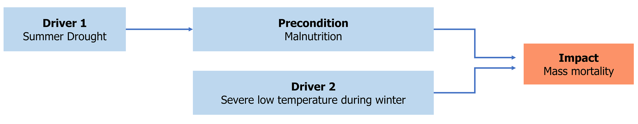
Dzud is a compound hazard, encompassing drought, heavy snowfall, extreme cold, and windstorms (Field, 2012). Dzud can cause mass livestock mortality, which leads to severe socioeconomic consequences such as unemployment, poverty, and mass migration from rural to urban areas (Dagvadorj et al., 2009; Kakinuma et al., 2019). The causes of dzud are complex. Increased livestock population and other land-use changes, such as urbanization and mining, are viewed as a major cause of the decline in pasture quality in the region (Bat-Oyun et al., 2016; Berger et al., 2013; Hilker et al., 2014). Among other socioeconomic factors, such as overgrazing, livestock mortality is caused and exacerbated by the following climate factors: summer drought, heavy snow, and high winds in concurrence with extreme cold winter temperature (Morinaga et al., 2003). Livestock mortality is strongly associated with winter (November–February) temperatures and prior summer (July–September) droughts (Rao et al., 2015) and precipitation (Tachiiri et al., 2008; Rao et al., 2015). For example, Rao et al. (2015) showed that a model based on winter temperature, summer drought, summer precipitation, and summer potential evapotranspiration explains 48.4 % of the entire variability in mortality. Extreme cold temperature, as well as exposure to storms or high winds, causes livestock to freeze to death, while heavy snow, ice, or drought prevents livestock from grazing and accessing fodder, which results in weakening immune system responses and starvation (Begzsuren et al., 2004; Fernandez-Gimenez et al., 2012; Morinaga et al., 2003; Rao et al., 2015). In addition to extreme winter temperature and snowfall, summer drought is an important driver because droughts deteriorate grazing and prevent livestock from surviving during severe winters (Begzsuren et al., 2004; Rao et al., 2015; Tachiiri et al., 2008). For example, the climate factors that contributed to the dzud in 1999–2002 and 2009–2010 were summer drought followed by extreme cold and snowfall in winter (Field, 2012). In this case, summer drought is regarded as a preconditioning factor for the dzud as a compound event (Zscheischler et al., 2020) (Fig. 1).

Figure 1 Diagram showing dzud is a preconditioned compound event.

Understanding mechanisms and impacts of dzud and climate extremes has wider implications for sustainability in rangelands, which account for 50 % of Earth's land surface, where 40% of the world's populations reside (Fernandez-Gimenez et al., 2012; Reynolds et al., 2007). A better understanding of the climate drivers of dzud and extreme events is also critical for preventive and responsive measures, such as weather index insurance. Weather index insurance recently became widely available, and its indemnities are paid based on realizations of a weather index such as rainfall and temperature that are expected to be highly correlated with actual losses, rather than on actual losses experienced by the policyholder (Barnett and Mahul, 2007; Haraguchi and Lall, 2019; Haraguchi et al., 2016). The advantage of index insurance is that the predetermined index cannot be manipulated by third parties. Payment is faster than loss-based insurance because payment will be made once the predetermined index exceeds the threshold. In contrast, for loss-based insurance, an insurance company must assess losses before making payment, which requires labor and time. The lower transaction costs of index insurance can also make it a more affordable product for the purchaser and thus a more viable offering for the insurance provider. The Index-Based Livestock Insurance Program (IBLIP) was institutionalized in 2014 to respond to the extreme climate disasters by the government of Mongolia with help from the World Bank (Skees and Enkh-Amgalan, 2002; Mahul et al., 2015; Mahul and Skees, 2007).

Studies analyzing long-term variabilities in extreme climate conditions in Mongolia are still limited because there are few long-term instrumental records of climate in the region. The records that do exist are often not continuous and contain missing data. Though historical documents record the occurrence of dzud from the 19th century, changes in climate in Mongolia have been observed in instrumental records only since 1940 (Batima et al., 2005). Some studies have reported that the frequency of dzud has increased, such as after 1950 (Fernandez-Gimenez et al., 2012; Middleton et al., 2015) or after 2000 (Munkhjargal et al., 2020). Furthermore, another study concluded that dzud frequency is expected to increase with future climatic changes, while using the Coupled Model Intercomparison Project's climate models (Bayasgalan et al., 2009). Natsagdorj (2001) shows that the trends of drought and the dzud index, estimated by normalized monthly temperature and precipitation, are increasing. However, these studies are based on observational data of dzud, which are available only from about 1940. It is critical to extend the time horizon in order to improve the reliability of the return period estimation of catastrophic dzud and of the assertions of secular changes in the causal climate variables. Long-term climate proxies, such as tree rings, have the potential to do so by deriving recurrence periods of dzud and climate extremes, especially to improve index insurance products (Bell et al., 2013). Yet, one of the challenges of improving the reliability of recurrence estimations is the lack of scientific understanding of the historical trends of past climate events due to the short meteorological record (Mahul and Stutley, 2010; McSharry, 2014; Rao et al., 2015).

To improve risk analysis of dzud, the investigation of extreme distributions of climate extremes is critical. Studies using millennial-length tree-ring data reveal that temperatures in Mongolia in the late 1990s and early 2000s were extraordinary (D'Arrigo et al., 2001; Jacoby et al., 1996). Based on well-calibrated and verified millennial-length tree-ring reconstruction of summer temperatures, Davi et al. (2015, 2021) show that the recent warming trend since the 1990s is anomalous in the long-term context in Mongolia. In addition, the tree-ring-based reconstructed Palmer drought severity index (PDSI) is used to assess drought variability in the past (Davi et al., 2010; Hessl et al., 2018). However, studies that estimate probability distributions of extreme climatic events to improve the reliability of the return period estimation of dzud for risk analysis are still lacking. Here, we use the term “risk analysis” to refer to the analysis of the probability of an extreme event whose consequences could be substantial (Rootzén and Katz, 2013) but not the analysis where risk refers to the combination of the probability of an event and its associated expected losses.

1.2 Objectives of the study

The objective of this study is to conduct risk analysis for the climatic variables that cause dzud, namely summer drought followed by extreme cold temperature and snowfall, in Mongolia while attempting to improve the reliability of the return period estimation of dzud utilizing tree-ring proxies and historical data on climatic variables. The study also explores the implications of the risk analysis and return period estimation for index insurance using tree-ring data. To address these objectives, we posed the following research question: how can the reliability of the return period estimation of climate extremes be improved?

There are two important climatic variables to predict dzud: summer drought conditions and winter temperatures (Lall et al., 2016; Rao et al., 2015). Notably, this study estimates return periods of extreme drought conditions by using a tree-ring-based reconstructed PDSI using an updated version of the Monsoon Asia Drought Atlas or MADA that spans 1300–2005 CE (Cook et al., 2010). We also estimate return periods of extreme cold temperatures in Mongolia. Since temperature data in Mongolia are only available from the early to middle 20th century, we simulate them from meteorological data in neighboring Siberia, which has records that extend back to the late 1800s, through a statistical model presented here. Tree-ring-based temperature reconstructions in the region are typically limited to the summer growing season and do not capture winter temperatures.

In Mongolia, the term “dzud” refers to high livestock mortality (Fernandez-Gimenez et al., 2012; Morinaga et al., 2003); however, we use climate variables to determine risk rather than mortality because the mortality rate assumes that the size of the population does not matter. In fact, changes in livestock populations do matter since they can also be related to changes in socioeconomic factors, such as shortage of food supply, which can be related to non-climate factors. Other socioeconomic factors impact livestock herding loss, including the total number of animals and the density per square kilometer. These numbers drastically increased after a transition to private ownership in the 1990s (Johnson et al., 2006; Rao et al., 2015; Reading et al., 2006). The increased livestock population resulted in overgrazing and degradation of the grassland, a decrease in the grassland carrying capacity, and a high mortality rate (Bat-Oyun et al., 2016; Berger et al., 2013; Hilker et al., 2014; Liu et al., 2013).

In order to estimate a return period of an extreme climate event, extreme value theory (EVT) is useful (Cheng et al., 2014; Katz et al., 2002). There are ongoing debates about which methods are most suitable for estimating extremes, such as the return period and expected number of exceedances (Read and Vogel, 2015; Rootzén and Katz, 2013; Salas and Obeysekera, 2014). EVT informs us how to extrapolate a rare event which has not been experienced for a long time from existing observational data with a short record. EVT is a widely used method for estimating the probability of extreme hydroclimatic events (Katz, 2010; Leonard et al., 2014; Slater et al., 2021), such as floods (Prosdocimi et al., 2015; Willner et al., 2018), precipitation (Gao et al., 2018; Minářová et al., 2017), and compound events (Leonard et al., 2014). EVT helps us to formulate a risk management strategy by deriving a distribution of extreme climate events and estimating a possible extreme value for the future's preparedness. There are two main approaches in EVT: the block maximum approach and the threshold approach, which will be described in “Data and methodology”. The objectives of this study were to

1. estimate return periods of extreme drought conditions by using a reconstructed PDSI,

2. estimate return periods of extreme cold temperatures in Mongolia by using long-term instrumental data from Siberia.

Conventionally, a stationarity process is assumed to estimate return periods. Here, we consider the extension of the record by explicit dependence on tree-ring climate proxies. We examine how the return periods may change over time due to slowly and systematically changing climate conditions, persistence in the PDSI, or other climate records. Exploring the nonstationary approach to return periods and risk opens “many opportunities” (Salas and Obeysekera, 2014). This has the advantage of reducing the bias in the near-term projection, assessment of the return period, and recurrence interval associated with the event.

We also explore the utility of using long-term climate proxies in the context of index insurance (Bell et al., 2013). In general, the index used for index insurance must be scientifically objective and easily measurable. The IBLIP in Mongolia uses the mortality rate as the index. Our study provides insights into the long-term variations in the mortality rate due to climate with the goal of reducing the bias and the variance of the estimates of the probability of the index used, by identifying the trend and using a longer record, respectively.

2 Data and methodology

2.1 Data and preliminary analysis

2.1.1 Tree-ring-reconstructed PDSI

Data

The PDSI is a standardized index that ranges from −10 (dry) to +10 (wet) based on a water balance model, accounting for precipitation, evaporation, and soil moisture storage (Cook et al., 2010; Dai et al., 2004; Palmer, 1965).² In this study, tree-ring-reconstructed PDSI values from 1700 to 2013 are taken from an updated version of the Monsoon Asia Drought Atlas (MADA) (Cook et al., 2010). MADA is a seasonally resolved gridded spatial reconstruction of drought and pluvials in monsoon Asia over the last 700 years, derived from a network of tree-ring chronologies (Cook et al., 2010). MADA can also reveal the occurrence and severity of previously unknown monsoon droughts (Cook et al., 2010). We consider three regions (northwest, southwest, and east Mongolia) in Mongolia, as shown in Fig. 2, based on clusters proposed by previous studies (Lall et al., 2016). These spatial clusters are based on the mortality data at the soum (county) level from 1972 to 2010, using hierarchical clustering (Johnson, 1967), which were adjusted with the spatial patterns of the Mongolian topography, climate zones, and mean precipitation in growing seasons. It is reasonable to use these clusters because the objective of the study is to improve risk analysis of dzud and mortality of livestock in Mongolia.

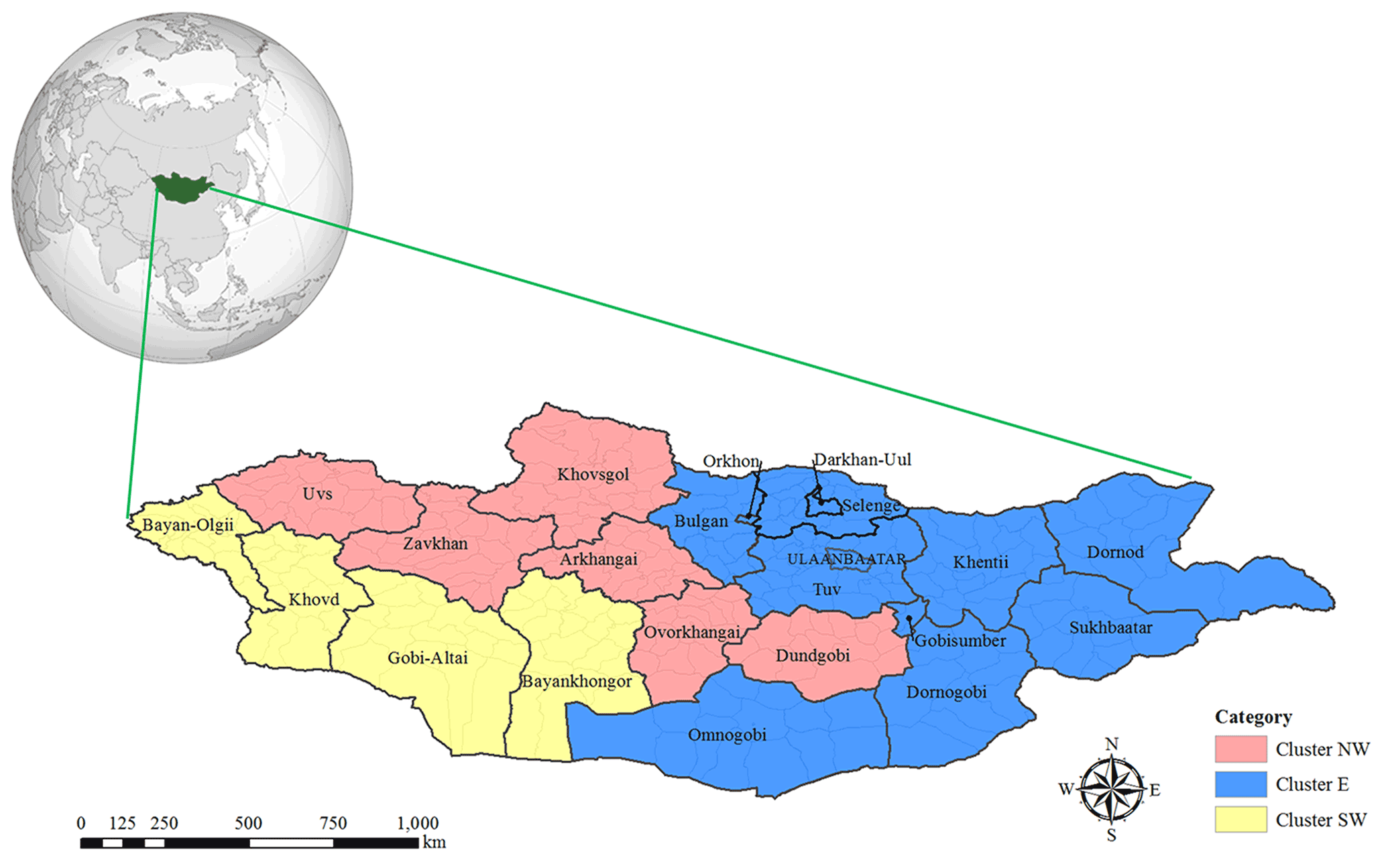
Figure 2 Spatial clusters of the mortality index based on 1972–2010 soum level mortality indices. Source: Lall et al (2016); https://en.wikipedia.org/wiki/File:Mongolia_(orthographic_projection).svg (last access: 19 June 2022).

Preliminary analysis

The correlation in PDSI values from 1700 to 2013 between three clusters is shown in Table 1. The Mann–Kendall trend test is used to examine the trends of the PDSI data (Kendall, 1948; Mann, 1945). The Mann–Kendall test shows that there are no monotonic trends in the PDSI data for all clusters (Table 1). Yet, time series of the tree-ring-reconstructed PDSI by clusters show that there is significant centennial-scale variability, which is important to consider since the time series suggest that there are persistent regimes that can last over decadal to centennial timescales (Fig. 3a–c). Though these may occur randomly or reflect systematic cyclical behavior, their consideration in a risk management strategy is critical.

Table 1 Mann–Kendall trend test and correlation coefficients of PDSI values from 1700 to 2013 between the three clusters.

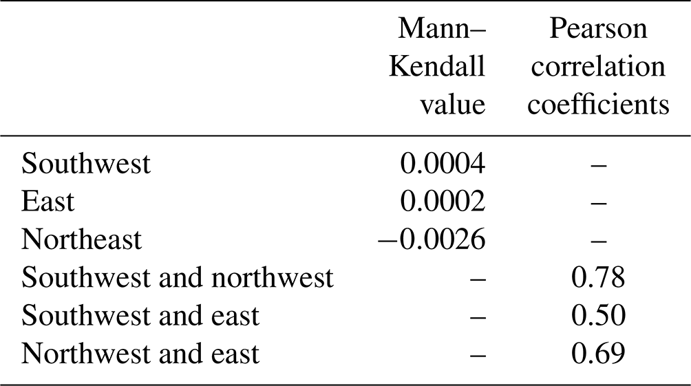
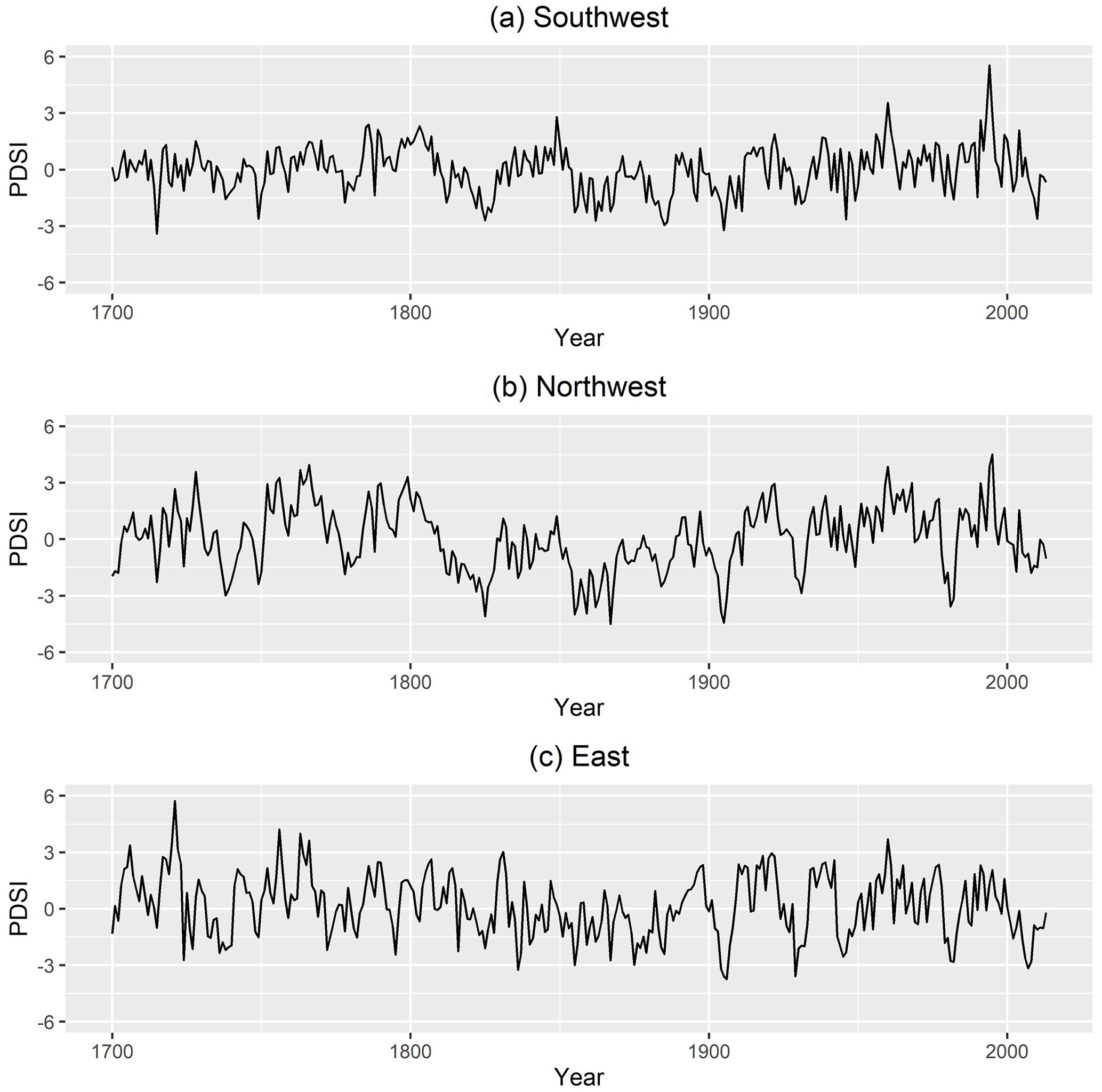
Figure 3 Time series of the tree-ring-reconstructed PDSI in (a) the southwest, (b) the northwest, and (c) the east clusters.

The autocorrelation function (ACF) and partial ACF of all the regions show that there are significant autocorrelations in the PDSI data in all clusters (in Figs. S1 and S2 in the Supplement). The development of a time series simulation model that uses these long lead correlations would help inform the risk analysis associated with the persistent regimes identified earlier. Autoregressive integrated moving average (ARIMA) models with different orders were evaluated based on the Bayesian information criterion (BIC), which can account for fitting errors for the Bayesian conditional mechanism of models. Please note that the BIC is a standard information-theoretic criterion whose relative magnitudes allow one to choose one model over another (Akaike, 1979; Burnham and Anderson, 2004). The order of the best ARIMA models in each cluster is (3, 0, 0) for the southwest, (1, 0, 2) for the northwest, and (1, 0, 0) for the east. These ARIMA models will be used later to forecast the effective return periods of droughts.

2.1.2 Climate variables

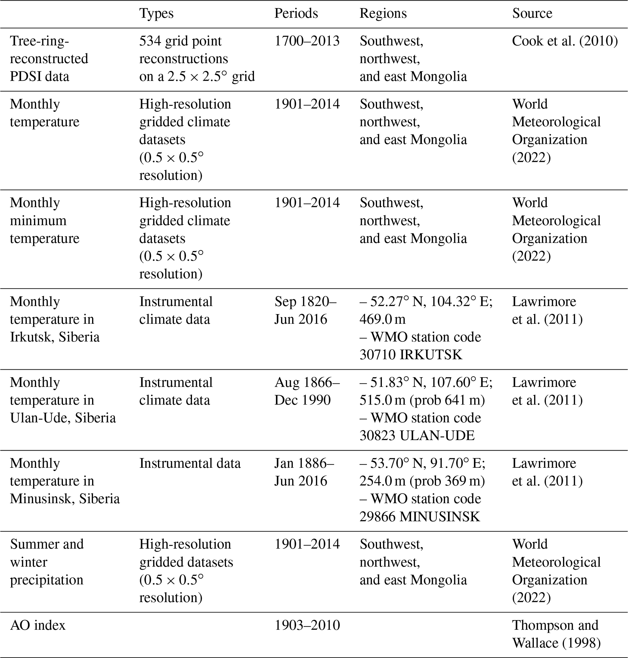
Models that use climate variables as covariates are explored for developing a nonstationary risk model. These data are summarized in Table 2. We use high-resolution gridded datasets of the Climate Research Unit (CRU) at the University of East Anglia for monthly temperature and summer (May–August) and winter (November–February) precipitation for the three clusters (Harris et al., 2014). All the gridded points within each cluster are averaged. We also used average monthly temperature data from instrumental records in Siberia, including Irkutsk (1882–2011), Minusinsk (1886–2011), and Ulan-Ude (1895–1989). We also use the Arctic Oscillation (AO) index (1903–2010), which comes from two sources: the Joint Institute for the Study of the Atmosphere and Ocean (JISAO) and the National Oceanic and Atmospheric Administration (NOAA) (Thompson and Wallace, 1998). The two records were merged into one record (e.g., Lall et al., 2016). The AO index is closely associated with summer and winter climates in East Asia (He et al., 2017). In particular, the negative phase of the AO is associated with more frequent cold-air outbreaks in East Asia, including Mongolia (Cohen et al., 2010; He et al., 2017; Yu et al., 2015). Finally, please note that although dry conditions of the PDSI are negative, all the analyzed PDSI values below are presented as reversed values (i.e., positive for dry conditions) because the R package, extRemes (Gilleland and Katz, 2016), will capture the maximum values.

Table 2 Data analyzed in this study. WMO denotes World Meteorological Organization.

2.2 Methodology

Extreme value analysis (EVA) is utilized in this study. In EVA, the distribution of many variables can be stabilized so that their extreme values asymptotically follow specific distribution functions (Coles et al., 2001). There are two primary ways to analyze extreme data. The first approach, the so-called block maxima approach, reduces the data by taking maxima of long-term block data, such as annual maxima (Coles et al., 2001). The generalized extreme value (GEV) distribution function is fitted to maxima of block data, as given by

$$\begin{array}{}\text{(1)}& G\left(z\right)=\exp \left[-{\left\{\mathrm{1}+\mathit{\epsilon }\left({\displaystyle \frac{z-\mathit{\mu }}{\mathit{\sigma }}}\right)\right\}}_{+}^{-\mathrm{1}/\mathit{\epsilon }}\right],\end{array}$$

where $y_{+}=\max \mathit{\{}y,\mathrm{0}\mathit{\}}$, σ>0, and $-\mathrm{\infty }<\mathit{\mu }$, ε<∞.

Equation (1)³ covers three types of distribution function depending on the sign of the shape parameter ε. The Fréchet distribution function is for ε>0, while the upper-bounded Weibull distribution function is for ε<0 (Gilleland and Katz, 2016). The Gumbel type is obtained in the limit as ε→0, which results in

$$\begin{array}{}\text{(2)}& G\left(z\right)=\exp \left[-\exp \left[-\left\{{\displaystyle \frac{z-\mathit{\mu }}{\mathit{\sigma }}}\right\}\right]\right],-\mathrm{\infty }<z<\mathrm{\infty }.\end{array}$$

The second approach, the so-called threshold excess approach, is to analyze excesses over a high threshold (Coles et al., 2001). The generalized Pareto distribution (GPD) has a theoretical justification for fitting to the threshold excess approach (Gilleland and Katz, 2016), as given by

$$\begin{array}{}\text{(3)}& H\left(x\right)=\mathrm{1}-{\left[\mathrm{1}+\mathit{\epsilon }\left({\displaystyle \frac{x-\mathit{\mu }}{{\mathit{\sigma }}_{\mathit{\mu }}}}\right)\right]}_{+}^{-\mathrm{1}/\mathit{\epsilon }},\end{array}$$

where μ is a high threshold, x>μ, scale parameter σ_μ>0, and shape parameter $-\mathrm{\infty }<\mathit{\epsilon }<\mathrm{\infty }$. The shape parameter ε determines three types of distribution function: heavy-tailed Pareto when ε>0, upper-bounded beta when ε<0; and the exponential obtained by taking the limit as ε→0, which gives

$$\begin{array}{}\text{(4)}& H\left(x\right)=\mathrm{1}-e^{-(x-\mathit{\mu })/\mathit{\sigma }}.\end{array}$$

The extreme value models can be applied in the presence of temporal dependence (Coles et al., 2001), as given below:

$$\begin{array}{}\text{(5)}& Zt\sim \mathrm{GEV}\left(\mathit{\mu }\right(t),\mathit{\sigma }(t),\mathit{\epsilon }(t\left)\right),\end{array}$$

where

$$\begin{array}{ll}{\displaystyle }& {\displaystyle }\mathit{\mu }\left(t\right)={\mathit{\alpha }}_{\mathrm{0}}+{\mathit{\alpha }}_{\mathrm{1}}t+{\mathit{\alpha }}_{\mathrm{2}}{t}^{\mathrm{2}}+\mathrm{\dots }+{\mathit{\alpha }}_n{t}^n,\\ {\displaystyle }& {\displaystyle }\mathit{\sigma }\left(t\right)=\exp \left({\mathit{\beta }}_{\mathrm{0}}+{\mathit{\beta }}_{\mathrm{1}}t+\mathrm{\dots }+{\mathit{\beta }}_n{t}^n\right),\\ {\displaystyle }& {\displaystyle }\mathit{\epsilon }\left(t\right)=\left\{\begin{array}{cl}{\mathit{\epsilon }}_{\mathrm{0}},& t\le t_{\mathrm{0}}\\ {\mathit{\epsilon }}_{\mathrm{1}},& t>t_{\mathrm{0}}\end{array}.\right.\end{array}$$

By examining the times series of the PDSI values and winter minimum temperature, we can enhance the understanding of how return periods of droughts and extreme cold weather have changed over time. The best GEV and GPD models are selected based on maximum likelihood estimation (MLE) and the BIC (Katz, 2013). Also, diagnostic plots were used to assess whether the best GEV and GPD models are reasonable fits to the distributions.

3 Main results and discussion

3.1 Return periods of droughts using tree-ring-reconstructed PDSI data

GEV and GP distributions are fitted to the tree-ring-reconstructed PDSI values for approximately 300 years, from 1700 to 2013. Stationarity is assessed through the comparison of the BIC applied to a set of candidate models formulated using Eq. (5), with terms that include time or do not.

The procedure is implemented as follows:

1. Fit GEV distributions to the tree-ring-reconstructed PDSI values, allowing for nonstationarity by making μ, σ, and/or ε a function of time.

2. Fit GEV distributions to the tree-ring-reconstructed PDSI values using climate variables (AO index, summer precipitation, snow, and minimum temperatures).

3. Evaluate models based on the BIC.

4. Using the best GEV model, estimate return periods.

5. Repeat the above procedure for GPDs fitted to the tree-ring-reconstructed PDSI values.

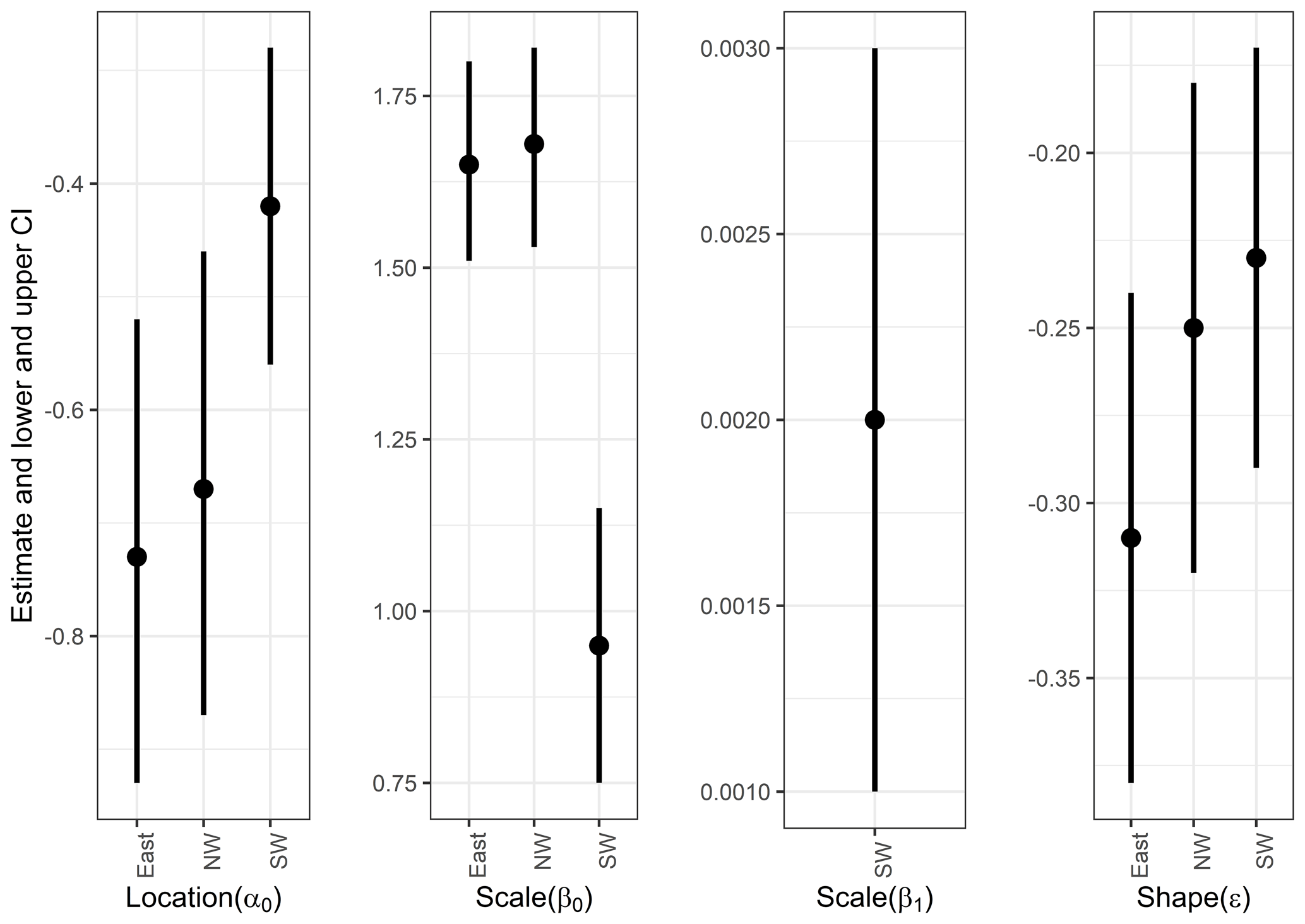
Figure 4 The 95 % confidence intervals of parameters based on the normal approximation for each parameter. Also numerical values are listed in Table S1.

3.1.1 Fitting GEV distributions to the tree-ring-reconstructed PDSI for return period estimation

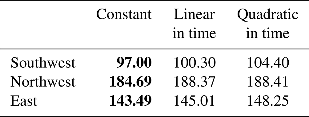
We construct two types of models: (1) stationary and nonstationary extreme value models and (2) nonstationary models using climatic variables as covariates. First, we consider polynomial models in time of the order of 0 to 2 for both the location and the scale parameters of the GEV distribution, resulting in seven models to be tested, including the stationary model, for each region. In addition, autoregressive (AR) models are examined. The models are evaluated based on the BIC (Table 3). The best GEV models and their maximum likelihood estimates (MLEs) with 95 % confidence intervals are as follows (Table 3, Fig. 4):

• Southwest. The estimated values of the model with a constant in the location parameter and temporally linear in the scale parameter and the AR(3) model's estimated values are

  $$\begin{array}{ll}{\displaystyle }& {\displaystyle }\mathit{\mu }=-\mathrm{0.42},\mathit{\sigma }=\exp (\mathrm{0.95}+\mathrm{0.002}t),\\ {\displaystyle }& {\displaystyle }\mathit{\epsilon }=-\mathrm{0.23}(\mathrm{BIC}=\mathrm{1045})\mathrm{and}\\ {\displaystyle }& {\displaystyle }\mathit{\mu }=-\mathrm{0.39}+\mathrm{0.36}{\mathrm{PDSI}}_{t-\mathrm{3}},\mathit{\sigma }=\mathrm{1.19},\\ {\displaystyle }& {\displaystyle }\mathit{\epsilon }=-\mathrm{0.29}(\mathrm{BIC}=\mathrm{1005}).\end{array}$$

• Northwest. The estimated values of the model with a constant in both the location and the scale parameters and the AR(3) model's estimated values are

  $$\begin{array}{ll}{\displaystyle }& {\displaystyle }\mathit{\mu }=-\mathrm{0.67},\mathit{\sigma }=\mathrm{1.68},\mathit{\epsilon }=-\mathrm{0.25}(\mathrm{BIC}=\mathrm{1241})\mathrm{and}\\ {\displaystyle }& {\displaystyle }\mathit{\mu }=-\mathrm{0.57}+\mathrm{0.50}{\mathrm{PDSI}}_{t-\mathrm{3}},\mathit{\sigma }=\mathrm{1.47},\\ {\displaystyle }& {\displaystyle }\mathit{\epsilon }=-\mathrm{0.27}(\mathrm{BIC}=\mathrm{1146}).\end{array}$$

• East. The estimated values of the model with a constant in both the location and the scale parameters and the AR(1) model's estimated values are

  $$\begin{array}{ll}{\displaystyle }& {\displaystyle }\mathit{\mu }=-\mathrm{0.93},\mathit{\sigma }=\mathrm{1.65},\mathit{\epsilon }=-\mathrm{0.31}(\mathrm{BIC}=\mathrm{1212})\mathrm{and}\\ {\displaystyle }& {\displaystyle }\mathit{\mu }=-\mathrm{0.55}+\mathrm{0.62}{\mathrm{PDSI}}_{t-\mathrm{1}},\mathit{\sigma }=\mathrm{1.25},\\ {\displaystyle }& {\displaystyle }\mathit{\epsilon }=-\mathrm{0.22}(\mathrm{BIC}=\mathrm{1064}).\end{array}$$

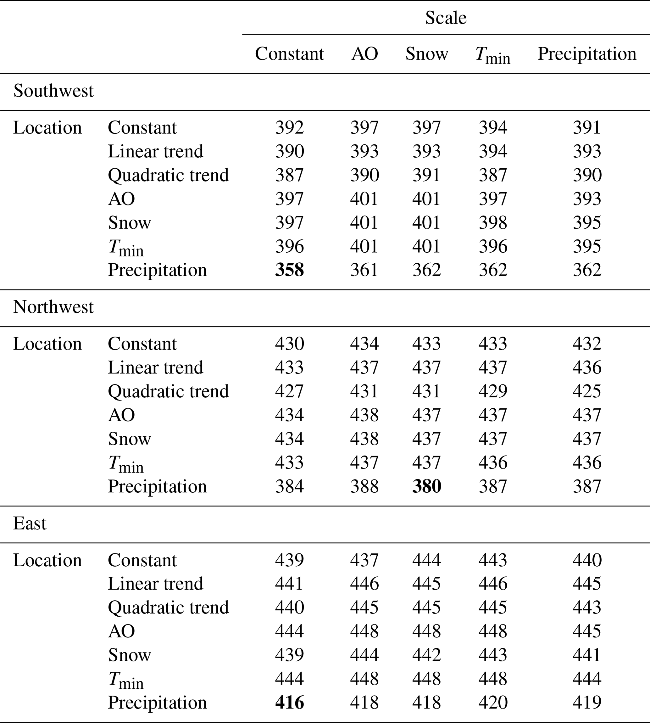
Table 3 BIC values for stationary and nonstationary GEV models fitted to the tree-ring-reconstructed PDSI values.

Note that L stands for the location parameters, S stands for the scale parameters, 0 means a constant in the parameter, 1 is temporally linear, and 2 is temporally quadratic for each parameter. Bold BIC values mean the lowest values.

These results suggest that in the long run, a stationary model for the PDSI in Mongolia may be appropriate. Only the southwest has nonstationarity in the scale parameter. This nonstationarity in the scale parameter for the southwest, with a mean coefficient of 0.002 relative to the constant value of 0.95, means that over 100 years the variability could increase from 0.9 to 1.05. If we take 0.9 to be a mid-period estimate, this would be rather a modest change. This could be a real feature or an artifact of the non-constant reconstruction variance from the tree-ring reconstruction algorithm.

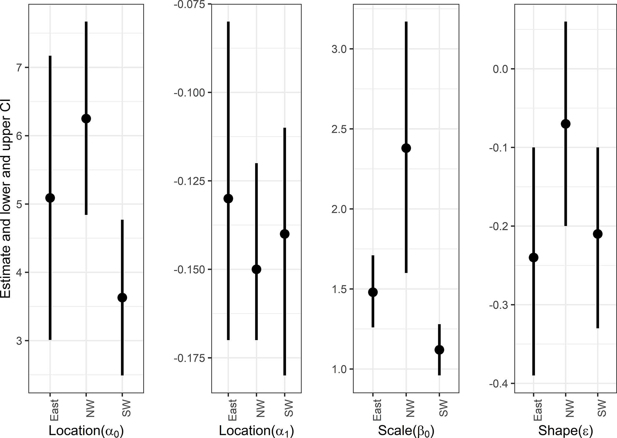
Figure 5 The 95 % confidence intervals of parameters, using other climate variables based on the normal approximation. Also numerical values are listed in Table S2.

Next, we estimate parameters of the GEV distribution functions fitted to the PDSI values by including other climate variables, such as the AO index, summer precipitation, snow, and minimum temperatures, as covariates from 1903 to 2010. Summer precipitation is a mean of May to August of the previous year, while snow is a mean of values from November of the previous year to the following February. Also, AO index data start in 1903. Thus, we use data starting in 1903 though the data themselves exist from 1901. The minimum temperature is a minimum value from November of the previous year to the following October. The GEV models with the lowest BIC for each cluster and MLEs with 95 % confidence intervals are detailed below (Table 4 and Fig. 5).

• Southwest. Precipitation data are as a linear covariate in the location parameter as follows:

  $$\begin{array}{ll}{\displaystyle }& {\displaystyle }\mathit{\mu }=\mathrm{3.63}-\mathrm{0.14}\mathrm{precipitation};\mathit{\sigma }=\mathrm{1.12};\\ {\displaystyle }& {\displaystyle }\mathit{\epsilon }=-\mathrm{0.21}(\mathrm{BIC}=\mathrm{358}).\end{array}$$

• Northwest. Precipitation data are as a linear covariate in the location parameter, and snow data are as a linear covariate in the scale parameter as follows:

  $$\begin{array}{ll}{\displaystyle }& {\displaystyle }\mathit{\mu }=\mathrm{6.25}-\mathrm{0.15}\mathrm{precipitation};\mathit{\sigma }=\mathrm{2.38}-\mathrm{0.31}\mathrm{snow};\\ {\displaystyle }& {\displaystyle }\mathit{\epsilon }=-\mathrm{0.07}(\mathrm{BIC}=\mathrm{380}).\end{array}$$

• East. Precipitation data are as a linear covariate in the location parameter as follows:

  $$\begin{array}{ll}{\displaystyle }& {\displaystyle }\mathit{\mu }=\mathrm{5.09}-\mathrm{0.13}\mathrm{precipitation};\mathit{\sigma }=\mathrm{1.48};\\ {\displaystyle }& {\displaystyle }\mathit{\epsilon }=-\mathrm{0.24}(\mathrm{BIC}=\mathrm{380}).\end{array}$$

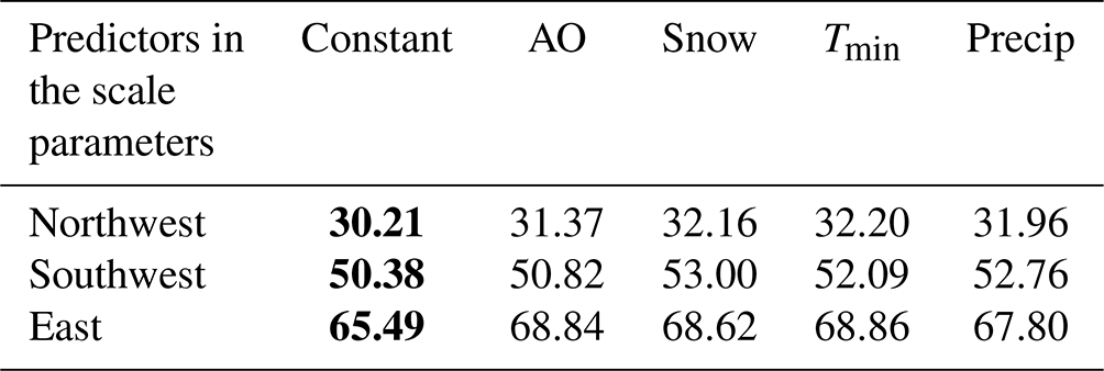
In the GEV models, climate variables (precipitation and snow) are important covariates for the extreme values of the PDSI values and improve the model performance (Table 3). These climate variables have no inter-year dependence that is significant based on ARIMA, and hence there is no memory in these variables and the best model is the stationary model. Consequently, no near-term forecast is feasible.

Table 4 BIC values in estimated GEV models fitted to the PDSI values using the climate variables from 1903 to 2010.

Note that bold BIC values mean the lowest values.

The time series of effective return periods of 100-year events for the GEV distribution functions fitted to the PDSI using the climate variables are shown in the southwest, northwest, and east from 1903 to 2010 (Fig. 6). This shows that variabilities in return periods of 100-year events of the PDSI values become larger over time in all the regions. Before 1940, the variabilities are small possibly because the instrumental data records began in the 1940s. Even after the 1940s, it also shows that the magnitude of 100-year events has increased in the last half of the data series. A PDSI value of 3 used to be a 100-year event in around 1920. Yet, at around the beginning of the 21st century, it had increased to be between 4 and 5. However, considerable inter-annual and decadal variability is evident.

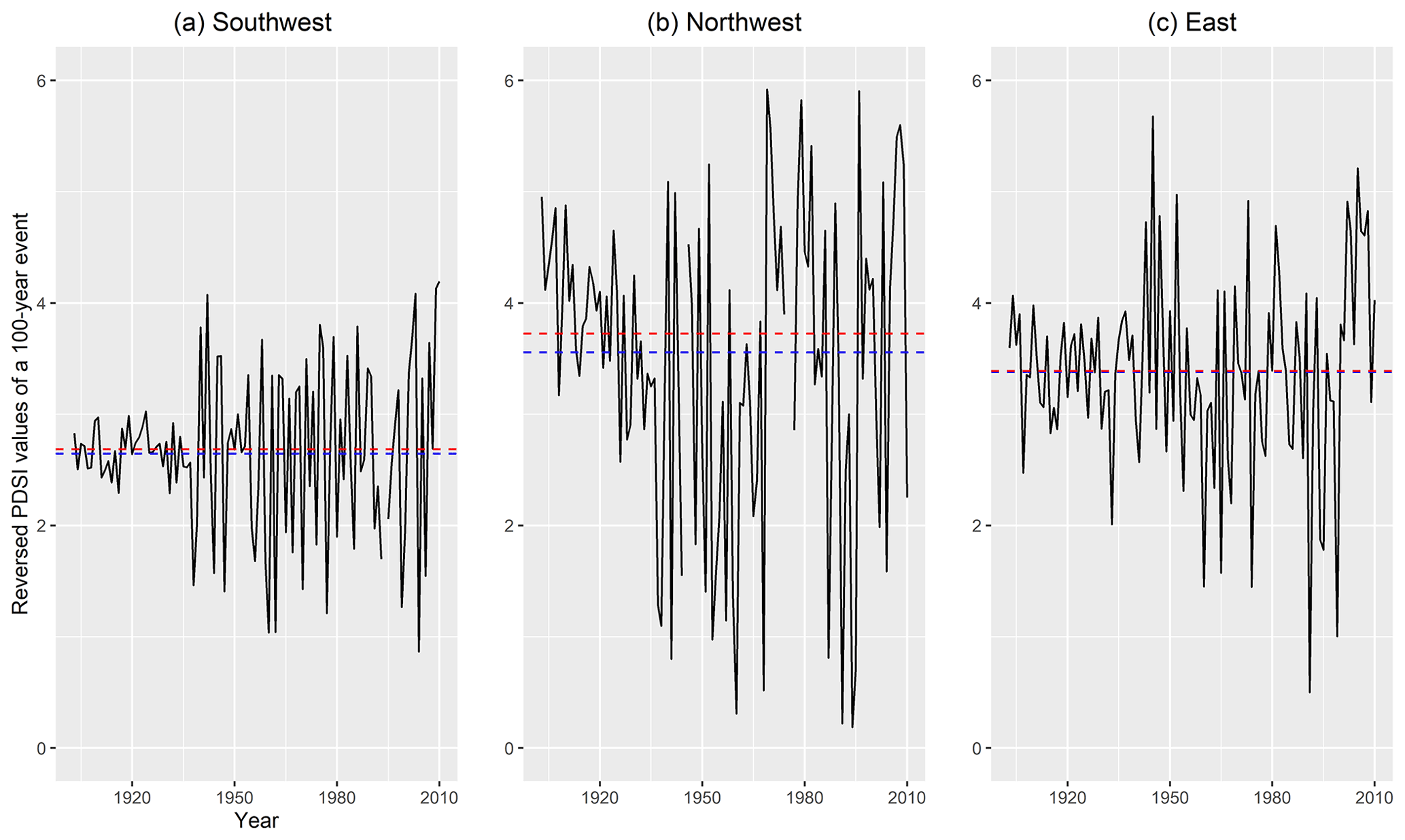
Figure 6 Estimated effective return periods of a 100-year event from the GEV distribution function fitted to the PDSI values in the southwest over 1903 to 2010 with precipitation data as a linear covariate in the location parameter. Variabilities in return periods of 100-year events of the PDSI values become larger over time in all the regions. The horizontal blue line is the mean of the effective return periods, while the red one is its median. Please note that the vertical axis is shown by the reversed values of PDSI values, meaning that a positive value is a drought condition.

The relationship between significant climate covariates and reversed reconstructed PDSI values based on the best GEV models for each return period of 10-, 50-, and 100-year events is shown in Figs. 7 and 8. The figures show that less precipitation leads to higher reversed reconstructed PDSI values, meaning more likelihood of droughts. Consequently, with this model, future projections of precipitation could be helpful to predict drought severity and frequency.

Figure 7 Relationship between precipitation and reversed reconstructed PDSI values in the southwest (a) and the east (b) based on the best GEV model. Since the PDSI values are reversed, the positive values mean drought conditions. The red, blue, and green lines are 10-, 50-, and 100-year events. This shows that less precipitation leads to higher reversed reconstructed PDSI values, meaning more likelihood of droughts.

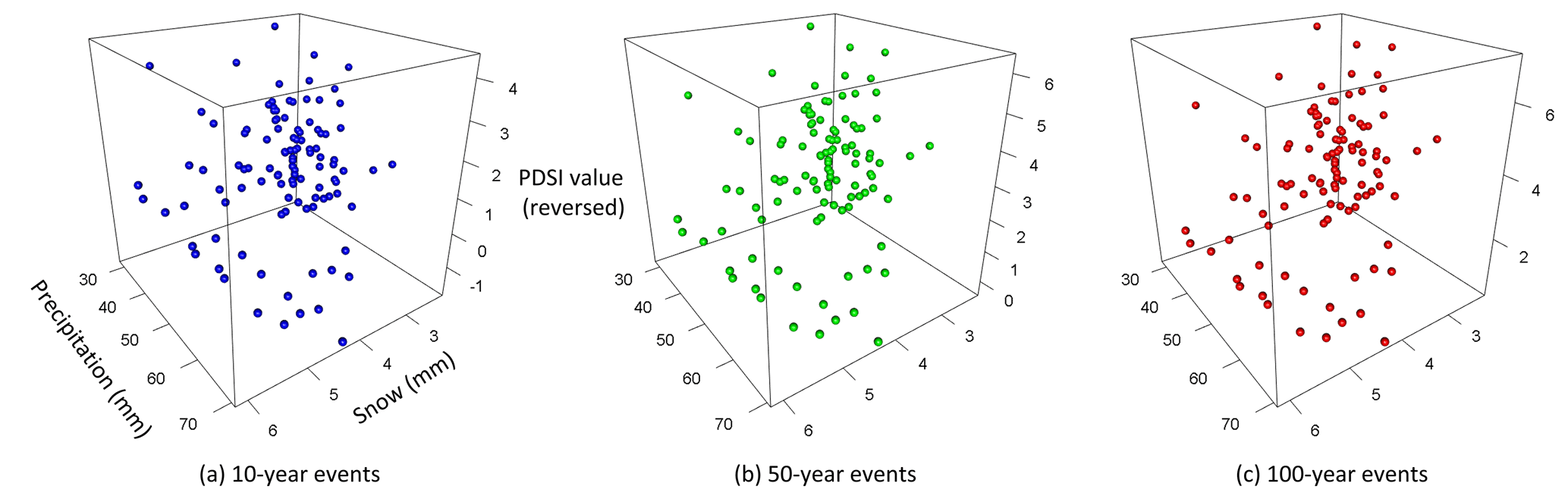
Figure 8 Relationship between precipitation, snow, and reversed reconstructed PDSI values in the northwest based on the best GEV model. Since the PDSI values are reversed, the positive values mean drought conditions. The x axis is precipitation; the y axis is snow; the z axis is reversed reconstructed PDSI values. The left cube (a) is for 10-year events, the central (b) is for 50-year events, and the right (c) is for 100-year events. Since the best GEV model contains precipitation and snow as covariates, the model for the northwest is cubic. This shows that less precipitation leads to higher reversed reconstructed PDSI values, meaning more likelihood of droughts.

3.1.2 Fitting GPDs to the tree-ring-reconstructed PDSI for the return period estimation

To fit a GPD, a threshold needs to be selected. We selected a threshold of 1.0 (please see Sect. S1 in the Supplement for a detailed explanation of how we chose the threshold). GPDs are fitted to the tree-ring-reconstructed PDSI values from 1700 CE as both stationary and nonstationary models (Table 5). The model of stationarity is best in terms of the BIC for all clusters.

Table 5 BIC values for nonstationary models in the scale parameters of GPD models fitted to the tree-ring-reconstructed PDSI from 1700 for each cluster.

Note that bold BIC values mean the lowest values.

The likelihood ratio test shows similar results. The likelihood ratio between temporal linear and stationary models shows that the p value is 0.24. The likelihood ratio test between temporal quadratic and stationarity models shows 0.49 in terms of p values. Both results show that the subset models do not improve significantly. These results confirm that for PDSI values a stationary model is appropriate.

Being similar to the GEV cases, we analyze the other climate variables after 1903. Table 6 shows that the best model of GPDs is the one with a constant in the scale parameters in terms of the BIC for all clusters. MLEs estimated by the best GPD models are shown in Fig. 9. The table shows that for catastrophic droughts, climate variables are not a significant covariate, although the differences in BIC values in the southwest and northwest between the ones with constants and with the AO index are small. The estimated effective return periods based on these best GPD models are listed in Table 7. In Table 7, the difference between the values for 10, 50, and 100 years is slight because the shape parameters estimated from the GEV for each case are negative. This means that the data are negatively skewed, and this leads to an implicit upper bound for the process. As a result, each of the quantiles is restricted by that upper bound, and they end up quite close to each other.

Table 6 BIC values for different GPD models fitted to the tree-ring-reconstructed PDSI values from 1903 with climate variables for all clusters.

Note that bold BIC values mean the lowest values.

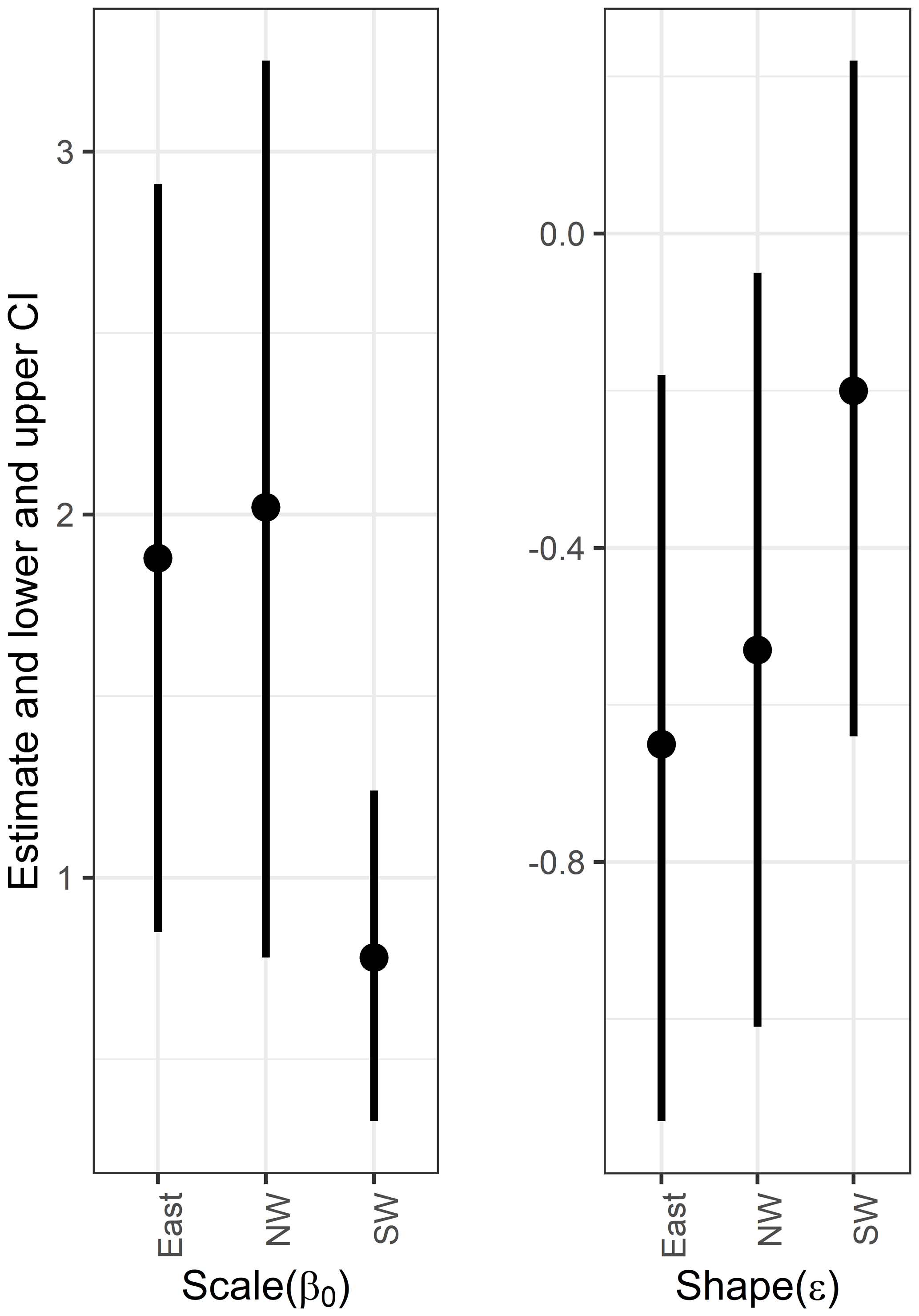
Figure 9 The 95 % confidence intervals of parameters, using other climate variables based on the normal approximation. Also numerical values are listed in Table S3.

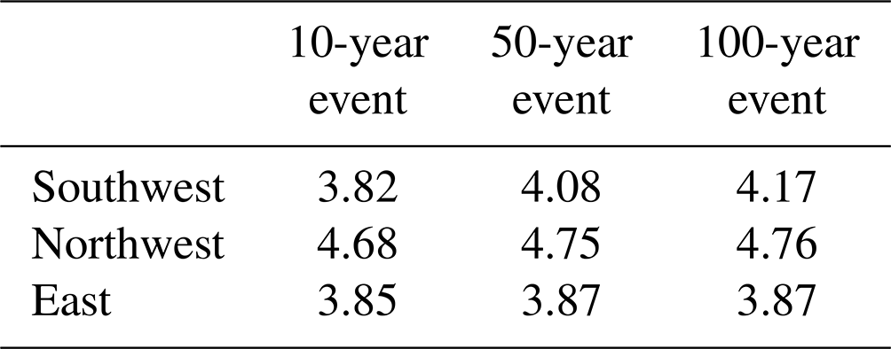
Table 7 Effective return periods of 10-, 50-, and 100-year events of the PDSI values, based on the best GPD models. (The actual PDSI values are negative ones of these values.)

3.1.3 Results based on GEV and GPD models

In this section, we fitted the GEV distribution function and GPD function to the PDSI values. Results are the following:

• The PDSI values will follow the distributions with ε<0, namely the Weibull distribution for the GEV models and the upper-bounded beta distribution for the GPD models. This information can be used to estimate return periods of extreme drought.

• For the southwest, the nonstationary models performed better if we look at GEV models without a threshold. However, with a threshold of 1 for the GPDs, the stationary models perform better than the nonstationary models, which indicates that all trends in reconstructed PDSI values are influenced by small events and not by extreme events; i.e., extreme events are stationary. For both the northwest and the east, stationary models performed better for both the GEV and the GPD models.

• Compared to the models with constants in the parameters, the GEV models with the climate variables are better in terms of the BIC value. Therefore, establishing a relationship between drought conditions and climate variables, particularly precipitation and snow, is useful in understanding the dynamics that determine dry conditions. However, compared to the models with constants in the scale parameters, the GPD models with the climate variables do not lead to improvement in the model performance in terms of the BIC.

• In terms of the BIC, the models of a GPD fitted to tree-ring-reconstructed PDSI values show better performance than the GEV models.

• Because of the third point, the effective return periods based on the GEV models change with the climate variables. In contrast, the effective return periods based on the GPD models are constant; for example, a 100-year event has the PDSI value of −4.17 for the southwest, −4.76 for the northwest, and −3.87 for the east. This suggests that while the magnitude of the annual maxima seems to change with the base climate conditions, the frequency of the extreme events beyond a threshold is not affected that much.

3.2 Simulating annual minimum temperature in Mongolia using Siberia data

Instrumental winter temperature data in Mongolia are limited before 1950. Also the gridded climate database that covers Mongolia starts after 1901. Thus, we attempt to estimate the Mongolia data from longer records from Siberia, which can go back to 1820. Existing studies suggest the winter temperatures between Mongolia and Siberia are correlated spatially, driven by polar jet dynamics (He et al., 2017; Iijima and Hori, 2018; Munkhjargal et al., 2020). First, winter temperatures in Mongolia will be simulated by using instrumental temperature data from Siberia (in Sect. 3.2). By using the simulated winter temperature in Mongolia, return periods of extreme cold temperature during winters will be estimated in Sect. 3.3.

The procedure was implemented as follows:

1. Conduct correlation analysis between Siberia and Mongolia data to select which station data are informative for temperature in Mongolia.

2. Impute missing data of instrumental data in Siberia.

3. Fit a GEV and GPD to the winter minimum temperature in Mongolia with the Siberia data.

4. Simulate the winter minimum temperature of Mongolia from Siberia data based on the best GEV model.

5. Calculate effective return periods of 10, 50, and 100 years from the simulated winter minimum temperature of Mongolia.

First, correlation analysis is conducted to see which station data in Siberia are useful for Mongolia data. Temperature data in both Mongolia and Siberia are monthly data. We use minimum temperature and average temperature during the wintertime (October to April) to remove the seasonality. We remove the seasonality because if both data series have seasonality (or periodicity), the correlation between them will be high just for that reason. Removing seasonality helps us identify if the anomalies from the periodic behavior are correlated or namely if they share similar dynamics in effects induced by atmospheric circulation beyond the seasonal cycle. Data are taken for the common periods when all the points have data (i.e., between 1901–1990). Irkutsk data alone are used since they alone show significant correlations between the temperature data in Mongolia and Siberia (results of Pearson and Spearman correlation coefficients and scatterplots are shown in Table S4 and Figs. S8 and S9, respectively). We also check the ACF of residuals between data from Irkutsk, Siberia, and winter average temperature of each cluster and find that there are no significant ACF structures between these data (Fig. S10).

Next, we checked the structures of missing data from Irkutsk. Some years are missing all monthly records. We impute Irkutsk's data with pattern-matching methods, which are equivalent to k-nearest neighbors, by Gibbs sampling using the predictive mean matching method (Van Buuren and Groothuis-Oudshoorn, 2011). Using winter minimum temperature from the Irkutsk data in Siberia ($T_{{\min }_{\mathrm{Irkutsk}}}$) as a covariate, we fit the Mongolia winter minimum temperature ($T_{{\min }_{\mathrm{mongolia}}}$) based on the GEV and GPD models.

3.2.1 Fitting GEV distributions to the winter minimum temperature in Mongolia

The results for GEV models based on the BIC are shown in Table 8. Models with Siberia data in both the location and the scale parameter have the lowest BIC for the northwest. For the southwest and east, the one with Siberia data in the location parameter and that is constant in the scale parameter shows the lowest BIC (Table 8). The best models for each region are shown in Fig. 10 and in the following:

$$\begin{array}{}\text{(6)}& {\displaystyle }& {\displaystyle }H\left(T_{{\min }_{\mathrm{mongolia}}}\right)=\mathrm{1}-{\left[\mathrm{1}+\mathit{\epsilon }\left({\displaystyle \frac{T_{{\min }_{\mathrm{mongolia}}}-\mathit{\mu }}{{\mathit{\sigma }}_{\mathit{\mu }}}}\right)\right]}_{+}^{-\mathrm{1}/\mathit{\epsilon }},\text{(7)}& {\displaystyle }& {\displaystyle }Zt\sim \mathrm{GEV}\left(\mathit{\mu }\right(t),\mathit{\sigma }(t),\mathit{\epsilon }(t\left)\right),\end{array}$$

where

$$\begin{array}{ll}{\displaystyle }& {\displaystyle }\mathit{\mu }\left(T_{{\min }_{\mathrm{Irkutsk}}}\right)={\mathit{\beta }}_{\mathrm{0}}+{\mathit{\beta }}_{\mathrm{1}}\cdot T_{{\min }_{\mathrm{Irkutsk}}};\\ {\displaystyle }& {\displaystyle }\mathit{\sigma }\left(T_{{\min }_{\mathrm{Irkutsk}}}\right)=\exp \left(\mathit{\beta }\mathrm{3}+{\mathit{\beta }}_{\mathrm{4}}\cdot T_{{\min }_{\mathrm{Irkutsk}}}\right);\\ {\displaystyle }& {\displaystyle }\mathit{\epsilon }\left(t\right)=\left\{\begin{array}{cl}{\mathit{\epsilon }}_{\mathrm{0}},& t\le t_{\mathrm{0}}\\ {\mathit{\epsilon }}_{\mathrm{1}},& t>t_{\mathrm{0}}\end{array};\right.\\ {\displaystyle }& {\displaystyle }\mathrm{for}\mathrm{the}\mathrm{southwest},\mathit{\mu }=\mathrm{11.80}+\mathrm{0.39}{T}_{{\min }_{\mathrm{Irkutsk}}},\mathit{\sigma }=\mathrm{1.90},\\ {\displaystyle }& {\displaystyle }\mathrm{and}\mathit{\epsilon }=-\mathrm{0.25};\\ {\displaystyle }& {\displaystyle }\mathrm{for}\mathrm{the}\mathrm{northwest},\mathit{\mu }=\mathrm{12.67}+\mathrm{0.52}{T}_{{\min }_{\mathrm{Irkutsk}}},\\ {\displaystyle }& {\displaystyle }\mathit{\sigma }=\exp \left(\mathrm{0.35}+\mathrm{0.06}{T}_{{\min }_{\mathrm{Irkutsk}}}\right),\\ {\displaystyle }& {\displaystyle }\mathrm{and}\mathit{\epsilon }=-\mathrm{0.18};\mathrm{and}\\ {\displaystyle }& {\displaystyle }\mathrm{for}\mathrm{the}\mathrm{east},\mathit{\mu }=\mathrm{10.20}+\mathrm{0.48}{T}_{{\min }_{\mathrm{Irkutsk}}},\mathit{\sigma }=\mathrm{1.40},\\ {\displaystyle }& {\displaystyle }\mathrm{and}\mathit{\epsilon }=-\mathrm{0.38}.\end{array}$$

Table 8 BIC values for GEV models using Irkutsk data for three clusters.

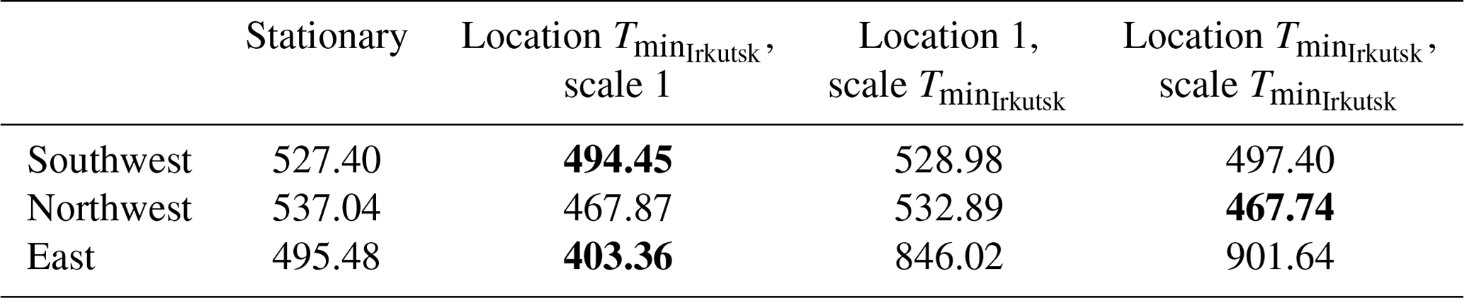
Note that bold BIC values mean the lowest values.

Figure 10 The 95 % confidence intervals of estimated parameters based on the best GEV model fitted to the winter minimum temperature in three clusters using Irkutsk data. Numerical values are listed in Table S5.

3.2.2 Fitting GPDs to the winter minimum temperature in Mongolia

For GPDs, we select 23 ^∘C (−23 ^∘C in reality) as a threshold (please see Sect. S1 and Figs. S6 and S7 regarding how the thresholds were selected). In this case, the model with Irkutsk's data in the scale parameter has the lowest BICs for all clusters as Table 9 shows. The best models for each cluster are shown in Fig. 11.

Table 9 BIC values of GPD models using Irkutsk data for three clusters.

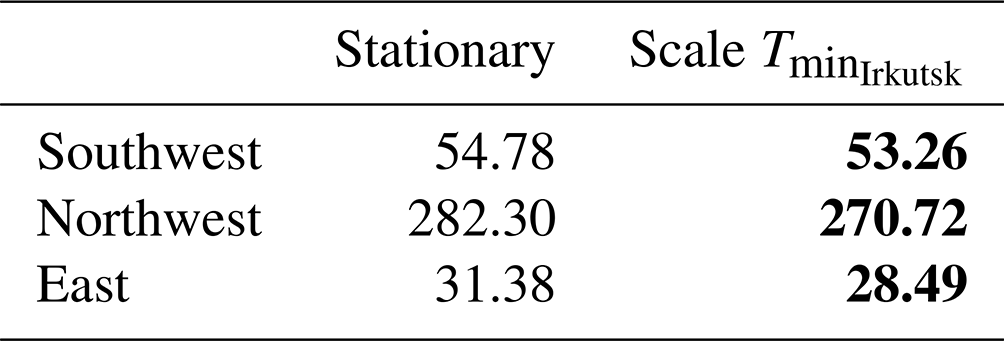
Note that bold BIC values mean the lowest values.

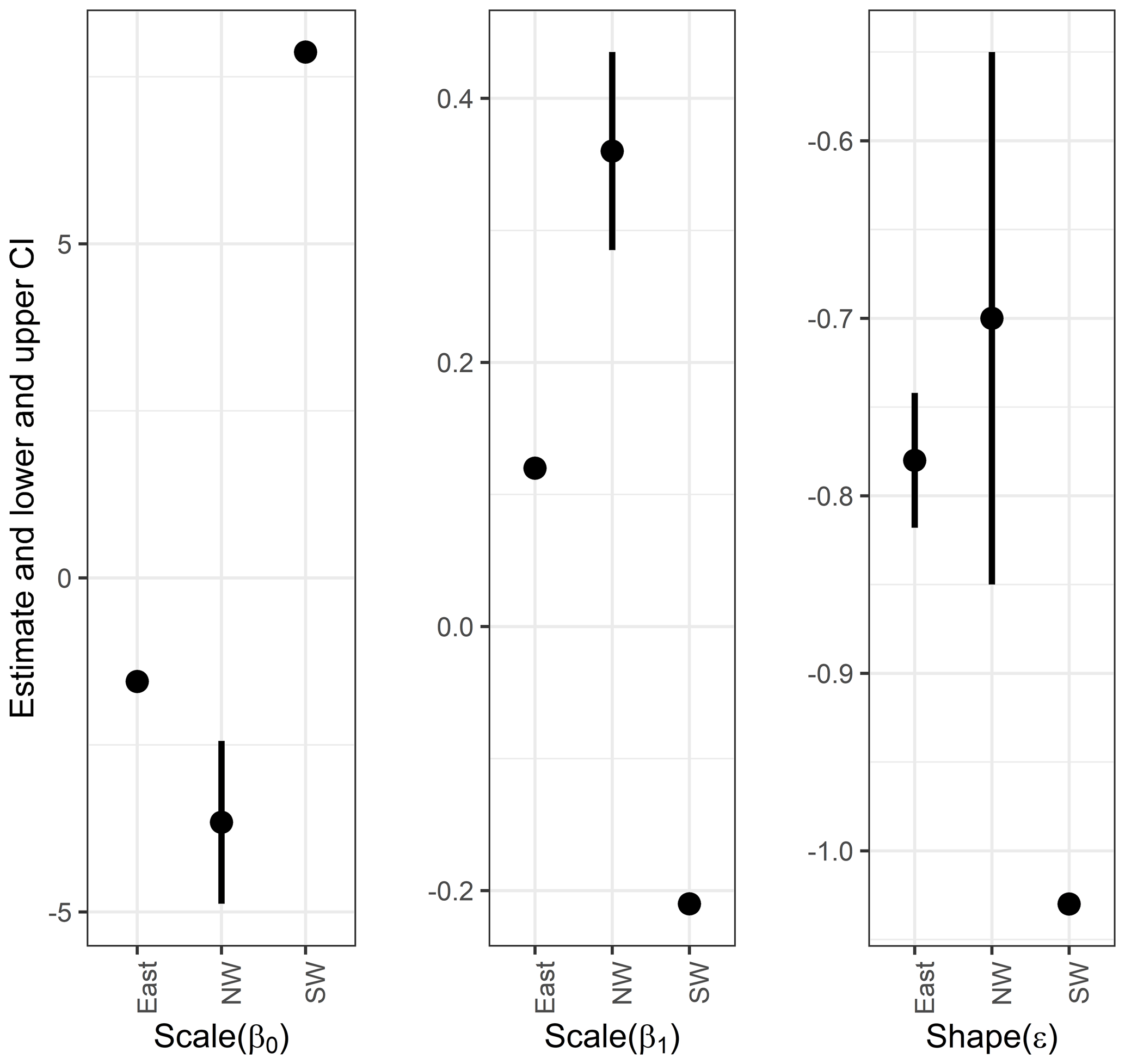
Figure 11 The 95 % confidence intervals of estimated parameters based on the best GPD model fitted to the winter minimum temperature in three clusters using Irkutsk data. Numerical values are listed in Table S6.

3.2.3 Results based on GEV and GPD models

In this section, we fitted the GEV distribution and GPD to the winter minimum temperature in Mongolia. The results are as follows:

• All the results show that the winter minimum temperature will follow the distributions with ε<0, namely the Weibull distribution for GEV models and the upper-bounded beta distribution.

• Based on BIC, GPD models show better performance in both the southwest and the east regions, while the GED models show better performance in the northwest.

3.3 Return periods of the winter minimum temperature in Mongolia simulated from Siberia data

Next, we simulate the Mongolia winter minimum temperature based on data from Irkutsk, Siberia, for 197 years using the parameters estimated by the best GEV model. Then, using these simulated Mongolia winter minimum temperatures, we estimate the 90% confidence intervals of return periods of 10-, 50-, and 100-year events for each cluster (Fig. 12). The medians of 100-year return periods are −26.08, −27.99, and −25.31 ^∘C for the southwest, northwest, and east. The variations in these density plots come from both the statistical properties of the Mongolia data themselves and variations attributed to Siberia data.

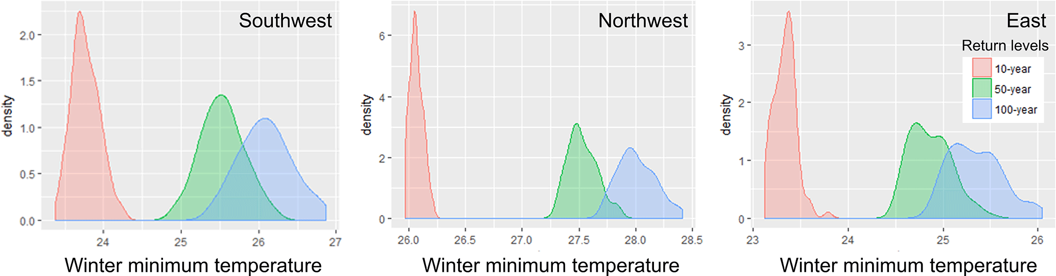
Figure 12 Density plots of 10-, 50-, and 100-year return periods of the winter minimum temperatures in the southwest, northwest, and east of Mongolia with 90 % confidence intervals. Please note that the x axis shows temperature below zero (i.e., for the southwest, the axis shows negative 23.5 to 27 ^∘C). The data are simulated 100 times from the Siberia data. For example, the plots show that the medians of 100-year return periods are −26.08, −27.99, and −25.31 ^∘C for the southwest, northwest, and east.

4 Binary index of the co-occurrence of summer drought and cold winter temperatures

Based on the thresholds used in the GPD approaches, we also explored if the frequency of the co-occurrence of summer drought and cold winter temperatures has changed over time. First, we counted cases as a binary value of 1 when both summer drought and cold winter temperatures in Mongolia are below thresholds (−1 for PDSI values and −23 ^∘C for winter temperatures); otherwise we used zero. Then, we fitted the local binomial and Poisson regressions while computing generalized cross-validation statistics to determine the smoothing parameter (Loader, 2006) (please see Sect. S2 for α values used for each cluster). Figure 13 shows the northwest and east have similar long-term trends: decreasing trends in the early 20th century and slightly increasing trends since the 1990s. The southwest shows an increase in the mid-20th century, and this has started happening again in the early 21st century.

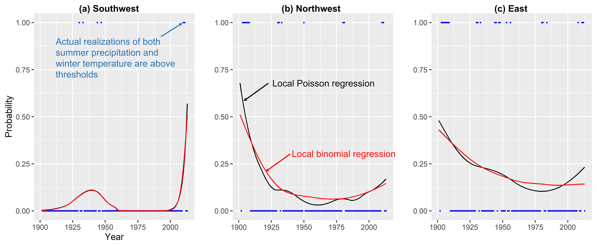
Figure 13 Binary index for the co-occurrence of threshold exceedance of PDSI values and winter temperature. The local regression is based on the optimal bandwidth of a local quadratic regression function based on the generalized cross-validation criteria considering that the binary indicator is an outcome of a nonhomogeneous Poisson process. Note the tendency for a cluster in the beginning for the northwest and the east. The increase in the frequency for the trend function in the most recent period could represent more of an edge effect of the regression.

5 Conclusions

Meteorological data in Mongolia are limited in length and have many missing values. Therefore, we utilize longer records from paleoclimate proxy data and meteorological data from neighboring Siberia. The motivation was to improve risk estimation for dzud in Mongolia. Based on extreme value theory, this study derived fitted distributions for drought and winter extreme cold conditions. The study also improved the estimation of return periods of extreme drought conditions and winter temperature, using the tree-ring-reconstructed self-calibrated PDSI and station records from Mongolia and Siberia.

GEV models without a threshold show that there is a trend in tree-ring-reconstructed PDSI data in the southwest, while there is a no trend in the PDSI in both the northwest and the east. However, the threshold approach indicates that extreme events in reconstructed PDSI values are stationary, in turn indicating that catastrophic drought conditions have been stationary for the last 300 years.

The study estimated the extreme distributions of drought and winter minimum temperatures in Mongolia. The PDSI values follow the distributions with ε<0, namely the Weibull distribution for the GEV models and the upper-bounded beta distribution for the GPD models. Also, the results of the study show that the winter minimum temperature follows the distributions with ε<0, namely the Weibull distribution for GEV models and the upper-bounded beta distribution. These estimated distributions can be used to improve the risk calculations for livestock index insurance in Mongolia.

Based on the results of our GEV model fitted to the PDSI values, we show that climate variables, such as precipitation and snow, are important covariates for the extreme values of the reconstructed PDSI values. However, for catastrophic drought events, climate variables are not significant covariates based on the results of the GPD model fitted to the PDSI values.

The GEV model also shows that the return periods of drought conditions are changing over time and variability is increasing for all the regions. Yet, based on GPDs, the return periods of drought conditions are constant: for example, the actual values of the PDSI for the 100-year events are −4.17 for the southwest, −4.76 for the northwest, and −3.87 for the east. The median of 100-year return periods of the winter minimum temperature in Mongolia is −26.08 ^∘C for the southwest, −27.99 ^∘C for the northwest, and −25.31 ^∘C for the east.

This study improves the return period estimation of droughts and winter minimum temperature. Summer drought and winter temperature are important predictors for livestock mortality since they explain 48.4 % of the total variability in the mortality data, along with summer precipitation and summer potential evapotranspiration (Rao et al., 2015). Therefore, this long-term estimation of return periods of these significant predictors can be used to improve risk analysis of high livestock mortality in order to prepare for the winter catastrophes through early warning systems and index insurance.

A binary index for the co-occurrence of threshold exceedance of drought severity and temperature was developed and its temporal variation assessed. The index shows that all the regions have had increasing trends of this co-occurrence since around 2000. Begzsuren et al. (2004) identify that mortality rates are higher in combined drought and dzud years than in those with dzud or drought alone while examining the co-occurrence of these extreme events with 51 years of observational data. This implies that the increasing trends of the co-occurrence would have severe socioeconomic impacts on the country's livestock industry.

Our study estimates the return intervals and underlying probabilistic characteristics of the climate variables. Index insurance requires a proper threshold and the understanding of underlying distributions of risk events (Haraguchi, 2018). Thus, the estimation of extreme value distributions and return periods has the potential to improve livestock index insurance, which is implemented in Mongolia by the government of Mongolia with the help of the World Bank (Mahul et al., 2015). Insurance is priced by considering the uncertainty associated with the estimation of the probability of exceeding the threshold at which the payout occurs. The estimation of the uncertainty is reduced as the length of record (in our case from the paleoclimate extension) increases. At present, no one in the industry is using paleoclimatic information to extend and reduce coverage costs, but there is interest in using it to understand the clustering of payouts. Furthermore, the results of this study increase understanding of how extreme climatic events in arid regions, which are sensitive to anthropogenic climate change, are changing. Given that some research projects increases in droughts in Mongolia (e.g., Bell et al., 2013; Li et al., 2020), the urgent need to build resilience to winter disaster and dzud is even more unequivocal.