Characterizing multivariate coastal flooding events in a semi-arid region: the implications of copula choice, sampling, and infrastructure

Multivariate coastal flooding is characterized by multiple flooding pathways (i.e., high offshore water levels, streamflow, energetic waves, precipitation) acting concurrently. This study explores the joint risks caused by the co-occurrence of high marine water levels and precipitation in a highly urbanized semi-arid, tidally dominated region. A novel structural function developed from the multivariate analysis is proposed to consider the implications of flood control infrastructure in multivariate coastal flood risk assessments. Univariate statistics are analyzed for individual sites and events. Conditional and joint probabilities are developed using a range of copulas, sampling methods, and hazard scenarios. The Nelsen, BB1, BB5, and Roch–Alegre were selected based on a Cramér–von Mises test and generally produced robust results across a range of sampling methods. The impacts of sampling are considered using annual maximum, annual coinciding, wet-season monthly maximum, and wet-season monthly coinciding sampling. Although annual maximum sampling is commonly used for characterizing multivariate events, this work suggests annual maximum sampling may substantially underestimate marine water levels for extreme events. Water level and precipitation combinations from wet-season monthly coinciding sampling benefit from a dramatic increase in data pairs and provide a range of physically realistic pairs. Wet-season monthly coinciding sampling may provide a more accurate multivariate flooding risk characterization for long return periods in semi-arid regions. Univariate, conditional, and bivariate results emphasize the importance of proper event definition as this significantly influences the associated event risks.

1 Introduction

Coastal flooding is a significant human hazard (Leonard et al., 2014; Wahl et al., 2015) and is considered a primary health hazard by the US Global Change Research Program (Bell et al., 2016). Coastal migration and utilization continues to increase (Nicholls et al., 2007; Nicholls, 2011). Over 600 million people populate coastal zones (Merkens et al., 2016). Climate-change-induced sea level rise will substantially increase flood risk (Church et al., 2013; Horton et al., 2014) and negatively impact coastal populations (Bell et al., 2016). Even relatively modest sea level rise will significantly increase flood frequencies through the US (e.g., Tebaldi et al., 2012; Taherkhani et al., 2020). Southern California is particularly vulnerable to sea level rise. Small changes in sea level (∼ 5 cm) double the odds of the 50-year flooding event (Taherkhani et al., 2020), and the 100-year event is expected to become annual by 2050 (Tebaldi et al., 2012). Regional research has explored flood risks caused by sea level rise and coastal forcing (e.g., Heberger et al., 2011; Hanson et al., 2011; Gallien et al., 2015). However, accurately characterizing future, non-stationary coastal vulnerability requires considering the joint and potentially nonlinear impacts of compound (marine and hydrologic) events (Gallien et al., 2018).

Compound coastal flooding considers the combined impacts of marine and hydrologic forcings, typically within a physically relevant time window, and are considered multivariate events. Typical events, such as precipitation or high water levels, occurring simultaneously may combine to generate extreme events (Seneviratne et al., 2012). In urban coastal settings multiple flooding pathways (i.e., high marine water levels, wave run-up and overtopping, large fluvial flows, and pluvial flooding from precipitation) interact with infrastructure (e.g., sea walls, human-made dunes, and the storm system), potentially exacerbating hazards. Notably, multivariate events that share a common return period may produce vastly different flooding outcomes. Traditionally, the literature has focused on river-discharge- or storm-surge-dominated multivariate events (Table 1).

From a flood risk perspective there are multiple methods to characterize events. A univariate approach is often used where a single variable (e.g., water level) is considered. For example, the Federal Emergency Management Agency (FEMA) recommends characterizing multivariate events by developing univariate water level and discharge statistics and then adopting a smooth, blended result for transitional areas (FEMA, 2011, 2016c). This can lead to underestimating flood risk because of the interplay between two flood pathways (i.e., a high tailwater forces fluvial flooding upstream). Conditional probabilities represent an alternative where the multivariate flood risk can be evaluated given available information on a primary variable (e.g., water level) to determine the exceedance probability of a secondary variable (e.g., precipitation) (Shiau, 2003; Karmakar and Simonovic, 2009; Zhang and Singh, 2012; Li et al., 2013; Mitková and Halmová, 2014; Serinaldi, 2015, 2016; Anandalekshmi et al., 2019). A third method uses copulas to analyze the dependence of multiple flood drivers and develop joint statistics.

Numerous studies have used a copula-based approach to study floods manifested by various combinations of variables (Table 1). Multivariate flood risks can be described and quantified from previous copula studies (Salvadori, 2004; Salvadori and De Michele, 2004, 2007; Salvadori et al., 2011, 2013, 2016). Multivariate inland and coastal hydrology analysis have primarily focused on a small group of copulas: Archimedean (Clayton, Frank, and Gumbel), Student t, and Gaussian copulas. Alternative copulas may more accurately characterize urban coastal flooding (Jane et al., 2020). Specifically, hazard scenarios provide various perspectives on critical multivariate events (Salvadori et al., 2016). Initial studies were primarily focused on select hazard scenarios (Table 1 in Salvadori et al., 2016).

Data sampling methods in multivariate studies influence distribution fitting. Two primary sampling methods exist: peaks over threshold (Jarušková and Hanek, 2006) and block maxima (Engeland et al., 2004). Events selected using peaks over threshold sampling are above a predetermined threshold defining an “extreme” event. Block maxima sampling uses various block sizes (yearly, seasonal, semiannual, etc.) to separate and select the maximum event per block. Engeland et al. (2004) report a significantly different 1000-year streamflow when using 12-month block sampling (160 m³s⁻¹) compared to using a threshold of 50 m³ s⁻¹ (120 m³ s⁻¹). Many studies utilize block maxima sampling with a yearly block size, i.e., the annual maximum sampling method (Baratti et al., 2012; Bezak et al., 2014; Wahl et al., 2015). This method is specifically recommended by FEMA (2016c) for evaluating coastal hazards. Alternatively, studies identify extremes in the primary variable using annual maximum sampling and select a secondary variable which co-occurs with the primary variable (Lian et al., 2013; Xu et al., 2014; Tu et al., 2018), creating a “coinciding”-type sampling. Multivariate applications relying upon annual maximum sampling generate events with severe flooding potentials which may produce unrealistic variable combinations. Coinciding sampling draws from physically realistic event pairs. Although, multiple studies explore sampling effects on fitted distribution parameters and univariate return periods (Engeland et al., 2004; Jarušková and Hanek, 2006; Peng et al., 2019; Juma et al., 2020), sampling effects for multivariate coastal flooding events are unknown.

Coastal flooding studies primarily focus on locations defined by storm-surge-dominated oceanographic conditions with warm, humid (Wahl et al., 2012; Lian et al., 2013; Xu et al., 2014; Masina et al., 2015; Wahl et al., 2015; Mazas and Hamm, 2017; Paprotny et al., 2018; Tu et al., 2018; Bevacqua et al., 2019; Didier et al., 2019; Xu et al., 2019; Yang et al., 2020), and monsoonal (Jane et al., 2020) climatic conditions (i.e., Köppen-Geiger system, Beck et al., 2018). In contrast, along the southern California coast typical tidal variability is 1.7 to 2.2 m (Flick, 2016), and storm surge rarely exceeds ∼ 20 cm (Flick, 1998). Notably, during the wet season (October to March), when precipitation typically occurs, spring tide ranges are relatively large (∼ 2.6 m). Critically, few studies consider areas where coastal flooding events are dominated by large tides and either precipitation or wave events (Masina et al., 2015; Mazas and Hamm, 2017; Didier et al., 2019; Jane et al., 2020). This study explores univariate and multivariate flooding events in a semi-arid, tidally dominated, highly urbanized region. Here, the dependency between observed water levels and precipitation, impacts of sampling methods and distribution fitting, and the resulting flood values are explored.

Masina et al. (2015); Mazas and Hamm (2017); Didier et al. (2019)De Michele et al. (2007); Salvadori et al. (2014, 2015)Wahl et al. (2012); Paprotny et al. (2018)White (2007); Bray and McCuen (2014); Sadegh et al. (2018); Ganguli and Merz (2019a, b)Paprotny et al. (2018); Ganguli et al. (2020)Yue (2001a, b); Shiau (2003); Favre et al. (2004); De Michele et al. (2005); Poulin et al. (2007); Li et al. (2013); Salvadori et al. (2013); Requena et al. (2013); Aghakouchak (2014)Bray and McCuen (2014); Jeong et al. (2014)Salvadori and De Michele (2010)Lian et al. (2013)Xu et al. (2014)Tu et al. (2018)Xu et al. (2019)Bevacqua et al. (2020)Yang et al. (2020)Jane et al. (2020)Wahl et al. (2015); Paprotny et al. (2018); Bevacqua et al. (2019)Yue (2000a, b, 2002); De Michele and Salvadori (2003)Anandalekshmi et al. (2019)Zhang and Singh (2012); Hao and Singh (2020)Zhong et al. (2020)Zhang et al. (2017)Salvadori and De Michele (2007)Zheng et al. (2014)Karmakar and Simonovic (2009); Reddy and Ganguli (2012); Ganguli and Reddy (2013); Gräler et al. (2013); Mitková and Halmová (2014)

Table 1 A non-exhaustive list of multivariate studies which utilized copulas to study the associated variables.

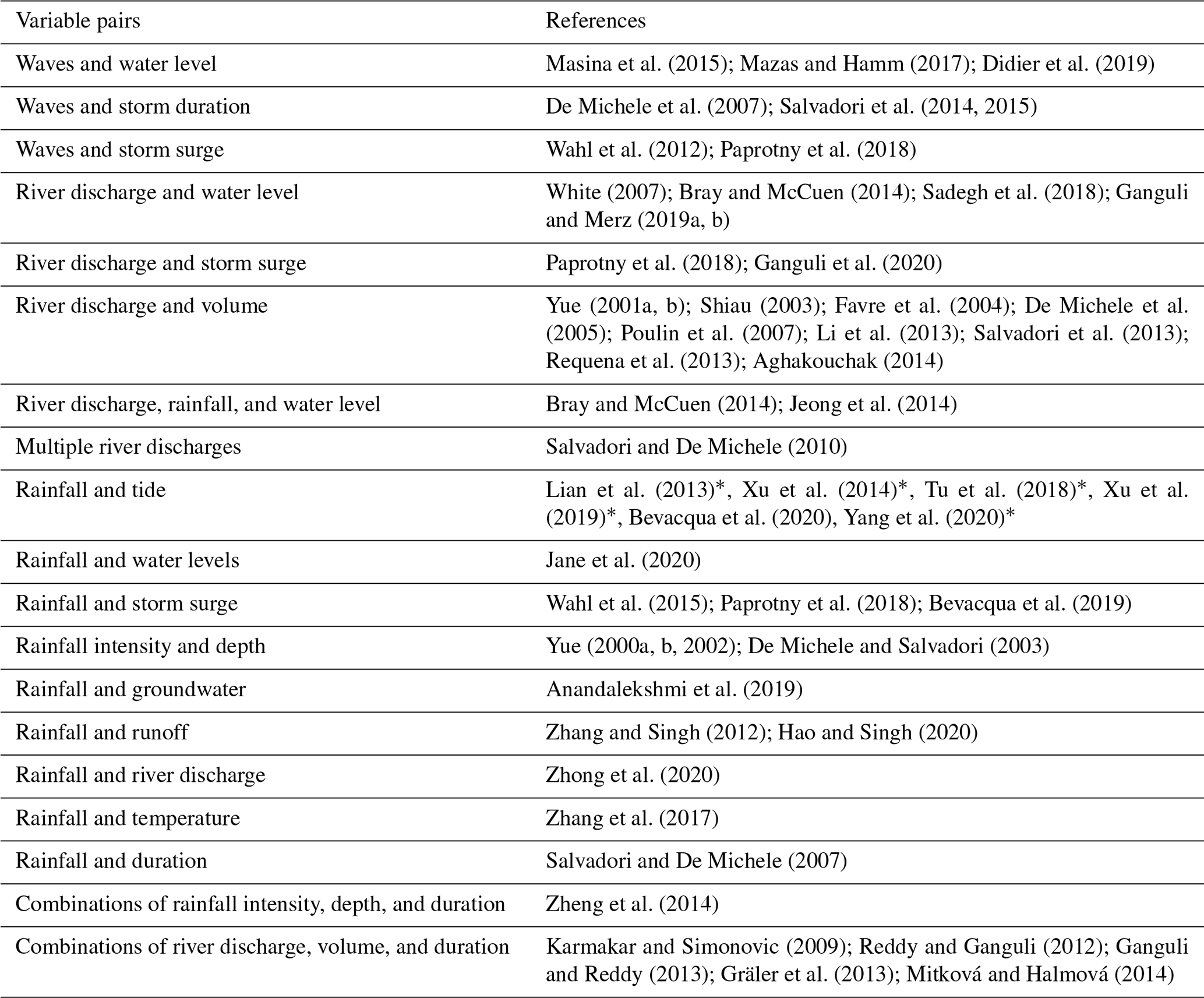
^* Note that these studies use the term tide measurement but actually represent observed water level measurements. Please refer to Sect. 2 for clarification.

2 Site description and data

This study considers observed water level and precipitation influences for coastal multivariate events at Santa Monica (SM), Sunset Beach (S), and LA Jolla (SD) areas in Los Angeles, Huntington Beach, and San Diego, California (Fig. 1): three semi-arid, tidally dominated sites in the United States. All are low-lying estuarine or bay-backed highly urbanized beach communities requiring extensive coastal management to mitigate flooding events. For example, sea walls and artificial berms in Sunset Beach protect infrastructure from high embayment water levels, wave run-up, and overtopping along the open coast. The storm drain network is managed to prevent back-flooding during high tides. Notably, Gallien et al. (2014) suggested that when tide valves are closed, the storm drain network cannot reduce pluvial flooding caused by alternative flooding pathways (e.g., precipitation or wave overtopping). The Pacific Coast Highway (PCH) is heavily utilized and is a primary transportation corridor along the southern California coastline. All locations are densely urbanized and highly impacted by flooding.

Observed water levels from the Los Angeles (station ID: 9410660), La Jolla (station ID: 9410230), and Santa Monica (station ID: 9410840) tide gauges are available on NOAA's Tides and Currents for daily high–low, hourly, or 6 min intervals (NOAA, 2021d). Verified hourly water levels (m NAVD88) had the longest record length at all three stations and provided an additional 31 years of observations overlapping precipitation data for Los Angeles and La Jolla, and 6 years for Santa Monica. The resulting observations windows are 22 November 1973 to 19 December 2013 for Santa Monica, 1 July 1948 to 1 December 2012 for Sunset, and 1 July 1948 to 19 December 2013 for San Diego (Table 2). It is worth noting that within the body of multivariate flooding literature, the terms tide and water level may be interchanged (e.g., Lian et al., 2013; Xu et al., 2014; Tu et al., 2018; Xu et al., 2019; Yang et al., 2020). This is a key distinction since compound event dependencies may change depending on water level selection. Recent efforts have been made to standardize language where tide represents only the astronomical changes in water levels and storm surge specifically excludes astronomical variability and consists only of the inverse barometric effects along with wind and wave setup (Gregory et al., 2019). In this study, the term observed water level (OWL) is adopted. OWL is the water level measured at the NOAA tide gauges, which includes all tidal, storm, and climatic effects.

The US Hourly Precipitation Data dataset provided by the NOAA's National Centers for Environmental Information (NOAA, 2021c) at the Signal Hill (COOP:048230), Los Angeles International Airport (COOP:045114), and San Diego International Airport (COOP:047740) stations is used as the precipitation inputs. Observations do not contain trace amounts (< 0.25 mm) and are provided as cumulative precipitation (mm) per event. Precipitation measurements were converted to a millimeters-per-hour rate by dividing the total event precipitation by the event duration to match the hourly OWL measurements. The final precipitation input is a 24 h cumulative precipitation record made from the hourly observations. All data were transformed to UTC for analysis.

Multivariate flood probabilities are determined with combinations of sampling methods: annual maximum (AM), annual coinciding (AC), wet-season monthly maximum (WMM), and wet-season monthly coinciding (WMC). AM sampling pairs the single largest precipitation and OWL observations within a given year (without regard to co-occurrence), where AC sampling pairs the single largest precipitation observation within a given year to the largest OWL observation within its 24 h accumulation period. Each sampling method samples from a unique probability space and therefore will provide varying perspectives for a return period. A summary of each sites' associated gauges, observation windows, and number of pairs is provided in Table 2. Southern California's wet season is defined between October to March and provides a majority of the total annual rainfall (Cayan and Roads, 1984; Conil and Hall, 2006). It is likely for extreme multivariate events to occur during this period. Maximum sampling pairs the single largest precipitation and OWL observations within each year or wet-season month. A multivariate event created with the largest observed precipitation and OWL within a year or wet-season month can result in an event with severe flooding potential. Although strictly speaking maximum parings (annual or wet season) do not technically represent an observed multivariate event, they would represent a severe event and are consistent with the blended approach recommended by FEMA (2016c). Coinciding sampling pairs the single largest precipitation observation within each year or wet-season month to the largest OWL observation within its 24 h accumulation period, providing more realistic pairs compared to maximum sampling.

Distributions are fit with existing precipitation observations greater than zero consistent with previous studies (Swift and Schreuder, 1981; Hanson and Vogel, 2008). Months with no OWL measurements were excluded. In the case of coinciding sampling, pairs that had three or more OWL measurements missing within the 24 h window were manually reviewed and removed if their tidal peak was clearly missing. Specifically for WMM sampling, months with more than half their observations missing were also reviewed and removed if the tidal peak was missing. The resulting data pairs are shown in Fig. 2.

Figure 1 Map displaying (a) Santa Monica, (b) Sunset, and (c) San Diego sites along with locations of tide gauges (triangle) and precipitation stations (circle). The road drain (square) and boundary (yellow) at Sunset (∼ 2 km²) are for the structural scenario. Aerial imagery from NOAA (2021a).

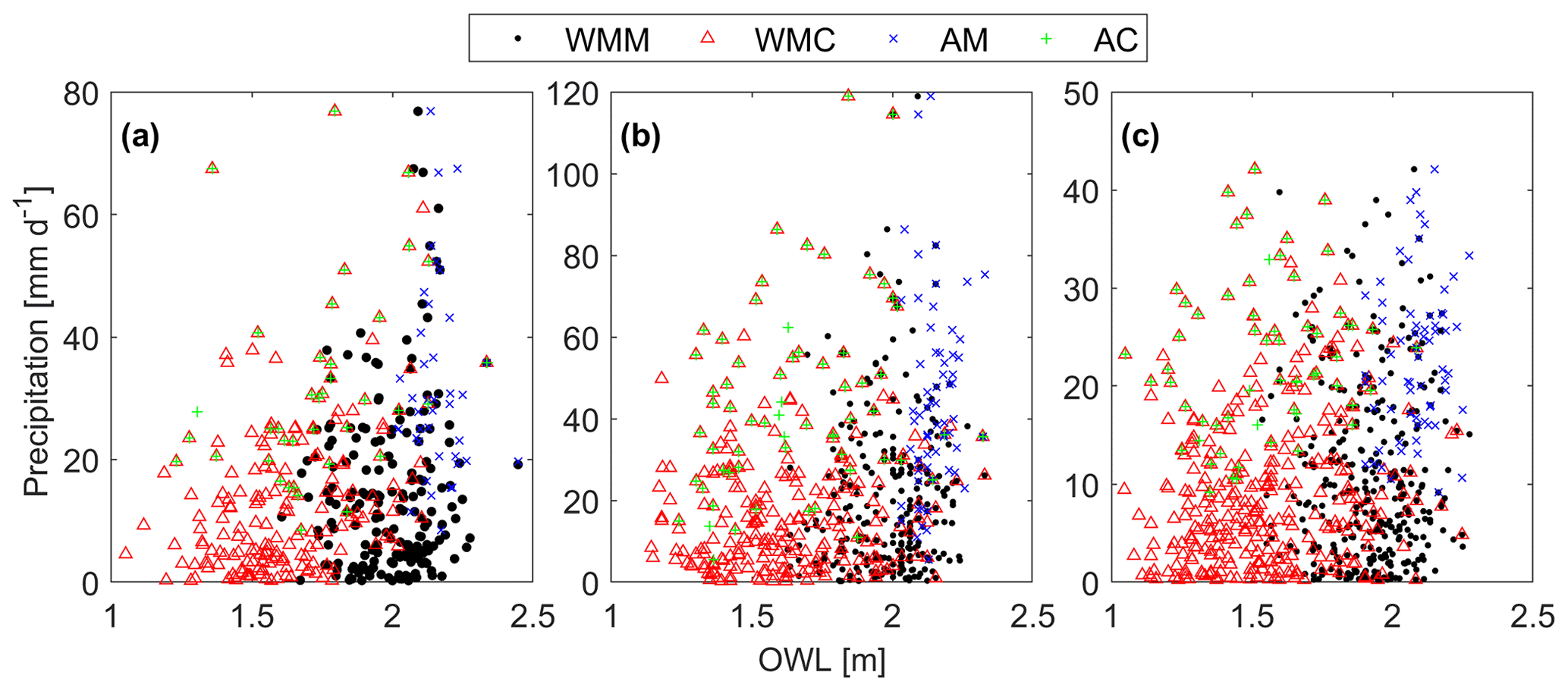
Figure 2 Data pairs for each sampling method. Annual maximum (AM; blue x), annual coinciding (AC; green +), wet-season monthly maximum (WMM; black ⋅), and wet-season monthly coinciding (WMC; red △) at (a) Santa Monica, (b) Sunset, and (c) San Diego.

Table 2 Water level and precipitation observations at Santa Monica (SM), Sunset (S), and San Diego (SD) using annual maximum (AM), annual coinciding (AC), wet-season monthly maximum (WMM), and wet-season monthly coinciding (WMC) samplings.

3 Methods

3.1 Univariate, bivariate, and conditional distributions

Potential flooding events are determined with three different probability definitions: univariate, conditional, and bivariate. Assuming X and Y are random variables, x and y are observations of these variables, and F_X and F_Y represent the variables' respective cumulative distribution functions (CDFs). Formulations for univariate (F_X(x),F_Y(y)) and bivariate joint (${\mathbf{F}}_{X,Y}(x,y)$) CDFs follow DeGroot and Schervish (2014) (Eqs. 1 and 2). Conditionals (${\mathit{F}}_{X|Y\ge y}\left(x\right|Y\ge y)$, ${\mathit{F}}_{X|Y\le y}\left(x\right|Y\le y)$, and ${\mathit{F}}_{X|Y=y}\left(x\right|Y=y)$) are developed from Shiau (2003) (Eq. 3) and Serinaldi (2015) (Eqs. 4 and 5). Conditionals 1 (C1), 2 (C2), and 3 (C3) represent Eqs. (3), (4), and (5) going forward. Univariate statistics are developed using the appropriate continuous random variable distribution, while conditional and bivariate CDFs are determined using copulas.

Copulas are functions that associate random variables' univariate CDFs with their joint CDF (e.g., F_X and F_Y with ${\mathbf{F}}_{X,Y}(x,y)$) according to Sklar's theorem (Sklar, 1959; Salvadori, 2004). There is no requirement for the univariate distributions to be the same. This is particularly advantageous since the optimal univariate distributions may be used for each variable. Bivariate probabilities for different hazard scenarios, which represent various multivariate events, and conditional probabilities can be calculated using fitted copula functions.

$$\begin{array}{}\text{(1)}& {\displaystyle }{\mathit{F}}_X\left(x\right)=Pr(\mathit{X}\le x)\text{(2)}& {\displaystyle }{\mathbf{F}}_{X,Y}(x,y)=Pr(\mathit{X}\le x\mathrm{and}\mathit{Y}\le y)\text{(3)}& {\displaystyle }\begin{array}{rl}{\mathit{F}}_{X|Y\ge y}\left(x\right|\mathit{Y}\ge y)& =Pr(\mathit{X}>x|\mathit{Y}\ge y)\\ & ={\displaystyle \frac{{\mathit{F}}_X\left(x\right)-{\mathbf{F}}_{X,Y}(x,y)}{\mathrm{1}-{\mathbf{F}}_Y\left(y\right)}}\end{array}\text{(4)}& {\displaystyle }\begin{array}{rl}{\mathit{F}}_{X|\mathit{Y}\le y}\left(x\right|Y\le y)& =Pr(\mathit{X}>x|\mathit{Y}\le y)\\ & =\mathrm{1}-{\displaystyle \frac{{\mathbf{F}}_{X,Y}(x,y)}{{\mathit{F}}_Y\left(y\right)}}\end{array}\text{(5)}& {\displaystyle }\begin{array}{rl}{\mathit{F}}_{X|\mathit{Y}=y}\left(x\right|Y=y)& =Pr(\mathit{X}>x|\mathit{Y}=y)\\ & =\mathrm{1}-{\displaystyle \frac{\partial {\mathbf{F}}_{X,Y}(x,y)}{\partial y}}\end{array}\end{array}$$

3.2 Hazard scenarios

Notation and definitions from Salvadori et al. (2016), unless otherwise stated, are used to define the upper set (S) and scenario types. Salvadori et al. (2016) and Serinaldi (2015) present figures of each scenario's probability space. Further discussion of hazard scenarios and copulas assume a bivariate situation.

3.2.1 “OR”

“OR” scenario events have one or both random variables exceeding a specified threshold. That is, what is the probability of a water level or precipitation event exceeding a given value? Standard univariate CDFs make up the associated copula.

$$\begin{array}{}\text{(6)}& {\mathit{\alpha }}_x^{\vee }=\mathbf{P}(\mathbf{X}\in {\mathbf{S}}_x^{\vee })=\mathrm{1}-\mathbf{C}\left({\mathit{F}}_{\mathrm{1}}\right(x_{\mathrm{1}}),\mathrm{\dots },{\mathit{F}}_d(x_d\left)\right)\end{array}$$

3.2.2 “AND”

“AND” scenario events have both random variables exceeding a specified threshold. In this case the fundamental question is what the probability is of a particular water level and precipitation rate exceeding specified values. The survival copula ($\widehat{\mathbf{C}}(u,v)$) is comprised of univariate survival CDFs ($\stackrel{\mathrm{‾}}{\mathit{F}}\left(x\right)=\mathrm{1}-\mathit{F}\left(x\right)$), and the provided equation can be found in Serinaldi (2015) and Salvadori and De Michele (2004).

$$\begin{array}{}\text{(7)}& {\displaystyle }{\mathit{\alpha }}_x^{\wedge }=\mathbf{P}(\mathbf{X}\in {\mathbf{S}}_x^{\wedge })=\widehat{\mathbf{C}}\left({\stackrel{\mathrm{‾}}{\mathit{F}}}_{\mathrm{1}}\right(x_{\mathrm{1}}),\mathrm{\dots },{\stackrel{\mathrm{‾}}{\mathit{F}}}_d(x_d\left)\right)\text{(8)}& {\displaystyle }\widehat{\mathbf{C}}(u,v)=\mathrm{1}-u-v+\mathbf{C}(u,v)\end{array}$$

3.2.3 “Kendall”

The “Kendall” (K) scenario highlights an infinite set of OR events that separate the subcritical (i.e, “safe”) and supercritical (i.e., “dangerous”) statistical regions. In the OR scenario, events along an isoline (t) share a common probability but define separate regions. Events along a Kendall t represent the same supercritical region (Serinaldi, 2015) and provide a “safety lower bound” (Salvadori et al., 2011). Essentially the Kendall scenario considers the minimum OR events of concern. K(t) is estimated by a method outlined in Salvadori et al. (2011).

$$\begin{array}{}\text{(9)}& {\displaystyle }\begin{array}{rl}\mathbf{K}\left(t\right)& =\mathbf{P}\left(\mathbf{F}\right(X_{\mathrm{1}},\mathrm{\dots },X_d)\le t)=\mathbf{P}\left(\mathbf{C}\right({\mathit{F}}_{\mathrm{1}}\left(X_{\mathrm{1}}\right),\\ & \mathrm{\dots },{\mathit{F}}_d\left(X_d\right))\le t)\end{array}\text{(10)}& {\displaystyle }{\mathit{\alpha }}_t^{\mathbf{K}}=\mathbf{P}(\mathbf{X}\in {\mathbf{S}}_t^{\mathbf{K}})=\mathrm{1}-\mathbf{\text{K}}\left(t\right)\end{array}$$

3.2.4 “Survival Kendall”

The “survival Kendall” (SK) scenario highlights an infinite set of AND events which also separate safe and dangerous statistical spaces. AND events along a t also share a common probability but define separate regions. Events along an SK t represent the same supercritical region but provide an “(upper) bounded safe region” (Salvadori et al., 2013). The survival Kendall specifically considers the largest AND events of concern and is estimated by the method outlined in Salvadori et al. (2013).

$$\begin{array}{}\text{(11)}& {\displaystyle }\begin{array}{rl}\widehat{\mathbf{K}}\left(t\right)& =\mathbf{P}\left(\stackrel{\mathrm{‾}}{\mathbf{F}}\right(X_{\mathrm{1}},\mathrm{\dots },{\mathit{X}}_d)\le t)=\mathbf{P}\left(\widehat{\mathbf{C}}\right(\stackrel{\mathrm{‾}}{{\mathit{F}}_{\mathrm{1}}}\left({\mathit{X}}_{\mathrm{1}}\right),\\ & \mathrm{\dots },\stackrel{\mathrm{‾}}{{\mathit{F}}_d}\left({\mathit{X}}_d\right))\le t)\end{array}\text{(12)}& {\displaystyle }{\mathit{\alpha }}_t^{\stackrel{\mathrm{ˇ}}{\mathbf{K}}}=\mathbf{P}(\mathbf{X}\in {\mathbf{S}}_t^{\stackrel{\mathrm{ˇ}}{\mathbf{K}}})=\mathrm{1}-\stackrel{\mathrm{ˇ}}{\mathbf{K}}\left(t\right)=\widehat{\mathbf{K}}\left(t\right)\end{array}$$

3.2.5 “Structural”

The “structural” scenario considers the probability of an output from a structural function, Ψ(X), exceeding a design load or capacity (z) (Salvadori et al., 2016). For example, De Michele et al. (2005) and Volpi and Fiori (2014) used a structural function to evaluate a dam spillway, while Salvadori et al. (2015) consider the preliminary design of rubble mound breakwater. In this work, the structural failure function focuses on the question of what the probability is of a water level forcing tide valve closure and subsequent flooding during a precipitation event.

$$\begin{array}{}\text{(13)}& {\mathit{\alpha }}_z^{\mathrm{\Psi }}=\mathbf{P}(\mathbf{X}\in {\mathbf{S}}_z^{\mathrm{\Psi }})=\mathbf{P}\left(\mathrm{\Psi }\right(\mathbf{X})>z)\end{array}$$

3.3 MvCAT

The Multivariate Copula Analysis Toolbox (MvCAT) developed by Sadegh et al. (2017) is a publicly available MATLAB toolbox that fits 25 different copula functions to user data of two random variables. Copula parameters are optimized through a local optimization or with Markov Chain Monte Carlo methods (details in Sadegh et al., 2017). The MvCAT framework is expanded to determine all scenarios and conditionals in this study. While all copulas have functional CDFs, the Cuadras–Auge, Raftery, Shih–Louis, linear Spearman, Fischer–Hinzmann, Husler–Reiss, Cube, and Marshall–Olkin copulas do not have a PDF function. A PDF is required to determine the most likely value along an isoline; therefore it was decided to remove those copulas from the study. Copulas must also be computationally simple to derive or integrate to calculate Conditional 3 (Eq. 5). Gaussian and Student t copulas' partial derivatives cannot be explicitly calculated, and estimates induce unrealistic errors (i.e., produce negative probabilities). Seventeen different copulas remain after eliminating those discussed above.

3.4 Return periods

Hydrologic events are commonly cast in the context of return periods (e.g., De Michele et al., 2005, 2007; FEMA, 2011; Wahl et al., 2012; Salvadori et al., 2014; Wahl et al., 2015; Salvadori et al., 2015). Return periods (T) provide a metric describing the severity of an event and are the inverse of an event's probability of exceedance presented as F in Eq. (14) (Tu et al., 2018). In Eq. (15), N is the data's time window, n is the number of considered events within N, and N_e is the average number of events per unit of time (monthly, yearly, etc.). Therefore, N_e=1 when considering singular events within a year (Tu et al., 2018).

$$\begin{array}{}\text{(14)}& {\displaystyle }T=\mathrm{1}/(N_{\mathrm{e}}\cdot F)\text{(15)}& {\displaystyle }{N}_{\mathrm{e}}=n/N\end{array}$$

3.5 Goodness-of-fit metrics

Multiple goodness-of-fit metrics and correlations serve to quantify the quality of distribution fits and dependencies between variables. Marginal fits are selected by the Bayesian information criterion (BIC; Eq. 19) and must pass the chi-squared goodness-of-fit test at standard significance levels (α=0.05), unless otherwise stated. Copulas are selected by BIC and must pass the Cramér–von Mises test (Genest et al., 2009; Couasnon et al., 2018; Sadegh et al., 2018; Ward et al., 2018). Likelihood ($\mathcal{L}\in [\mathrm{0},\mathrm{\infty })$) measures how well a distribution's estimated parameters fit the sample data, with larger values suggesting a better fit. Log likelihood ($\mathrm{\ell }\in (-\mathrm{\infty },\mathrm{\infty })$) is the log transformation of Eq. (16) used to calculate BIC. BIC ($\mathrm{BIC}\in (-\mathrm{\infty },\mathrm{\infty })$) is similar to the likelihood but penalizes for the number of estimated parameters (D) and the data's sample size (n). Smaller BIC values represent a better fit. Equations and definitions can be found in Sadegh et al. (2017). Correlation measurements include Pearson's linear correlation, Kendall's tau, and Spearman's rho coefficients.

$$\begin{array}{}\text{(16)}& {\displaystyle }\mathcal{L}\left(\mathit{\theta }\right|\stackrel{\mathrm{̃}}{\mathit{Y}})=\prod _{i=\mathrm{1}}^n{\displaystyle \frac{\mathrm{1}}{\sqrt{\mathrm{2}\mathit{\pi }{\stackrel{\mathrm{̃}}{\mathit{\sigma }}}^{\mathrm{2}}}}}\exp \mathit{\{}-{\displaystyle \frac{\mathrm{1}}{\mathrm{2}}}{\stackrel{\mathrm{̃}}{\mathit{\sigma }}}^{\mathrm{2}}[{\stackrel{\mathrm{̃}}{y}}_i-y_i(\mathit{\theta }\left){]}^{\mathrm{2}}\mathit{\right\}}\text{(17)}& {\displaystyle }{\stackrel{\mathrm{̃}}{\mathit{\sigma }}}^{\mathrm{2}}={\displaystyle \frac{{\sum }_{i=\mathrm{1}}^n[{\stackrel{\mathrm{̃}}{y}}_i-y_i(\mathit{\theta }){]}^{\mathrm{2}}}{n}}\text{(18)}& {\displaystyle }\mathrm{\ell }\left(\mathit{\theta }\right|\stackrel{\mathrm{̃}}{\mathit{Y}})=-{\displaystyle \frac{n}{\mathrm{2}}}\ln (\mathrm{2}\mathit{\pi })-{\displaystyle \frac{n}{\mathrm{2}}}\ln {\stackrel{\mathrm{̃}}{\mathit{\sigma }}}^{\mathrm{2}}-{\displaystyle \frac{\mathrm{1}}{\mathrm{2}}}{\stackrel{\mathrm{̃}}{\mathit{\sigma }}}^{\mathrm{2}}\sum _{i=\mathrm{1}}^n[{\stackrel{\mathrm{̃}}{y}}_i-y_i\left(\mathit{\theta }\right){]}^{\mathrm{2}}\text{(19)}& {\displaystyle }\mathrm{BIC}=D\ln \left(n\right)-\mathrm{2}\mathrm{\ell }\end{array}$$

4 Results

Univariate, conditional, and bivariate probabilities were developed using four sampling methods (AM, AC, WMM, and WMC) and 17 different copulas. Two marginal distributions do not pass the chi-squared test at the standard 0.05 level of significance (San Diego AM OWL and Santa Monica WMM OWL). These distributions pass at reduced significance levels of 0.01. Four copulas almost always passed (Nelsen, BB1, BB5, and Roch–Alegre) the Cramér–von Mises test and are used for analysis. It is noted the Roch–Alegre (Roch.) did not pass at Sunset for WMM sampling, and the BB1 and BB5 did not pass at San Diego for WMC sampling. Additionally, Santa Monica's AM data are slightly negatively correlated ($>-\mathrm{0.06}$). Copula and sampling effects differ significantly at low (i.e., low return period) and high (i.e., severe return period) probabilities of non-exceedance. In the case of annual sampling, non-exceedance (exceedance) probabilities are 0.9 (0.1) and 0.99 (0.01) for the 10- and 100-year events, respectively. In wet-season sampling, return period exceedance probabilities vary depending on sampling type and location due to the average number of event observations per year (N_e from Eq. 15). For example, San Diego WMC sampling has 329 observations within the 65-year record (i.e., N_e = 5.06). Therefore, the exceedance probabilities (F in Eq. 14) associated with a 10- and 100-year event are 0.0198 and 0.0020 (non-exceedance probabilities at 0.9802 and 0.9980), respectively. Table 3 presents wet-season (WMM and WMC) exceedance probabilities for all sites.

Table 3 Santa Monica, Sunset, and San Diego exceedance probabilities at the 10- and 100-year return periods for wet-season monthly maximum (WMM) and wet-season monthly coinciding (WMC) samplings.

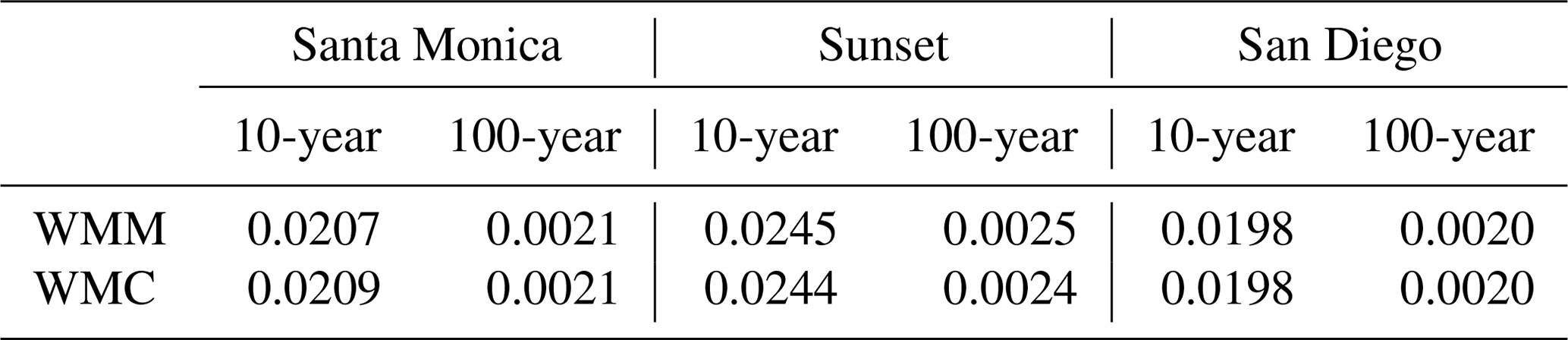
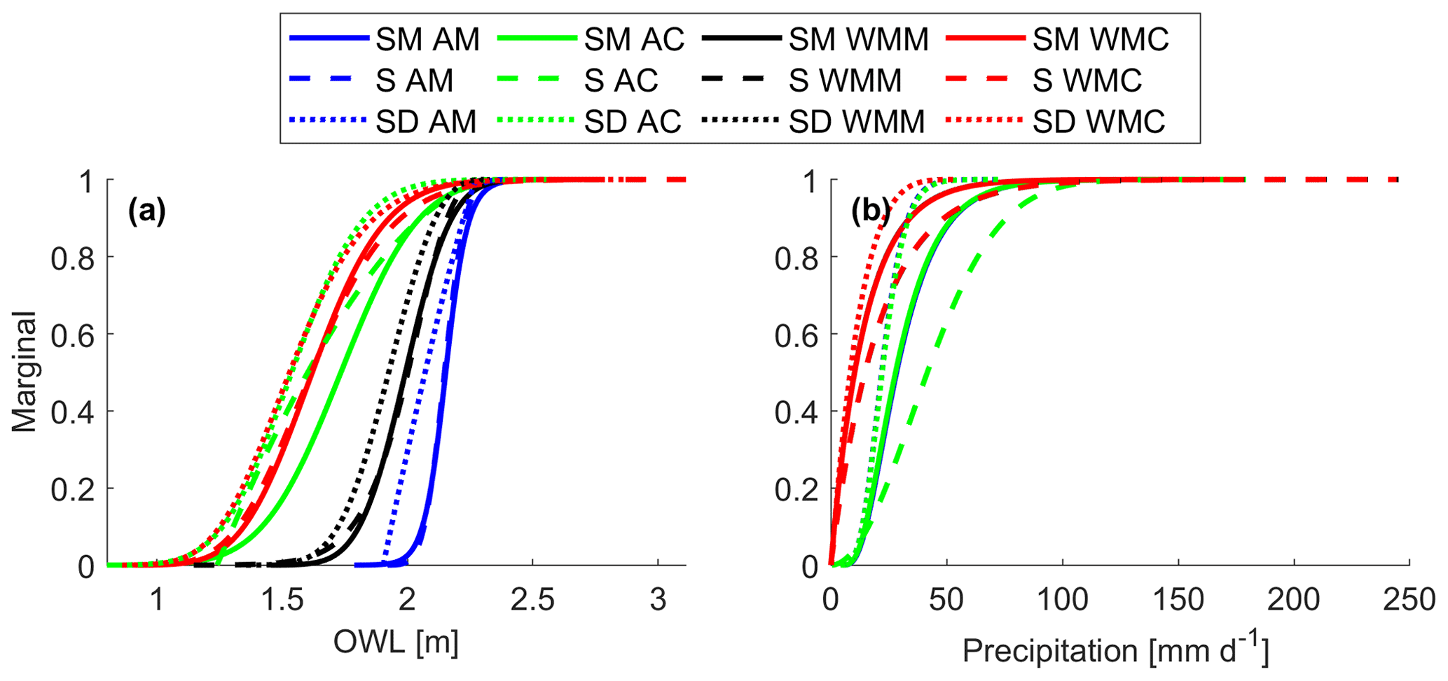
Figure 3 (a) OWL and (b) precipitation marginals for Santa Monica (SM; solid lines), Sunset (S; dashed lines), and San Diego (SD; dotted lines) using annual maximum (AM; blue), annual coinciding (AC; green), wet-season monthly maximum (WMM; black), and wet-season monthly coinciding (WMC; red) samplings.

4.1 Marginals

The selected marginal distributions (Fig. 3, Table 4) were tested and/or suggested fits in previous studies. Rainfall has been widely fit with an exponential distribution (refer to Table 2 in Salvadori and De Michele, 2007) but more recently has been fit using a variety of distributions including Gamma (Husak et al., 2007), Rayleigh (Pakoksung and Takagi, 2017; Esberto, 2018), generalized Pareto, or Birnbaum–Saunders (Ayantobo et al., 2021). In the case of annual precipitation (coinciding or maximum sampling) Santa Monica was well described by a Birnbaum–Saunders, Rayleigh best described Sunset data, and a Gamma was the best fit for San Diego data. Similarly, wet-season precipitation data (maximum or coinciding sampling) were best described by the exponential distribution for Santa Monica and Sunset, while the generalized Pareto best represented San Diego.

Historically, water levels have been described using a number of distributions including normal (Hawkes et al., 2002), generalized Pareto (Mazas and Hamm, 2017), log logistic and Nakagami (Sadegh et al., 2018), and Birnbaum–Saunders (Sadegh et al., 2018; Didier et al., 2019; Jane et al., 2020), along with Gamma, Weibull, and inverse Gaussian (Jane et al., 2020). Observed water levels did not exhibit site-specific patterns and were described by a range of distributions (Table 4).

Table 4 Best-fitting univariate distributions for each location and sampling method (annual maximum, AM; annual coinciding, AC; wet-season monthly maximum, WMM; wet-season monthly coinciding, WMC).

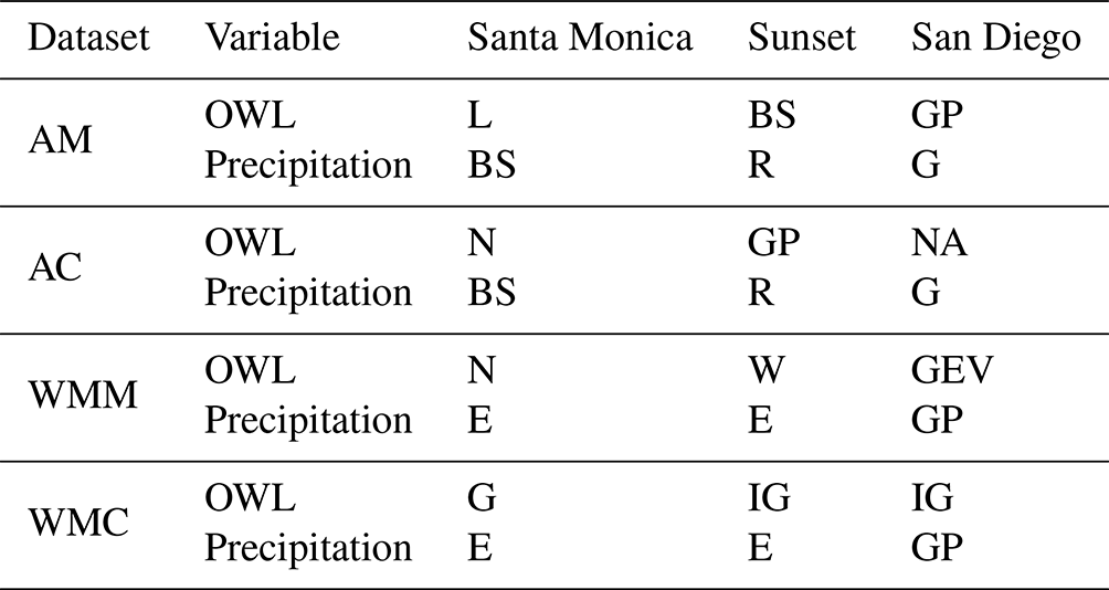
BS – Birnbaum–Saunders, GP – generalized Pareto, E – exponential, R – Rayleigh, N – normal, L – log logistic, G – Gamma, W – Weibull, IG – inverse Gaussian, NA – Nakagami.

4.2 Copulas

San Diego wet-season monthly coinciding conditional CDFs display individual copulas' effects (Fig. 4). The Nelsen, Roch., and BB1 copulas consistently suggest similar OWL (Fig. 4a, e) and precipitation values (Fig. 4b, f), while, in this example, the BB5 suggests higher OWL and precipitation values (solid black line, Fig. 4a, b, e, f). C1's 100-year pair in Table 6 displays an example of the BB5's conservative nature. Copula choice has nearly no effect on the Conditional 2 scenario (Fig. 4c, d). Most probable OWL and precipitation values in Tables 5 and 6 further display the aforementioned behaviors. These conditional patterns generally persist at all locations with an additional note that the Nelsen can suggest lower OWL values, and the BB5 can provide similar results to the Roch. and BB1 copulas.

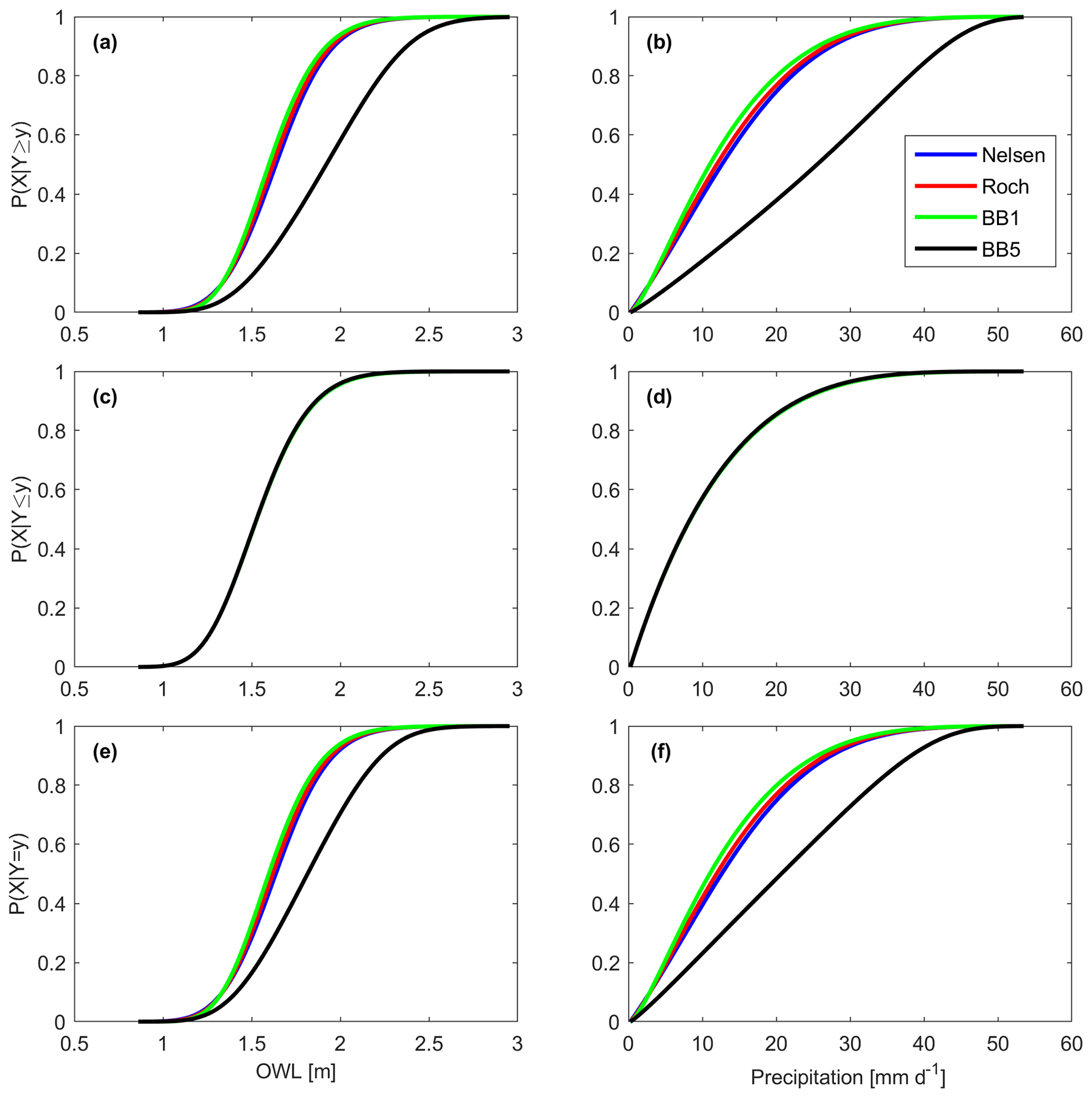
Figure 4 San Diego wet-season monthly coinciding OWL (left column) and precipitation (right column) (a, b) C1, (c, d) C2, and (e, f) C3 CDFs using the Nelsen (blue), Roch–Alegre (Roch), BB1 (green), and BB5 (black) copulas. OWL and precipitation conditionals are conditioned on the occurrence of a 25-year precipitation or OWL event.

Figures 5 and 6 show the 10- and 100-year return periods, respectively, for the four focused copulas using wet-season monthly coinciding sampling at San Diego. Clearly the BB5 presents conservative results, suggesting higher OWL and precipitation pairs in the AND and SK scenarios (Figs. 5a, c and 6a, c), while the BB1, Nelsen, and Roch–Alegre copulas present similar OWL and precipitation values. The OR and Kendall scenarios suggest quite similar isolines between copulas, suggesting similar values, but the BB5 suggests less severe OWL and larger precipitation values according to the densest location along its isoline (Figs. 5b, d, and 6b, d). Tables 5 and 6 further display the bivariate patterns. Again, these bivariate patterns generally persist at all locations with the following additional notes: the Nelsen may suggest lower OWL values in the AND and SK scenarios, the BB5 typically has similar results to the Roch. and BB1 copulas in the AND and SK scenarios, and the BB5 typically agreed with the other copula results outside of San Diego for the OR and K scenarios.

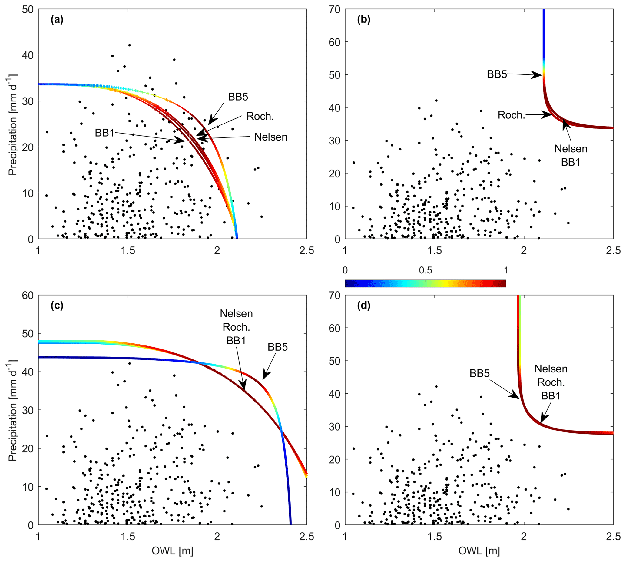
Figure 5 San Diego wet-season monthly coinciding (a) AND, (b) OR, (c) SK, and (d) K hazard scenarios with the Nelsen, Roch–Alegre (Roch), BB1, and BB5 10-year isolines. Copula labels point to the mostly likely value on their respective isolines.

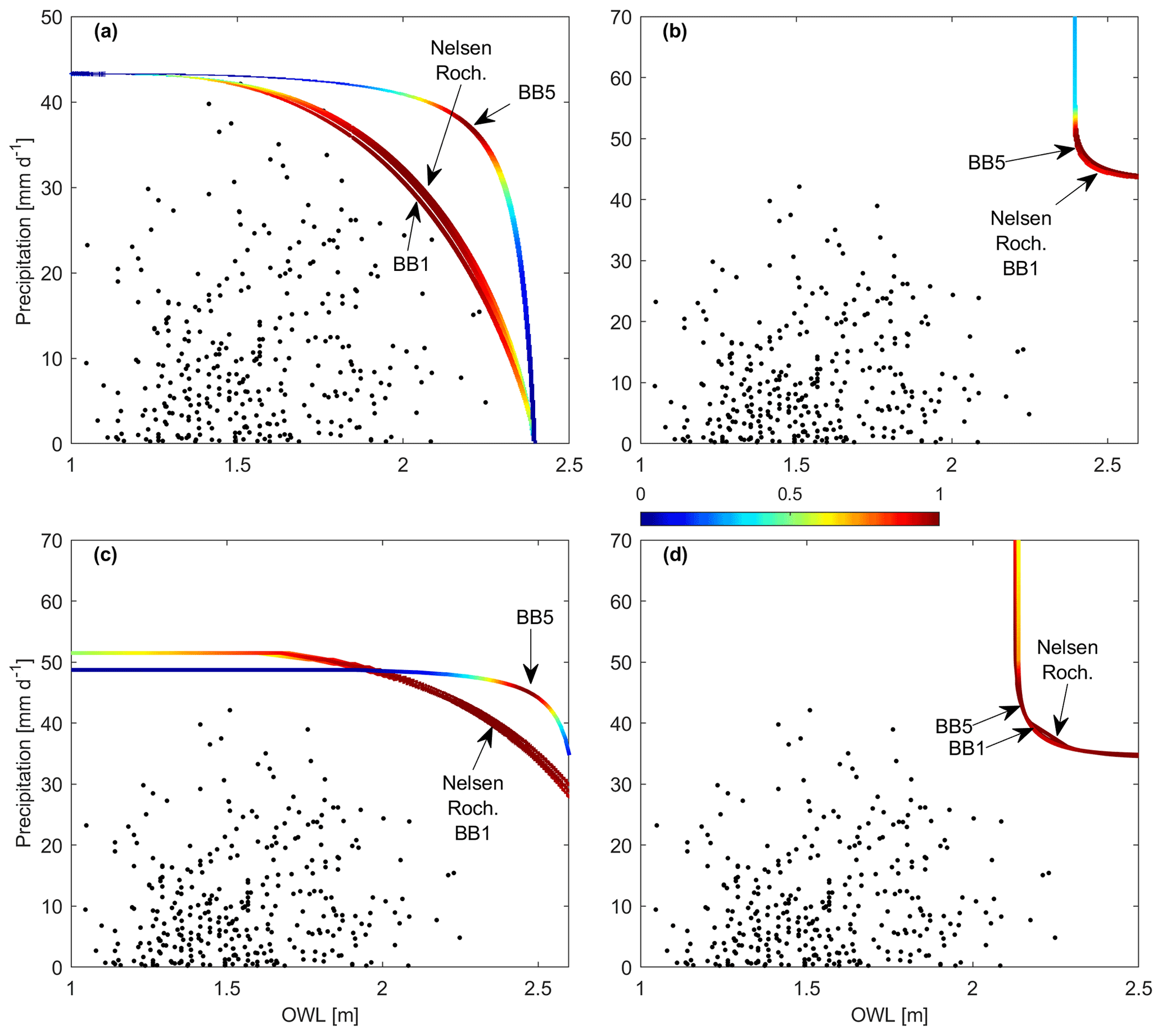
Figure 6 San Diego wet-season monthly coinciding (a) AND, (b) OR, (c) SK, and (d) K hazard scenarios with the Nelsen, Roch–Alegre (Roch), BB1, and BB5 100-year isolines. Copula labels point to the mostly likely value on their respective isolines.

Table 5 San Diego 10-year marginal (M), conditional (C), and bivariate OWL (m) and precipitation (mm d⁻¹) values using wet-season monthly coinciding sampling. Conditionals are conditioned on a 25-year event occurrence.

Table 6 San Diego 100-year marginal (M), conditional (C), and bivariate OWL (m) and precipitation (mm d⁻¹) values using wet-season monthly coinciding sampling. Conditionals are conditioned on a 25-year event occurrence.

4.3 Sampling

San Diego conditional CDFs using the BB1 copula clearly present sampling effects (i.e., maximum versus coinciding and annual versus wet-season months). It should be noted that each sampling method represents a unique probability space and accordingly results in alternative realizations of a given return period. Coinciding samplings exhibit similar OWL CDFs (green and red lines, Fig. 7a, c, e), whereas wet-season samplings exhibit similar precipitation CDFs (red and black lines, Fig. 7b, d, f). OWL values can be larger for maximum samplings at lower non-exceedance probabilities (i.e lower return periods) (Fig. 7a, c, e, blue and black lines; Table 7). However, the extended tail from WMC sampling produces larger OWL at higher return periods (red line Fig. 7a, c, e; Table 8). Annual coinciding sampling displays significantly lower OWL values at low (Table 7) and high (Table 8) return periods. Only minimal differences between annual and wet-season precipitation exist at the 10- and 100-year return periods (maximum difference of 1.06 and 4.56 mm d⁻¹, respectively; Tables 7 and 8). Annual (wet season) precipitation CDFs appear similar as OWL measurements are chosen subsequent to precipitation observations (Fig. 7b, d, f).

Figure 7 San Diego OWL (left column) and precipitation (right column) (a, b) C1, (c, d) C2, and (e, f) C3 CDFs for annual maximum (AM; blue), annual coinciding (AC; green), wet-season monthly maximum (WMM; black), and wet-season monthly coinciding (WMC; red) samplings using the BB1 copula. OWL and precipitation conditionals are conditioned on the occurrence of a 25-year precipitation or OWL event.

Figures 8 and 9 present the 10- and 100-year return periods using the BB1 copula for all samplings (AM, AC, WMM, and WMC). For the AND and K scenarios, AM sampling results in the largest OWL compared to the other sampling methods (Figs. 8a, d and 9a, d, Tables 7 and 8). Additionally for the AND and K scenarios (Fig. 8a, d and 9a, d), maximum samplings (AM and WMM) provide more conservative OWLs compared to WMC OWL values (Tables 7 and 8). When comparing maximum samplings (AM and WMM) to WMC sampling in the OR and SK scenarios, maximum samplings generally provide larger OWL values at lower return periods (Fig. 8b, c, Table 7) but smaller or similar OWL at larger return periods (Fig. 9b, c; Table 8). AC sampling generally results in the smallest OWL levels at all hazard scenarios. These behaviors persist across all locations. Given that wet-season monthly coinciding sampling results in larger OWL values for the marginal, conditional, OR, and Kendall scenarios, this suggests that maximum-type sampling may not accurately reflect OWL at extreme return periods.

Figure 8 San Diego (a) AND, (b) OR, (c) SK, and (d) K hazard scenarios for annual maximum (AM; cross), annual coinciding (AC; plus), wet-season monthly maximum (WMM; dot), and wet-season monthly coinciding (WMC; triangle) data and 10-year isolines using the BB1 copula. Sampling labels point to the mostly likely value on their respective isolines.

Figure 9 San Diego (a) AND, (b) OR, (c) SK, and (d) K hazard scenarios for annual maximum (AM; cross), annual coinciding (AC; plus), wet-season monthly maximum (WMM; dot), and wet-season monthly coinciding (WMC; triangle) data and 100-year isolines using the BB1 copula. Sampling labels point to the mostly likely value on their respective isolines.

Tables 7 and 8 show the most probable 10- and 100-year marginal and multivariate event values. AM OWL exceeds AC OWL across all probability types and sites, which is expected given the (nonphysical) paring of the two largest individual OWL and precipitation events without regard to co-occurrence. For example, in the 10-year return period annual maximum OWLs are at least 30 cm higher than AC (Table 7). In the 100-year return period annual maximum OWLs exceed annual coinciding OWLs by at least 17 cm (Table 8). Precipitation is generally consistent across sampling types with only minor variations observed. AM and WMM sampling generally produced similar OWL results at both the 10- and 100-year return periods with a maximum difference of 6 cm across all conditionals and copulas.

Table 7 San Diego 10-year marginal (M), conditional (C), and bivariate OWL (m) and precipitation (mm d⁻¹) values using the BB1 with annual maximum (AM), annual coinciding (AC), wet-season monthly maximum (WMM), and wet-season monthly coinciding (WMC) samplings. Conditionals are conditioned on a 25-year event occurrence.

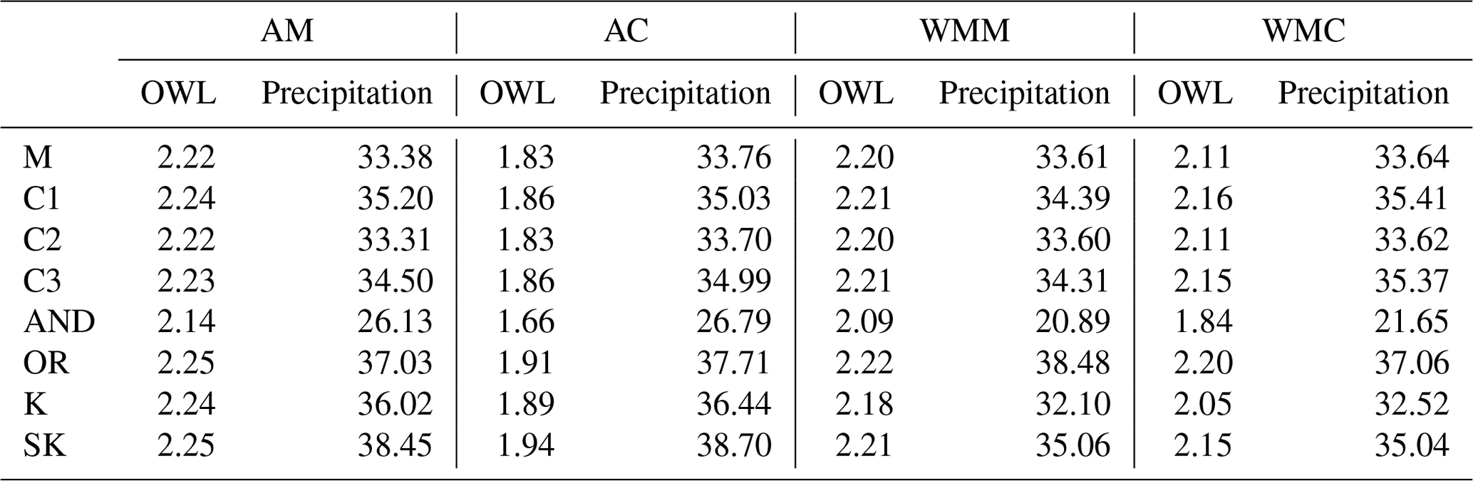
Table 8 San Diego 100-year marginal (M), conditional (C), and bivariate OWL (m) and precipitation (mm d⁻¹) values using the BB1 with annual maximum (AM), annual coinciding (AC), wet-season monthly maximum (WMM), and wet-season monthly coinciding (WMC) samplings. Conditionals are conditioned on a 25-year event occurrence.

4.4 Structural failure

A structural scenario is presented to consider flood severity along the Pacific Coast Highway (PCH) in Sunset Beach. PCH road elevation ranges from 1.7–2.4 m NAVD88 (Fig. 10), below typical spring tide (∼ 2.13 m) and more extreme (∼ 2.3 m) water levels (NOAA, 2021b), requiring tide valves along the PCH for flood prevention. Tide valve closures prevent back-flooding from high bay water levels coming up through subsurface storm drains that (normally) discharge to the bay. Additionally, closed tide valves enable precipitation pooling since water cannot be drained to the bay. Severe pooling may result in a critical highway closure, which can further damage property and inhibit emergency service operations.

Areal precipitation flooding extent and depth can be estimated for water levels exceeding tide valve closure elevation. A water level equal to or greater than 1.68 m NAVD88 forces valve closures and frames the structural failure as a Conditional 1-type event. The local watershed is convex and drains an area of 94 897 m². Water pools in the low-elevation areas along the PCH (Fig. 10). When pluvial water levels exceed the sea wall elevation, water overflows the sea wall and exits to the harbor. The maximum pool storage is 11 342 m³. The percent of flooding is then calculated with Eq. (20) as the structural function.

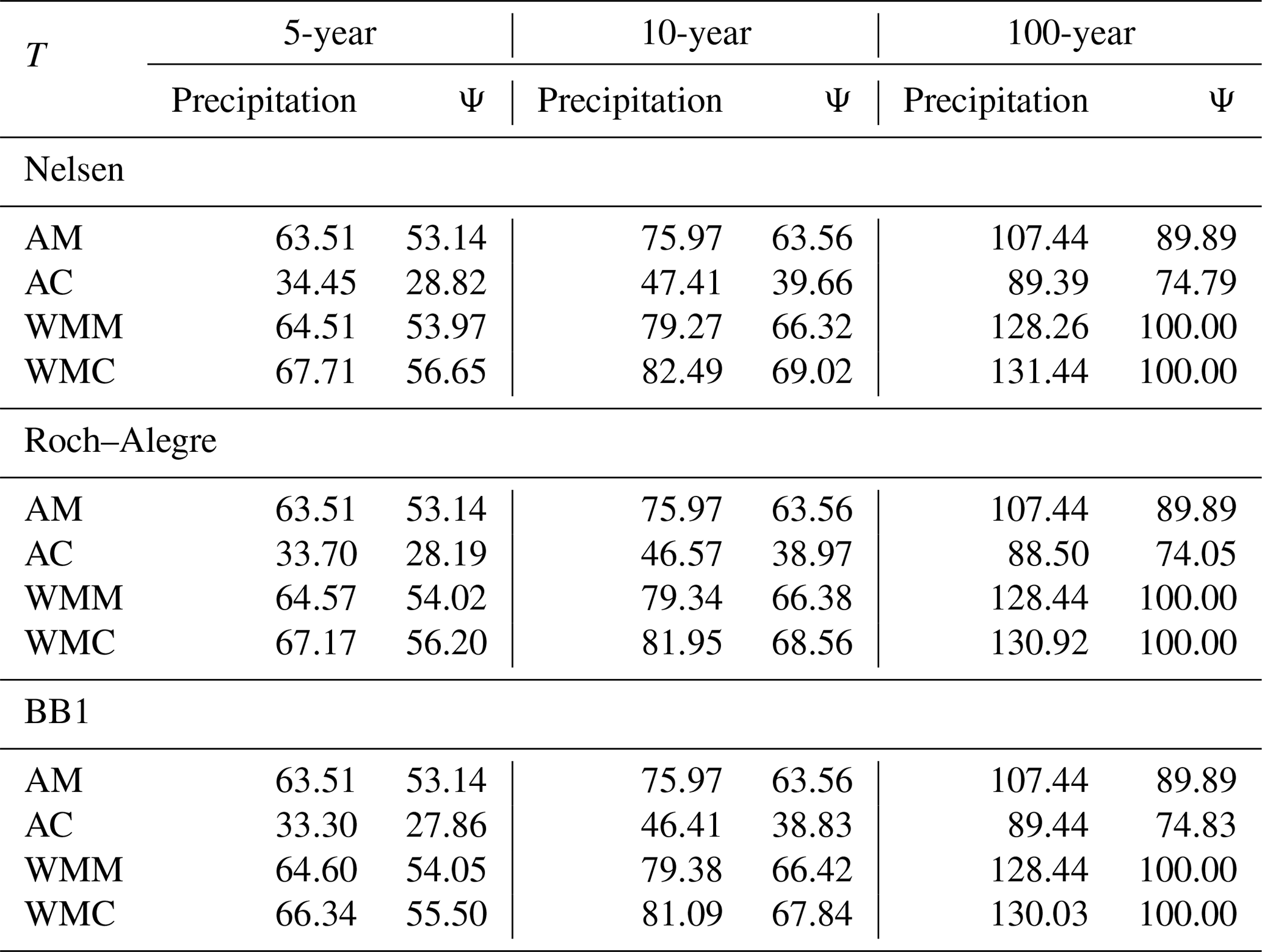
Structural scenario precipitation and percent flooding (Ψ) values utilizing the Nelsen, Roch–Alegre, and BB1 copulas are shown in Table 9. Rows and columns separate the utilized sampling methods and return periods of interest, respectively. Figure 11 shows Ψ as a function of precipitation for the Nelsen, Roch–Alegre, and BB1 copulas along with the 5- (square), 10- (circle), and 100-year (diamond) return periods. All copulas display similar values across sampling methods (Fig. 11, Table 9). For example, the 10-year precipitation with wet-season monthly coinciding sampling is 82.49, 81.95, and 81.09 for the Nelsen, Roch–Alegre, and BB1 copulas, respectively. Again, AC sampling severely underestimates precipitation and flooding.

$$\begin{array}{}\text{(20)}& \mathit{\%}\mathrm{flooding}={\displaystyle \frac{\mathrm{precipitation}\times \mathrm{area}}{\mathrm{volume}}}\times \mathrm{100}\end{array}$$

Figure 10 Elevations within the Pacific Coast Highway boundary ranging from low (purple) to high (blue). Background imagery from NOAA (2021a).

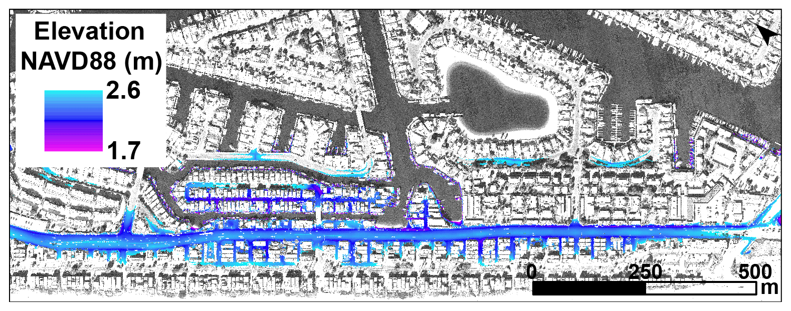
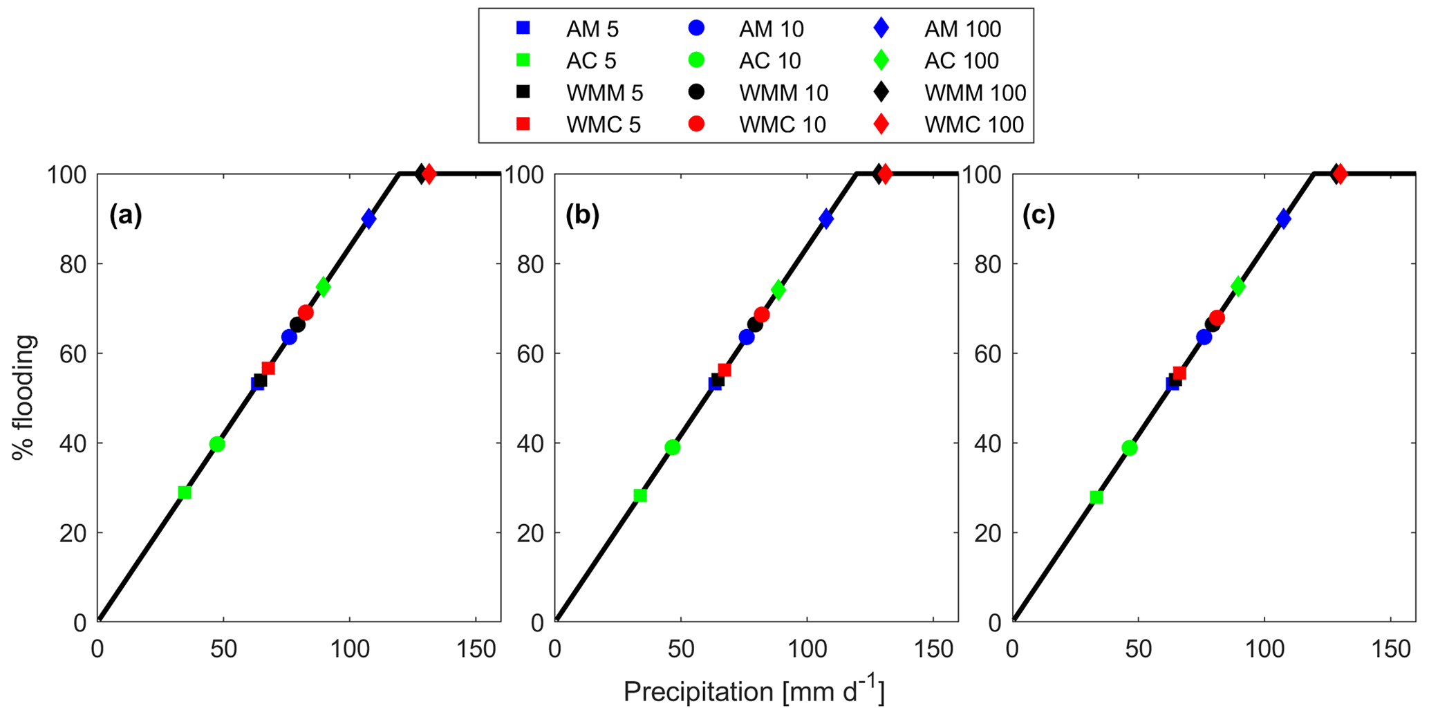
Figure 11 Structural scenario 5- (square), 10- (circle), and 100-year (diamond) return periods for annual maximum (AM; blue), annual coinciding (AC; green), wet-season monthly maximum (WMM; black), and wet-season monthly (WMC; red) data using the (a) Nelsen, (b) Roch–Alegre, and (c) BB1 copulas.

Table 9 Precipitation and percent flooding (Ψ) associated with the 5-, 10-, and 100-year return periods (T) using the Nelsen, Roch–Alegre, and BB1 copulas to determine C1 values with annual maximum (AM), annual coinciding (AC), wet-season monthly maximum (WMM), and wet-season monthly coinciding (WMC) samplings. Precipitation values are in millimeters per day, and Ψ is a percentage. Values are based off an OWL of ≥ 1.68 m, which forces tide valve closure.

5 Discussion

Previous multivariate studies typically use a small, popular group of copulas (e.g., Clayton, Frank, Gumbel, Student t, and Gaussian). Gaussian and Student t copulas were excluded from this study due to their lack of a computationally simple derivative or integral, while the Clayton, Frank, and Gumbel failed to pass the Cramér–von Mises test. Nelsen, BB1, BB5, and Roch–Alegre copulas generally present similar values, with the BB5 occasionally presenting more conservative pairs (Fig. 6). Well-fit copulas concentrate probabilities around more centralized OWL and precipitation values for multivariate events. This is most pronounced at higher (i.e., 100-year) return periods (Fig. 6). The fact that the resulting copulas exhibit agreement between values (for a given sampling) suggests that choosing a reasonable copula may be sufficient to provide a robust characterization of considered multivariate flooding events.

The choice in sampling imparts a significant influence on event risk interpretation. When maximum versus coinciding sampling is considered, maximum samplings (AM and WMM) tend to provide the largest OWL at low return periods (Figs. 7a, c, e and 8, Table 7). At larger return periods, wet-season monthly coinciding then provides significantly larger OWLs (Figs. 7a, c, e and 9, Table 8). This is observed in the conditionals and bivariates (minus the AND and K hazard scenarios, whose maximum samplings display the largest OWLs) at all sites. From a logical perspective, coinciding sampling provides a more realistic view of multivariate events (by definition these are pairs that have co-occurred to produce a multivariate flooding event). At long return periods annual coinciding sampling may require a long data record, which is often unavailable. Notably, in this study annual coinciding produced OWL samplings that were substantially lower than any of the other samplings. For example when comparing 100-year OWLs with annual and wet-season monthly coinciding samplings, the marginal was 32 cm lower, and the AND scenario was 17 cm lower (Table 8). Given that sea-wall-protected urban coastal areas are highly sensitive to even minor elevation differences (e.g., Gallien et al., 2011), this suggests that with limited data records annual coinciding sampling should be avoided.

An important note is that each probability type appropriately describes a unique event, characterized by OWL and precipitation. Serinaldi (2015) suggests that inter-comparing univariate, multivariate, and conditional probabilities and return periods is misleading as each probability type describes its associated event. Events where only extreme OWL or precipitation is of concern should simply utilize marginal statistics and follow current FEMA guidelines. Multivariate event analysis may utilize a variety of scenarios. Conditional-type distributions become useful when future information on one variable is known (e.g., predicted OWL levels). AND scenarios may be applied when both variables exceeding given limits are of concern. The survival Kendall scenario is an alternative to the AND scenario using a more conservative approach to develop events of concern (Salvadori et al., 2013). An OR scenario should be applied when either multivariate variable exceeding a limit is of concern, whereas the Kendall scenario provides minimum OR events of concern (Salvadori et al., 2011). The benefit of the Kendall and survival Kendall is that all the events along their isolines describe a similar probability space versus the AND, and OR isolines describe events with similar probabilities of non-exceedance. It is critical for practitioners and future studies to define concerning flood events within a region since the associated probability will result in varying event risk estimates, as seen within this work. The selected probability type will have significant influence on flood risk studies and modeling efforts. A majority of previous studies focus on specific probability types and do not consider multiple flooding pathways. Only a single study explores all the probabilities associated with different extreme events (Serinaldi, 2016).

From a regulatory perspective, FEMA recommends individual (univariate) analysis to develop return periods for multivariate coastal flooding applications (FEMA, 2011, 2016c, 2020) and blending the two hazard mapping results. Fundamentally, this type of approach assumes (event) independence and may underestimate multivariate flood hazards (e.g., Moftakhari et al., 2019; Muñoz et al., 2020). FEMA provides guidelines for coastal-riverine- (FEMA, 2020), tide-, surge-, tide-surge- (FEMA, 2016a), surge-riverine- (FEMA, 2016c), and tropical-storm (or hurricane)-type flooding events (FEMA, 2016b). Currently, FEMA does not provide specific guidance for considering high marine water levels and precipitation. However, this work suggests that at high return periods the sampling method is critical to characterizing both univariate and joint probabilities.

Structural scenarios provide a quantitative context to frame flood vulnerability. In the structural failure context, annual coinciding sampling significantly underestimates flooding at all return periods, and annual maximum sampling underestimates severe (i.e., 100-year) events, echoing previous annual maximum and coinciding sampling issues. Similar values between most copulas support the suggestion that choosing a reasonable copula will provide robust results in these types of applications. Precipitation events in the structural scenario (Table 9) range between 33.30 mm d⁻¹ and 131.44 mm d⁻¹, resulting in between 27.86 % and complete (100 %) backshore flooding. This significant flooding at all return periods suggests severe flood vulnerability, which is validated by frequent closures of the PCH. This structural function provides a quick and simple alternative to poorly performing bathtub flood models (e.g., Bernatchez et al., 2011; Gallien et al., 2011, 2014; Gallien, 2016) to quantitatively explore flood severity while accounting for infrastructure and joint probabilities.

The maximum OWL and precipitation observations within the record are 2.33 m and 118.93 mm d⁻¹ for Sunset, 2.27 m and 42.11 mm d⁻¹ for San Diego, and 2.45 m and 76.83 mm d⁻¹ for Santa Monica. Most likely precipitation and OWL pairs in high return periods often exceed the current data record's maximums (e.g., Table 8). This study is limited to the available data records, and sea level rise clearly imparts a non-stationary trend. Current water level values restricted to today's distribution tails will become more frequent in the next century (Taherkhani et al., 2020). For example, Wahl et al. (2015) suggest that a previously 100-year event in New York is now a 42-year event based on the increasing correlation between extreme precipitation and storm surge events. Similarly, our results suggest increasing precipitation and, particularly, OWL levels.

6 Conclusions

Univariate and multivariate event risks from OWL and/or precipitation were explored at three sites in a tidally dominated, semi-arid region. Seventeen copulas were considered. Previous studies typically relied upon a small number of copulas (e.g., Clayton, Frank, Gumbel, Student t, and Gaussian) for multivariate flood assessments. In this case, the Nelsen, BB1, BB5, and Roch–Alegre copulas passed the Cramér–von Mises test and produced similar, quality fits across all sampling methods. However, in some cases, the BB5 produced conservative results. Copulas exhibit similar most probable pairs (e.g., Figs. 5, 6), suggesting that a number of potential copulas may provide a robust multivariate analysis. The impact of sampling and distribution choice on uni- and multivariate return period values are presented; however uncertainties deserve further characterization. This work focused solely on exploring conditional and joint probabilities of OWL and precipitation in a tidally and wave-dominated semi-arid region and would not be applicable to regions experiencing multiple flooding seasons (e.g., Couasnon et al., 2022). Although wave impacts were not included in this assessment, they are fundamental to coastal flooding, particularly in regions subjected to long-period swell. Joint probability methods explicitly including wave contributions to multivariate event risk characterizations are needed for future work.

The annual maximum method is widely recognized for hazard assessments (FEMA, 2011, 2016c) and is common practice in flood risk analysis (e.g., Baratti et al., 2012; Bezak et al., 2014; Wahl et al., 2015). Concerningly, this work suggests that annual maximum sampling does not characterize severe flooding potential for extreme events. Water levels are substantially underestimated as annual sampling neglects a large portion of observations (Table 8). Generally, maximum samplings produced larger values at minor return periods but significantly underestimated water levels at longer return periods than wet-season monthly coinciding sampling. Similarly, annual-coinciding-type sampling (Tables 7, 8) grossly underestimates OWLs. Wet-season sampling quadruples data pairs (Table 2), providing additional historical joint event information. Further investigation into monthly coinciding and, where appropriate, water year coinciding is needed to develop optimal sampling strategies for given regional conditions.

Appendix A: Additional BICs

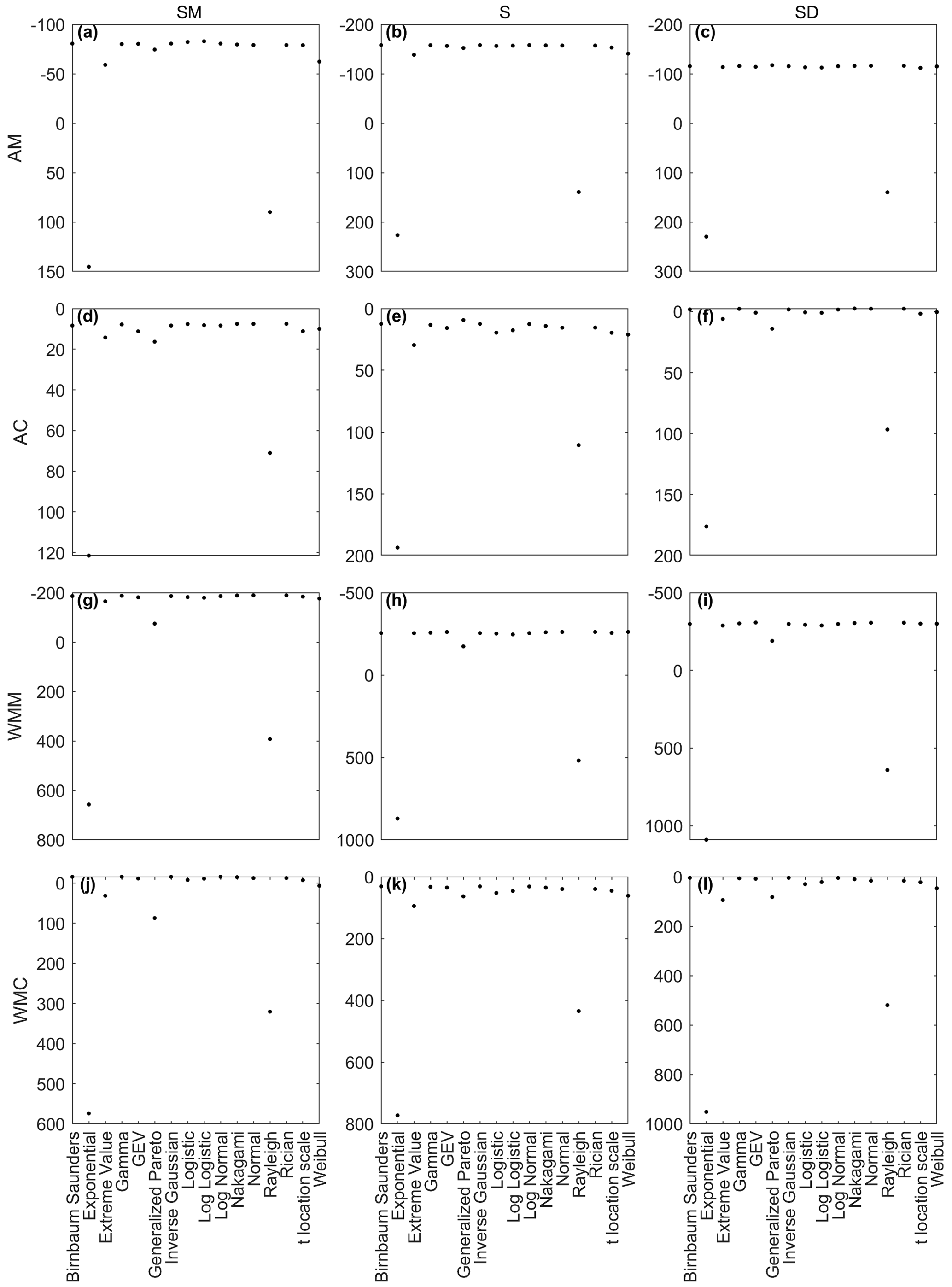
Figure A1 Marginal OWL BIC values per fitted copula for Santa Monica (left column), Sunset (middle column), and San Diego (right column) using annual maximum (a, b, c), annual coinciding (d, e, f), wet-season monthly maximum (g, h, i), and wet-season monthly coinciding (j, k, l). The y axis is oriented to display best BIC (top) to worse BIC (bottom).

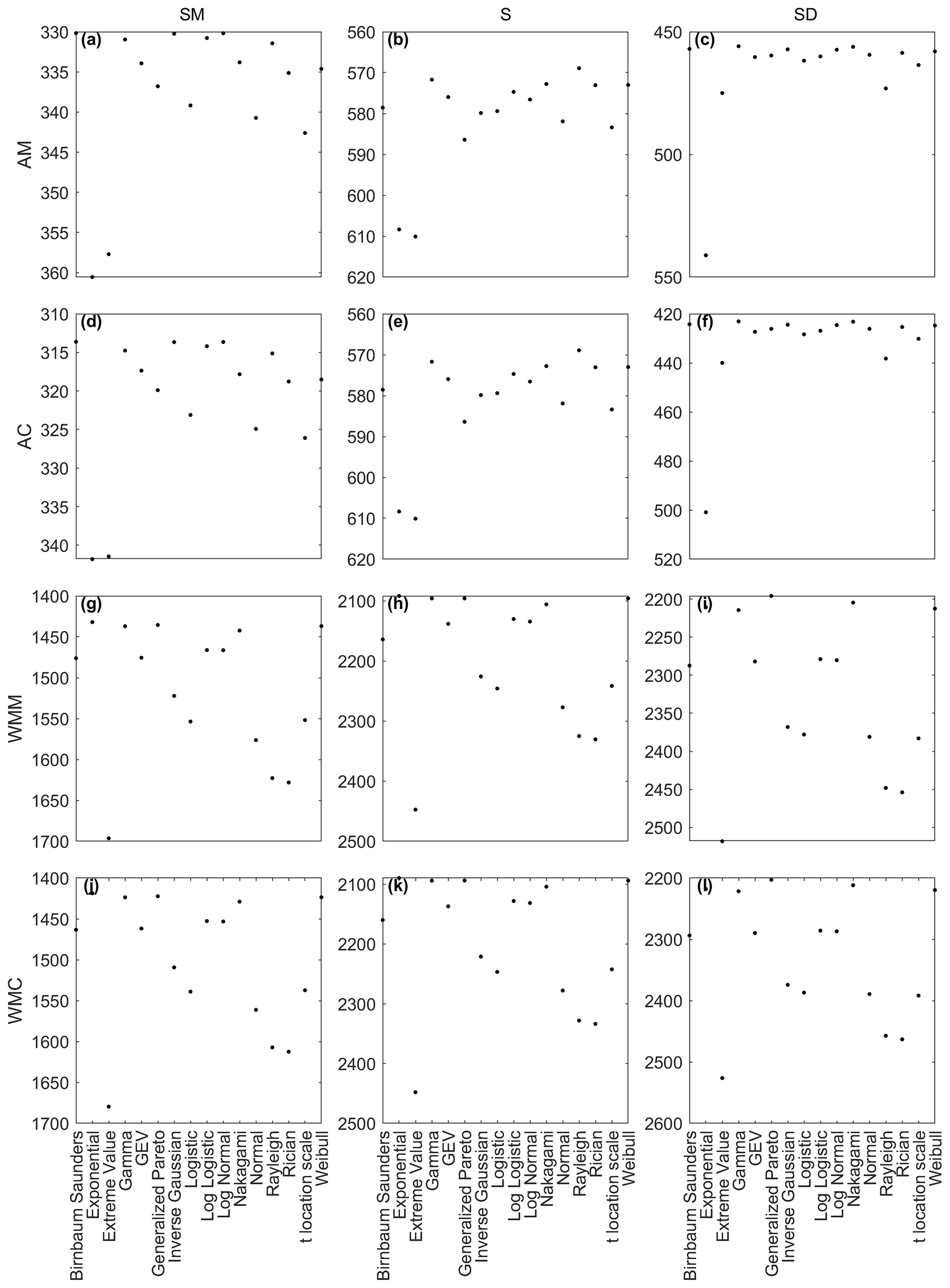
Figure A2 Marginal precipitation BIC values per fitted copula for Santa Monica (left column), Sunset (middle column), and San Diego (right column) using annual maximum (a, b, c), annual coinciding (d, e, f), wet-season monthly maximum (g, h, i), and wet-season monthly coinciding (j, k, l). The y axis is oriented to display best BIC (top) to worse BIC (bottom).