Machine-learning blends of geomorphic descriptors: value and limitations for flood hazard assessment across large floodplains

Recent literature shows several examples of simplified approaches that perform flood hazard (FH) assessment and mapping across large geographical areas on the basis of fast-computing geomorphic descriptors. These approaches may consider a single index (univariate) or use a set of indices simultaneously (multivariate). What is the potential and accuracy of multivariate approaches relative to univariate ones? Can we effectively use these methods for extrapolation purposes, i.e., FH assessment outside the region used for setting up the model? Our study addresses these open problems by considering two separate issues: (1) mapping flood-prone areas and (2) predicting the expected water depth for a given inundation scenario. We blend seven geomorphic descriptors through decision tree models trained on target FH maps, referring to a large study area (∼ 10⁵ km²). We discuss the potential of multivariate approaches relative to the performance of a selected univariate model and on the basis of multiple extrapolation experiments, where models are tested outside their training region. Our results show that multivariate approaches may (a) significantly enhance flood-prone area delineation (accuracy: 92 %) relative to univariate ones (accuracy: 84 %), (b) provide accurate predictions of expected inundation depths (determination coefficient ∼ 0.7), and (c) produce encouraging results in extrapolation.

1 Introduction

Every year flood events worldwide cause vast economic losses as well as heavy social and environmental impacts, which have been steadily increasing over the last 5 decades (Jongman et al., 2014; Guha-Sapir et al., 2016), mainly because of the complex interaction between the intensification of extreme hydrological events due to climate change (e.g., Brunetti et al., 2002; Uboldi and Lussana, 2018) and anthropogenic pressure (i.e., land-use and land-cover modifications; see Di Baldassarre et al., 2013; Domeneghetti et al., 2015; Requena et al., 2017). Thus, nowadays, successful flood hazard mapping for flood hazard management is a major task for the whole scientific community (Alfieri et al., 2014; Dottori et al., 2016). Traditional methods to assess fluvial flood hazard rely on hydrological and hydraulic numerical models, whose improvement allows the simulation of any scenario for different geometrical or hydrological conditions, obtaining very accurate results (Horritt and Bates, 2002; Costabile et al., 2012; Bellos and Tsakiris, 2016). However, a high amount of hydrologic and hydraulic input information is required to adequately describe the geometry and hydraulic behaviour of the system; thus considerable effort and computation capacity are needed. Consequently, numerical models are unsuitable for large-scale applications and in data-scarce regions. To overcome this issue, other mapping techniques have been proposed that take advantage of the wealth of topographic information contained in digital elevation models (DEMs): flood-related geomorphic descriptors (or features or indices) can be derived from DEMs and used to obtain a measure of flood hazard. The first DEM-based approaches proposed in the literature (see, e.g., Williams et al., 2000; Noman et al., 2001; Dodov and Foufoula-Georgiou, 2006; Nardi et al., 2006; Manfreda et al., 2011, 2014, 2015; Samela et al., 2017; and De Risi et al., 2018) consider a single geomorphic index (these approaches are referred to as univariate hereafter), which is used as a binary classifier to distinguish between flood-prone and flood-free areas through the definition of a threshold value. The optimal threshold value is identified by means of an iterative calibration procedure, which optimizes the agreement of the binary map with a reference pre-existing flood hazard map obtained, for example, from hydrological–hydraulic numerical simulations. Several authors (see, e.g., Manfreda et al., 2015, and Samela et al., 2017) highlight that the performance of the considered geomorphic index can change according to the geographical context of the application. In particular, the descriptor named geomorphic flood index (GFI; Samela et al., 2017) has been shown to have good effectiveness in mountainous as well as in predominantly flat areas and thus has been used extensively by many authors for developing web services, platforms, and geographic information system (GIS) tools for flood hazard mapping applications (Samela et al., 2018; Tavares da Costa et al., 2019). A second class of DEM-based approaches to be investigated can be named as multivariate as they rely on the combination of different geomorphic descriptors (GDs). The relation between the combination of GDs and flood hazard can be searched through numerous statistical methods. Commonly, machine-learning (ML; Breiman, 1984) models are used, often ensembled with multi-criteria decision-making techniques (Triantaphyllou et al., 2000; Ho et al., 2010). Some authors (Degiorgis et al., 2012; Gnecco et al., 2017) have tested a blend of GDs, while some others mixed these indices with information on land use, soil geology, and climate and compared different combination strategies (e.g., Wang et al., 2015; Lee et al., 2017; Khosravi et al., 2018; Arabameri et al., 2019; Janizadeh et al., 2019; Costache et al., 2020). These studies suggest that data-driven flood hazard mapping has a remarkable potential. However, in most of the studies, the reference flood hazard information used to set up the models consists of a dataset of isolated historical events observed in the study area (Lee et al., 2017; Khosravi et al., 2018; Janizadeh et al., 2019; Arabameri et al., 2019; Costache et al., 2020), leading to case-specific prediction skills.

Important advantages of DEM-based flood hazard mapping methods are their flexibility and, in principle, their general applicability to any flood-prone area where a reliable DEM is available as well as their low computational costs relative to numerical models. However, two main drawbacks must be highlighted: first, DEM-based methods do not consider the water dynamics, and second, they need a pre-existing reliable reference flood hazard map, which may or may not be available for the area of interest. Overall, DEM-based models are very useful as preliminary flood hazard mapping tools in data-scarce contexts and for application in large areas but cannot yet effectively substitute the traditional models, especially when detailed results are required. Nevertheless, if a strong and reliable relation to derive flood hazard from GDs is obtained, the model could be easily applied in extrapolation to any region where the same relation is supposed to be valid (Tavares da Costa et al., 2020).

In this study, multivariate DEM-based flood hazard mapping is investigated. We consider a large study area (10⁵ km²) in northern Italy, which is characterized by markedly different morphological, hydrological, and climatic conditions. We use the ∼90 m resolution, hydrologically corrected MERIT DEM (Yamazaki et al., 2017) for deriving a set of GDs. We then use decision trees, a common machine-learning technique (Hastie et al., 2009), for assessing flood hazard associated with a given probability of occurrence (i.e., return period) in terms of (a) delineation of flood-prone and flood-free areas and (b) prediction of expected inundation water depth (as a measure for flood intensity). The simultaneous combination of the five following meaningful elements makes our study different from all previous works in the literature. First, only strictly easy-to-retrieve, DEM-based GDs are used to assess flood hazard, in contrast with several studies in which also other information is considered. Second, both generation of binary flood susceptibility maps and prediction of expected maximum inundation water depth are analysed, setting up parallel models. Third, decision trees are trained using pre-existing flood hazard maps as target information, in contrast with the discontinuous datasets of historical events mostly used to train machine-learning models for flood hazard estimation (Lee et al., 2017; Khosravi et al., 2018; Janizadeh et al., 2019; Arabameri et al., 2019; Costache et al., 2020). Fourth, a univariate geomorphological approach for identification of flood-prone and flood-free areas (i.e., GFI) is compared with the proposed multivariate approach: this allows us to analyse the actual enhancement resulting from the use of multiple GDs. Fifth, predictive skill of the multivariate DEM-based flood hazard approach is assessed in extrapolation by applying models trained on specific geographical areas to different regions with dissimilar morphological and/or hydrological features. This last aspect is highly important for possible future applications in data-scarce environments in extrapolation mode.

By assuming the above-mentioned characteristics, this study aims to advance previous knowledge on the potential of ML techniques for combining GDs to derive accurate flood susceptibility maps across large geographical regions. More precisely, we want to investigate three main research questions: (1) whether we can we profit from a blend of various GDs for flood hazard assessment and mapping relative to a univariate approach, (2) whether we can we use simple ML techniques for effectively blending multiple GDs, (3) whether these techniques are capable of providing a reliable assessment of flood hazard over large geographical areas when used in geographical extrapolation. What are the desired characteristics of the training region or watershed to make the trained model as general as possible?

The paper is organized as follows: Sect. 2 describes the methods (GDs and decision trees), Sect. 3 illustrates the study area and data, Sect. 4 details the analyses we performed, Sect. 5 shows the results, and Sect. 6 discusses them.

2 Methods

The analyses conducted in the study are based on two main elements: geomorphic descriptors (GDs) and decision trees (DTs); simplicity and replicability of these elements represent a fundamental aspect and an important advantage of this contribution. Aiming to estimate flood hazard output variables (i.e., flood susceptibility and maximum expected water depth), DT models combine several selected DEM-derived input features (GDs) based on the availability of target information (i.e., flood hazard reference maps). Consistent with the aims of our study, we set up two different types of DTs: classifier DTs to solve the classification problem relative to flood-extent delineation and regressor DTs to solve the regression problem of water depth estimation. Classifier and regressor models use the same input GDs but require different target flood hazard maps. The software we use for the training is Scikit-learn (Pedregosa et al., 2011), an open-source library for Python 3.6 or later (Van Rossum et al., 1995).

2.1 Geomorphic descriptors

Topographical rasterized information contained in DEMs can be used to extract GDs adopting several algorithms available in the literature (e.g., Tarboton et al., 1991). These descriptors vary spatially, assuming different values for different pixels within the domain while being constant in time. They can be divided into two broad categories: (1) single features if they represent simple terrain characteristics and (2) composite indices if they are derived based on a combination of other features. As input variables for the above-mentioned models, in our study we use the ground elevation in metres above sea level itself (as retrieved from the DEM) together with six GDs, the first three of which are single indices, while the remaining three are composite:

1. local slope (sd8), estimated for each cell as the maximum slope among the eight possible flow directions and computed as the ratio between the vertical and the horizontal differences;

2. horizontal distance from the nearest stream (D), defined as the length of the path that hydrologically connects each cell to the nearest cell of the river network;

3. height above the nearest drainage (HAND), defined as the vertical difference between a given cell and the hydrologically nearest cell belonging to the river network (Rennò et al., 2008);

4. modified topographic index (TI_m), derived from the modification proposed by Manfreda et al. (2008) to the index originally introduced by Kirkby (1975) and defined as

   $$\begin{array}{}\text{(1)}& {\mathrm{TI}}_{\mathrm{m}}=\ln \left({\displaystyle \frac{a_{\mathrm{d}}^n}{\tan \left(\mathit{\beta }\right)}}\right),\end{array}$$

   where a_d is the drained area per unit contour length, tan (β) is the local gradient, and n is an exponent;

5. geomorphic flood index (GFI), defined as the ratio between the term h_r and HAND (the numerator represents the water depth, computed in the hydrologically nearest stream section with a hydraulic scale relation $h_r\mathit{\approxeq }b{A}_r^n$, where A_r is the contributing area in the considered stream section; coefficient b and exponent n can be appropriately estimated with calibration or taken from the literature; Nardi et al., 2006),

   $$\begin{array}{}\text{(2)}& \mathrm{GFI}=\ln \left({\displaystyle \frac{h_r}{\mathrm{HAND}}}\right);\end{array}$$

6. alternative version of the GFI, hereinafter referred to as local geomorphic flood index (LGFI), defined as

   $$\begin{array}{}\text{(3)}& \mathrm{LGFI}=\ln \left({\displaystyle \frac{h_l}{\mathrm{HAND}}}\right),\end{array}$$

   where the water depth h_l is computed with reference to the contributing area of the considered pixel.

The choice of the above-mentioned GDs is due to different reasons. First, previous studies (e.g., Manfreda et al., 2015; Samela et al., 2017) clearly showed that D and HAND are the most descriptive single-feature indices for flood hazard mapping, sufficiently accurate in mountainous regions but still inadequate over predominantly flat areas, whereas, among composite feature indices, GFI and LGFI show good performance in both the geographical contexts. Also, in several studies (e.g., Wang et al., 2015; Lee et al., 2017; Khosravi et al., 2018; Janizadeh et al., 2019; Costache et al., 2020), elevation retrieved from DEMs is shown to have a strong influence on flood occurrence. Slope appears to be the most important index in Khosravi et al. (2018) and Costache et al. (2020) and among the most influential ones in Arabameri et al. (2019). The adoption of TI_m is based on Manfreda et al. (2008), who highlighted a strong correlation between the index and the occurrence of inundation events.

Indeed, we believe that the selected set of GDs provides DT models with a rather exhaustive description of the study area morphology. In fact, slope and TI_m may influence the infiltration time and consequently the runoff; elevation is not only strongly linked to the runoff but also to climatic conditions; D and HAND consider the horizontal and vertical proximity to the river network, and GFI and LGFI combine this information with an estimation of the water depth in the nearest stream. Overall, for the aim of a multivariate analysis, this combination should enable one to consider two comprehensive pieces of information by looking into the morphology (i.e., elevation, sd8, TI_m) and hydrology (i.e., by accounting for the river network, as is done for D, HAND, GFI, and LGFI) of the study region.

2.2 Decision trees

Supervised ML models can be thought of as complex, parameterized functions that are trained to accomplish a specific task. In so-called supervised learning, training algorithms determine the structure and parameters of the model, by observing a series of examples, i.e., input–output pairs. Decision trees (DTs) are very popular supervised ML techniques (Breiman, 1984; Hastie et al., 2009) as they are very effective in solving many kinds of classification or regression problems based on an easily interpretable logic.

DTs search for a relation between input and target output by means of a recursive splitting, which is done through a set of nodes organized in a tree structure. The input of a DT being a vector of values for a fixed set of “attributes” (or “features”), each node corresponds to a test to be performed on a single attribute in the input vector. Depending on the outcome of the tests on the nodes, the data are forwarded to one of a set of “child” nodes (see Fig. 1). Leaves are the last nodes; they are labelled with an output value, such as a class or a number, that represents the tree output for the given input vector.

Training a decision tree consists of determining its structure, the test on each node, and the labels on the leaves. Most training algorithms operate by recursively splitting the training set, measuring the quality of each partition with object functions that reflect the degree of uniformity of the output values (see Sect. 4.2). Repeatedly, tests leading to the best partition are chosen, and child nodes are created accordingly. When some termination criterion is reached (e.g., a set in the partition is perfectly uniform, or a maximum depth has been reached), the last nodes become leaves, and they are labelled either with the most frequent class value (discrete case) or with the average of the output values (numeric case).

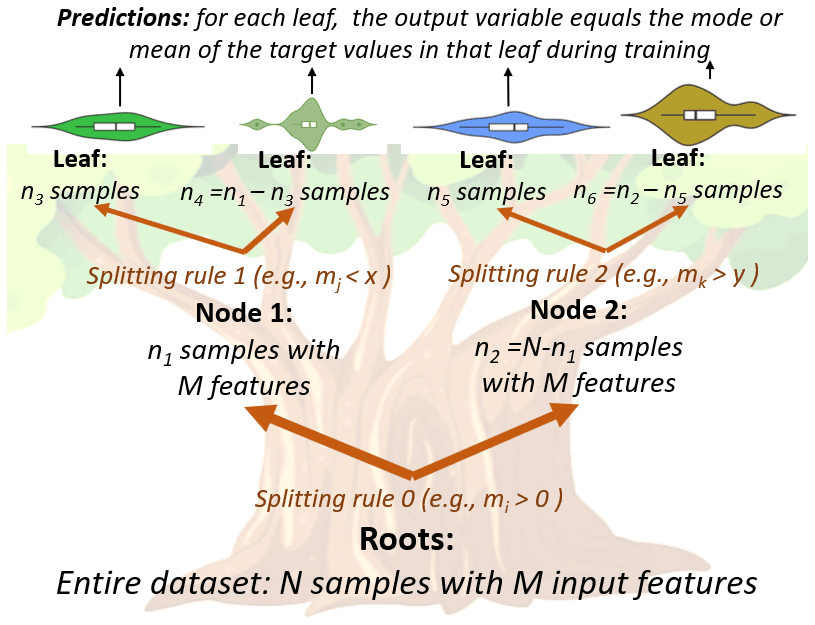
Figure 1 Example structure of a decision tree for a given dataset with N samples and M features, having seven nodes in total: one root node, two decision nodes, and four leaves, resulting in an overall depth of three (i.e., longest path from roots to leaves).

3 Study area and data

The study area includes most of northern Italy and a little part of Switzerland, with a total extent of about 10⁵ km². Many different geographical subsystems can be found within this surface: the Alps, located in the north, occupy about 5×10⁴ km², with an average elevation of 2500 m a.s.l. and mainly rocky soil. This mountain range also hosts several big lakes, such as Lake Garda, Lake Maggiore, and Lake Iseo. The Apennines, in the southern portion, have lower altitudes than the Alps and more permeable soils. The Po Valley, the largest floodplain in Italy, stretches from west to east, covering an area of about 4.6×10⁴ km², going from the Alps and the Apennines to the Adriatic Sea (see Fig. 2). The study area is mostly occupied by the Po river basin, which is the largest in Italy. Moreover, other important rivers are the Adige, Brenta, Reno, and Bacchiglione. For this large and predominantly flat region, floods represent a major issue, also considering its high population density and presence of strategic industrial and agricultural assets (ISPRA, 2018; Persiano et al., 2020).

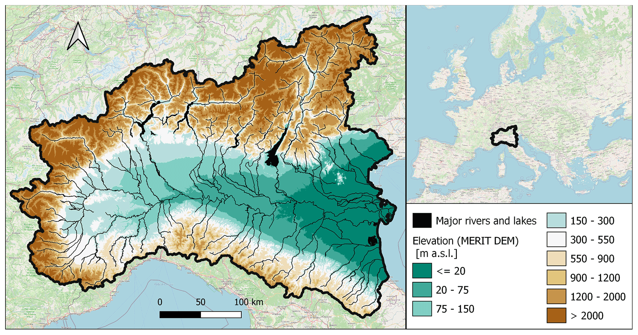
Figure 2 MERIT DEM for the study area, with major rivers and lakes marked in black (left); study area in the European context (right; map from © OpenStreetMap contributors, 2017, distributed under the Open Data Commons Open Database License (ODbL), v1.0).

The DEM used to represent the study area is the freely available Multi-Error-Remover Improved-Terrain model (MERIT; see Yamazaki et al., 2017). This choice was made for two reasons. First, MERIT should be quite reliable for hydrological applications as it is the product of several processing operations and corrections on previously available DEMs (i.e., NASA SRTM3 and JAXA AW3D), some of which specifically address hydrological consistency (e.g., agreement between modelled and real stream network). The second reason is that its resolution is 3 arcsec, which corresponds to ∼90 m at the Equator. These characteristics enabled us to perform an accurate computation of geomorphic indices while reducing the computational costs.

Two different freely available reference flood hazard maps have been used to train the ML models. The first, used for the classification problem (i.e., delineation of flood extent), has been produced by the Italian Institute for Environmental Protection and Research (ISPRA) to fulfil the Floods Directive of the European Parliament (2007/60/EC). This map (hereinafter referred to as PGRA P1) refers to a return period of about 500 years and comes from the merge of different hazard maps produced by local authorities, which explains its heterogeneity. Detailed flood hazard mapping characterizes some areas (e.g., see the north-western portion of the study area in Fig. 3), while lacking information affects other zones (e.g., see the north-eastern portion of the study area in Fig. 3). In the reminder of this study we term exhaustiveness the degree of detail to which flood hazard is defined and captured for minor streams. The second map (see Fig. 4), used for the regression problem (i.e., estimation of water depth), is made available by the study from the Joint Research Centre (JRC) of the European Commission and refers to a return period of 100 years; it is referred to as JRC 100 in the remainder of the study. Differently from PGRA P1, JRC 100 provides information in terms of water depth and is uniform throughout the study area, yet evenly incomplete and less accurate for minor streams as it comes from the merger of several numerical simulations which considered only river catchments with drainage area higher than 500 km² (see Dottori et al., 2016).

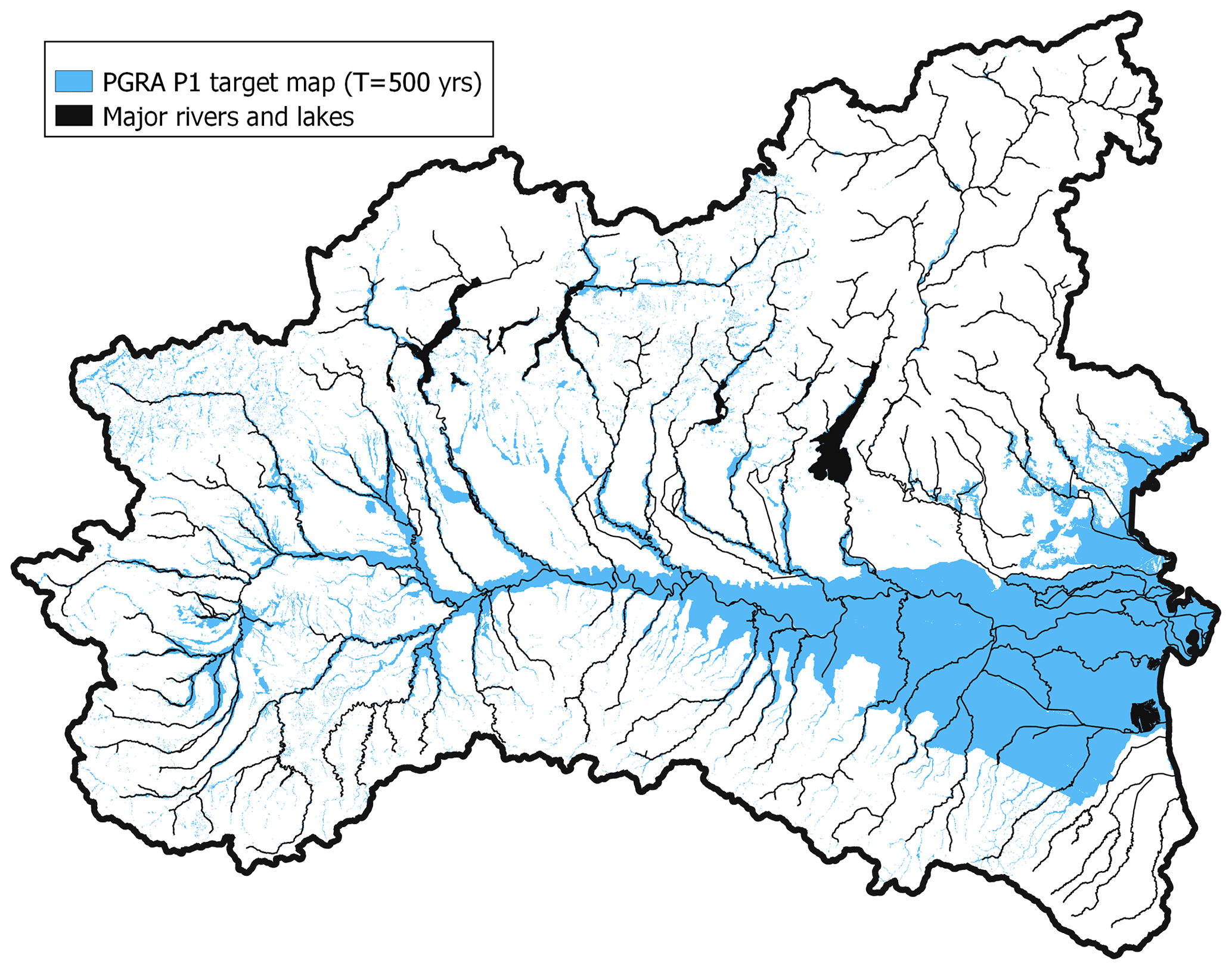
Figure 3 Binary flood hazard target map with return period ∼ 500 years, made available by ISPRA and termed PGRA P1 in this study.

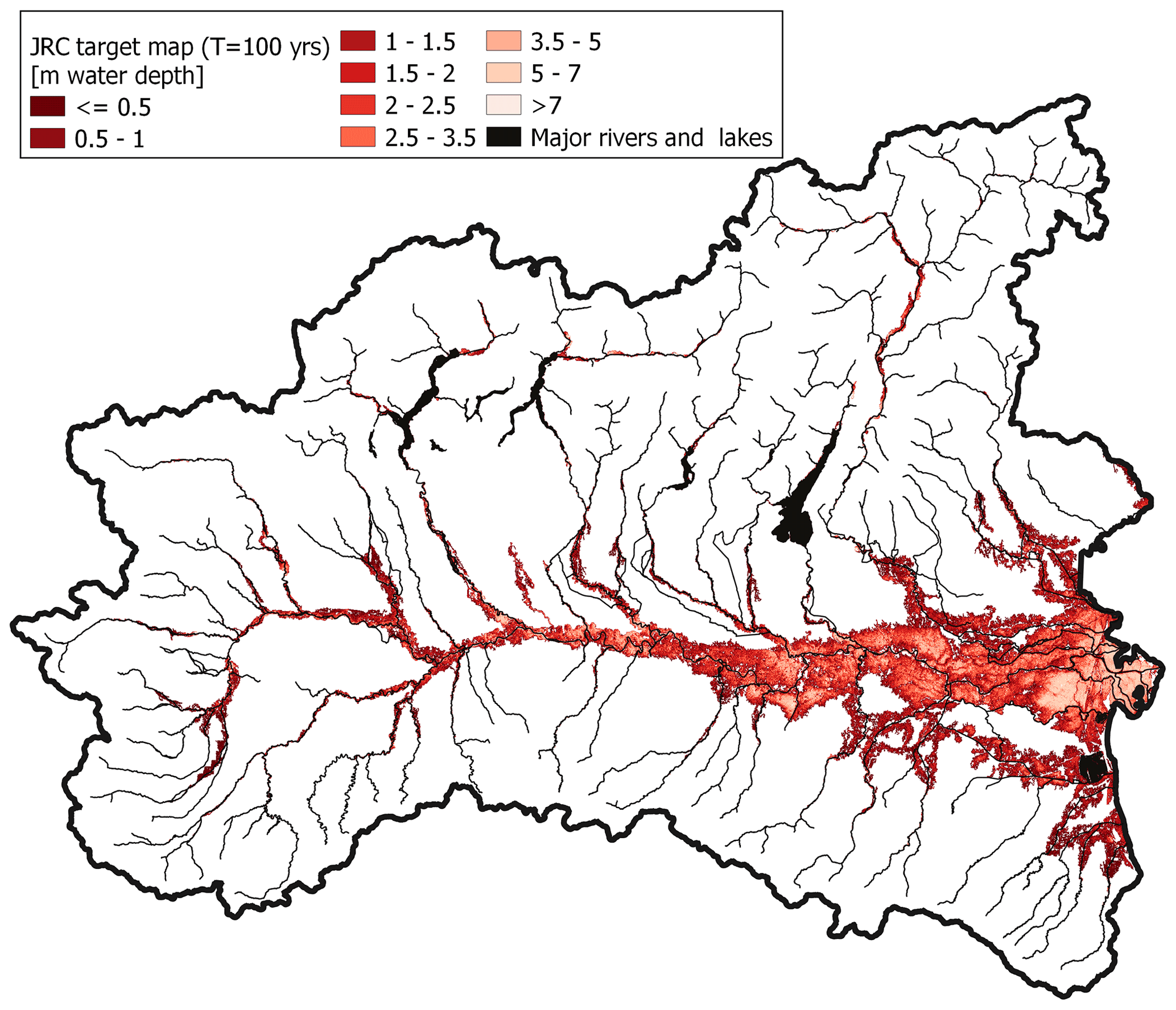
Figure 4 Water depth for the target 100-year flood hazard map obtained by Dottori et al. (2016), termed JRC 100 in this study (colour classes in the legend are used for data visualization only).

4 Framework of the analysis

This section provides an overview of the four macro-phases of the present study.

1. Data selection and preparation:

   • a.

     selection of the DEM and computation of geomorphic indices with terrain analysis

   • b.

     selection of the flood hazard target map

2. Preliminary analyses:

   • a.

     definition and preparation of the calibration area

   • b.

     selection of performance metrics and objective functions

3. Implementation of the univariate approach (benchmark approach): set-up of GFI optimal threshold in randomly selected 85 % of calibration area

4. Testing multivariate approach with two different modes (a and b):

   • a.

     geographical interpolation – the training set consisting of randomly selected 85 % of calibration area, the testing set consisting of randomly selected 15 % of calibration area

   • b.

     geographical extrapolation – the training set consisting of a geographical subregion of the calibration area, the testing set consisting of the geographical remainder of the calibration area

Macro-phase 1 of the study consists of the preparation of input data, which is a fundamental step for the success of machine-learning algorithms; specific criteria are used to select the GDs (Sect. 2.1), the accuracy and horizontal resolution of the DEM, and the target flood hazard datasets (Sect. 3). Phase 2 (i.e., preliminary analyses) is necessary for defining some important aspects for the successful set-up of DEM-based models: the calibration area (Sect. 4.1), the objective functions, and the performance metrics for evaluating the results (Sect. 4.2). Phase 3 identifies the benchmarking approach, i.e., a univariate DEM-based model for classification of flood-susceptible areas to be used as comparison for the successive analysis. This model is built up according to the indications reported in the literature and considers the GFI descriptor alone as it is found to be the most versatile and accurate by many authors (e.g., Samela et al., 2017).

The main results of the study are obtained in phase 4 as the DEM-based multivariate approach is tested in two different ways. First, two DTs are set up (i.e., one classifier DT and one regressor DT) using training and test sets with the same statistical distribution of input features. This represents an ideal case (here termed geographical interpolation mode), in which the training and test sets have very similar morphoclimatic characteristics. Second, four sub-portions of the study area are selected based on specific morphoclimatic conditions, and then, eight more DTs are trained on these areas (i.e., one classifier DT and one regressor DT for each training area) and tested on the complement to the study region (see Sect. 4.3). This represents a data-scarce case (here termed geographical extrapolation mode), in which morphoclimatic characteristics of training and test sets may be rather different.

4.1 Calibration area

Previous studies (e.g., Tavares da Costa et al., 2019) have highlighted that the DEM-based classification of regions into flood-prone and flood-free zones is more effective if the calibration is done on meaningful areas. This is due to the different importance of far-from-river and close-to-river pixels in the computation of the objective function. In the present study, training and testing of the models have been performed referring to a portion of the entire study area, which we term calibration area. Different methods to define this area have been tested during the preliminary analyses of phase 2, finding that the most effective way, representing a good trade-off between the calibration efficiency and the ease of identification, is to refer to a constant-radius buffer around the target flood hazard map. In particular, based on sensitivity analyses that clearly showed that the radius value has a non-negligible impact on the accuracy of the trained model, a 2 km radius has been selected for the PGRA P1 target map and a 5 km radius for the JRC 100 map (see Fig. 5). During our analyses, all the pixels falling outside the 2 and 5 km calibration buffer areas are neglected when fitting the models and evaluating the results for all classification and regression problems, respectively.

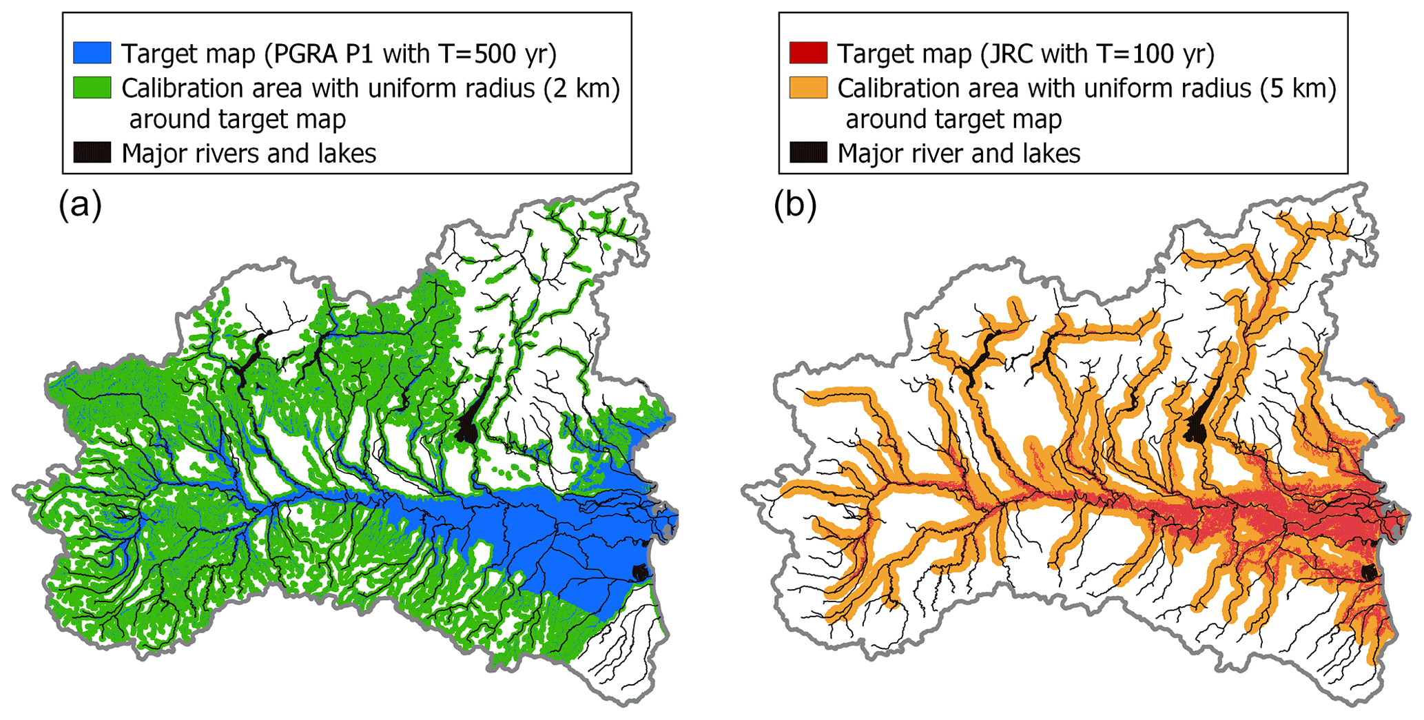
Figure 5 Calibration areas: 2 km buffer (green) and PGRA P1 flood-prone areas (blue) used for the classification problem (a); 5 km buffer (orange) and JRC 100 flood-prone areas (red) used for the regression problem (b).

4.2 Objective functions and performance metrics

Specific objective functions are used to train the DTs for classification and regression, while other performance metrics are computed to evaluate their predictions during the validation. With regards to the classification problem, the objective function, used during the training of the DTs to assess the quality of each split, is the Gini impurity (I_G(p)), which varies between 0 (the optimal value) and 1 (Hastie et al., 2009). At each step, the Gini impurity measures how often a randomly chosen element from the set would be incorrectly labelled if it was randomly labelled according to the distribution in the subset. Given the number of target classes J and the fraction of items labelled with class i in the set p_i, the Gini impurity is defined as follows:

$$\begin{array}{}\text{(4)}& I_{\mathrm{G}}\left(p\right)=\sum _{i=\mathrm{1}}^J{p}_i\times (\mathrm{1}-p_i).\end{array}$$

To perform implementation of the univariate approach, parameterize the multivariate classifier DTs, and evaluate the results, we use the true skill statistic (TSS; Youden, 1950; Everitt et al., 2002), which is based on the contingency matrix and varies between 0 and 1 (optimal value):

$$\begin{array}{}\text{(5)}& \mathrm{TSS}={\displaystyle \frac{\mathrm{TP}}{\mathrm{TP}+\mathrm{FN}}}+{\displaystyle \frac{\mathrm{TN}}{\mathrm{TN}+\mathrm{FP}}}-\mathrm{1},\end{array}$$

where TP, TN, FP, and FN are true positive, true negative, false positive, and false negative predictions of the model, respectively. TSS has been successfully used by several authors in different applications (Bartholmes et al., 2009; Alfieri et al., 2012; Tavares da Costa et al., 2019). During preliminary analyses of phase 2, some experiments suggested preferring this metric to accuracy (ACC; see below), which was shown to be less sensitive to model modifications (i.e., different calibration areas, input information, tree depth) and goodness (lower extension of FP and FN areas).

Other metrics used for analysing the results are accuracy (ACC), precision (or positive predictive value, PPV), and recall (or true positive ratio, TPR). All three are very common in evaluating the performance of a classifier (e.g., Manfreda et al., 2015; Samela et al., 2017). They all vary between 0 and 1 (optimal value) and are defined as follows:

$$\begin{array}{}\text{(6)}& {\displaystyle }\mathrm{ACC}={\displaystyle \frac{\mathrm{TP}+\mathrm{TN}}{\mathrm{TP}+\mathrm{TN}+\mathrm{FP}+\mathrm{FN}}}\text{(7)}& {\displaystyle }\mathrm{PPV}={\displaystyle \frac{\mathrm{TP}}{\mathrm{TP}+\mathrm{FP}}}\text{(8)}& {\displaystyle }\mathrm{TPR}={\displaystyle \frac{\mathrm{TP}}{\mathrm{TP}+\mathrm{FN}}}.\end{array}$$

With regards to the regression problem, the objective function to minimize during the training is the well-established mean square error (MSE). Using n, $\widehat{y_i}$, and y_i to indicate the number of samples and the predicted and target value, respectively, MSE can be written as

$$\begin{array}{}\text{(9)}& \mathrm{MSE}={\displaystyle \frac{\mathrm{1}}{n}}\sum _{i=\mathrm{1}}^n{\left(y_i-\widehat{y_i}\right)}^{\mathrm{2}}.\end{array}$$

The metric mainly used to evaluate the results and parameterize the multivariate regressor DTs is the determination coefficient R², which varies between −∞ and 1 (the optimal value). It measures the improvement of the predicted values relative to the mean of the input samples ($\stackrel{\mathrm{‾}}{y}$), defined as

$$\begin{array}{}\text{(10)}& R^{\mathrm{2}}=\mathrm{1}-{\displaystyle \frac{{\sum }_{i=\mathrm{1}}^n{\left(y_i-\widehat{y_i}\right)}^{\mathrm{2}}}{{\sum }_{i=\mathrm{1}}^n{\left(y_i-\stackrel{\mathrm{‾}}{y}\right)}^{\mathrm{2}}}}.\end{array}$$

The last considered metric is the mean absolute error (MAE), defined as

$$\begin{array}{}\text{(11)}& \mathrm{MAE}={\displaystyle \frac{\mathrm{1}}{n}}\sum _{i=\mathrm{1}}^n|y_i-\widehat{y_i}|.\end{array}$$

Lastly, we used the Gini importance (GI) to measure the importance of each factor (i.e., each GD) in the trained models (both classifier and regressor DTs), which is defined for the jth factor as follows:

$$\begin{array}{}\text{(12)}& {\mathrm{GI}}_j={\displaystyle \frac{{\sum }_{i=\mathrm{1}}^{N_j}{I}_{G_i}\cdot \left(n_i\right)-I_{G_{i,\mathrm{r}}}\cdot \left(n_{i,\mathrm{r}}\right)-I_{G_{i,\mathrm{l}}}\cdot \left(n_{i,\mathrm{l}}\right)}{{\sum }_{i=\mathrm{1}}^N{I}_{G_i}\cdot \left(n_i\right)-I_{G_{i,\mathrm{r}}}\cdot \left(n_{i,\mathrm{r}}\right)-I_{G_{i,\mathrm{l}}}\cdot \left(n_{i,\mathrm{l}}\right)}},\end{array}$$

where $I_{G_i}$, $I_{G_{i,\mathrm{r}}}$, and $I_{G_{i,\mathrm{l}}}$ are respectively the impurities of node i and its right and left child nodes; n_i, n_i,r, and n_i,l are the fractions of samples reaching the corresponding nodes; N_j is the number of nodes where a condition on the jth factor is used as a splitting rule; and N is the total number of nodes. Although this measure is largely used for its speed of computation, it has the drawback of neglecting the weakest factor when two related factors are used, which has to be taken into account when discussing the results.

4.3 Training and testing strategy

All models considered in this study are trained and tested in different sub-domains of their calibration area based on two different strategies. For the univariate model and the interpolation DTs, the pixels of the calibration area have been randomly split, with 85 % going to the training and 15 % to the test set, based on the established proportion adopted for machine-learning algorithms (Mosavi et al., 2018). This produces two datasets with millions of pixels, both with very diverse ranges of input and target information. During the extrapolation analyses, training is performed in turn on four different portions of the overall calibration area. To avoid dividing any catchment into a part for training and one for testing, the delineation of these areas follows catchment boundaries as well as precise geographical and hydrological criteria (see Fig. 6):

• Area A includes the Alpine catchments and the northern portion of the Po river floodplain. The complementary test area includes all the Apennines, a lower mountain range, and the southern part of the Po plain, where smaller river catchments are located.

• Area B includes catchments in the upstream sector of the Po river basin, representing part of the Alps and of the Apennines. The complementary test area includes most of the Po plain and part of the Alps and Apennines.

• Area C is complementary to area B and consists of the downstream portion of the Po river basin.

• Area D includes the Apennines, western and central Alps, and the entire Po streamline. Its complementary test area contains a rather small part of the Po plain; the western Alps; and the flood plain of the Adige, Brenta, and Bacchiglione rivers.

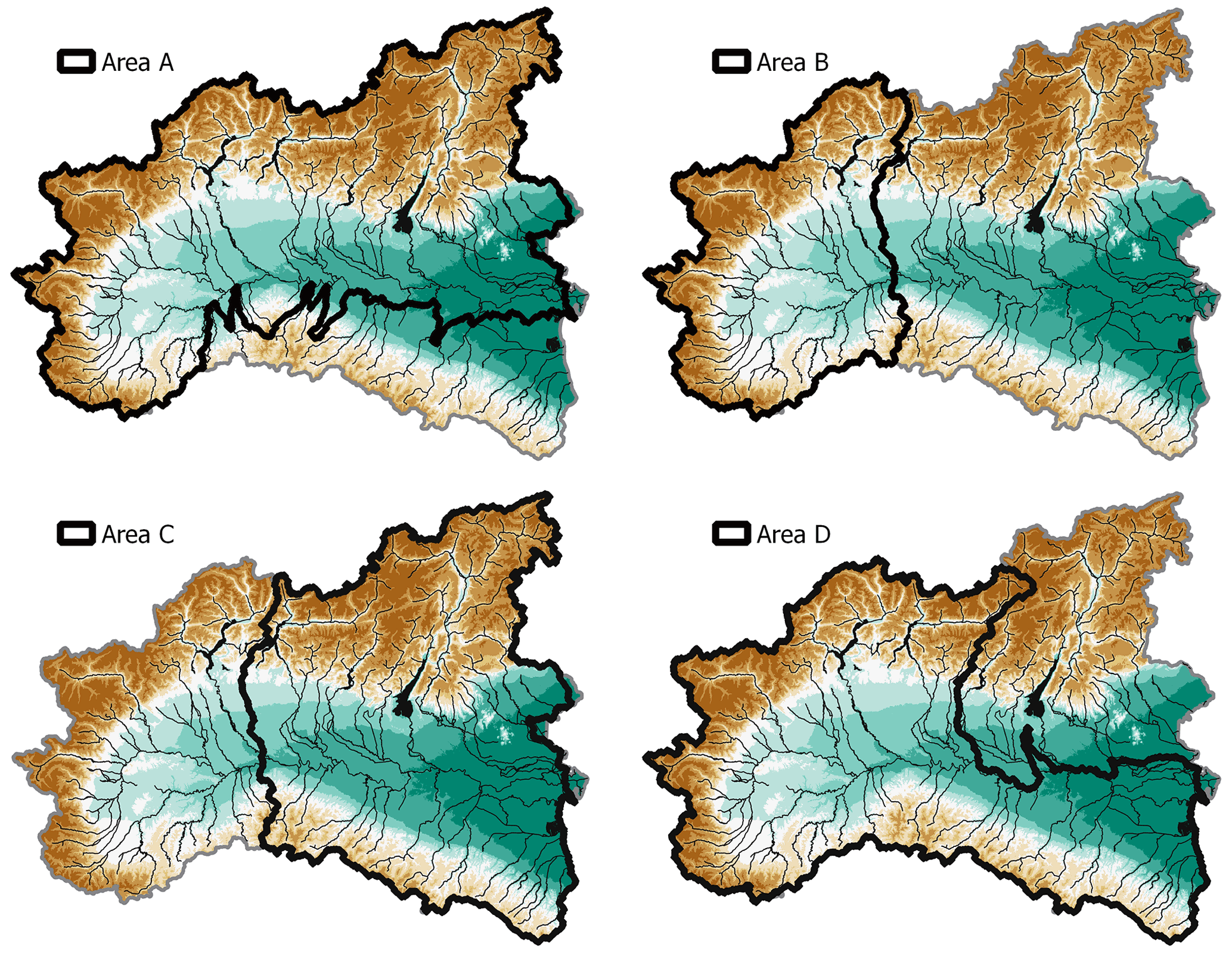
Figure 6 Training areas (bold contour) used for the geographical extrapolation experiments performed in phase 4, with major rivers and lakes highlighted in black.

Before training DTs, k-fold cross-validation (CV) is performed to optimize models' hyper-parameters, namely the maximum tree depth and the minimum number of records in any leaf node; k-fold CV is a widely used method for model parameterization and selection (Hastie et al., 2009) and consists of dividing the training set into k folds and then performing two consecutive operations: (1) training of the model using k−1 folds and (2) validation of the model using the remaining fold. These two steps are repeated k times for all the combinations of the k folds of the training data.

5 Results

The reliability of the predictions of the models is assessed by performance metrics that refer to (a) the training set and (b) the test set. While the metrics computed for the training set assess the reliability in reproducing the observed target map, the ones regarding the test set measure the ability of the model when applied to a different sample than the one used in training (i.e., validation of the model). In order to find out the relevance of each input GD in the DTs’ structure, the Gini importance (see Sect. 4.2) for each model is reported in Table 3 and is discussed in more detail in Sect. 6.

5.1 Delineation of flood-prone areas in interpolation mode

Figure 7 represents the flood susceptibility map obtained with the classifier DT model trained within the random 85 % of the 2 km buffer calibration area (i.e., multivariate flood susceptibility map). To understand the quality of the proposed approach and profitably discuss the results, Fig. 8 illustrates the map produced with the univariate benchmark approach set up in the same area. Relevant performance metrics for multivariate and univariate models are reported in rows 1 and 2 of Table 1, respectively.

Figure 7 and Table 1 highlight that the DT flood susceptibility map is strongly consistent with the target map PGRA P1. Also, the model produces a rather detailed mapping across floodplains of minor streams (i.e.,  exhaustiveness, as defined in Sect. 3); in particular, it can be observed in Fig. 7 that the zones where the target map has high exhaustiveness (e.g., north-western portion of the study area) are mapped with slightly lower exhaustiveness by the DT model, while the DT output is more detailed in the floodplain of minor streams than the target map, where the latter is lacking exhaustiveness (e.g., north-eastern part).

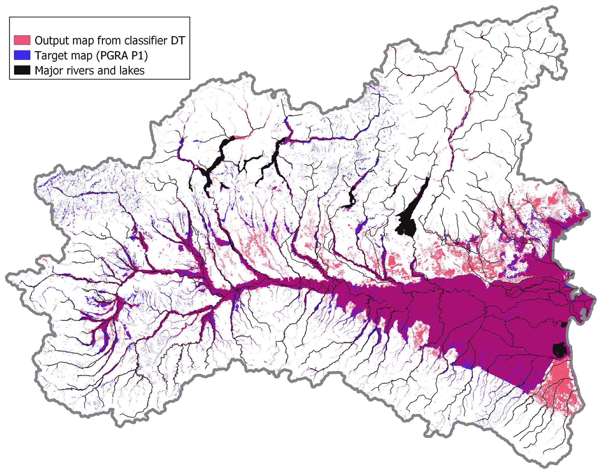
Figure 7 Multivariate 500-year flood susceptibility map for the study area (red), target flood hazard map (PGRA P1; blue). Purple indicates overlaying areas.

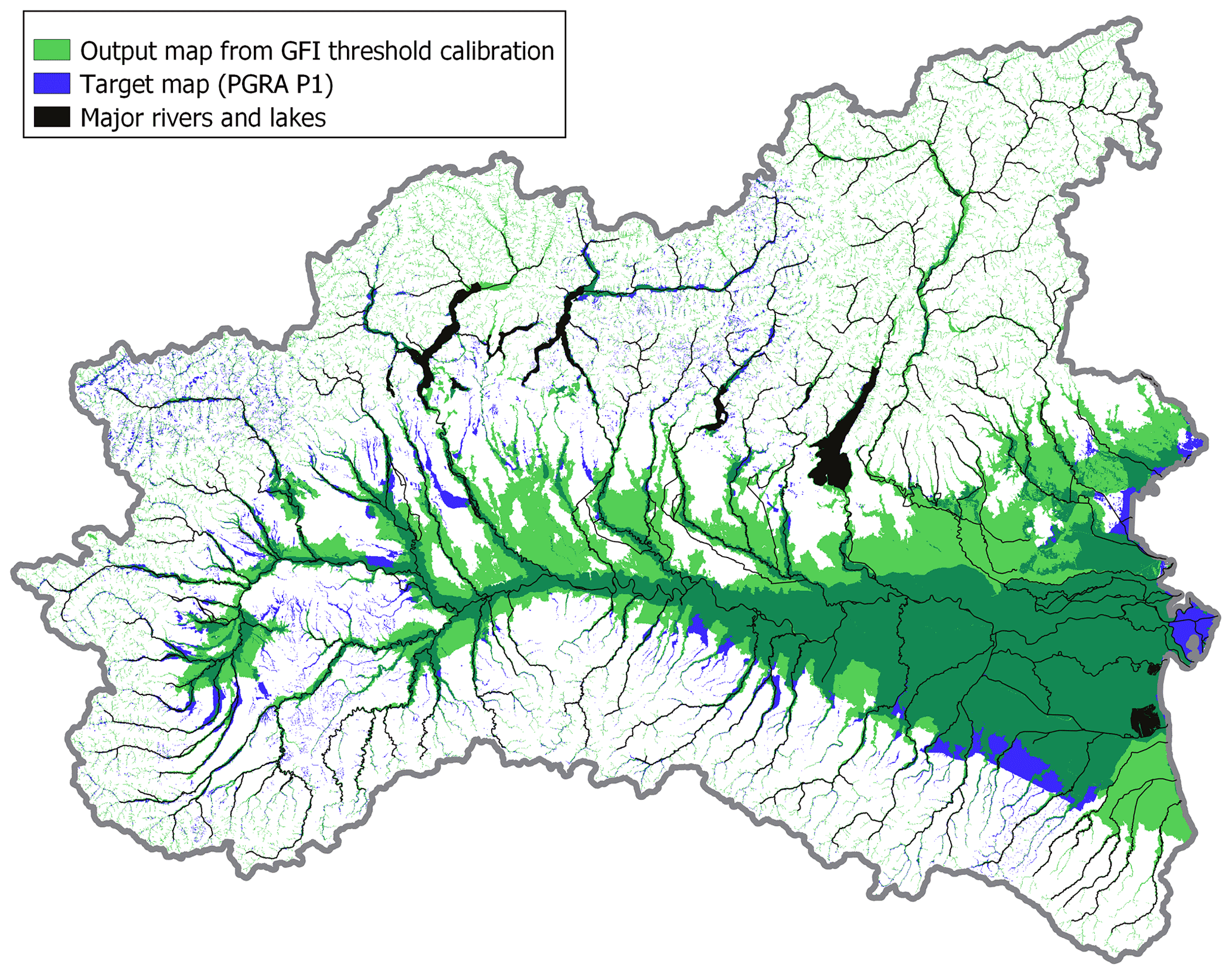
Figure 8 Binary flood susceptibility map resulting from a univariate analysis (morphometric index: GFI; light green), target flood hazard map (PGRA P1; blue). Dark green indicates overlaying areas.

Table 1 Classification problem: performance metrics for the multivariate (classifier DTs) and univariate (classifier GFI) flood susceptibility maps; target flood hazard map for both approaches: PGRA P1. The reported values have been converted from the interval 0−1 to the percentage notation. The best testing metric values are reported in bold, the worst ones in italic (the first line should be compared with the second one; the last four lines should be compared to each other).

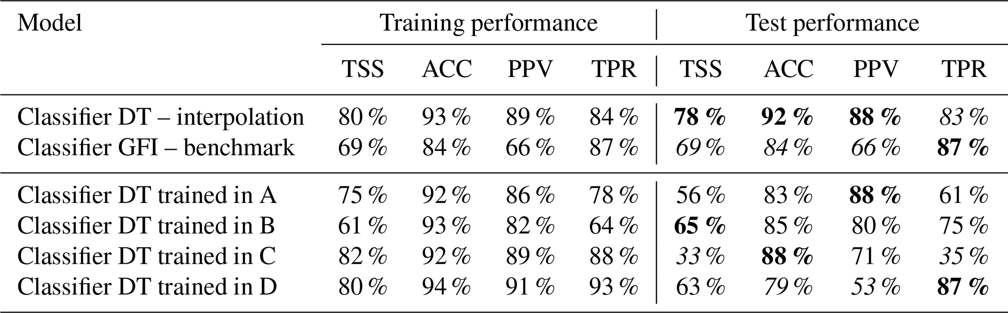
Figure 7 shows that GFI uniformly and exhaustively estimates flood susceptibility along all minor streams in mountain areas but tends to severely overestimate the size of flood-prone areas in predominantly flat regions.

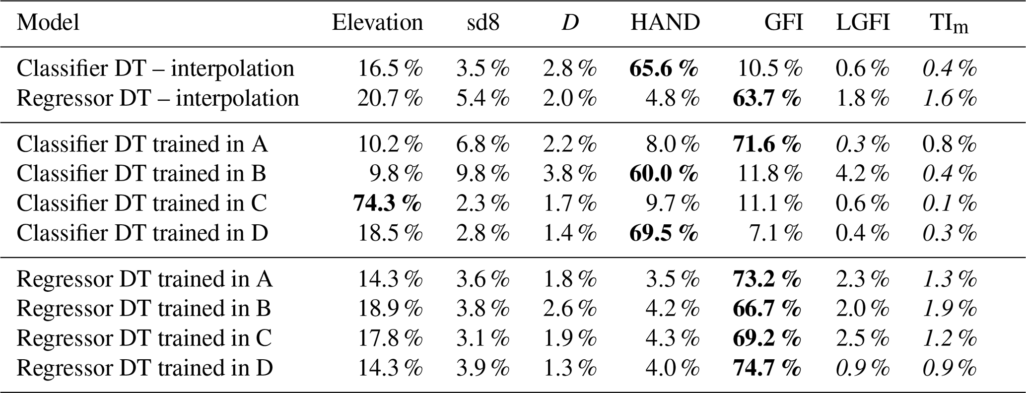
The first line of Table 3 reports the Gini importance for the classifier DT: HAND scores about 65 %, followed by elevation (16.5 %) and GFI (10.5 %).

5.2 Prediction of flood hazard intensity in interpolation mode

Figure 9 illustrates expected maximum inundation water depths as predicted through the regressor DT trained within the random 85 % of the 5 km buffer calibration area; relevant performance metrics can be found in the first row of Table 2. Figure 9 and Table 2 show good performance of the DT model for the regression problem. It is worth noting here that the exhaustiveness of the DT water depth map is considerably higher than that of the reference map (i.e., JRC 100). This result was expected due to the focus of JRC 100 on larger catchments.

The data density plot in Fig. 10 depicts the relationship between target and predicted water depths for the test set focusing on true positives (i.e., both target and predicted water depths are higher than 0.0 m) and neglecting water depths higher than 3.5 m (neglected pairs, beyond axes' limits, are 4.2 % of the total).

The second row of Table 3 shows that the most informative GD is GFI (63.7 %), followed by elevation (20.7 %) and slope (5.4 %).

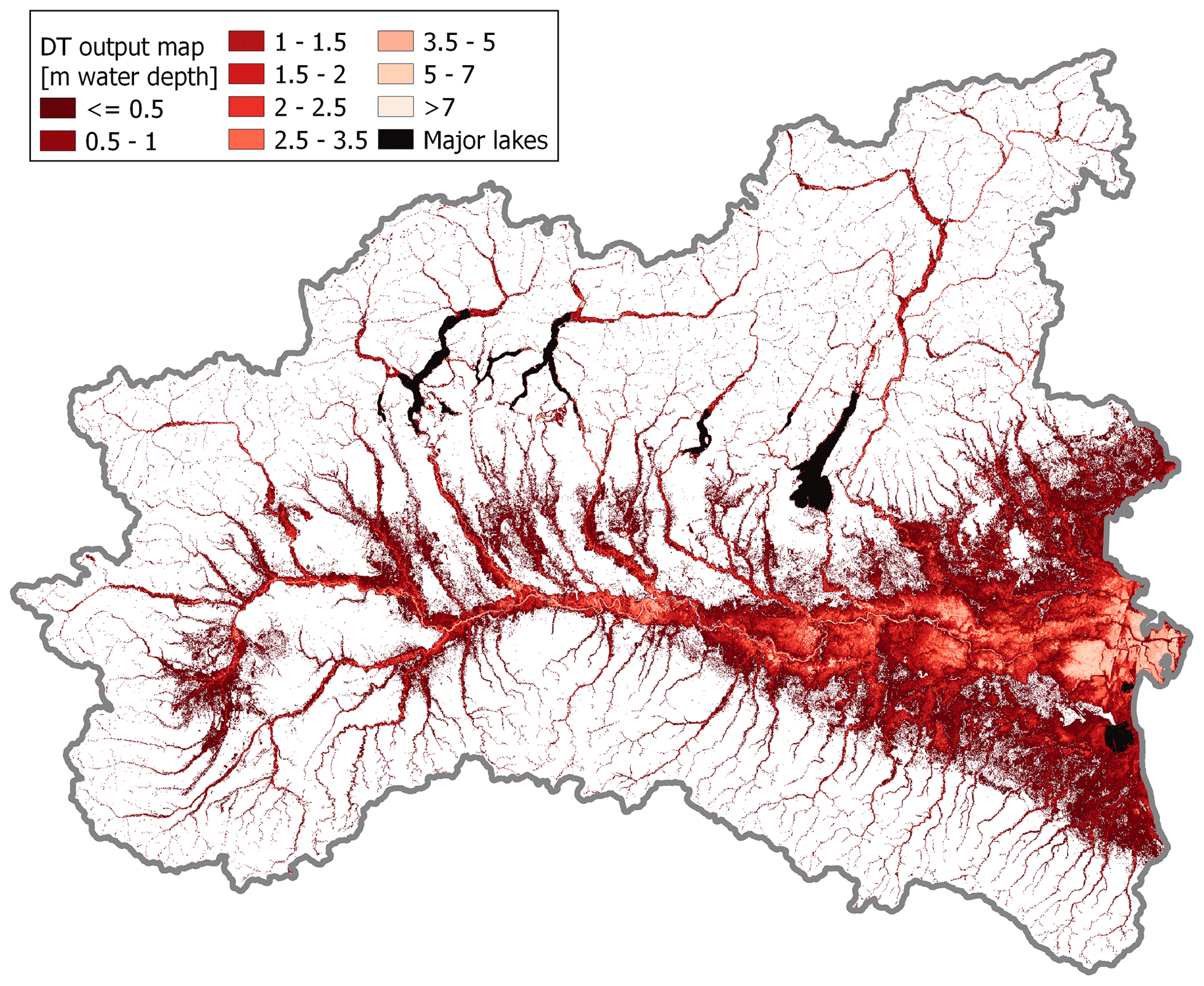
Figure 9 Multivariate water depth hazard map obtained with regressor DT in interpolation mode (target flood hazard map: JRC 100).

Figure 10 Data density plot (%) for target vs. predicted expected maximum water depth (target values: empirical JRC 100; predicted values: regressor DT applied to the test set).

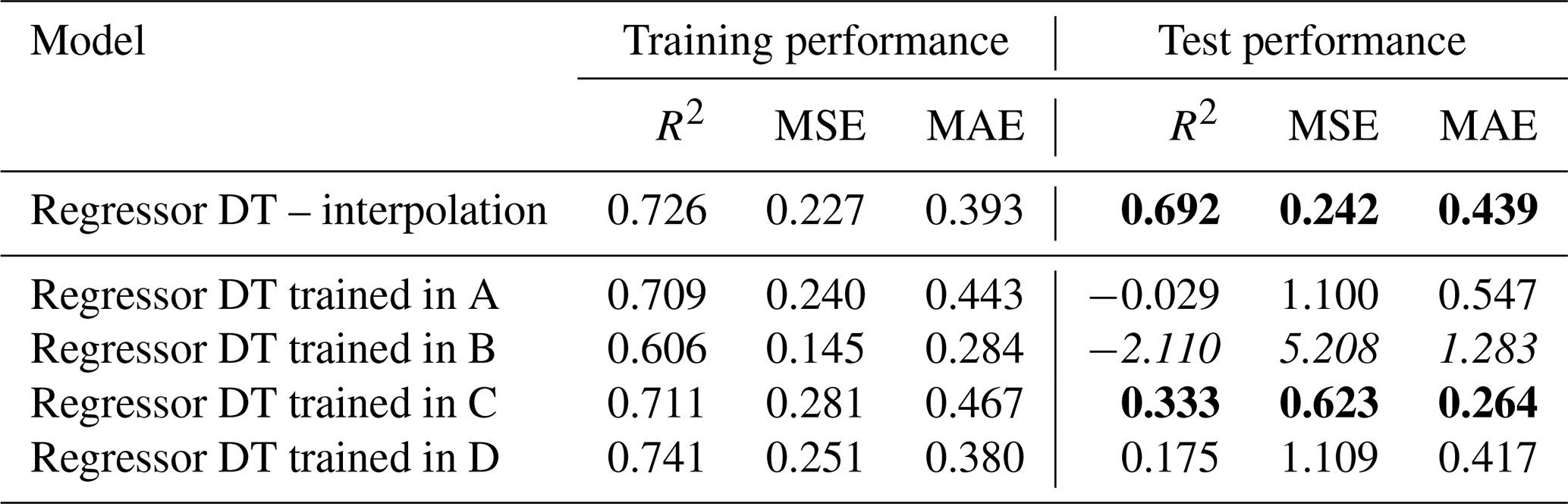
Table 2 Regression problem: performance metrics for the multivariate water depth output maps obtained with the regressor DTs (target flood hazard map: JRC 100); the best testing metrics values are reported in bold, the worst ones in italics.

5.3 Multivariate flood hazard modelling in extrapolation mode

Tables 1 (rows 3–6) and 2 (rows 2–5) report performance metrics for the geographical extrapolation experiments for the classification and regression problems, respectively, while Figs. 11 and 12 depict the corresponding DT output maps.

With regards to the classification problem (Table 1), the performance metrics highlight a generalized good agreement with the target map. Figure 11 and the “Training performance” column of Table 1 show that all models can accurately reproduce the target map in the training area, but they are quite inaccurate in the test area as the difference between the two is evident. In fact, concerning the test area, Table 1 shows that according to the true skill score (TSS), the best prediction in the test area is obtained using B as the training area (TSS =65 %), followed by D (TSS =63 %) and A (TSS =56 %), respectively. The same table section shows that the best results are obtained when training on area C if one focuses on accuracy (ACC =88 %), followed by B (ACC =85 %) and A (ACC =83 %). According to precision (PPV), the best result is obtained by training the model on area A (PPV =88 %), while it is D according to recall (TPR =87 %).

Concerning the regression problem, worse predictive skill in geographical extrapolation is observed in Table 2. Differently from the classification, performance metrics for the regression problem are in good agreement among each other, showing that area C has the better results, while area B is the worst. On the other hand, Fig. 12 suggests that water depth estimation in the test area is quite reliable in all the cases, with the exception of the DT trained in area B.

Focusing on Gini importance, Table 3 clearly shows that regressor DTs (rows 7–10) are characterized by similar structures regardless of the training areas: GFI is always ranked first in terms of relevance, followed by elevation and slope. This is not true for the classification problem (rows 3–6): in this case, classifier DTs identified four different training areas that have different structures, in which the most informative geomorphic descriptor can alternatively be GFI, HAND, or the elevation; the latter is always ranked second.

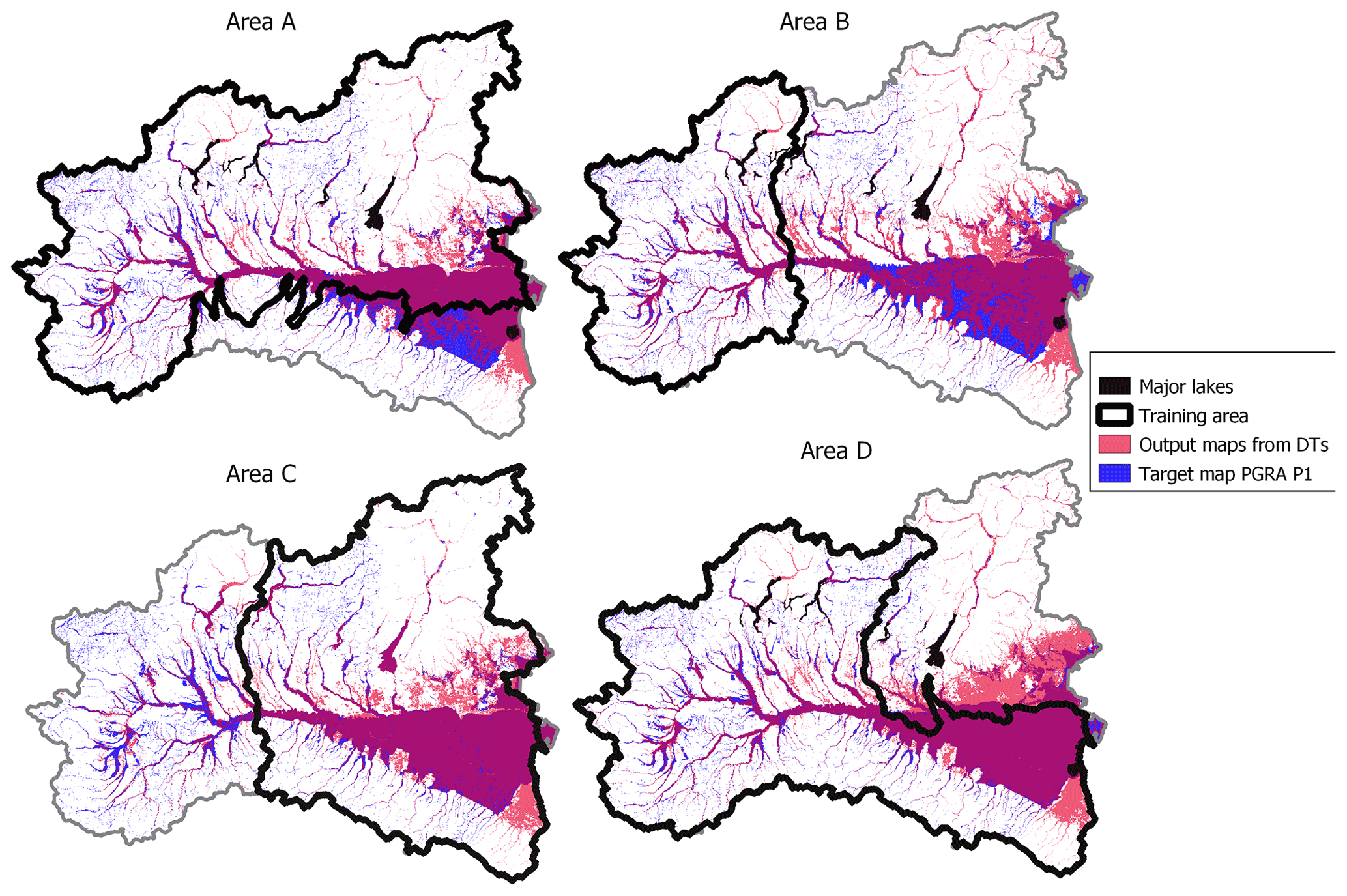
Figure 11 Geographical extrapolation for the classification problem: multivariate flood susceptibility maps obtained from classifier DTs (red), target flood hazard map (PGRA P1; blue). Purple indicates overlaying areas.

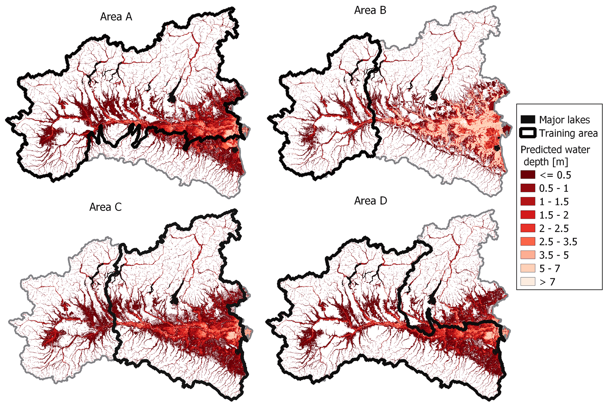
Figure 12 Geographical extrapolation for the regression problem: multivariate flood susceptibility maps obtained from regressor DTs (see also Fig. 4; target flood hazard map: JRC 100).

Table 3 Gini importance of the selected input features computed for the DTs trained in phase 4; the highest value for each DT is highlighted in bold, the lowest in italic.

6 Discussion

6.1 Can we profit from a blend of various geomorphic descriptors for flood hazard assessment and mapping?

The first goal of the present research is the evaluation of the improvement which can be obtained by applying a machine-learning-aided, multivariate, DEM-based flood hazard assessment relative to a univariate DEM-based approach. First, regarding the classification problem (i.e., differentiation between flood-prone and flood-free areas), the outcomes reported in Figs. 7–8 and Table 1 (rows 1–2) suggest that the combination of multiple geomorphic descriptors (GDs) increases the comprehensiveness of the morphological description of the study area, and the resulting multivariate data-driven model can reproduce the reference flood hazard map in a significantly enhanced way relative to a univariate approach adopting a single GD. This is particularly visible from the lower extension of wrongly predicted areas (i.e., false positive, or FP, and false negative, or FN) in the classifier DT output map (light-red and blue areas in Fig. 7) relative to the GFI output map (light-green and blue areas in Fig. 8).

Second, concerning the regression problem (i.e., prediction of the flood intensity, such as the expected maximum water depth associated with a given probability of occurrence) the regressor DT considered for interpolation shows high accuracy in reproducing the target map. Also, it is worth highlighting that regressor DTs provide a direct estimate of this variable relative to the traditional univariate DEM-based approaches, which usually require the prior delineation of flood extent to compute water depth, as the elevation difference between the flood-extent border and each pixel (see Manfreda and Samela, 2019). Figure 10 highlights that the correlation between the predicted and target water depths can be improved, yet it also clearly shows that predictions for the test set are unbiased. It is worth mentioning here that the diagram neglects the true negatives (i.e., target and predicted water depths are equal to 0.0 m; 49.78 % of the cases), false positives (i.e.,  only predicted water depths are equal to 0.0 m; 22.37 % of the cases), and false negatives (i.e., only target water depths are equal to 0.0 m; 0.08 % of the cases). While the occurrence of the most concerning cases (false negatives) is very limited, predictions show significant margins for improvement as far as the false positives are concerned. Nevertheless, it should also be recalled here that the target map by its own very nature neglects smaller streams (contributing area has to be higher than 500 km²), whereas the decision tree regressor looks at morphology only and provides water depth predictions also for smaller streams (i.e., higher exhaustiveness; see Fig. 9).

One of the most interesting aspects is the relevance that each GD assumes in the regressor DTs (see Table 3). It can be observed that all models rely mainly on one single GD, with Gini importance always in excess of 60 %, but still, the multivariate analysis leads to significantly better results relative to the univariate one. Also, it is important to highlight that

• while regressor DTs tend to depend mainly on the GFI, classifier DTs depend on HAND;

• while the input GDs have quite a similar Gini importance hierarchy in regressor DTs, classifier DTs assume different hierarchical structures depending on the considered training area;

• all models agree on giving low Gini importance to LGFI and TI_m, probably due to redundant information relative to the GFI;

• elevation is very often ranked second and always associated with significant importance.

Overall, this suggests that regressor DTs tend to operate by correcting a baseline estimate that mostly relies on the GFI value. On the other hand, classifier DTs obtain their results by following different rules depending on the training data and often prefer using lower-level features relative to more complex indicators such as the GFI. This sensitivity to the training area makes it difficult to set a priori weights to the GDs when building up the models. It should be kept in mind, however, that different Gini importance values do not necessarily imply radically different classification rules due to the existing correlations between the input features. Ideally, dedicated feature selection and importance analysis algorithms should be used to obtain deeper insight on how the different models come to their conclusions; we plan to investigate this line as part of future work.

6.2 Can we use simple ML techniques for effectively blending multiple GDs?

The second research question of the present study is whether it is possible to obtain a good estimation of flood hazard by combining multiple GDs with low-complexity machine-learning models. Differently from several other contributions in the literature, we do not focus on model complexity nor on the comparison of different models (Wang et al., 2015; Khosravi et al., 2018; Mosavi et al., 2018; Arabameri et al., 2019; Costache et al., 2020). Instead, we prefer to select one simple model type (i.e., decision trees, DTs) and focus on the combination of the five innovative elements listed in the “Introduction” section; in this way, we can analyse the influence on the multivariate DEM-based approach of the preliminary steps, consisting of data pre-processing (i.e., selection and manipulation of input features, target maps, training set, and test set). This is highly important because machine-learning models do not reproduce the dynamics of the water; as such, their performance is strictly linked to the data used for the training, which need to be handled very carefully.

As is highlighted in Sect. 6.1, the outcomes of the study (Figs. 8–9, Tables 1–2) clearly show that DTs can effectively reproduce the target information (Figs. 3–4) with high accuracy for both classification and regression problems, even if the resolution of the MERIT DEM (Yamazaki et al., 2017), from which the input GDs have been retrieved, is not very high. Indeed, even if regressor DTs necessarily implicate discretization of the output variable, in the present study large datasets and appropriate tree depth allow us to obtain wide ranges of different water depth values. Moreover, it is worth mentioning that the trained DTs estimate flood hazard associated with different minor streams that are neglected in the target maps (see red areas in Fig. 7; compare Fig. 9 with Fig. 4): due to the absence of information in these areas, it is not possible to assess the goodness of the models' output, but this tendency of completing target information could be a key aspect for future applications in data-scarce regions, and thus, it could be considered to be a promising characteristic of the models.

Overall, it is possible to observe that DTs are effective tools to combine GDs and estimate flood hazard. This indicates that proper data handling has a strong influence on the accuracy of the final estimation, which is comparable to the choice of a given machine-learning technique. In particular, we want to underline two elements of the presented approach that have great importance on the predictive skill. First, the utilization of flood hazard maps as a target results in a large number of pixels for the training and test set and therefore a very broad spectrum of hydrological and morphological characteristics, which represent a much more informative dataset relative to isolated points used by other authors for training more complex models (Lee et al., 2017; Khosravi et al., 2018; Arabameri et al., 2019; Janizadeh et al., 2019). Second, a sensible identification of a calibration area is very important for successful training as it allows irrelevant pixels to be neglected. To this aim, a preliminary sensitivity analysis might be very useful for identifying the optimal buffering radius around the target map (see Sect. 4.1), even if different approaches are proposed in the literature (e.g., Degiorgis et al., 2012). Indeed, in the case of the application of DEM-based methods in data-scarce areas, where local flood hazard modelling datasets may not be available, global or continental flood hazard maps produced by the European Joint Research Centre (Dottori et al., 2016, 2021) can be used as a target, as done in this study.

6.3 Are these techniques capable of providing a reliable assessment of flood hazard over large areas in extrapolation?

The evaluation of prediction accuracy for geographical extrapolation (i.e., applying the models in geographical areas or watersheds that have not been considered for parameterization and training) is a key and characteristic aspect of our study. On the one hand, performing predictions with new input data is a major problem for machine-learning models; on the other hand, reaching good predictive skills in extrapolation is needed for future practical applications in data-scarce environments. What is more interesting about this part is to understand the link between training and test performances: if the relationship between input and target values, learnt by the model during the training, is also valid for the extrapolation region, accurate test predictions are obtained, but this depends strongly on the choice of input and target datasets for the training, which can be very difficult. Before addressing this very issue, a careful discussion of the resulting metrics and maps is required as their interpretation is not straightforward.

With reference to the classification problem, each metric suggests a different training area as the best case, and this highlights how difficult it is to choose a single metric for describing the goodness of a model for a binary classification. Figure 11 and TSS values in rows 4–5 of Table 2 could suggest that area B (test TSS =65 %) has better extrapolation performance than area C (test TSS =33 %). In contrast, ACC is similar for the two cases and higher for area C (ACC =88 %) than for area B (ACC =85 %), suggesting that TSS is a more informative metric than ACC in representing the model performance. On the other hand, precision and recall appear to be quite unbalanced metrics as areas A and D lead to test prediction with considerable overextension of FN and FP values, respectively (see Fig. 11). Differently, regression metrics agree on pointing at the DT trained in B as the best case (Table 3). However, the absolute values of R², which depicts low-accuracy test predictions, do not reflect other metrics (MSE and MAE) and the output maps (Fig. 12).

As expected, the choice of the training area has great influence on prediction accuracy. This is particularly visible for the classification problem: in Fig. 11, the difference between metrics for the training and test sets is striking. Nevertheless, this difference becomes less clear for the regression problem (Fig. 12). The same observations are confirmed by Table 3, where evidence is given of different structures for the classifier DTs, while the regressor DTs are all very similar. More in detail, the obtained results show that the extent of the training area has less importance than the quality of the input data that it contains. Perfect examples of this remark are classifier DTs trained in A and D: even if both A and D are very wide, prediction over the test area is affected by considerable errors. This happens because A does not include any part of the Apennines, while D ignores a large flat area on the eastern coast, meaning that any geographical system corresponds to a specific relationship between input GDs and flood susceptibility, and thus it cannot be fully represented by a model trained with very different datasets. The comparison between area B and C is also meaningful: while the training in B leads to good test predictions for the classification, it is the worst case for the regression (the opposite is valid for C). This is probably due to the fact that area B contains useful information to delineate flood-prone areas as it represents the upstream section of the Po river but cannot adequately train a regressor DT as it lacks high target values (i.e., high inundation water depths). To sum up, the combination of GDs with DTs is capable of providing quite a reliable estimation of flood hazard (i.e., flood-prone areas and maximum water depth) in extrapolation mode, but a careful choice of the training area is needed, where the target and input dataset is complete and representative of the test area.

7 Conclusions and further steps

Our study analyses and compares data-driven and resource-efficient methods for assessing and mapping riverine flood hazard across large geographical areas. It illustrates the potential and limitations of combining different geomorphic descriptors by means of decision trees for delineating flood-prone areas and for predicting the expected maximum water depths for a given return period. We focus on a large study area in northern Italy (size ∼ 10⁵ km²) containing western, central, and part of the eastern Italian Alps; part of the northern Apennines; and the floodplains of a complex river system including the main rivers Po, Adige, Brenta, Bacchiglione, and Reno. The morphology of the study area is described by the Multi-Error-Remover Improved-Terrain model (MERIT DEM; Yamazaki et al., 2017), with an approximately 90 m resolution. Decision trees are trained using as input features the geomorphic descriptors retrieved from the MERIT DEM and as target maps two different datasets: one representing flood extent with a reference return period of 500 years and one representing expected maximum water depth for a 100-year return period scenario.

Relative to previous studies focusing on morphometric floodplain delineation and flood hazard mapping (see, e.g., Dodov and Foufoula-Georgiou, 2006; Nardi et al., 2006; Manfreda et al., 2011, 2014, 2015; Samela et al., 2017; and De Risi et al., 2018) and machine-learning-aided multivariate flood hazard mapping (see, e.g., Gnecco et al., 2017; Arabameri et al., 2019; Janizadeh et al., 2019; and Costache et al., 2020), our study is the first one of its kind that simultaneously combines the following five elements: (a) only strictly DEM-based morphometric data and indices are used for predicting flood hazard; (b) morphological characterization of flood hazard associated with a given probability of occurrence is studied separately as a classification problem (i.e., generation of binary flood hazard maps) and as a regression problem (i.e., prediction of expected maximum inundation water depth); (c) machine-learning models (i.e., decision trees) are trained using pre-existing flood hazard maps as target information; (d) univariate geomorphological assessment of flood hazard (i.e., one geomorphic descriptor used as a predictor) is thoroughly compared with a multivariate assessment, in which several DEM-based geomorphic descriptors are blended together by means of decision trees; (e) potential and accuracy of DEM-based flood hazard prediction are assessed in geographical extrapolation by applying models trained on specific geographical areas to different areas with diverse morphologic and/or hydrological features.

In particular, we address three main science questions: (1) whether we can profit from a blend of geomorphic descriptors to perform flood hazard mapping with respect to a univariate DEM-based approach, (2) whether decision trees are a valid tool for combining multiple geomorphic descriptors, and (3) whether this approach is capable of predicting flood hazard over large areas in geographical extrapolation. With reference to the first and second questions, delineation of flood-prone areas (i.e., binary flood susceptibility mapping) is derived with two methods: a univariate approach, consisting of the calibration of a threshold value for a given DEM-based morphometric index (i.e., geomorphic flood index, GFI; see e.g., Samela et al., 2017), and the proposed decision tree for multivariate DEM-based classification. Also, prediction of the maximum inundation water depth associated with a 100-year return period has been carried out. As done in other studies (Tavares da Costa et al., 2019), buffer areas around the target flood-prone areas are defined in order to discard pixels far from the main river network: the models are trained and tested with different sets, respectively consisting of 85 % and 15 % of the pixels, which were randomly selected, contained in the buffer. The results obtained for the classification problem show high performance metrics in validation (overall true skill statistic (TSS) ∼ 80 %, overall accuracy (ACC) ∼ 92 %) relative to the univariate approach (overall TSS: 69 %; overall ACC: 83 %). In particular, the combination of DEM-based descriptors leads to much more accurate results in the delineation of flood-prone areas over predominantly flat regions. Concerning the regression problem, good performances are confirmed in validation as well (i.e., overall determination coefficient R²∼ 0.7, overall mean absolute error MAE∼ 0.4 m). Also, with reference to the third question, we test the proposed approach in a second mode, which we termed geographical extrapolation. We delineate four different subregions of the study area to train classifier and regressor decision trees by selecting four areas belonging to four different hydrologically coherent geographical systems. When tested on the remainders of the study area, the four different models show different extrapolation performances depending on the morphological features (e.g., Apennines vs. Alps) and the broadness of the hydrological conditions included in the training subregions. In particular, concerning the classification problem, models trained in areas containing headwater catchments of the main rivers can extrapolate better over the downstream portions of the basins than vice versa. Concerning the regression problem, the selection of the training area must rely not only on these morphological and hydrological features, but also on the availability of a sufficiently wide range of values for the target variable (i.e., maximum water depth in our case) within this area in order to adequately train the model. This means that training in headwater catchment areas performs very poorly for extrapolating maximum water depth across downstream floodplains.

In general, we observe that multivariate DEM-based analysis by means of decision trees is very effective in estimating flood hazard relative to the univariate approach and that these techniques have good potential in extrapolation mode as well. Moreover, output of multivariate DEM-based flood hazard assessment studies may represent a very useful complement to existing large-scale flood hazard maps for two reasons: (1) they homogenize mapping when the existing maps have different levels of detail in different regions (e.g., in situations in which the large-scale map consists of the merger of maps from different local authorities which applied different flood hazard assessment criteria and methods); (2) they contribute to assessing the hazard level also in areas not included in the original mapping (e.g., when smaller river catchments have been neglected).

Different elements of this work can be further examined in future studies in order to deepen the collective knowledge and understanding of the DEM-based multivariate techniques. First, classifier and regressor decision trees could be compared with other multivariate approaches whose training is based on different target maps (e.g., inundation maps derived from satellite products). Second, finer-resolution DEMs could be used in order to increase the accuracy of the morphological description of the study area. Third, to further enhance the input information, soil and climate data (e.g., permeability and precipitation) could be added beside geomorphic descriptors. Finally, more complex machine-learning models should be tested for better characterizing the impact of selecting a given technique on the accuracy of flood hazard assessment.