Forecasting the regional fire radiative power for regularly ignited vegetation fires

This paper presents a phenomenological framework for forecasting the area-integrated fire radiative power from wildfires. In the method, a region of interest is covered with a regular grid, whose cells are uniquely and independently parameterized with regard to the fire intensity according to (i) the fire incidence history, (ii) the retrospective meteorological information, and (iii) remotely sensed high-temporal-resolution fire radiative power taken together with (iv) consistent cloud mask data. The parameterization is realized by fitting the predetermined functions for diurnal and annual profiles of fire radiative power to the remote-sensing observations. After the parametrization, the input for the fire radiative power forecast is the meteorological data alone, i.e. the weather forecast. The method is tested retrospectively for south-central African savannah areas with the grid cell size of $\mathrm{1.5}{}^{\circ }\times \mathrm{1.5}{}^{\circ }$. The input data included ECMWF ERA5 meteorological reanalysis and SEVIRI/MSG (Spinning Enhanced Visible and Infra-Red Imager on board Meteosat Second Generation) fire radiative power and cloud mask data. It has been found that in the areas with a large number of wildfires regularly ignited on a daily basis during dry seasons from year to year, the temporal fire radiative power evolution is quite predictable, whereas the areas with irregular fire behaviour, predictability was low. The predictive power of the method is demonstrated by comparing the predicted fire radiative power patterns and fire radiative energy values against the corresponding remote-sensing observations. The current method showed good skills for the considered African regions and was useful in understanding the challenges in predicting the wildfires in a more general case.

1 Introduction

Wildfires occur all around the world and can cause widespread destruction, result in casualties, and inflict severe economic and social damage on communities.

They can also have consequences on ecosystems by affecting vegetation and soil (Bond and Midgley, 2012; Seo and Kim, 2019; Lasslop et al., 2020), the surface energy budget by changing the radiative characteristics of the atmosphere and surface (Li et al., 2017; Huang et al., 2021), and the climate system by altering atmospheric chemistry and meteorology.

Moreover, their emissions can have adverse impacts on the environment and health. These effects are expected to worsen in the future. An upcoming rise in fire activity due to the warming climate is anticipated in Pechony and Shindell (2010), who used climate and fire modelling coupled with estimates of the changes in land cover and population to project future fires. Global simulations over 1250 years (850–2100) suggested that precipitation amount was the main factor controlling the fire activity in pre-industrial times, changing to an anthropogenic stress controlling the fires since the 18th century, with temperature being the major factor in the future.

Wildfires emit several hundreds of different chemicals (Naeher et al., 2007) into the atmosphere, primarily carbon dioxide (CO₂) among other greenhouse gases and carbonaceous particulate matter among other aerosols. Atmospheric CO₂ and black carbon (BC) are considered to be the two major contributors to global warming (Jacobson, 2001). The biggest global BC emission contributor is open biomass burning with a share of about one-third (36 %) of the total (Sims et al., 2015). Besides the heating effect of BC on the atmosphere, deposited BC may also have albedo-reducing and melting effects on snow and ice, which reduce the overall reflectance of sunlight from Earth, further accelerating global warming.

When inhaled, wildfire emissions may cause very harmful health effects and even premature deaths (Johnston et al., 2012; Kollanus et al., 2017). This mortality is attributed to the exposure of fine particulate matter (PM_2.5), referring to particles with diameters of less than 2.5  µm associated with respiratory and cardiovascular problems (Pope et al., 2006). In Johnston et al. (2012) it is estimated that during the period 1997–2006, an average of 339 000 people died each year globally as a result of wildfire smoke exposure. About four-fifths of the deaths were associated with chronic exposure and one-fifth to sporadic exposure. Mortality is much higher in poorer countries, especially in sub-Saharan Africa, where nearly half (46.3 %) of the cases occurred, and Southeast Asia, which accounted for about a third (32.4 %) of the cases. For comparison, the overall outdoor air pollution is assumed to cause approximately 3 to 4 million premature deaths a year worldwide (Lelieveld et al., 2015; WHO, 2018), of which wildfires thus account for about $\mathrm{1}/\mathrm{10}$.

Extensive emissions of wildfires can significantly worsen the air quality over the surrounding area for days and travel long distances polluting wide areas around the world. Once the fire sources and their properties are known, modern air quality prediction models can assess the dispersion of fire pollutant concentrations in the air and depositions on the ground. For example, one such simulation tool is composed of the FMI's IS4FIRES fire information system (http://is4fires.fmi.fi, last access: April 2022, Sofiev et al., 2009; Soares et al., 2015) combined with the SILAM chemistry transport air quality model (http://silam.fmi.fi, last access: April 2022, Sofiev et al., 2015; Toll et al., 2015; Kollanus et al., 2017), which is able to provide a global assessment of near-real-time and retrospective wildfires emissions and smoke dispersion. The simulations are based on the remotely sensed information about the location of the fire and its radiative power (FRP). Globally, only a fraction of fires are observed by satellites. Many of them are masked by clouds or are simply too small to be detected even by orbital satellites. In addition, the duration of a large fraction of fires is too short to be detected by orbital satellites due to their infrequent overpasses, and some may be completely outside the coverage of geostationary satellites. More locally, however, it is occasionally (if not masked by clouds) possible to obtain temporally complete FRP data on detectable fires, which can only be done from geostationary orbit. To date, no successful predictive model has been developed for short-term forecasting of the time-dependent occurrence of fires with a reasonable spatial resolution.

The most likely cause of ignition of wildfires is related to human activity in one way or another. It is estimated that as many as 90 % of all wildfires over the globe may be human-induced (Levine et al., 1999; Lobert et al., 1999). The causes vary, with agriculture and forest industry practices, as well as recreational population activities and carelessness, being among the most important reasons. Other causes of ignition are natural, with lightning being by far the most important. Apart from ignition, anthropogenic factors contribute greatly to the suppression and prevention of wildfires. The risk and severity of fires increase with drought, temperature, and wind speed. Wildfire occurrence has a stochastic nature, and individual fires are basically unpredictable. However, the possibilities of predicting the total wildfire intensity over some areas may appear if the areas are large enough.

Current short-term fire forecasting efforts largely rely on fire indices, which are commonly used to predict fire danger for warning purposes. Several fire indices have been developed and are in use, e.g. the Finnish Forest Fire Index (FFI) (Venäläinen and Heikinheimo, 2003; Vajda et al., 2014), the Australian Forest Fire Danger Index (FFDI) (McArthur, 1967), and the Canadian Fire Weather Index (FWI) (van Wagner, 1987), but many others also exist. Fire indices, however, do not really predict incidents of fire but rather the susceptibility to it – in other words, they predict how favourable weather conditions are for fires. Although weather anticipates fire danger and affects human activities, it does not predict wildfire ignition events, which are ultimately random in origin. There is no fire prediction model that would successfully predict, for example, when, where, and how many fires are likely to break out in an area on a given day and how they evolve. Several works have aimed to forecast wildfires more specifically than what fire indices do, e.g. a remotely sensed FRP combined with a FWI-based fire emission prediction method (Di Giuseppe et al., 2017, 2018) and a machine learning approach to predict lightning-caused wildfires (Coughlan et al., 2021).

With no fire prediction model at hand, emission forecasts are typically based on the persistence of the current state by keeping the most recent fires constant for a forecasting period of a few days. Such a method is used , for example, in the Global Fire Assimilation System (GFAS) of the Copernicus Atmosphere Monitoring Service (CAMS) and the IS4FRIES-SILAM system, which both employ FRP observations by MODIS. As an improvement to the persistence approach, this work aims to predict regional FRP at each moment of time for subsequent use in air quality forecasts. The high temporal resolution of the FRP predictions raises the problem of parameterization of the FRP diurnal cycle, which is explicitly included in the model and identified during the model's fitting to retrospective data. Therefore, this work is based on time-wise comparatively complete FRP information from SEVIRI, which is retrieved at a temporal resolution of 15 min.

In this paper, the quantity of interest is the fire radiative power (FRP) emitted by the fires over some area of substantial size. The total FRP for the area is predicted as a time series dependent on the time of the day and day of the year. The goal is to construct a model which can predict FRP using only weather forecast (or reanalysis for retrospective studies) as an input. For testing purposes, the region of south-central Africa was chosen as a prominent example of a fire-rich area regularly observed by the SEVIRI instrument from a geostationary orbit. The method is described in detail, and the parameterizations for three different areas are given as an example. The forecasts can be converted to emissions to be used in air quality simulations to forecast the pollution transport. The method is easily reproducible and based on a few simple principles and publicly available data.

In this work, we developed a method of time-dependent forecasting for wildfires under certain conditions and highlighted the challenges of wildfire forecasting in general. The remainder of the paper is organized as follows. In Sect. 2, the input datasets are described. Section 3 introduces the formalism of the prediction method. Finally, Sect. 4 gives the results of the prediction test on fires in African savannahs and Iberia, discusses the findings, and summarizes the conclusions.

2 Input data

The results are based on FRP and cloud mask data from the Spinning Enhanced Visible and Infra-Red Imager (SEVIRI) remote-sensing instrument and ERA5 meteorological reanalysis data provided by the European Centre for Medium-Range Weather Forecasts (ECMWF). The SEVIRI instrument is on board of the Meteosat Second Generation (MSG) geostationary satellite. The MSG satellite is positioned in geostationary orbit above the South Atlantic Ocean off the west coast of Africa at the point where the Equator and prime meridian intersect. SEVIRI has a fixed location with respect to the earth’s surface with a limited global coverage of about 43 %. The full Earth's disc scan of SEVIRI covers practically all of Africa and a substantial part of Europe. The earth's disc is observed by SEVIRI 96 times in a 24 h period with a nominal spatial resolution of about 3 km × 3 km at nadir expanding towards the edge of the disc scan reaching up to about a 10-fold size of rectangular shape at the edge. The SEVIRI datasets used are the Meteosat SEVIRI FRP-PIXEL and cloud mask products with a 15 min temporal resolution. The meteorological variables are retrieved from ERA5 hourly $\mathrm{0.5}{}^{\circ }\times \mathrm{0.5}{}^{\circ }$ data.

A supplementary FRP dataset from Moderate Resolution Imaging Spectroradiometer (MODIS) instruments is used for a consistency check for SEVIRI FRP data. Due to the lack of temporal resolution in the MODIS data, the checks are limited to daily values. The two MODIS instruments on board NASA's Aqua and Terra orbital satellites can together potentially observe nearly every location on the Earth's surface at least four times within a 24 h period. The MODIS instruments have a nominal spatial resolution of about 1 km squared at nadir expanding towards the far edges of the scan with the cross-track width of about 2330 km reaching up to about a 10-fold size of rectangular shape at the edges. The spatial resolution of each observation is determined by the viewing angle of the instrument. The MODIS datasets used are Collection 6 Level 2 MOD14 (Terra) and MYD14 (Aqua) active fire products.

3 Constructing the fire predicting model

This section gives the components to parametrize an area to predict its FRP. The parametrization requires high-temporal-resolution FRP, cloud mask, and meteorological data.

In practice it is not possible to predict the ignition time and location of a single random wildfire, not to mention its duration and the extent to which it spreads before it ends or even exists. The prediction attempts, accordingly, can only make sense with much less precise time and space specifications. For this reason, the region of interest is split into smaller equal-sized and evenly spaced areas, and FRP, regarding it as a time-dependent quantity, is a sum of all FRPs of all fires occurring over the entire area. Therefore, the cost of the temporal resolution of the FRP forecasting is that it is done to the detriment of the individuality of fires.

Apart from specific weather conditions, each area has its own unique FRP behaviour arising from a non-trivial interplay between a combination of area-wise factors, such as climate, vegetation, human behaviour, and so forth. Since the interest lies only in the area-wise FRP, the effects of these factors do not need to be disentangled and resolved. They are already automatically encoded in the FRP characteristics of each area.

The predictions are essentially based on parameterization, in which the maximum FRP value of the area is captured for each applicable day of the year. Since satellite infrared sensors cannot observe fires through clouds, and a big part of the globe is constantly covered by clouds, FRP data are always checked against consistent cloud mask data. Based on a cloud property analysis by King et al. (2013), on average, only 45 % of the land areas of the globe are visible for remote-sensing instruments. To get sensible results, it is essential that the entire area of interest is free from clouds at the time FRP peaks, which, of course, excludes several days from being included in the parametrization. Those days naturally vary depending on area and year.

The FRP prediction enables us to forecast emissions from wildfires several days in advance so that they can be implemented in air quality forecasting simulations. The temporal FRP can be converted to an emission production rate. It is demonstrated in Wooster et al. (2005) that FRP is directly proportional to the biomass burning rate (i.e. the time derivative of the mass of the burning biomass fuel), so the knowledge of its temporal evolution can be used to determine the amount of emissions produced at any given moment of time. The temporal FRP and emission rate are directly related to each other by a land-use-type-specific emission coefficient. An extensive set of emission coefficient values is given, for example, in Akagi et al. (2011).

This model goes beyond any time period averages by predicting FRP with proper time-dependence. In order to obtain as precise predictions as possible, the model aims to realistically imitate the date, weather, and area location- and size-dependent diurnal FRP patterns time-dependently. The predictions are made without dependencies on other areas or previous days. The FRP of each area is predicted individually based on a daily weather forecast or archived meteorological data in the cases of future predictions and past reconstructions, respectively. The model explicitly accounts for the cloud mask, thus filtering out the incorrect zero-FRP values by using only cloud-free days in the model training. If the cloud mask is ignored, each regional FRP value obtained from observations represents simply an unknown arbitrary fraction of the actual value, providing erroneous information for model training.

3.1 Formalism

Based on the analysis of the SEVIRI data used in this work (see also, for example, Roberts and Wooster, 2008; Roberts et al., 2009; Sofiev et al., 2013), it is expected that wildfires are not only seasonal but also that their occurrence is greater during the day than night-time presumably due to higher human activity and better weather conditions. Hence the basic assumption of the formalism is that regularly ignited wildfires, and presumably all wildfires in general, tend to follow a double periodicity in which their diurnal cycles are periodically varying within and with respect to the annual one. In the formalism, the area-total FRP of regularly ignited wildfires is expected to obey the cycles in accordance with the day of the year and time of the day and is additionally modulated by the weather condition of the area.

The model output is the time-resolved FRP emitted from an area represented by an FRP function composed of three multiplicative terms, as follows:

$$\begin{array}{}\text{(1)}& W\left({\stackrel{\mathrm{‾}}{\mathrm{\Xi }}}_n;n,t\mid \mathit{\phi },{\mathit{\varphi }}_{\mathrm{r}},{\mathit{\varphi }}_{\mathrm{d}}\right)=M\left({\stackrel{\mathrm{‾}}{\mathrm{\Xi }}}_n;n\mid \mathit{\phi }\right)W_{\mathrm{r}}\left(n\mid {\mathit{\varphi }}_{\mathrm{r}}\right)W_{\mathrm{d}}\left(t\mid {\mathit{\varphi }}_{\mathrm{d}}\right),\end{array}$$

where the terms represent the meteorological impact, reference shape curve, and daily shape curve components. The subindex r refers to the reference and d to the daily time. As for the variables, n is the Julian day of the year, t is the local time of the day, and Ξ_n denotes a set of meteorological variables, and the overline on it symbolizes an average over a time period and a spatial area. Lastly, φ, ϕ_r, and ϕ_d denote sets of fitting parameters of the terms, which are to be determined by fitting the predictions to the total FRP observed over the area. The model has only one dimension – time – and is made for application within a grid, in which each cell is treated separately. The indices of the grid cell in Eq. (1) are omitted for the sake of simplicity.

Each area (grid cell) has its own unique FRP reference curve with an anticipated bell-like shape, which is approximately fitted to monthly average maximum FRP values for the preceding year(s) characterized by ϕ_r. The curve is given by the FRP reference component W_r(n∣ϕ_r), which works as a Julian-day-dependent coefficient of Eq. (1) that sets reasonable estimates for average daily FRP maxima.

The other coefficient of Eq. (1) is the Julian-day- and weather-dependent component, which is designed to work so that when the weather conditions for fires are better than average, it increases. In general, the warmer, drier, and windier it is, the more fires are expected to show up. Fire danger is customarily indicated by fire indices: the bigger the index value, the more fires expected. Fire indices are constructed to represent a reasonable estimate for fire danger in terms of the cooperative action between relevant meteorological variables. A fire index is also harnessed for use in the meteorological component, which is simply taken as

$$\begin{array}{}\text{(2)}& M({\stackrel{\mathrm{‾}}{\mathrm{\Xi }}}_n;n\mid \mathit{\phi })={\displaystyle \frac{I({\stackrel{\mathrm{‾}}{\mathrm{\Xi }}}_n;n)}{\stackrel{\mathrm{‾}}{I}(n\mid \mathit{\phi })}},\end{array}$$

where the numerator is a fire index appropriate to the area (or something analogous to it), and the denominator represents a function that is an average or a best-fit regression line through its values over a fire season. The input variable set ${\stackrel{\mathrm{‾}}{\mathrm{\Xi }}}_n$ is given by the weather forecast of the coming days, and the parameter set φ is determined by the meteorological data of the past. Combined together, the reference and the meteorological components of the Eq. (1) determine the peak value for the time-dependent shape component, which is designed to produce a bell-like curve modulated by the peak value. Since both the reference and shape components are expected to have bell-like shapes, they are constructed from the combination of the logistic growth and decay functions. Specific mathematical representation can vary; the choice of logistic functions in this work is largely driven by convenience and comparative simplicity of the expressions. The two components may hence be given by

$$\begin{array}{}\text{(3)}& W_i({\mathit{\tau }}_i\mid {\mathit{\varphi }}_i)=\sum _{\mathit{ϵ}=\pm }{\displaystyle \frac{{\mathit{\omega }}_i^{\mathit{ϵ}}\mathrm{\Theta }\left(\mathit{ϵ}\left({\mathit{\tau }}_i^{\mathrm{m}}-{\mathit{\tau }}_i\right)\right)}{\mathrm{1}+{\mathit{\eta }}_i^{\mathit{ϵ}}\exp \left[\mathit{ϵ}{\mathit{\kappa }}_i^{\mathit{ϵ}}\left({\mathit{\tau }}_i^{\mathit{ϵ}}-{\mathit{\tau }}_i\right)\right]}},\end{array}$$

where i= r or d, τ_r=n, τ_d=t, ${\mathit{\omega }}_{\mathrm{d}}^{\mathit{ϵ}}=\mathrm{1}$, and $\mathrm{\Theta }\left(\mathit{ϵ}\left({\mathit{\tau }}_i^{\mathrm{m}}-{\mathit{\tau }}_i\right)\right)$ are the Heaviside step functions which confine the growth “+” and decay “−” terms to their own sub-domains. One of the two terms in the sum is an s curve and the other one a mirror reflected s curve, and together they form either an asymmetric or symmetric bell curve by facing each other at the peak value. The parameter sets ${\mathit{\varphi }}_i=\mathit{\{}{\mathit{\omega }}_i^{\pm },{\mathit{\eta }}_i^{\pm },{\mathit{\kappa }}_i^{\pm },{\mathit{\tau }}_i^{\pm },{\mathit{\tau }}_i^{\mathrm{m}}\mathit{\}}$ adjust the shapes and positions of the curves. The parameters n^m and t^m are the moments of the yearly and daily FRP maxima, respectively. The fit parameter values ${\mathit{\omega }}_{\mathrm{r}}^{\pm }$ are the FRP maximum values of the reference curve components. Notice that W_r(n∣ϕ_r) has the dimension of power, whereas $M({\stackrel{\mathrm{‾}}{\mathrm{\Xi }}}_n;n\mid \mathit{\phi })$ and W_d(t∣ϕ_d) are dimensionless.

A year's (or at least a dry season's) worth of data on weather, FRP, and cloud mask are needed to determine φ and ϕ_r and a day's worth to determine ϕ_d.

4 Results and discussion

This section presents the performance of the method for regularly ignited wildfires in grasslands of south-central Africa. We also discuss the challenges of predicting irregularly ignited wildfires by using the Iberian Peninsula as an example.

4.1 Test on regularly ignited fires in African savannahs

The method was tested in several different areas in south-central Africa, where the fires are quite regular. The parameterization for three different areas are given as an example. Because of the similarity of the results, only the results for one of the areas are displayed in more detail than the others. The SEVIRI FRP observations and the corresponding predictions are converted to the fire radiative energies (FREs) by temporal integration. These results are illustrated in the form of a correlation map of the association between observed and predicted FREs.

The neighbourhood of south-central Africa was chosen as the test site due to high incidence of fires in the region. Savannah fires in sub-Saharan Africa in the Southern Hemisphere contribute nearly a third (29 %) of global fire emissions (Russell-Smith et al., 2021). During the dry seasons, lasting roughly from spring to autumn, a big part of south-central Africa is filled with fires which are quite evenly distributed throughout a region about one-third the size of Europe. Most of the fires are presumably agricultural grass fires. According to SEVIRI data, the fires in the region cyclically maximize at daytime and minimize at night-time. During night-times, fires typically disappear from the view, either disappearing, becoming too small for satellite instruments to notice, or getting masked by night-time fog.

Since the fires in the test areas are assumed to be grassland fires, the numerator of Eq. (2) is taken here as an adaptation of the Grassland Fire Danger Index (GFDI) (Purton, 1982), with the overall multiplication factor and the curing contribution stripped out:

$$\begin{array}{}\text{(4)}& I({\stackrel{\mathrm{‾}}{\mathrm{\Xi }}}_n;n)={\mathrm{1.03}}^{{\stackrel{\mathrm{‾}}{T}}_n}{\mathrm{0.80}}^{\sqrt{{\stackrel{\mathrm{‾}}{\mathit{\varrho }}}_n}}{\mathrm{3.38}}^{\sqrt{{\stackrel{\mathrm{‾}}{u}}_n}},\end{array}$$

where surface air temperature T is in units of degrees Celsius (^∘C), surface relative humidity ϱ in percent (%), and wind speed u in metres per second (m s⁻¹) given at a height of 10 m above the ground level in the open. However, obviously, only the variable values without dimensions are to be inserted into Eq. (4). The set of meteorological variables is denoted by ${\mathrm{\Xi }}_n=\mathit{\{}T{}_n,{\mathit{\varrho }}_n,u_n\mathit{\}}$, and the overline signifies an average over the approximate daylight hours and the area. The effect of grass curing is automatically incorporated into the reference curve, and any multiplicative coefficient of Eq. (4) would naturally cancel out in the ratio of Eq. (2). The denominator of Eq. (2) is taken as the line of monthly averages of the adaptation of the GFDI Eq. (4):

$$\begin{array}{}\text{(5)}& \stackrel{\mathrm{‾}}{I}\left(n\mid \mathit{\phi }\right)=an+b,\end{array}$$

where $\mathit{\phi }=\mathit{\{}a,b\mathit{\}}$. The fit line represents the trend of the weather conditions favourable for fires over the course of the area-specific dry season. The first few dry-season monthly averages define the trend.

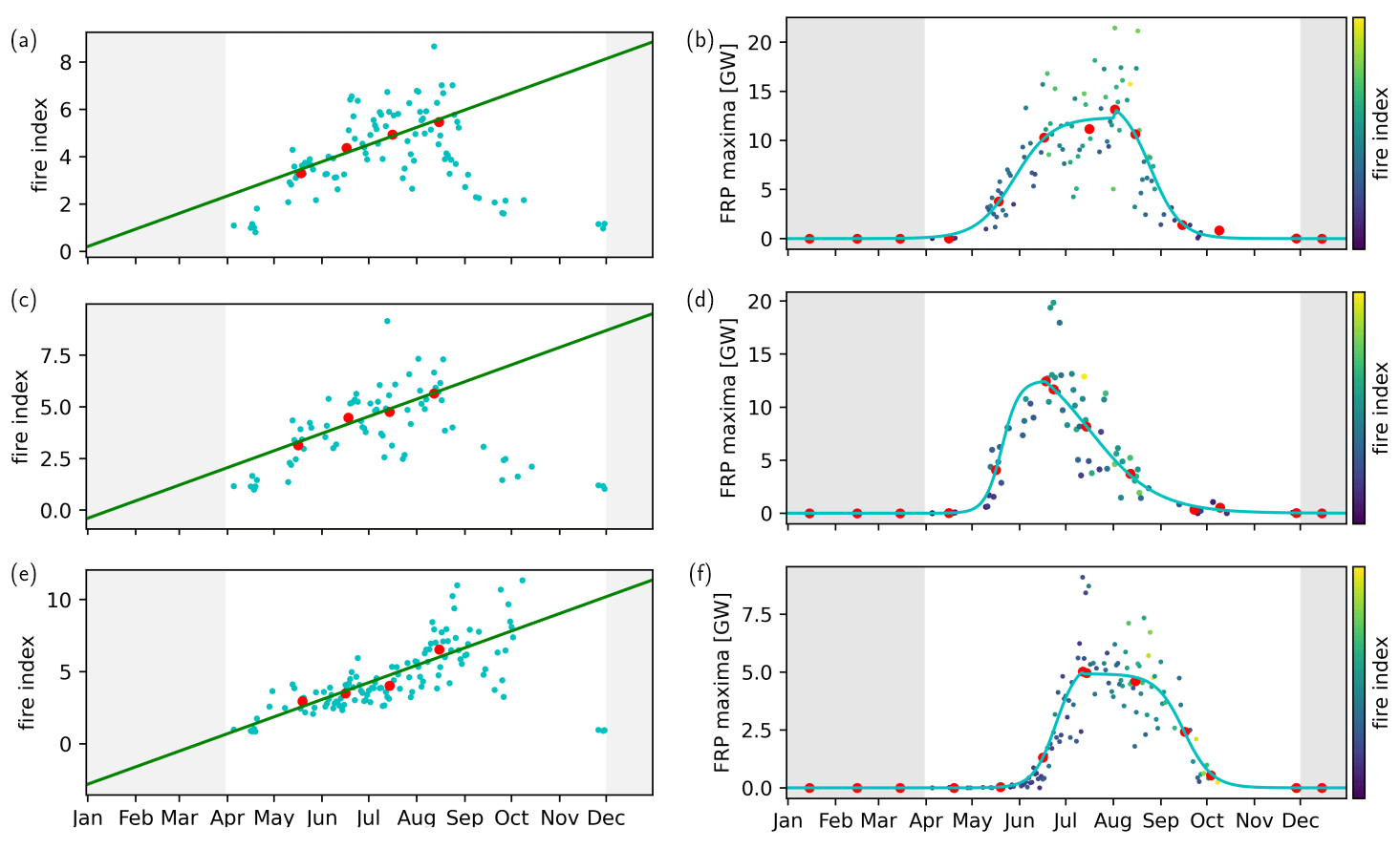
Figure 1 Training dataset. Fire index values and reference curves between April and November in 2010 for the areas located at 9.00^∘ S and 18.00^∘ E, 7.50^∘ S and 21.00^∘ E, and 13.50^∘ S and 16.50^∘ E from top to bottom row, respectively. The red dots denote monthly-mean values. A more detailed description of the figure is in the text.

The African savannah terrain was chosen as the test subject because the fires in it during the dry season come in great quantities on a daily basis. The chosen region is confined by the geographic coordinates [1.5, 19.5]^∘ S and [13.5, 33.0]^∘ E, which represent the centre points of 182 evenly spaced areas of size $\mathrm{1.5}{}^{\circ }\times \mathrm{1.5}{}^{\circ }$ (Fig. 4a). The dry season of the region is automatically included in the data used for the model fitting.

The model was parameterized using the data from 2010, and the model is applied and evaluated against the data for the fire season of 2018. The selection of distant years for training and evaluation demonstrates the stability of the method, as well as highlights the persistence of the regional fire ignition patterns, which did not change over almost a decade.

We present three examples of the model application for the three areas sized $\mathrm{1.5}{}^{\circ }\times \mathrm{1.5}{}^{\circ }$ located in northern Angola, the southern Democratic Republic of the Congo, and southern Angola, with the centre points at 9.00^∘ S and 18.00^∘ E, 7.50^∘ S and 21.00^∘ E, and 13.50^∘ S and 16.50^∘ E, respectively.

Figure 1 illustrates the parametrizations and prediction results of the areas. The left-hand panels show the fire index Eq. (4) values arising from the ERA5 meteorological data. The straight green line in the panels defines the weather-condition-dependent trend of the fire severity. It acts as the denominator of the meteorological component Eq. (2) fitted throughout monthly averages from May to August (red dots). The right-hand panels show the values for the FRP maxima observed by SEVIRI and (the colour bar) the value of the fire index. The blue line in the panels is the reference FRP curve W_r(n∣ϕ_r) of the area. It is also made to pass approximately through the monthly averages represented (red dots) apart from the maximum value. The maximum depicts an average of a few neighbouring values around the highest observed value in order to highlight the FRP maximum of the reference curve. Each point on the scatter plots of the panels in the figure represents a value of a cloudless or nearly cloudless day. The maximum cloud cover of each area is limited to 13.33 pixels per area of $\mathrm{0.5}{}^{\circ }\times \mathrm{0.5}{}^{\circ }$, i.e. of about 5 % tops. In order to simplify and speed up the calculation procedure, the cloud mask is checked only once at 13:30 LT (local time), which is more or less (within a window of plus or minus 2 h) the moment of the maximum daily FRP. The applicability of this simplification was tested more rigorously by checking the cloud mask every 15 min throughout the daylight hours. It did not have any significant effect on the selection of the cloudless or nearly cloudless days. The data used in the panels are for the year 2010. The values of the parameters corresponding to the curves in Fig. 1 are given in Table 1.

Table 1 Values for the parameter sets φ, ϕ_r, and ϕ_d given for three different areas employed in Eq. (1). The column names, areas 1–3, correspond, respectively, to their centre-point locations at 9.00^∘ S and 18.00^∘ E, 7.50^∘ S and 21.00^∘ E, and 13.50^∘ S and 16.50^∘ E.

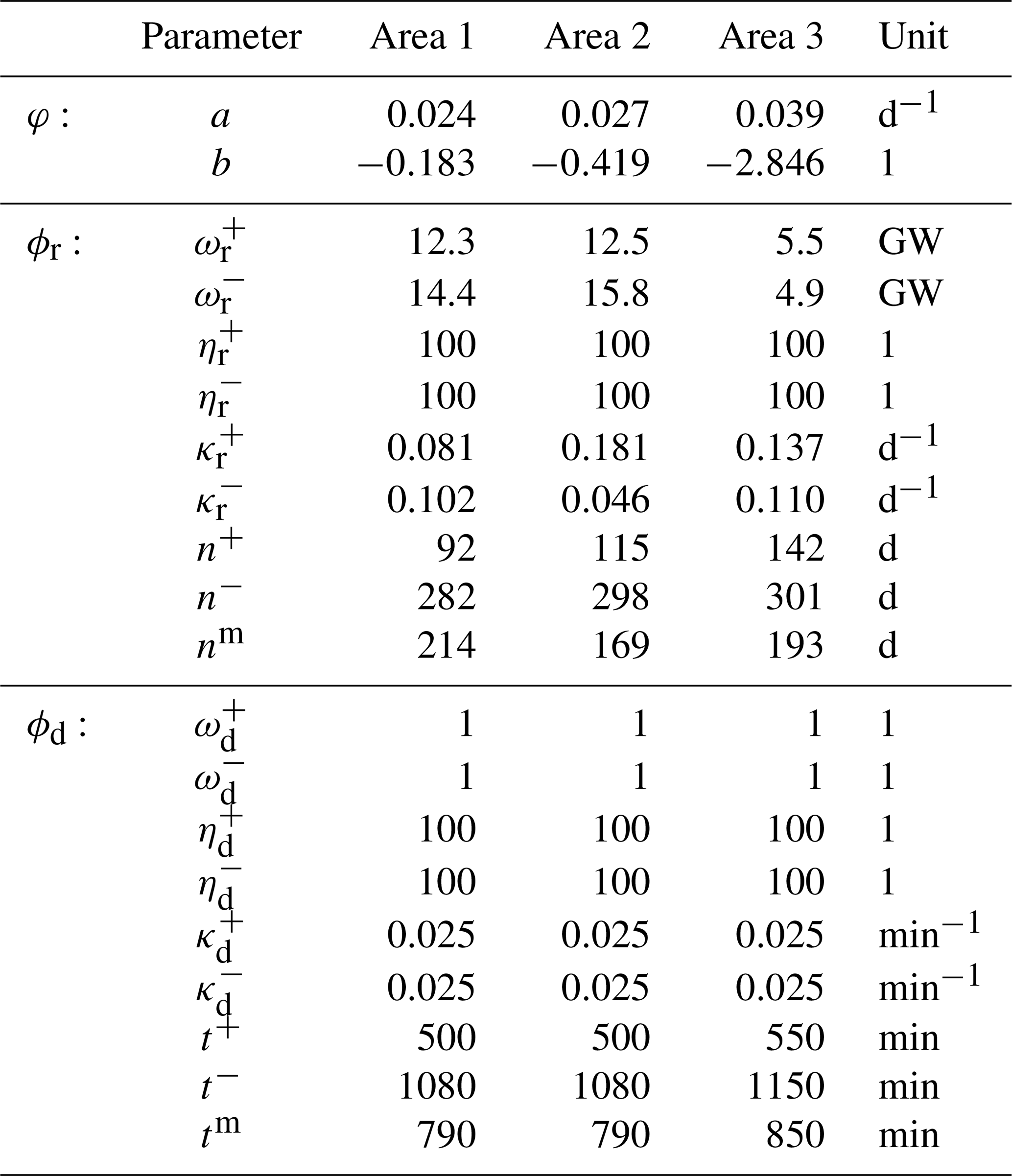
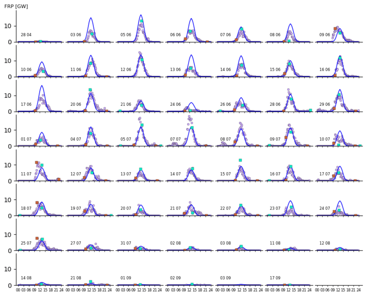
Figure 2 Test dataset. The solid dark blue lines are the predicted diurnal FRP curves, and the violet dots are the observed diurnal FRP of the area at 7.50^∘ S, 21.00^∘ E in 2018. The additional square points represent MODIS observations: the light blue ones are for Aqua and the brown ones for Terra. The horizontal axis is in the 24 h clock format and represents the local time at the centre point of the area. The date (day and month) is displayed on the left in each sub-figure.

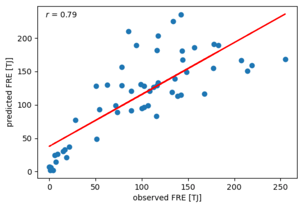
Figure 3 Predicted vs. observed diurnal FRE values (blue dots) arising from the predicted and SEVIRI-observed FRPs displayed in Fig. 2. The straight red line is the regression line $E_{\mathrm{pre}}=\mathrm{0.78}{E}_{\mathrm{obs}}+\mathrm{37.74}\mathrm{TJ}$.

Almost without exception, FRP of each area on each day can be (and is) characterized by a bell-shaped curve starting in the morning time, peaking somewhere around early afternoon, and ending in the early evening. The feature is seen in Fig. 2. These common characteristics may vary a little bit from area to area, as can be seen from $t^{\pm ,\mathrm{m}}$ values in Table 1. Figure 2 shows the predicted and observed diurnal FRP patterns for every cloudless (or nearly so) day within about 5 months of the dry season in 2018 for the area at 7.50^∘ S, 21.00^∘ E. The solid blue curves are the predictions given by Eq. (1) based on the parametrization made for 2010, and the violet dots are the SEVIRI observations for 2018. Note that the cloudless days are used only for evaluation purposes. When it comes to actual forecasting, it is irrelevant whether or not the day is cloudless as long as it is rainless. As can be seen in Fig. 2, in most cases, the correspondence between the predictions and observations is quite good, even though 8-year-old data were used for the parameterization. In the worst cases, the peak amplitudes differ from each other but in the majority of cases still stay within a factor of 2.

In order to assess the predictive power of the method, comparisons are made between observed and predicted daily FREs (given by the time integral of temporal FRP over the period of a day) over the course of the dry season. The diurnal FRP observations are integrated numerically by using Simpson's rule, and the predicted diurnal FRP predictions are calculated by an analytical integration. The accumulated energy within the time interval [t_i,t_f] is given by the temporal integral of Eq. (1), which can readily be written analytically by exploiting the result

$$\begin{array}{}\text{(6)}& \begin{array}{rl}& \underset{t_i}{\overset{t_f}{\int }}\mathrm{d}t{W}_{\mathrm{d}}\left(t\mid {\mathit{\varphi }}_{\mathrm{d}}\right)=\\ & \sum _{\mathit{ϵ}=\pm }{\displaystyle \frac{\mathit{ϵ}}{{\mathit{\kappa }}_{\mathrm{d}}^{\mathit{ϵ}}}}\mathrm{\Theta }\left(\mathit{ϵ}\left(t^{\mathrm{m}}-t\right)\right)\ln {\displaystyle \frac{{\mathit{\eta }}_{\mathrm{d}}^{\mathit{ϵ}}+\exp \left[\mathit{ϵ}{\mathit{\kappa }}_{\mathrm{d}}^{\mathit{ϵ}}(t-t^{\mathit{ϵ}})\right]}{{\mathit{\eta }}_{\mathrm{d}}^{\mathit{ϵ}}+\exp \left[\mathit{ϵ}{\mathit{\kappa }}_{\mathrm{d}}^{\mathit{ϵ}}\left(t^{\mathrm{m}}-t^{\mathit{ϵ}}\right)\right]}}{|}_{t_i}^{t_f}.\end{array}\end{array}$$

The definite integral in Eq. (6) has three different solutions depending on the values of the integration limits. In the results, the solution that arises from the integral that crosses both the ascending and descending sides of a bell-shaped curve is used every time.

Figure 4 Correlation map between observed and predicted FREs of areas whose dry season is between April and November. In the r values the zero before the decimal point is omitted. The shaded rectangle on the map of Africa in (a) encloses the geographic test region spanned by the geographic coordinates [1.5, 19.5]^∘ S and [13.5, 33.0]^∘ E. Panel (b) illustrates a magnification of the test region, which contains all the $\mathrm{1.5}{}^{\circ }\times \mathrm{1.5}{}^{\circ }$ sized and evenly distributed areas in which the sum of the observed FRE values of the days that are unmasked by clouds over the fire season exceeds 1 PJ.

The scatter plot of Fig. 3 illustrates the correlation between the observed and predicted FREs of Fig. 2. For example, the three areas denoted by 1–3 in Table 1 have the r values of 0.89, 0.79, and 0.75, respectively. The map of Fig. 4 sums up the respective FRE correlations of the areas which meet the conditions set out in the text. Note that FRE represents the diurnal energy of fires, which is a time-independent quantity and is therefore independent of how the corresponding FRP is located on the time axis. In most cases the r value exceeds 0.6, which indicates a moderate to very strong correlation between observations and predictions and that the method possesses some true predictive power. Areas where the observed total seasonal FRE in the prediction year 2018 is less than 1 PJ are omitted because of anticipated low and/or irregular fire intensity and thus low predictability. Out of the total of 182 areas, 106 are included areas concentrated in the centre of the region, and the other 76 are excluded ones located at the periphery of the fire-prone region. The ratio of the sums of observed and predicted fire seasonal FREs over all 106 areas depicted in Fig. 4b is 1.39; i.e. the model over-predicts the FRE by 39 %. Some part of the over-prediction may be justified. In many cases, the observed FRP values are relatively lower on Sundays than on any other day of the week, which presumably corresponds to the lower agriculture activity and, consequently, the ignition intensity during the weekends. Also, the smoke from fires may mask them, to some extent, and hence reduce the observed FRP. Finally, the smallest predicted fires may be below the SEVIRI detection limit.

A comparison with MODIS generally confirmed the conclusions. With the better spatial resolution and lower detection limit, MODIS FRPs were predominantly consistent with those of SEVIRI, as can be seen in Fig. 2. MODIS satellites Aqua and Terra overpass the area on a daily basis at the same time each day. Aqua typically observes the area around noon and midnight and Terra in the morning and evening. However, the periods of high fire intensity are quite narrow in the considered areas, which practically leaves only the mid-day Aqua overpass as the main source of information. For example, in Fig. 2, the time interval between two subsequent MODIS observations is considerably longer than the characteristic duration of the fire in the area. Such short fires would pose a general problem for low-orbit satellites also in other parts of the globe.

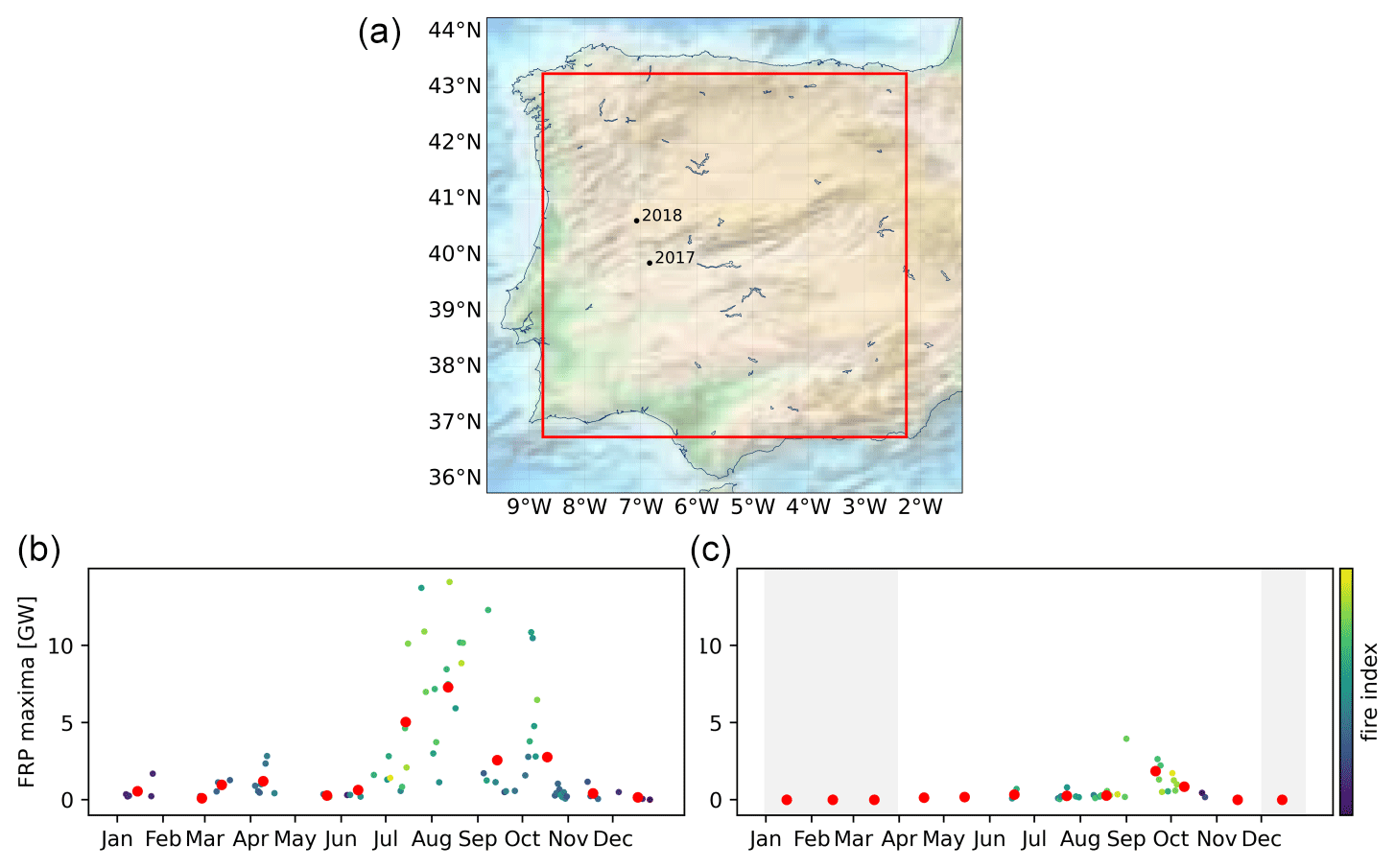
Figure 5 Panel (a) depicts an irregular fire test area enclosed by the red square which lies within the Iberian Peninsula. The area has a size of $\mathrm{6.5}{}^{\circ }\times \mathrm{6.5}{}^{\circ }$ with the centre point at 40.00^∘ N, 5.50^∘ W in Spain. Panel (b) shows FRP maxima of the area on cloud-free days for the year 2017 based on data over the full year. Panel (c) is the same as (b) but for the period of April to November 2018. The red dots denote monthly-mean FRP maxima. In panel (a) the average locations of the fires for both years are also marked.

4.2 Irregularly ignited fires in an area of the Iberian Peninsula

With irregularly ignited wildfires, such as forest fires and other wildfires started unintentionally or otherwise for no good reason, it is more difficult to make reasonable day-by-day predictions. That is because such fires exhibit low fire density, and even if the weather conditions for fires are favourable, they do not necessarily occur within a specified area. The problem of predicting the fire ignitions becomes dominant, unlike in the above-considered regions in Africa, where the fire ignition is a daily routine due to specific agricultural practices. For regions with irregular fires, wider spatial and longer temporal averaging might be needed to achieve some predictive power. On the downside, the reduction in spatio-temporal resolution reduces the quality of predictions, which may not be sufficient for reasonable-quality emission predictions. As an illustration of the arising difficulties, the current prediction model was parameterized and applied to forest fires considering almost the entire Iberian Peninsula as a single fire-prone area.

Figure 5 shows FRP maximum values of two subsequent years, 2017 and 2018, and their monthly averages emitted by nearly the whole Iberian Peninsula. The Forest Fire Danger Index (FFDI, Mark 5) (Noble et al., 1980) with the given drought factor accompanied by the Keetch–Byram drought index (KBDI) (Keetch and Byram, 1968), with the correction given in Alexander (1990), for the soil dryness is used as a reference for the incidence of wildfires in the area. The FFDI uses meteorological variables of air temperature, relative humidity, wind speed, and precipitation.

A comparison between the two panels of the figure shows the essence of the issue: the fires are not confined to a specific period of time but instead follow the complicated combination of short-term (days) and long-term (months) weather developments and human activities. The FFDI does not correlate well with the FRP strength between the 2 years, which is clearly seen especially around August when both years have several comparable values, with a wide range of values for 2017 and zeros for 2018. For such a fire pattern, the model developed above is too restrictive. One reason for this is that the method relies on the regular daily fire ignition, whereas forest fires are ignited sporadically. Another reason is that the forest fires do not exhibit as clear cycles throughout the years as the savannah fires in Africa. Moreover, extreme weather phenomena like powerful storms may further complicate the pattern. An example of this can be seen in Fig. 5a, in which the strong FRP peak in mid-October 2017 represents Iberian forest fires aggravated by high winds of tropical storm Ophelia as it passed by off the coast of Portugal. Especially on the 15th of October, on the day Ophelia hit the coast of Portugal the hardest, Iberia faced an exceptional firestorm. On that day, SEVIRI observed an FRP value exceeding 50 GW even though the area was heavily covered by clouds. This value is not displayed in the figure since it was not the true cloud-free observation.

The stochasticity of the fire occurrence (i.e. the number of fires or, alternatively, the amount of FRP) in an area can be decreased by extending the area and/or the time frame of the occurrence from instantaneous to longer. Nevertheless, forecasts should ideally predict the fire occurrence with the time dependence as done in this paper. Also, the area size should ideally be as small as possible. However, since the fire occurrence varies from area to area, the optimal area size into which a region should be evenly divided so that the areas remain sufficiently predictable depends on the chosen region. Due to the inherent stochasticity of the fire ignition, in the areas where the typical occurrence of fires is not exceptionally high the daily number of fires varies randomly even on consecutive days with the same weather conditions. This is the case, for example, with both in the excluded fringe areas of the region in Africa depicted in Fig. 4 and the area in Iberia depicted in Fig. 5. The more the weather favours wildfires, the greater the variation range is, but still nothing can be said with certainty about the daily fire occurrence and its temporal evolution. It is all about luck how many (if any) fires break out in the area on a day favourable to wildfires. This is in contrast to the case of African savannah fires, where these uncertainties are often within reasonable bounds due to regular ignitions. For example, as Fig. 1 illustrates, during the dry seasons, the African savannah fire occurrence (FRP) is always non-zero, much less arbitrary, and quite predictable. Moreover, as the Iberian case above indicates, in such conventional areas with low fire activity not only do daily occurrences vary widely but also annual ones. As an example within Fennoscandia, since the mid-1990s, the number of annual wildfires has ranged in Finland from approximately 1000 to 6000 and in Sweden from approximately 2500 to 8500 (Vanha-Majamaa et al., 2021), and in the Republic of Karelia between the years 1956 and 2019, the number of annual fires has ranged from 35 to 1872 (Lindberg et al., 2021) with values jumping up and down.

5 Summary

The presented phenomenological weather-dependent spatio-temporal fire prediction method showed promising results in predicting the wildfires in the African savannah environment under regular anthropogenic stress. The region showed stable fire ignition patterns over a long time, leaving the actual meteorological conditions as practically the only driving factor. As a result, the model parameterized with the 2010 fire and weather data was successfully applied for the 2018 fire season: the temporal correlation coefficient for a majority of predicted areas approached or exceeded 0.8–0.9. In more dynamically evolving regions, it may be advantageous to use the previous year's data for the parametrization.

It is possible that there are other fire-rich regions in the world other than the savannah of south-central Africa that can also be predicted fairly well. The method presented here is generally applicable to any region of the globe with a regular daily and annual occurrence of wildfires, which depending on the characteristics of the area and the size chosen is of the same order of magnitude as in the African savannahs. The widest predictable regions are the most productive of wildfire emissions, representing the leading contributions to global wildfire emissions, and should therefore be primarily located and included in air quality simulations to improve simulation accuracy. Therefore, a general sensible strategy for implementing fire predictions in simulations is primarily to consider such regions either by the method described in this paper, which is very straightforward, or by some other similarly highly predictive method. Thereafter, efforts can be made to increase the number and extent of predictable regions by refining the model used towards limits where predictability breaks down. Stochasticity determines the limit of predictability, which is a model-independent property, and the most accurate predictions can only be based on the most complete and detailed data possible.

The initial hypothesis that the higher incidence of fires in the area leads to more accurate predictions was qualitatively confirmed. The robustness of the model was increasing with the size of the area and the number of fires. Wider spatial averaging increased the amount and regularity of the fire information at the expense of lower spatial resolution of emissions. However, the problem with resolution might be slightly ameliorated by determining the sub-areas where the fires are repeatedly concentrated.

The approach significantly relies on regularity of the fire ignition events but showed quite low efficiency for irregularly ignited forest fires on the Iberian Peninsula despite the very wide spatial averaging. For that area, FRP still correlated with the weather and soil moisture conditions, but the ignition events did not.

The experience of the current model development and application highlighted the importance of accounting for the effects of both natural and anthropogenic drivers of fires. The developed simple model, being sufficient for regions with regular anthropogenic fire ignitions, has no easy application in areas with irregular ignitions. More generally, due to the inherently random nature of the initial ignition of wildfires, the development of universal fire prediction models with sensible temporal and spatial resolution remains a difficult if not unachievable challenge.