the Creative Commons Attribution 4.0 License.
the Creative Commons Attribution 4.0 License.
 | 26 Feb 2021
Multilayer-HySEA model validation for landslide-generated tsunamis – Part 2: Granular slides
Cipriano Escalante
Manuel J. Castro
The final aim of the present work is to propose a NTHMP-benchmarked numerical tool for landslide-generated tsunami hazard assessment. To achieve this, the novel Multilayer-HySEA model is validated using laboratory experiment data for landslide-generated tsunamis. In particular, this second part of the work deals with granular slides, while the first part, in a companion paper, considers rigid slides. The experimental data used have been proposed by the US National Tsunami Hazard and Mitigation Program (NTHMP) and were established for the NTHMP Landslide Benchmark Workshop, held in January 2017 at Galveston (Texas). Three of the seven benchmark problems proposed in that workshop dealt with tsunamis generated by rigid slides and are collected in the companion paper (Macías et al., 2021). Another three benchmarks considered tsunamis generated by granular slides. They are the subject of the present study. The seventh benchmark problem proposed the field case of Port Valdez, Alaska, 1964 and can be found in Macías et al. (2017). In order to reproduce the laboratory experiments dealing with granular slides, two models need to be coupled: one for the granular slide and a second one for the water dynamics. The coupled model used consists of a new and efficient hybrid finite-volume–finite-difference implementation on GPU architectures of a non-hydrostatic multilayer model coupled with a Savage–Hutter model. To introduce the multilayer model more fluidly, we first present the equations of the one-layer model, Landslide-HySEA, with both strong and weak couplings between the fluid layer and the granular slide. Then, a brief description of the multilayer model equations and the numerical scheme used is included. The dispersive properties of the multilayer model can be found in the companion paper. Then, results for the three NTHMP benchmark problems dealing with tsunamis generated by granular slides are presented with a description of each benchmark problem.
- Article
(3096 KB) - Full-text XML
- Companion paper
- BibTeX
- EndNote


Following the introduction of the companion paper Macías et al. (2021), a landslide tsunami model benchmarking and validation workshop was held on 9–11 January 2017 in Galveston, TX. This workshop was organized on behalf of the NOAA National Weather Service's National Tsunami Hazard Mitigation Program (NTHMP) Mapping and Modeling Subcommittee (MMS) with the expected outcome being to (i) develop a set of community-accepted benchmark tests for validating models used for landslide tsunami generation and propagation in NTHMP inundation mapping work; (ii) develop workshop documentation and a web-based repository, for benchmark data, model results, and workshop documentation, results, and conclusions; and (iii) provide recommendations as a basis for developing best-practice guidelines for landslide tsunami modeling in NTHMP work.
A set of seven benchmark tests was selected (Kirby et al., 2018). The selected benchmarks were taken from a subset of available laboratory data sets for solid slide experiments (three of them) and deformable slide experiments (another three) that included both submarine and subaerial slides. Finally, a benchmark based on a historic field event (Valdez, AK, 1964) closed the list of proposed benchmarks. The EDANYA group (https://www.uma.es/edanya, last access: 21 February 2021) from the University of Malaga participated in the aforementioned workshop, and the numerical codes Multilayer-HySEA and Landslide-HySEA were used to produce our modeled results. We presented numerical results for six out of the seven benchmark problems proposed, including the field case (Macías et al., 2017). The sole benchmark we did not perform at the time was BP6, for which numerical results are included here.
The present work aims at showing the numerical results obtained with the Multilayer-HySEA model in the framework of the validation effort described above for the case of granular-slide-generated tsunamis for the complete set of the three benchmark problems proposed by the NTHMP. However, the ultimate goal of the present work is to provide the tsunami community with a numerical tool, tested and validated meeting the defined criteria for the NTHMP, for landslide-generated tsunami hazard assessment. This NTHMP acceptance has already been achieved by the Tsunami-HySEA model for the case of earthquake-generated tsunamis (Macías et al., 2017, 2020a, c).
Fifteen years ago, at the beginning of the century, solid block landslide modeling challenged researchers and was undertaken by a number of authors (see companion paper, Macías et al., 2021, for references), and laboratory experiments were developed for those cases and for tsunami model benchmarking. In contrast, some early models (e.g., Heinrich, 1992; Harbitz et al., 1993; Rzadkiewicz et al., 1997; Fine et al., 1998) and a number of more recent models have simulated tsunami generation by deformable slides, based either on depth-integrated two-layer model equations or on solving more complete sets of equations in terms of featured physics (dispersive, non-hydrostatic, Navier–Stokes). Examples include solutions of 2D or 3D Navier–Stokes equations to simulate subaerial or submarine slides modeled as dense Newtonian or non-Newtonian fluids (Ataie-Ashtiani and Shobeyri, 2008; Weiss et al., 2009; Abadie et al., 2010, 2012; Horrillo et al., 2013), flows induced by sediment concentration (Ma et al., 2013), or fluid or granular flow layers penetrating or failing underneath a 3D water domain – for example, the two-layer models of Macías et al. (2015) or González-Vida et al. (2019), where a fully coupled non-hydrostatic SW/Savage–Hutter model is used, or the model used in Ma et al. (2015) and Kirby et al. (2016), in which the upper water layer is modeled with the non-hydrostatic σ-coordinate 3D model NHWAVE (Ma et al., 2012). For a more comprehensive review of recent modeling work, see Yavari-Ramshe and Ataie-Ashtiani (2016). A number of recent laboratory experiments have modeled tsunamis generated by subaerial landslides composed of gravel (Fritz et al., 2004; Ataie-Ashtiani and Najafi-Jilani, 2008; Heller and Hager, 2010; and Mohammed and Fritz, 2012) or glass beads (Viroulet et al., 2014). For deforming underwater landslides and related tsunami generation, 2D experiments were performed by Rzadkiewicz et al. (1997), who used sand, and Ataie-Ashtiani and Najafi-Jilani (2008), who used granular material. Well-controlled 2D glass bead experiments were reported and modeled by Grilli et al. (2017) using the model of Kirby et al. (2016).
The benchmark problems performed in the present work are based on the laboratory experiments of Kimmoun and Dupont (see Grilli et al., 2017) for BP4, Viroulet et al. (2014) for BP5, and Mohammed and Fritz (2012) for BP6. The basic reference for these three benchmarks, but also the three related to solid slides and the Alaska field case, all of them proposed by the NTHMP, is Kirby et al. (2018). That is a key reference for readers interested in the benchmarking initiative which the present work is based on.
First we consider the Landslide-HySEA model, applied in Macías et al. (2015) and González-Vida et al. (2019), which for the case of one-dimensional domains reads
where g is the gravity acceleration (g=9.81 m s−2); H(x) is the non-erodible (does not evolve in time) bathymetry measured from a given reference level; zs(x, t) represents the thickness of the layer of granular material at each point x at time t; h(x, t) is the total water depth; η(x, t) denotes the free surface (measured form the same fixed reference level used for the bathymetry, for example, the mean sea surface) and is given by ; u(x, t) and us(x, t) are the averaged horizontal velocity for the water and for the granular material, respectively; and is the ratio of densities between the ambient fluid and the granular material. The term na(us−u) parameterizes the friction between the fluid and the granular layer. Finally, the term τP(x, t) represents the friction between the granular slide and the non-erodible bottom surface. It is parameterized as in Pouliquen and Forterre (2002), and it is described in the next section.
System Eq. (1) presents the difficulty of considering the complete coupling between sediment and water, including the corresponding coupled pressure terms. That makes its numerical approximation more complex. Moreover, it also makes it difficult to consider its natural extension to non-hydrostatic flows.
Now, if ∂xη is neglected in the momentum equation of the granular material, that is, the fluctuation of pressure due to the variations of the free surface is neglected in the momentum equation of the granular material, then the following weakly coupled system could be obtained:
where the first system is the standard one-layer shallow-water system and the second one is the one-layer reduced-gravity Savage–Hutter model (Savage and Hutter, 1989) that takes into account that the granular landslide is underwater. Note that the previous system could be also adapted to simulate subaerial/submarine landslides by a suitable treatment of the variation of the gravity terms. Under this formulation, it is now straightforward to improve the numerical model for the fluid phase by including non-hydrostatic effects.
In the present study, the governing equations of the landslide motion are derived in Cartesian coordinates. In some cases where steep slopes are involved, landslide models based on local coordinates allow representing the slide motion better. However, when general topographies are considered and not only simple geometries, landslide models based on local coordinates also introduce some difficulties on the final numerical model and on its implementation compromising, at the same time, the computational efficiency of the numerical model. Here, we focus on the hydrodynamic component of the system, and that is one of the reasons for choosing a simple landslide model based on Cartesian coordinates. Of course, the strategies presented here can also be adapted for more sophisticated landslide models. For example, in Garres-Díaz et al. (2021) a non-hydrostatic model for the hydrodynamic part that is similar to the one presented here for the case of a single layer was introduced. In the work mentioned above, the authors study the influence of coupling the hydrodynamic model with a granular model that is derived in both reference systems: Cartesian and local coordinates. The front positions calculated with the Cartesian model progress faster, and, after some time, they are slightly ahead compared with the local coordinate model solution (see, for instance, Fig. 4 in Garres-Díaz et al., 2021). This is due to the fact that the Cartesian model uses the horizontal velocity instead of the velocity tangent to the topography. In any case, the differences between the two models are not very noticeable. A granular slide model based on local coordinates might give better results. However, when introducing a non-hydrostatic pressure, the model is closer to a 3D solver. In such a case, the influence on the reference coordinate system barely exists. That is the reason why in Garres-Díaz et al. (2021) both non-hydrostatic models based on different coordinate systems show similar results. In any case, although on the present work we focus on the hydrodynamic part, it can be observed on the benchmark tests that the numerical results are in very good agreement with the laboratory-measured data, despite the simple landslide model chosen here.
The Multilayer-HySEA model implements a two-phase model intended to reproduce the interaction between the slide granular material (submarine or subaerial) and the fluid. In the present work, a multilayer non-hydrostatic shallow-water model is considered for modeling the evolution of the ambient water (see Fernández-Nieto et al., 2018), and for simulating the kinematics of the submarine/subaerial landslide the Savage–Hutter model (Eq. 3) is used. The coupling between these two models is performed through the boundary conditions at their interface. The parameter r represents the ratio of densities between the ambient fluid and the granular material (slide liquefaction parameter). Usually
where ρs stands for the typical density of the granular material, ρf is the density of the fluid (ρs>ρf), both constant, and φ represents the porosity (). In the current work, the porosity, φ, is supposed to be constant in space and time, and, therefore, the ratio r is also constant. This ratio ranges from 0 to 1 (i.e., ) and, even on a uniform material, is difficult to estimate as it depends on the porosity (and ρf and ρs are also supposed to be constant). Typical values for r are in the interval [0.3, 0.8].

The fluid model
The ambient fluid is modeled by a multilayer non-hydrostatic shallow-water system (Fernández-Nieto et al., 2018) to account for dispersive water waves. The model considered, that is obtained by a process of depth-averaging of the Euler equations, can be interpreted as a semi-discretization with respect to the vertical coordinate. In order to take into account dispersive effects, the total pressure is decomposed into the sum of hydrostatic and non-hydrostatic components. In this process, the horizontal and vertical velocities are supposed to have constant vertical profiles. The resulting multilayer model admits an exact energy balance, and when the number of layers increases, the linear dispersion relation of the linear model converges to that of Airy's theory. Finally, the model proposed in Fernández-Nieto et al. (2018) can be written in compact form as
for α∈{1, 2, …, L}, with L the number of layers and where the following notation has been used:
where f denotes one of the generic variables of the system, i.e., u, w, and p; and, finally,
Figure 1 shows a schematic picture of the model configuration, where the total water height h is decomposed along the vertical axis into L≥1 layers. The depth-averaged velocities in the x and z directions are written as uα and wα, respectively. The non-hydrostatic pressure at the interface is denoted by . The free-surface elevation measured from a fixed reference level (for example the still-water level) is written as η and , where again H(x) is the unchanged non-erodible bathymetry measured from the same fixed reference level. τα=0 for α>1, and τ1 is given by
where τb stands for an classical Manning-type parameterization for the bottom shear stress and, in our case, is given by
and na(us−u1) accounts for the friction between the fluid and the granular layer. The latest two terms are only present at the lowest layer (α=1). Finally, for α=1, …, L−1, parameterizes the mass transfer across interfaces, and those terms are defined by
Here we suppose that ; this means that there is no mass transfer through the sea floor or the water free surface. In order to close the system, the boundary condition
is imposed at the free-surface and the boundary conditions
are imposed at the bottom. The last two conditions enter into the incompressibility relation for the lowest layer (α=1), given by
It should be noted that both models, the hydrodynamic model described here and the morphodynamic model described in the next subsection, are coupled through the unknown zs, which, in the case of the model described here, is present in the equations and in the boundary condition ().
Some dispersive properties of system Eq. (5) were originally studied in Fernández-Nieto et al. (2018). Moreover, for a better-detailed study on the dispersion relation (such as phase velocity, group velocity, and linear shoaling) the reader is referred to the companion paper Macías et al. (2021).
Along the derivation of the hydrodynamic model presented here, the rigid-lid assumption for the free surface of the ambient fluid is adopted. This means that pressure variations induced by the fluctuation on the free surface of the ambient fluid over the landslide are neglected.
The landslide model
The 1D Savage–Hutter model used and implemented in the present work is given by system Eq. (3). The friction law τP (Pouliquen and Forterre, 2002) is given by the expression
where μ is a constant friction coefficient with a key role, as it controls the movement of the landslide. Usually μ is given by the Coulomb friction law as the simpler parameterization that can be used in landslide models. However, it is well known that a constant friction coefficient does not allow us to reproduce steady uniform flows over rough beds observed in the laboratory for a range of inclination angles. To reproduce these flows, in Pouliquen and Forterre (2002), the authors introduce an empirical friction coefficient μ that depends on the norm of the mean velocity us, on the thickness zs of the granular layer, and on the Froude number . The friction law is given by
with
where ds represents the mean size of grains. β=0.136 and are empirical parameters. tan (δ1) and tan (δ2) are the characteristic angles of the material, and tan (δ3) is other friction angle related to the behavior when starting from rest. This law has been widely used in the literature (see, e.g., Brunet et al., 2017).
Note that the slide model can also be adapted to simulate subaerial landslides. The presence of the term (1−r) in the definition of the Pouliquen–Forterre friction law is due to the buoyancy effects, which must be taken into account only in the case that the granular material layer is submerged in the fluid. Otherwise, this term must be replaced by 1.
System Eq. (3) can be written in the following compact form:
being
Analogously, the multilayer non-hydrostatic shallow-water system Eq. (5) can also be expressed in a similar way:
where
and Bf(Uf)∂x(Uf) contains the non-conservative products involving the momentum transfer across the interfaces, and, finally, Sf(Uf) represents the friction terms,
The non-hydrostatic corrections in the momentum equations are given by
and, finally, the operator related with the incompressibility condition at each layer is given by
The discretization of systems (Eqs. 6 and 7) becomes difficult. In the present work, the natural extension of the numerical schemes proposed in Escalante et al. (2018a, b) is considered. These authors propose, describe, and use a splitting technique. Initially, the systems (Eqs. 6 and 7) are expressed as the following non-conservative hyperbolic system:
Both equations are solved simultaneously using a second-order HLL (Harten–Lax–van Leer), positivity-preserving, and well-balanced, path-conservative finite-volume scheme (see Castro and Fernández-Nieto, 2012) and using the same time step. The synchronization of time steps is performed by taking into account the Courant–Friedrichs–Lewy (CFL) condition of the complete system Eq. (8). A first-order estimation of the maximum of the wave speed for system Eq. (8) is the following:
Then, the non-hydrostatic pressure corrections , ⋯, at the vertical interfaces are computed from
which requires the discretization of an elliptic operator that is done using standard second-order central finite differences. This results in a linear system than in our case is solved using an iterative scheduled Jacobi method (see Adsuara et al., 2016). Finally, the computed non-hydrostatic corrections are used to update the horizontal and vertical momentum equations at each layer, and, at the same time, the frictions Ss(Us) and Sf(Uf) are also discretized (see Escalante et al., 2018a, b). For the discretization of the Coulomb friction term, we refer the reader to Fernández-Nieto et al. (2008).
The resulting numerical scheme is well balanced for the water-at-rest stationary solution and is linearly L∞ stable under the usual CFL condition related to the hydrostatic system. It is also worth mentioning that the numerical scheme is positive preserving and can deal with emerging topographies. Finally, its extension to 2D is straightforward. For dealing with numerical experiments in 2D regions, the computational domain must be decomposed into subsets with a simple geometry, called cells or finite volumes. The 2D numerical algorithm for the hydrodynamic hyperbolic component of the coupled system is well suited to be parallelized and implemented in GPU architectures, as is shown in Castro et al. (2011). Nevertheless, a standard treatment of the elliptic part of the system does not allow the parallelization of the algorithms. The method used here and proposed in Escalante et al. (2018a, b) makes it possible that the second step can also be implemented on GPUs, due to the compactness of the numerical stencil and the easy and massive parallelization of the Jacobi method The above-mentioned parallel GPU and multi-GPU implementation of the complete algorithm results in much shorter computational times.
This section presents the numerical results obtained with the Multilayer-HySEA model for the three benchmark problems dealing with granular slides and the comparison with the measured lab data for the generated water waves. In particular, BP4 deals with a 2D submarine granular slide, BP5 with a 2D subaerial slide, and BP6 with a 3D subaerial slide. The description of all these benchmarks can be found in LTMBW (2017) and Kirby et al. (2018). In this paper, all units, unless otherwise indicated, will be expressed in the SI (International System of Units) units.
The model parameters required in each simulation are
The parameters g, r, nm, and ds are related to physical settings given in each experiment. β and γ are empirical parameters that were chosen as in the seminal paper of Pouliquen and Forterre (2002).
The friction angles δ1 and δ2 are characteristic angles of the material, and δ3 is related to the behavior of the slide motion when starting from the rest. Thus, the values of these angles strongly depend on the granular material. They were adjusted within a range of feasible values according to the references (Brunet et al., 2017; Mangeney et al., 2007; Pouliquen and Forterre, 2002):
In the present paper we have used the values
for the three benchmark problems, which is consistent with the values found in the literature. As noted in Mangeney et al. (2007), in general for real problems involving complex rheologies, smaller values of these parameters δi should be employed.
With regard to the sensitivity of the model to parameter variation, an appropriate sensitivity analysis can be performed, as is done in González-Vida et al. (2019). However, the aim of the present work was to prove if the non-hydrostatic model coupled with the granular model was able to accurately reproduce the three benchmarks considered.
Regarding the parameter denoting the buoyancy effect, for field cases, r=0.5 is usually taken, and then the parameter is eventually adjusted based on available field data. In general, the complexity of the rheology introduces a difficulty that is always present on the modeling as well as on the adjustment of the parameters. Moreover, the more sophisticated the model is (considering, for example, the rheology of the material), more input data will be required.
We would like to stress the simplicity of the slide model used here as a great advantage regarding parameter setup. Although the end user has to adjust some input parameters of the model, within a range of acceptable value, the simplicity of the proposed numerical model makes this task remain simple – not representing an obstacle to run the model. On the other hand, the efficient GPU implementation of the model allows for performing uncertainty quantification (see Sánchez-Linares et al., 2016) on a few parameters and investigating the sensitivity to them, varying on small ranges (as in González-Vida et al., 2019). This will be the aim of future works. When field or experimental observations are available, a different approach is proposed in Ferreiro-Ferreiro et al. (2020), where an automatic data assimilation strategy for a similar landslide non-hydrostatic model is proposed. The same strategy can be adapted for the model used here.
5.1 Benchmark problem 4: two-dimensional submarine granular slide
The first proposed benchmark problem for granular slides, BP4 in the list, aims to reproduce the generation of tsunamis by submarine granular slides modeled in the laboratory experiment by means of glass beads. The corresponding 2D laboratory experiments were performed at the École Centrale de Marseille (see Grilli et al., 2017, for a description of the experiment). A set of 58 (29 with their corresponding replicate) experiments were performed at the IRPHE (Institut de Recherche sur les Phénomènes Hors Equilibre) precision tank. The experiments were performed using a triangular submarine cavity filled with glass beads that were released by lifting a sluice gate and then moving down a plane slope, all underwater. Figure 2 shows a schematic picture of the experiment setup.
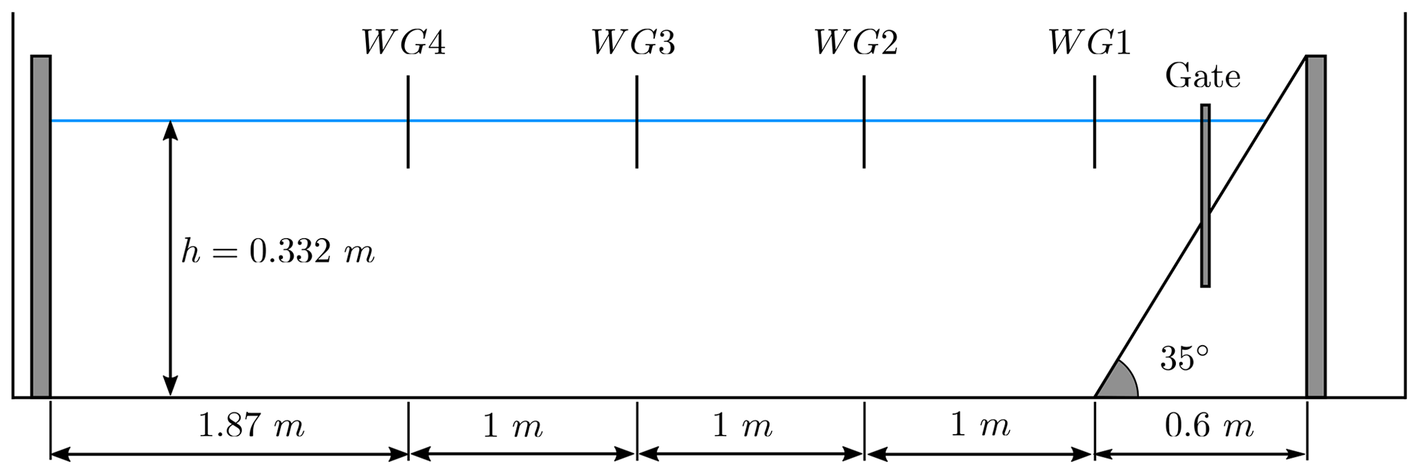
Figure 2BP4 sketch showing the longitudinal cross section of the IRPHE's precision tank. The figure shows the location of the plane slope, the sluice gate, and the four gages (WG1–WG4).
The one-dimensional domain [0, 6] is discretized with Δx=0.005 m, and wall boundary conditions are imposed. The simulated time is 10 s. The CFL number was set to 0.5, and model parameters take the following values:
Figure 3 depicts the modeled times series for the water height at the four wave gages and compares them with the lab-measured data. Note that the computed free surface matches well with the laboratory data for gauges WG2–WG4, both in amplitude and frequency. For gauge WG1, some mismatch is observed in amplitude, which could be explained by the simplicity of the landslide model and the absence of turbulent effects in the model.
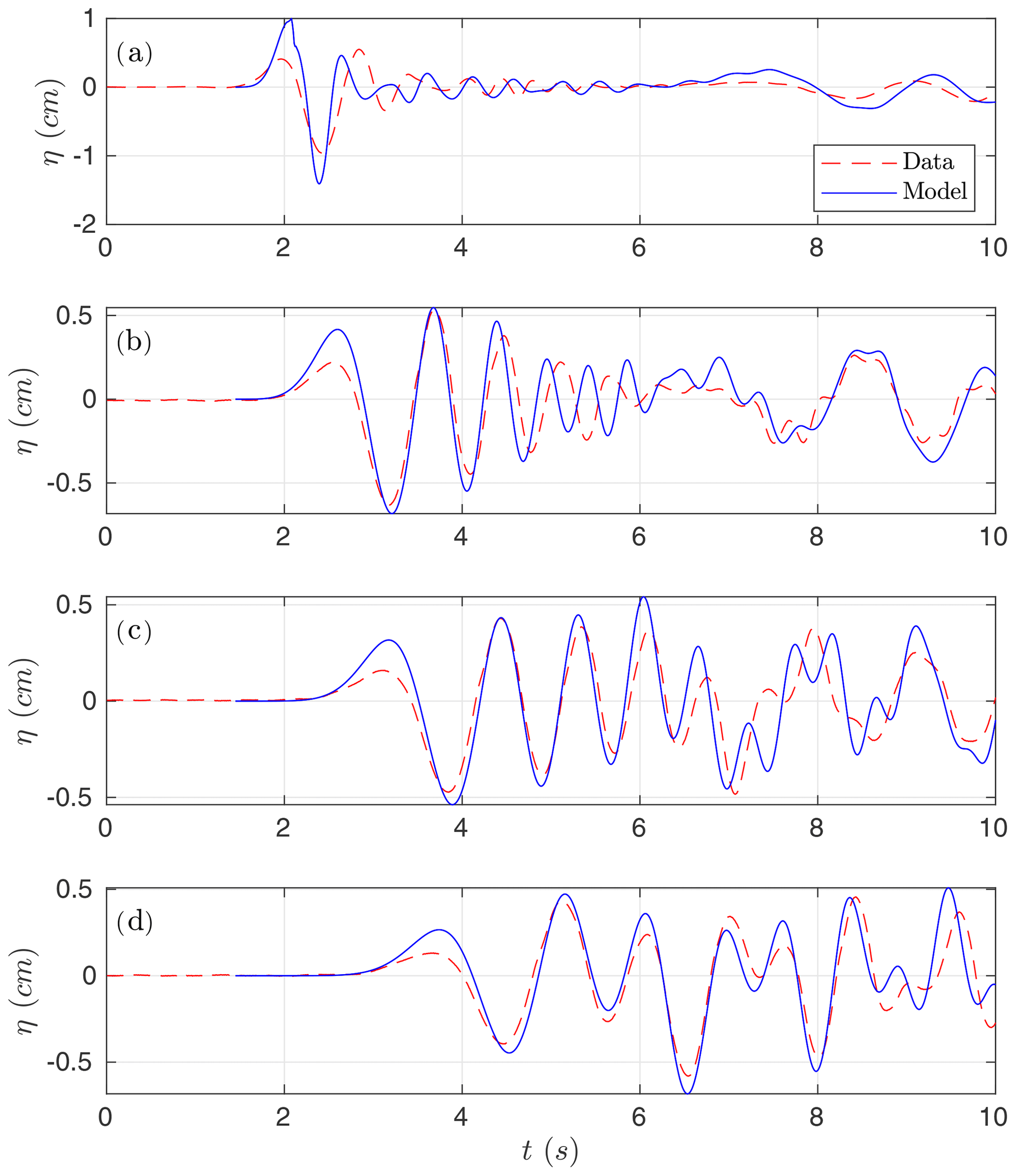
Figure 3Numerical time series for the simulated water surface (in blue) compared with lab-measured data (red) at wave gauges (a) WG1, (b) WG2, (c) WG3, and (d) WG4.
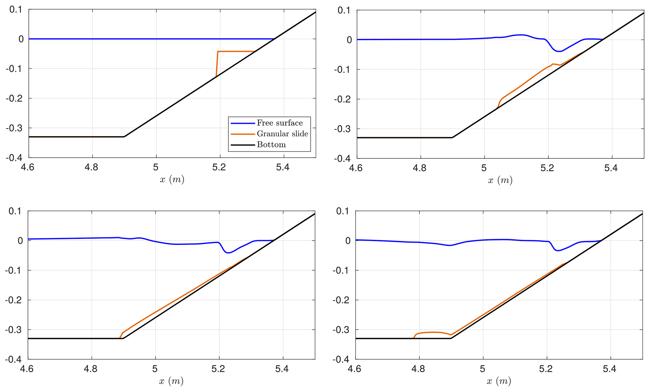
Figure 4Modeled location of the granular material and water free surface elevation at times t=0, 0.3, 0.6, and 0.9 s.
Figure 4 shows the location and evolution of the granular material and water free surface at several times during the numerical simulation. In Grilli et al. (2017) some snapshots of the landslide evolution are shown at different time steps. Compared to those snapshots, it can be observed that the location of the landslide front is well captured by the model, but there is some mismatch in the landslide shape at the front, mainly due to the simplicity of the landslide model considered here. In particular, we consider that density remains constant in the landslide layer during the simulation, which is not true due to the water entrainment.
In the numerical experiments presented in this section, the number of layers was set up to five. Similar results were obtained with a lower number of layers (four or three) but slightly closer to measured data when considering five layers. This justifies our choice in the present test problem. A larger number of layers does not further improve the numerical results. This may indicate that to get better numerical results, it is no longer a question related to the dispersive properties of the model (which improve with the number of layers) but is more likely due to some missing physics.
5.2 Benchmark problem 5: two-dimensional subaerial granular slide
This benchmark is based on a series of 2D laboratory experiments performed by Viroulet et al. (2014) in a small tank at the École Centrale de Marseille, France. The simplified picture of the setup for these experiments can be found in Fig. 5.
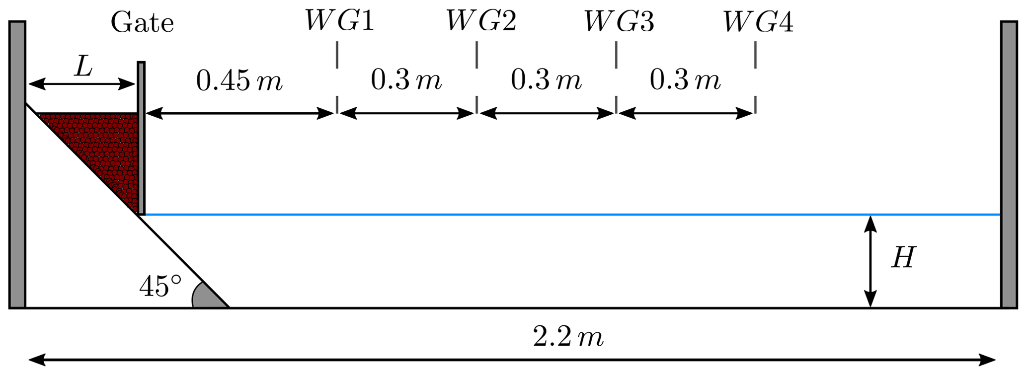
The granular material was confined in triangular subaerial cavities and composed of dry glass beads of diameter ds (which was varied) and density ρs=2500 km m−3. This was located on a plane with a 45∘ slope just on top of the water surface. Then the slide was released by lifting a sluice gate and coming in contact with water right away. The experimental setup used by Viroulet et al. (2014) consisted of a wave tank 2.2 m long, 0.4 m high, and 0.2 m wide.
The granular material is initially retained by a vertical gate on the dry slope. The gate is suddenly lowered, and in the numerical experiments, it should be assumed that the gate release velocity is large enough to neglect the time it takes the gate to withdraw. The front face of the granular slide touches the water surface at t=0. The initial slide shape has a triangular cross section over the width of the tank, with down-tank length L and front face height B=L as the slope angle is 45∘.
For the present benchmark, two cases are considered. Case 1 is defined by the following setup: ds=1.5 mm, H=14.8 cm, and L=11 cm. Case 2 is given by ds=10 mm, H=15 cm, and L=13.5 cm. The benchmark problem proposed consists of simulating the free-surface elevation evolution at the four gauges WG1 to WG4, where measured data are provided, for the two test cases described above.
The same model configuration as in the previous benchmark problem is used here. The vertical structure is reproduced using three layers in the present case. The one-dimensional domain is given by the interval [0, 2.2], and it is discretized using a step Δx=0.003 m. As boundary conditions, rigid walls were imposed. The simulation time is 2.5 s. The CFL number is set to 0.9, and the model parameters take the following values:
Finally ds was set to and depending on the test case.
Figure 6 shows the comparison for Case 1. In this case, the numerical results show a very good agreement when compared with lab-measured data, and, in particular, the two leading waves are very well captured. Figure 7 shows the comparison for Case 2. In this case, the agreement is good, but larger differences between model and lab measurements can be observed.
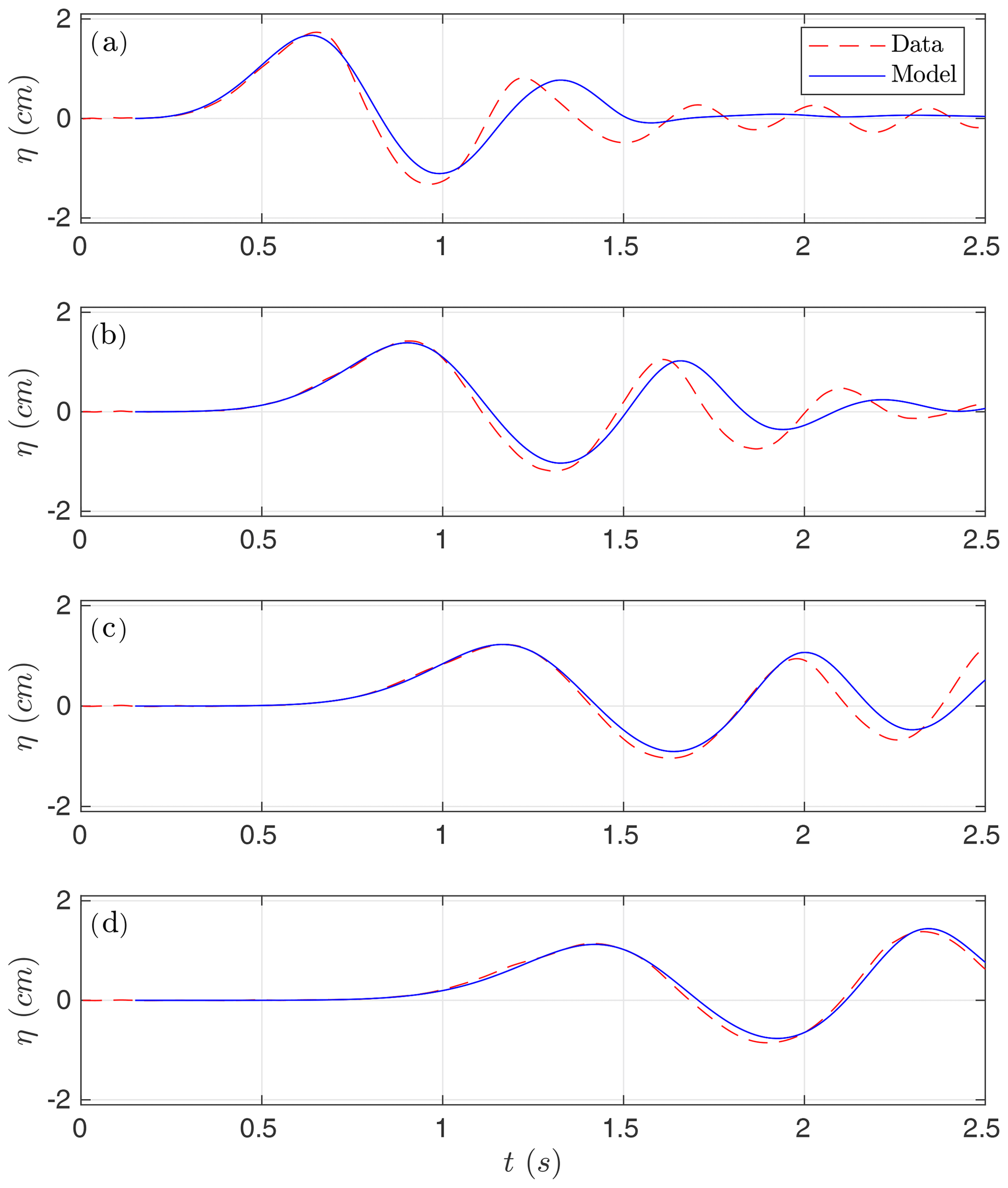
Figure 6Numerical time series for the simulated water surface (in blue) compared with lab-measured data (red). Case 1 at gauges (a) G1, (b) G2, (c) G3, and (d) G4.

Figure 7Numerical time series for the simulated water surface (in blue) compared with lab-measured data (red). Case 2 at gauges (a) G1, (b) G2, (c) G3, and (d) G4.
Two things can be concluded from the observation of Figs. 6 and 7: (1) a much better agreement is obtained for Case 1 than for Case 2 and (2) the agreement is better for gauges located farther from the slide compared with closer to the slide gauges. Although paradoxical, this second differential behavior among gauges can be explained as a consequence of the hydrodynamic component being much better resolved and simulated than the morphodynamic component (the movement of the slide material), which is obviously much more difficult to reproduce. But, at the same time, this implies a correct transfer of energy at the initial stages of the interaction between the slide and fluid.
Finally, Fig. 8 shows the location of the granular material and the free-surface elevation at several times for the numerical simulation of Case 1. In Viroulet et al. (2014) some snapshots of the landslide evolution are shown at different time steps that can be compared with Fig. 8. As for the benchmark problem 4, it can be seen that the location of the landslide front is well captured, but there is some mismatch in the landslide shape at the front, mainly due to the simplicity of the landslide model considered here.
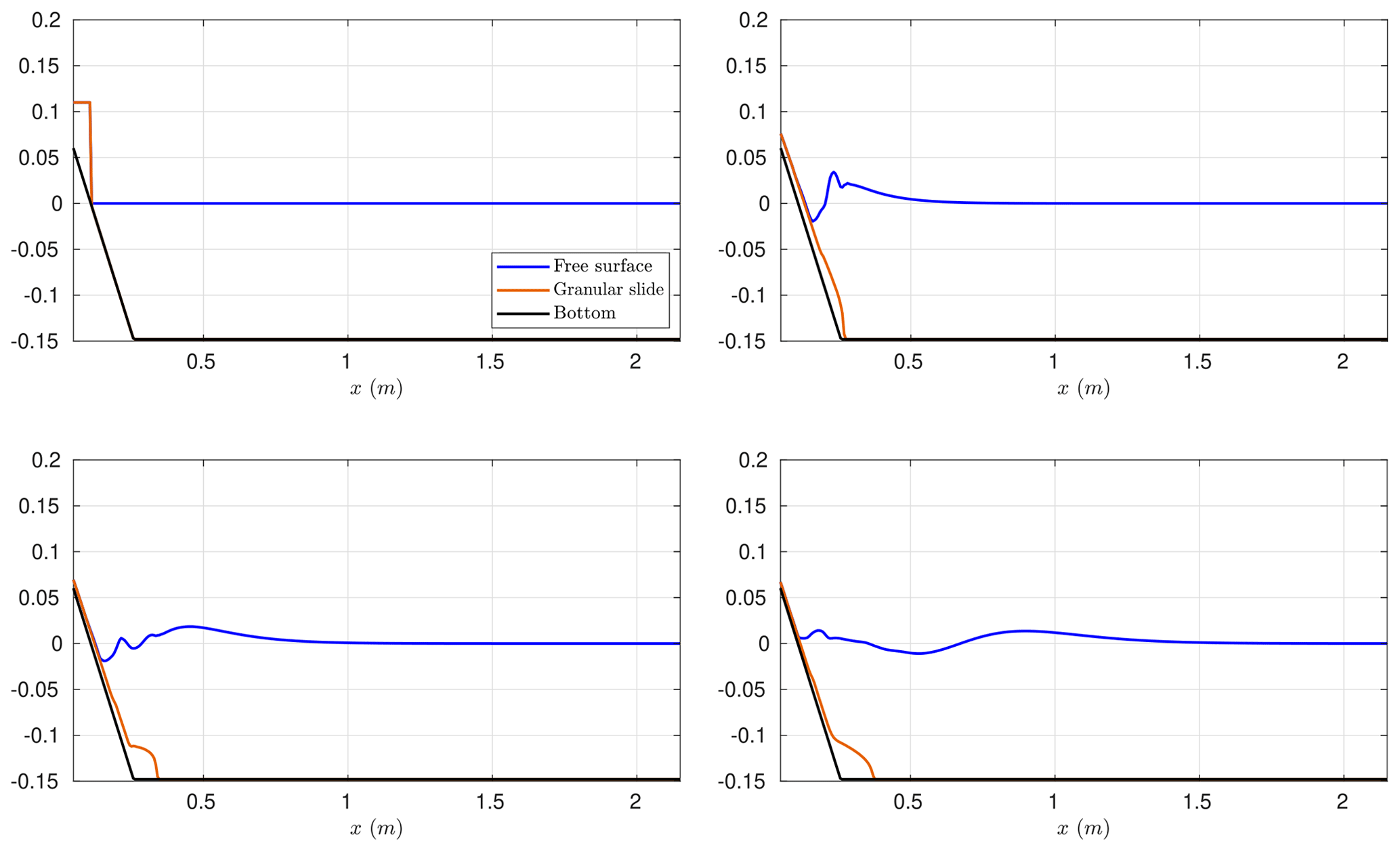
Figure 8Modeled water free-surface elevation and granular slide location at times t=0, 0.2, 0.4, and 0.8 s for Case 1.
5.3 Benchmark problem 6: three-dimensional subaerial granular slide
This benchmark problem is based on the 3D laboratory experiment of Mohammed and Fritz (2012) and Mohammed (2010). Benchmark 6 simulates the rapid entry of a granular slide into a 3D water body. The landslide tsunami experiments were conducted at Oregon State University in Corvallis. The landslides are deployed off a plane with a 27.1∘ slope, as shown in Fig. 9.
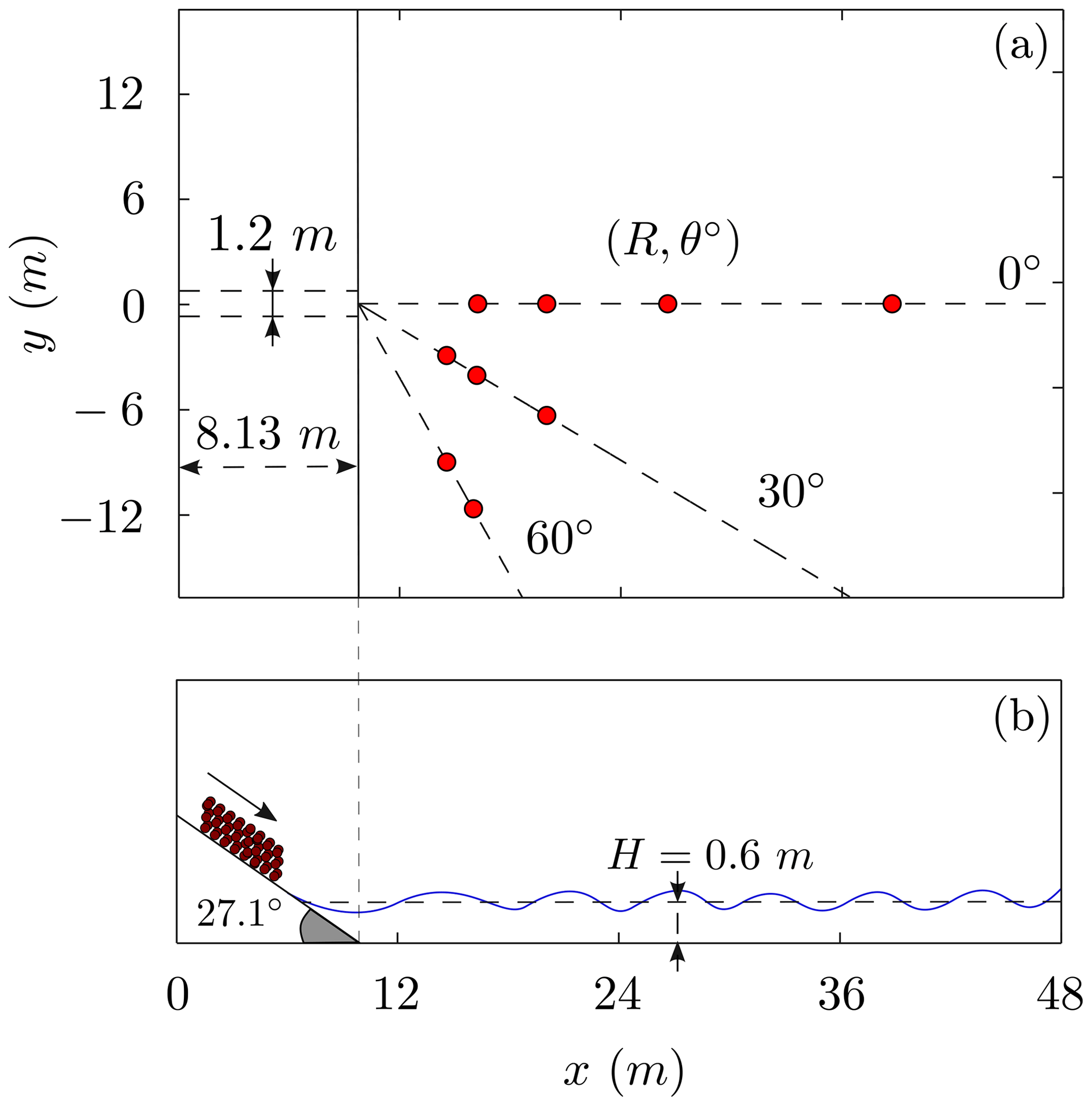
Figure 9Schematic picture of the computational domain. Plan view in panel (a). Cross section at y=0 m in panel (b). The red dots represent the distribution of the wave gauge positions in the laboratory setup.
The landslide material is deployed using a box measuring 2.1 m × 1.2 m × 0.3 m, with a volume of 0.756 m3, and weighting approximately 1360 kg. The case selected by the NTHMP as a benchmarking test is the one with a still-water depth of H=0.6 m (see Fig. 9). The computational domain is the rectangle defined by [0, 48] × [−14, 14], and it is discretized with m. At the boundaries, wall boundary conditions were imposed. The simulation time is 20 s and we set the CFL=0.5. According to Mohammed and Fritz (2012) and Mohammed (2010), the three-dimensional granular landslide parameters were set to
The vertical structure of the fluid layer is modeled using three layers. Similar results were obtained with two layers.
Initially, the slide box is driven using four pneumatic pistons. Here we provide comparisons for the case where the pressure for the pneumatic pistons generating the slide is P=0.4 MPa (P=58 PSI). In Mohammed (2010), it is shown that for this test case, the landslide box reached a velocity of m s−1. Thus, the initial condition for the water velocities is set to zero,
and for the landslide velocity it is set to the above-mentioned constant value,
for the x component. The y component of the landslide velocity was initially set to zero.
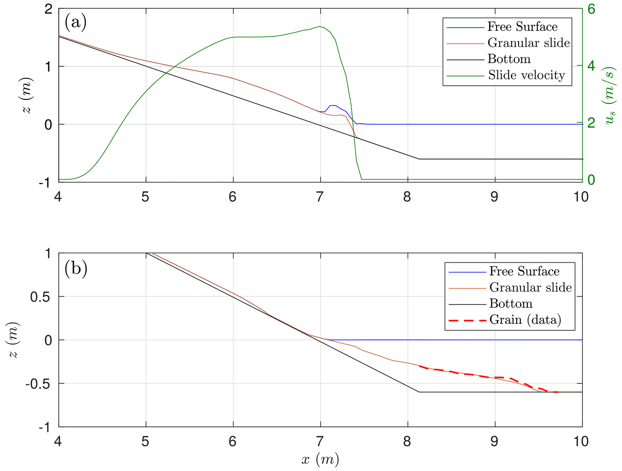
Figure 10BP6 cross section at y=0 m. Panel (a) shows the location and velocity of the granular slide and the generated wave at time t=0.4 s from the triggering and (b) the final deposit location (at t=20 s).

Figure 11Simulated (solid blue lines) time series compared with measured (dashed red lines) free-surface waves for the nine wave gauges considered at (R, θ∘) positions.
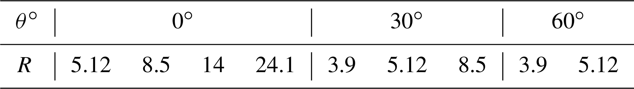
The benchmark problem proposed consists of simulating the free-surface elevation at some wave gauges. In the present study, we include the comparison for the nine wave gauges displayed in Fig. 9 as red dots. A total number of 21 wave gauges composed the whole set of data plus five run-up gauges. The wave gauges in coordinates (R, θ∘) are given more precisely in Table 1.
Table 1Location of the nine waves gauges referenced to the toe's slope.
Before comparing time series, we first check the simulated landslide velocity at impact with the measured one. The slide impact velocity measured in the lab experiment is 5.72 m s−1 at time t=0.44 s. The numerically computed slide impact velocity is slightly underestimated with a value of 5.365 m s−1 at time t=0.4 s as it can be seen in the upper panel of Fig. 10. The final simulated granular deposit is located partially on the final part of the sloping floor and partially at the flat bottom closer to the point of change of slope as is shown in the lower panel of Fig. 10. This can be compared with the actual final location of the granular material in the experimental setup. The simulated deposits, being thinner, extend further. This is probably due to the fact that we are neglecting the friction that it is produced by the change in the slope at the transition area. In Ma et al. (2015) a similar result and discussion can be found.
Figure 11 presents the comparisons between the simulated and the measured waves at the nine gauges we have retained. Model results are in good agreement with measured time. Despite this, wave heights are overestimated at some stations, specially those closer to the shoreline (for example, the station with R=3.9 and θ=30∘). This effect has been also observed and discussed in Ma et al. (2015). At some of the time series, it can be observed that the small free-surface oscillations at the final part of the time series are not well captured by the model. This is partially due to the relatively coarse horizontal grids used in the simulation. This same behavior can be also observed in Fig. 12 in this case for the comparisons between the simulated and measured run-up values at some measure locations situated at the shoreline (as for x=7.53).
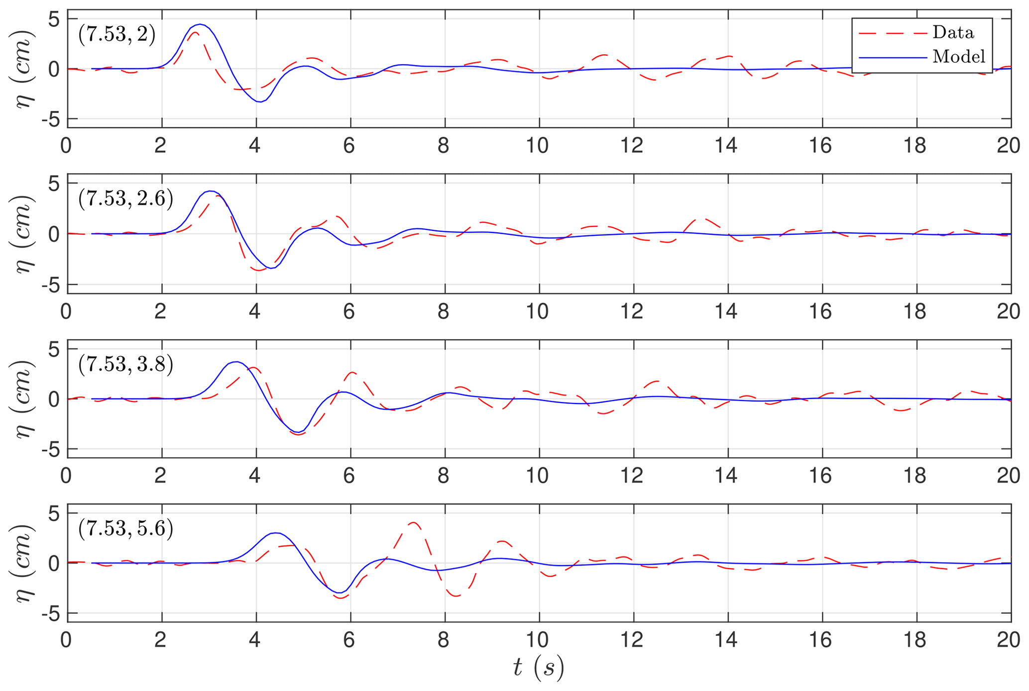
Figure 12Time series comparing numerical run-up (solid blue) at the four run-up gauges with the measured (dashed red) data at (x, y) positions.
Table 2Wall-clock times in seconds for the hydrostatic shallow-water Savage–Hutter system (SWE-SH) and the non-hydrostatic GPU implementations. The ratios are with respect to the SWE-SH model implementation.
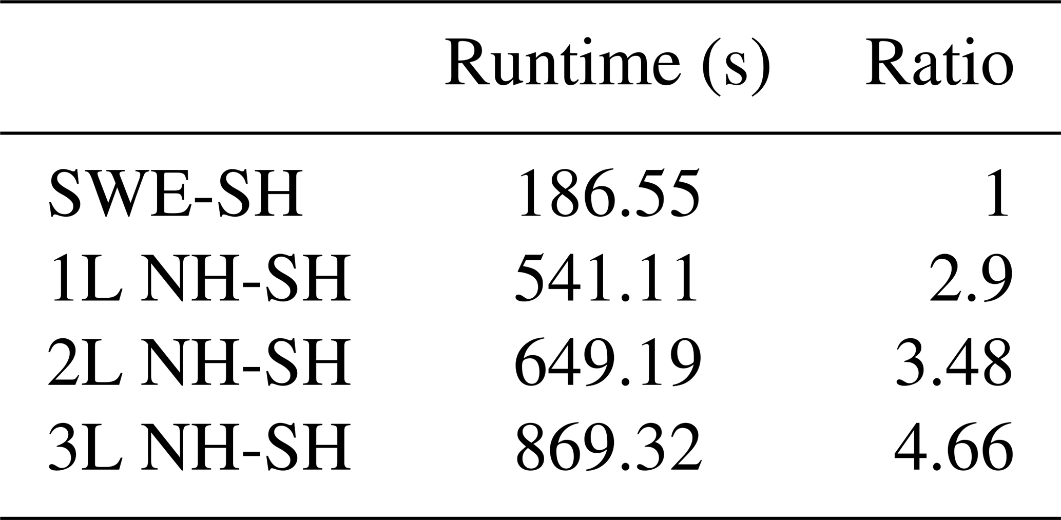
Table 2 shows the wall-clock times on an NVIDIA Tesla P100 GPU. It can be observed that including non-hydrostatic terms in the SWE-SH system results in an increase in the computational time of 2.9 times. If a richer vertical structure is considered, then larger computational times are required. As in the examples for the two- and three-layer systems, there is a 3.48 and 4.66 times increase in the computational effort.
Numerical models need to be validated prior to their use as predictive tools. This requirement becomes even more necessary when these models are going to be used for risk assessment in natural hazards where human lives are involved. The current work aims at benchmarking the novel Multilayer-HySEA model for landslide-generated tsunamis produced by granular slides, in order to provide the tsunami community with a robust, efficient, and reliable tool for landslide tsunami hazard assessment in the future.
The Multilayer-HySEA code implements a two-phase model to describe the interaction between landslides (aerial or subaerial) and water body. The upper phase describes the hydrodynamic component. This is done using a stratified vertical structure that includes non-hydrostatic terms in order to include dispersive effects in the propagation of simulated waves. The motion of the landslide is taken into account by the lower phase, consisting of a Savage–Hutter model. To reproduce these flows, the friction model given in Pouliquen and Forterre (2002) is considered here. The hydrodynamic and morphodynamic models are weakly coupled through the boundary condition at their interface.
The implemented numerical algorithm combines a finite-volume path-conservative scheme for the underlying hyperbolic system and finite differences for the discretization of the non-hydrostatic terms. The numerical model is implemented to be run in GPU architectures. The two-layer non-hydrostatic code coupled with the Savage–Hutter used here has been shown to run at very efficient computational times. To assess this, we compare with respect to the one-layer SWE/Savage–Hutter GPU code. For the numerical simulations performed here, the execution times for the non-hydrostatic model are always below 4.66 times the times for the SWE model for a number of layers up to three. We can conclude that the numerical scheme presented here is very robust, is extremely efficient, and can model dispersive effects generated by submarine/subaerial landslides at a low computational cost considering that dispersive effects and a vertical multilayer structure are included in the model. Model results show a good agreement with the experimental data for the three benchmark problems considered, in particular for BP5, but this also occurs for the other two benchmark problems. In general, a better agreement for the hydrodynamic component, compared with its morphodynamic counterpart, is shown, which is more challenging to reproduce.
The numerical code is currently under development and only available to close collaborators. In the future, we will provide an open version of the code as we already do for Tsunami-HySEA. This version will be available from the website https://edanya.uma.es/hysea/ (last access: 21 February 2021) (Macías, 2021). Finally, the NetCDF files containing the numerical results obtained with the Multilayer-HySEA code for all the tests presented here can be found and download from Macías et al. (2020b).
All the data used in the present work and necessary to reproduce the setup of the numerical experiments as well as the laboratory-measured data to compare with can be downloaded from LTMBW (2017) at http://www1.udel.edu/ kirby/landslide/ (last access: 21 February 2021).
JM led the HySEA codes benchmarking effort undertaken by the EDANYA group, wrote most of the paper, reviewed and edited it, and assisted in the numerical experiments and in their setup. CE implemented the numerical code and performed all the numerical experiments; he also contributed to the writing of the manuscript. JM and CE did all the figures. MC significantly contributed to the design and implementation of the numerical code.
The authors declare that they have no conflict of interest.
The authors are indebted to Diego Arcas (PMEL/NOAA) and Victor Huérfano (PRSN) for supporting our participation in the 2017 Galveston workshop and to the MMS of the NTHMP for kindly inviting us to that event.
This research has been supported by the Spanish Government–FEDER (project MEGAFLOW) (grant no. RTI2018-096064-B-C21) and the Junta de Andalucía–FEDER (grant no. UMA18-Federja-161).
This paper was edited by Maria Ana Baptista and reviewed by two anonymous referees.
Abadie, S., Morichon, D., Grilli, S., and Glockner, S.: Numerical simulation of waves generated by landslides using a multiple-fluid Navier–Stokes model, Coast. Eng., 57, 779–794, https://doi.org/j.coastaleng.2010.03.003, 2010. a
Abadie, S. M., Harris, J. C., Grilli, S. T., and Fabre, R.: Numerical modeling of tsunami waves generated by the flank collapse of the Cumbre Vieja Volcano (La Palma, Canary Islands): Tsunami source and near field effects, J. Geophys. Res.-Oceans, 117, C05030, https://doi.org/10.1029/2011JC007646, 2012. a
Adsuara, J., Cordero-Carrión, I., Cerdá-Durán, P., and Aloy, M.: Scheduled relaxation Jacobi method: Improvements and applications, J. Comput. Phys., 321, 369–413, https://doi.org/10.1016/j.jcp.2016.05.053, 2016. a
Ataie-Ashtiani, B. and Najafi-Jilani, A.: Laboratory investigations on impulsive waves caused by underwater landslide, Coast. Eng., 55, 989–1004, https://doi.org/10.1016/j.coastaleng.2008.03.003, 2008. a, b
Ataie-Ashtiani, B. and Shobeyri, G.: Numerical simulation of landslide impulsive waves by incompressible smoothed particle hydrodynamics, Int. J. Numer. Meth. Fluids, 56, 209–232, https://doi.org/10.1002/fld.1526, 2008. a
Brunet, M., Moretti, L., Le Friant, A., Mangeney, A., Fernández Nieto, E. D., and Bouchut, F.: Numerical simulation of the 30–45 ka debris avalanche flow of Montagne Pelée volcano, Martinique: from volcano flank collapse to submarine emplacement, Nat. Hazards, 87, 1189–1222, 2017. a, b
Castro, M. and Fernández-Nieto, E.: A class of computationally fast first order finite volume solvers: PVM methods, SIAM J. Scient. Comput., 34, A2173–A2196, 2012. a
Castro, M., Ortega, S., de la Asunción, M., Mantas, J., and Gallardo, J.: GPU computing for shallow water flow simulation based on finite volume schemes, Comptes Rendus Mécanique, 339, 165–184, 2011. a
Escalante, C., Fernández-Nieto, E., Morales, T., and Castro, M.: An efficient two–layer non-hydrostatic approach for dispersive water waves, J. Scient. Comput., 79, 273–320, https://doi.org/10.1007/s10915-018-0849-9, 2018a. a, b, c
Escalante, C., Morales, T., and Castro, M.: Non-hydrostatic pressure shallow flows: GPU implementation using finite volume and finite difference scheme, Appl. Math. Comput., 338, 631–659, https://doi.org/10.1016/j.amc.2018.06.035, 2018b. a, b, c
Fernández-Nieto, E., Bouchut, F., Bresch, D., Castro, M., and Mangeney, A.: A new Savage-Hutter type model for submarine avalanches and generated tsunami, J. Comput. Phys., 227, 7720–7754, 2008. a
Fernández-Nieto, E., Parisot, M., Penel, Y., and Sainte-Marie, J.: A hierarchy of dispersive layer-averaged approximations of Euler equations for free surface flows, Commun. Math. Sci., 16, 1169–1202, 2018. a, b, c, d
Ferreiro-Ferreiro, A., García-Rodríguez, J., López-Salas, J., Escalante, C., and Castro, M.: Global optimization for data assimilation in landslide tsunami models, J. Comput. Phys., 403, 109069, https://doi.org/10.1016/j.jcp.2019.109069, 2020. a
Fine, I. V., Rabinovich, A. B., and Kulikov, E. A.: Numerical modelling of landslide generated tsunamis with application to the Skagway Harbor tsunami of November 3, 1994, in: Proc. Intl. Conf. on Tsunamis, Paris, 211–223, 1998. a
Fritz, H. M., Hager, W. H., and Minor, H.-E.: Near field characteristics of landslide generated impulse waves, J. Waterway Port Coast. Ocean Eng., 130, 287–302, https://doi.org/10.1061/(ASCE)0733-950X(2004)130:6(287), 2004. a
Garres-Díaz, J., Fernández-Nieto, E. D., Mangeney, A., and de Luna, T. M.: A weakly non-hydrostatic shallow model for dry granular flows, J. Scient. Comput., 86, https://doi.org/10.1007/s10915-020-01377-9, 2021. a, b, c
González-Vida, J., Macías, J., Castro, M., Sánchez-Linares, C., Ortega, S., and Arcas, D.: The Lituya Bay landslide-generated mega-tsunami. Numerical simulation and sensitivity analysis, Nat. Hazards Earth Syst. Sci., 19, 369–388, https://doi.org/10.5194/nhess-19-369-2019, 2019. a, b, c, d
Grilli, S. T., Shelby, M., Kimmoun, O., Dupont, G., Nicolsky, D., Ma, G., Kirby, J. T., and Shi, F.: Modeling coastal tsunami hazard from submarine mass failures: effect of slide rheology, experimental validation, and case studies off the US East Coast, Nat. Hazards, 86, 353–391, https://doi.org/10.1007/s11069-016-2692-3, 2017. a, b, c, d
Harbitz, C. B., Pedersen, G., and Gjevik, B.: Numerical simulations of large water waves due to landslides, J. Hydraul. Eng., 119, 1325–1342, https://doi.org/10.1061/(ASCE)0733-9429(1993)119:12(1325), 1993. a
Heinrich, P.: Nonlinear water waves generated by submarine and aerial landslides, J. Waterway Port Coast. Ocean Eng., 118, 249–266, https://doi.org/10.1061/(ASCE)0733-950X(1992)118:3(249), 1992. a
Heller, V. and Hager, W.: Impulse product parameter in landslide generated impulse waves, J. Waterway Port Coast. Ocean Eng., 136, 145–155, https://doi.org/10.1061/(ASCE)WW.1943-5460.0000037, 2010. a
Horrillo, J., Wood, A., Kim, G.-B., and Parambath, A.: A simplified 3-D Navier–Stokes numerical model for landslide-tsunami: Application to the Gulf of Mexico, J. Geophys. Res.-Oceans, 118, 6934–6950, https://doi.org/10.1002/2012JC008689, 2013. a
Kirby, J. T., Shi, F., Nicolsky, D., and Misra, S.: The 27 April 1975 Kitimat, British Columbia, submarine landslide tsunami: a comparison of modeling approaches, Landslides, 13, 1421–1434, https://doi.org/10.1007/s10346-016-0682-x, 2016. a, b
Kirby, J. T., Grilli, S. T., Zhang, C., Horrillo, J., Nicolsky, D., and Liu, P. L.-F.: The NTHMP Landslide Tsunami Benchmark Workshop, Galveston, January 9–11, 2017, Tech. rep., Research Report CACR-18-01, available at: http://www1.udel.edu/kirby/landslide/report/kirby-etal-cacr-18-01.pdf (last access: 20 February 2021), 2018. a, b, c
LTMBW: Landslide Tsunami Model Benchmarking Workshop, Galveston, Texas, 2017, available at: http://www1.udel.edu/kirby/landslide/index.html (last access: 21 April 2020), 2017. a, b
Ma, G., Shi, F., and Kirby, J. T.: Shock-capturing non-hydrostatic model for fully dispersive surface wave processes, Ocean Model., 43–44, 22–35, https://doi.org/10.1016/j.ocemod.2011.12.002, 2012. a
Ma, G., Kirby, J. T., and Shi, F.: Numerical simulation of tsunami waves generated by deformable submarine landslides, Ocean Model., 69, 146–165, https://doi.org/10.1016/j.ocemod.2013.07.001, 2013. a
Ma, G., Kirby, J. T., Hsu, T.-J., and Shi, F.: A two-layer granular landslide model for tsunami wave generation: Theory and computation, Ocean Model., 93, 40–55, https://doi.org/10.1016/j.ocemod.2015.07.012, 2015. a, b, c
Macías, J.: HySEA codes web page, available at: https://edanya.uma.es/hysea/, last access: 21 February 2021. a
Macías, J., Vázquez, J., Fernández-Salas, L., González-Vida, J., Bárcenas, P., Castro, M., del Río, V. D., and Alonso, B.: The Al-Borani submarine landslide and associated tsunami. A modelling approach, Mar. Geol., 361, 79–95, https://doi.org/10.1016/j.margeo.2014.12.006, 2015. a, b
Macías, J., Castro, M., Ortega, S., Escalante, C., and González-Vida, J.: Performance Benchmarking of Tsunami-HySEA Model for NTHMP's Inundation Mapping Activities, Pure Appl. Geophys., 174, 3147–3183, https://doi.org/10.1007/s00024-017-1583-1, 2017. a
Macías, J., Escalante, C., Castro, M., González-Vida, J., and Ortega, S.: HySEA model, Landslide Benchmarking Results, NTHMP report, Tech. rep., Universidad de Málaga, Málaga, https://doi.org/10.13140/RG.2.2.27081.60002, 2017. a, b
Macías, J., Escalante, C., and Castro, M.: Performance assessment of Tsunami-HySEA model for NTHMP tsunami currents benchmarking. Laboratory data, Coast. Eng., 158, 103667, https://doi.org/10.1016/j.coastaleng.2020.103667, 2020a. a
Macías, J., Escalante, C., and Castro, M.: Numerical results in Multilayer-HySEA model validation for landslide generated tsunamis. Part II Granular slides, Dataset on Mendeley, https://doi.org/10.17632/94txtn9rvw.2, 2020b. a
Macías, J., Ortega, S., González-Vida, J., and Castro, M.: Performance assessment of Tsunami-HySEA model for NTHMP tsunami currents benchmarking. Field cases, Ocean Model., 152, 101645, https://doi.org/10.1016/j.ocemod.2020.101645, 2020c. a
Macías, J., Escalante, C., and Castro, M. J.: Multilayer-HySEA model validation for landslide-generated tsunamis – Part 1: Rigid slides, Nat. Hazards Earth Syst. Sci., 21, 775–789, https://doi.org/10.5194/nhess-21-775-2021, 2021. a, b, c, d
Mangeney, A., Bouchut, F., Thomas, N., Vilotte, J. P., and Bristeau, M. O.: Numerical modeling of self-channeling granular flows and of their levee-channel deposits, J. Geophys. Res.-Earth, 112, F02017, https://doi.org/10.1029/2006JF000469, 2007. a, b
Mohammed, F.: Physical modeling of tsunamis generated by three-dimensional deformable granular landslides, PhD thesis, Georgia Institute of Technology, Atlanta, GA, USA, 2010. a, b, c
Mohammed, F. and Fritz, H. M.: Physical modeling of tsunamis generated by three-dimensional deformable granular landslides, J. Geophys. Res.-Oceans, 117, C11015, https://doi.org/10.1029/2011JC007850, 2012. a, b, c, d
Pouliquen, O. and Forterre, Y.: Friction law for dense granular flows: application to the motion of a mass down a rough inclined plane, J. Fluid Mech., 453, 133–151, https://doi.org/10.1017/S0022112001006796, 2002. a, b, c, d, e, f
Rzadkiewicz, S. A., Mariotti, C., and Heinrich, P.: Numerical simulation of submarine landslides and their hydraulic effects, J. Waterway Port Coast. Ocean Eng., 123, 149–157, https://doi.org/10.1061/(ASCE)0733-950X(1997)123:4(149), 1997. a, b
Sánchez-Linares, C., de la Asunción, M., Castro, M., Vida, J. G., Macías, J., and Mishra, S.: Uncertainty quantification in tsunami modeling using multi-level Monte Carlo finite volume method, J. Math. Indust., 6, 5, https://doi.org/10.1186/s13362-016-0022-8, 2016. a
Savage, S. and Hutter, K.: The motion of a finite mass of granular material down a rough incline, J. Fluid Mech., 199, 177–215, https://doi.org/10.1017/S0022112089000340, 1989. a
Viroulet, S., Sauret, A., and Kimmoun, O.: Tsunami generated by a granular collapse down a rough inclined plane, Europhys. Lett., 105, 34004, https://doi.org/10.1209/0295-5075/105/34004, 2014. a, b, c, d, e
Weiss, R., Fritz, H. M., and Wünnemann, K.: Hybrid modeling of the mega-tsunami runup in Lituya Bay after half a century, Geophys. Res. Lett., 36, L09602, https://doi.org/10.1029/2009GL037814, 2009. a
Yavari-Ramshe, S. and Ataie-Ashtiani, B.: Numerical modeling of subaerial and submarine landslide-generated tsunami waves–recent advances and future challenges, Landslides, 13, 1325–1368, https://doi.org/10.1007/s10346-016-0734-2, 2016. a
- Abstract
- Introduction
- The Landslide-HySEA model for granular slides
- The Multilayer-HySEA model
- Numerical solution method
- Benchmark problem comparisons
- Concluding remarks
- Code availability
- Data availability
- Author contributions
- Competing interests
- Acknowledgements
- Financial support
- Review statement
- References