the Creative Commons Attribution 4.0 License.
the Creative Commons Attribution 4.0 License.
 | 26 Feb 2021
Multilayer-HySEA model validation for landslide-generated tsunamis – Part 1: Rigid slides
Cipriano Escalante
Manuel J. Castro
This paper is devoted to benchmarking the Multilayer-HySEA model using laboratory experimental data for landslide-generated tsunamis. This article deals with rigid slides, and the second part, in a companion paper, addresses granular slides. The US National Tsunami Hazard and Mitigation Program (NTHMP) has proposed the experimental data used and established for the NTHMP Landslide Benchmark Workshop, held in January 2017 at Galveston (Texas). The first three benchmark problems proposed in this workshop deal with rigid slides. Rigid slides must be simulated as a moving bottom topography, and, therefore, they must be modeled as a prescribed boundary condition. These three benchmarks are used here to validate the Multilayer-HySEA model. This new HySEA model consists of an efficient hybrid finite-volume–finite-difference implementation on GPU architectures of a non-hydrostatic multilayer model. A brief description of model equations, dispersive properties, and the numerical scheme is included. The benchmarks are described and the numerical results compared against the lab-measured data for each of them. The specific aim is to validate this new code for tsunamis generated by rigid slides. Nevertheless, the overall objective of the current benchmarking effort is to produce a ready-to-use numerical tool for real-world landslide-generated tsunami hazard assessment. This tool has already been used to reproduce the Port Valdez, Alaska, 1964 and Stromboli, Italy, 2002 events.
- Article
(3299 KB) - Full-text XML
- Companion paper
- BibTeX
- EndNote


Model development and benchmarking for earthquake-induced tsunamis is a task addressed in the past and to which much effort and time has been dedicated. In particular, just to mention a couple of NTHMP efforts, the 2011 Galveston benchmarking workshop (Horrillo et al., 2015) and the 2015 Portland workshop for tsunami currents (Lynett et al., 2017) both focused on these topics. However, both model development and benchmarking efforts have advanced at a slower pace for landslide-generated tsunamis. As examples we might mention the 2003 NSF-sponsored landslide tsunami workshop organized in Hawaii and a similar follow-up workshop on Catalina Island in 2006 (Liu et al., 2008). Since then, no similar large comprehensive benchmarking workshop has been organized (Kirby et al., 2018).
In its 2019 strategic plan, the NTHMP required that all numerical tsunami inundation models to be used in hazard assessment studies in the United States be verified as accurate and consistent through a model benchmarking process. This mandate was fulfilled in 2011 but only for seismic tsunami sources and to a limited extent for idealized solid underwater landslides. However, recent work by various NTHMP states has shown that landslide tsunami hazard may in fact be greater than seismically induced hazard and may be also the dominant risk along significant parts of the US coastline (ten Brink et al., 2014).
As a result of this demonstrated gap, a set of candidate benchmarks was proposed to perform the required validation process. The selected benchmarks are based on a subset of available laboratory data sets for solid slide experiments and deformable slide experiments and include both submarine and subaerial slides. In order to complete this list of laboratory data, a benchmark based on a historic field event (Valdez, AK, 1964) was also chosen. The EDANYA group (https://www.uma.es/edanya, last access: 18 February 2021) from the University of Málaga participated in the workshop organized at Texas A&M University, Galveston (9–11 January 2017), presenting results for the benchmarking tests with two numerical codes: Landslide-HySEA and Multilayer-HySEA models. At Galveston, we presented numerical results for six out of the seven benchmark problems proposed, including the field case. The current work presents the numerical results obtained for the Multilayer-HySEA model in the framework of the validation effort described above for the case of rigid-slide-generated tsunamis, whereas the benchmark problems dealing with granular slides are presented in a companion paper, Macías et al. (2021). A summary of the results for the field case at Port Valdez can be found in Macías et al. (2017).
Twenty years ago, at the beginning of the century, the challenge of solid block landslide modeling was taken by a number of researchers (Grilli and Watts, 1999, 2005; Grilli et al., 2002; Lynett and Liu, 2002; Watts et al., 2003, 2005; Wu, 2004; Liu et al., 2005), and laboratory experiments were developed for those cases and for tsunami model benchmarking (Enet and Grilli, 2007) (see also Ataie-Ashtiani and Najafi-Jilani, 2008). The benchmark problems (BPs) performed in the current work are based on the laboratory experiments of Grilli and Watts (2005) for BP1, Enet and Grilli (2007) for BP2, and Wu (2004) and Liu et al. (2005) for BP3. The basic reference for these three benchmarks, as well as for the three benchmarks related to granular slides and the Alaska field case (all of them proposed by the NTHMP), is Kirby et al. (2018). We highly recommend checking this reference for further details on benchmark descriptions, data provided for performing them, required benchmark items, and inter-model comparison. Finally, we would like to stress that the ultimate goal of our current benchmarking effort is to provide the tsunami community with an NTHMP-approved model for landslide-generated tsunami hazard assessment, similarly to what we have done with the Tsunami-HySEA model for the case of earthquake-generated tsunamis (Macías et al., 2017, 2020a, c).
The HySEA (Hyperbolic Systems and Efficient Algorithms) software consists of a family of geophysical codes based on either single-layer, two-layer stratified systems, or multilayer shallow-water models. HySEA codes1 have been under development by the EDANYA group from UMA (the University of Málaga) for more than a decade. These codes are in continuous evolution and undergo continuous upgrading, and they serve a wider scientific community every day. The first model we developed dealing with landslide-generated tsunamis consisted of a stratified two-layer Savage–Hutter shallow-water model – the Landslide-HySEA model. It was implemented based on the model described in Fernández et al. (2008) and was incorporated into the HySEA family. An initial validation of this code, comparing numerical results with the laboratory experiments of Heller and Hager (2011) and Fritz et al. (2001), can be found in Sánchez-Linares (2011). The 2018 numerical simulation of the 1958 Lituya Bay mega-tsunami with real topo-bathymetric data and encouraging results (González-Vida et al., 2019) represented a milestone in the verification process of this code. This validation effort was accomplished under a research contract with the NOAA Pacific Marine Environmental Laboratory (PMEL). The result of this project led the NCTR (NOAA Center for Tsunami Research) to adopt Landslide-HySEA as the numerical code of choice to generate the initial conditions for the MOST model to be initialized in the case of a landslide-generated tsunami scenario to be simulated. Further applications of Landslide-HySEA can be found in de la Asunción et al. (2013), Macías et al. (2015), and Iglesias (2015).
The waves generated in the laboratory tests proposed in the NTHMP selected benchmarks are high frequency and dispersive, and the generated flows have a complex vertical structure. Therefore, the numerical model used must be able to reproduce such effects. This makes the two-layer Landslide-HySEA model unsuitable for reproducing these experimental results as non-hydrostatic effects play an important role and a richer vertical structure is required. To address these requirements, the Multilayer-HySEA model was very recently implemented, considering a stratified structure in the simulated fluid and including non-hydrostatic terms. A multilayer model is able to better approximate the vertical structure of a complex flow than a standard one-layer depth-averaged model. In particular, by increasing the number of layers, the linear dispersion relation of the model converges towards the exact dispersion relation from the Stokes linear theory (see Fernández-Nieto et al., 2018).
The Multilayer-HySEA model implements one of the multilayer non-hydrostatic models of the family introduced and described in Fernández-Nieto et al. (2018) (model LDNH0). The governing equations, which are obtained by a process of depth averaging, correspond to a semi-discretization for the vertical variable of the Euler equations following a standard Galerkin approach. The total pressure is decomposed into a sum of hydrostatic and non-hydrostatic pressures and is assumed to have a linear vertical profile. The horizontal and vertical velocities are assumed to have a constant vertical profile. At the discrete level on z, the total pressure matches at the interfaces and velocities satisfy a discrete jump condition (see Fernández et al., 2008, or Escalante et al., 2018a).
An alternative deduction for this system is performed in Escalante et al. (2018a) assuming linear vertical profiles for pressure and vertical velocity and a constant vertical profile for the horizontal velocity, as well as some extra hypotheses for the case of two layers. The proposed model admits an exact energy balance, and, when the number of layers increases, the linear dispersion relation of the linear model converges to that of Airy's theory (Fernández-Nieto et al., 2018). The model proposed in Fernández-Nieto et al. (2018) can be written in a compact form as
where, for , the following notation is used:
where f denotes one of the generic variables of the system, i.e., u, w, and p, and, finally,

Total depth, h, is split along the vertical axis into L≥1 layers and (see Fig. 1). The variables uα and wα are the depth-averaged velocities in the x and z directions, respectively, t is time, and g is gravitational acceleration. The non-hydrostatic pressure at the interface is denoted by . The water surface elevation measured from the still-water level is , where H is the water depth when the water is at rest. Finally, τ is a friction law term, and the terms account for the mass transfer across interfaces and are defined by
In order to close the system of equations, the following boundary conditions are considered:
Note that the motion of the bottom surface can be taken into account as a boundary condition, imposing w0≠0. Therefore, this model can simulate the interaction with a slide in the case that the motion of the bottom is prescribed by a function, given by a set of data, or simulated by a numerical model. In the present study, we are going to consider tests where the motion of the seafloor is given by a known function (the solid moving block).
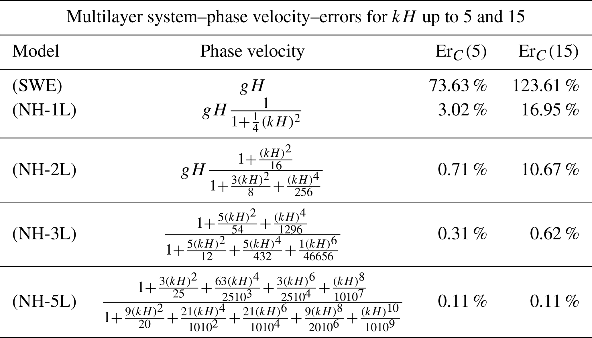
Table 1Phase velocity expressions and maximum of the relative error ErC(s) compared with Airy's theory for different ranges of for the non-linear hydrostatic shallow-water system (SWE) and the Multilayer-HySEA (non-hydrostatic) system with j≥1 layers (NH–jL).
3.1 Linear dispersion relation
Some dispersive properties of the system (Eq. 1) are presented in this section, in particular, the phase and group velocities, as well as the linear shoaling. The first two properties are related to the propagation of dispersive wave trains and the last one to shoaling processes.
To obtain such properties, system Eq. (1) is linearized around the water-at-rest steady-state solution. After that, a Stokes-type Fourier analysis is carried out looking for first-order planar wave solutions. This method constitutes a standard procedure to study systems that model dispersive water waves (see Escalante et al., 2018a; Lynett and Liu, 2004; Madsen and Sorensen, 1992; Schäffer and Madsen, 1995, and references therein). The phase and group velocities as well as the linear shoaling gradient are, respectively, defined as
where ω denotes the angular frequency, k the local wave number, and H the typical depth.
The measured quantities C, G, and γ are solely functions of the local wave number and the typical depth H. Thus, one can obtain the so-called linear dispersion relation of the three measured quantities. From the Airy wave theory, one can also obtain the corresponding linear dispersion relations that state the linear theory for the considered quantities (see Schäffer and Madsen, 1995, for the Airy reference formulae). For example, the expression for the phase velocity from Airy's theory is
The expressions of the phase velocity for the system (Eq. 1) are given in Table 1 for the non-linear hydrostatic shallow-water system (SWE) and the Multilayer-HySEA (non-hydrostatic) system with j≥1 layers (NH–jL). The last two columns contain ErC(s) for s=5 and s=15, where ErC(s) represents the maximum relative error of the phase velocity with respect to the Airy in a range in percent, i.e.,
The main goal when deriving dispersive shallow-water systems is to get the most accurate dispersive relations as possible, compared with the Airy wave theory, without highly increasing the complexity of the system. See Schäffer and Madsen (1995) for a review on state-of-the-art dispersive models or a two-layer model with improved dispersive relations in Lynett and Liu (2004), as well as an enhanced two-layer non-hydrostatic pressure system in Escalante et al. (2018a). It has been shown (Fernández-Nieto et al., 2018) that increasing the number of layers leads to the convergence of the linear dispersion relation of the linear model to that of Airy's theory. Figure 2 shows this behavior and highlights the huge discrepancies between Airy's theory and the systems (SWE) and (NH-1L). It is well known that waves generated by landslides might present high characteristic values for kH. For the (SWE) system, it is well known that it has an accurate phase velocity in a small range of kH and that this system is appropriate for long waves as tsunami waves but not for dispersive waves with higher values of kH. In the same vein, the one-layer non-hydrostatic pressure system (NH-1L) can improve these results, but, again, poor linear dispersive results are achieved in a range of kH between 5 and 15. However, when the number of layers, L, is set to 3 (still a small value) the (Eq. 1) is in an excellent agreement with the Airy theory for kH up to 15. For the phase celerity, the percentage error is less than 0.62 %, and for the group velocity it is less than 1 % for kH smaller than 10 (see Fig. 2). Linear shoaling is also well reproduced in this same range.
The Multilayer-HySEA model presents enhanced dispersive properties. In order to have similar dispersive results as the ones obtained here using a three-layer system, at least five layers are required for other similar multilayer models as the one presented in Bai and Cheung (2018). Furthermore, the results presented for the phase velocity with two layers in Table 1 show that the system proposed here produces smaller relative error for kH up to 15 compared with the two-layer system in Cui et al. (2014). That means that the Multilayer-HySEA model can achieve better dispersive properties than models having similar or even more computational complexity.
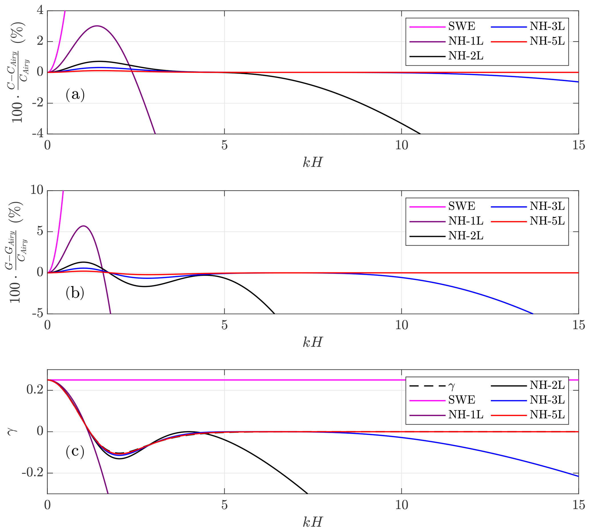
Figure 2Relative error for the phase velocities (a), the group velocities (b), and comparison with the reference shoaling gradient (c), with respect to the Airy theory for the described multilayer systems (2L, 3L, and 5L), the one-layer non-hydrostatic, and the shallow-water system.
3.2 Modeling of breaking waves and wetting and drying treatment
3.2.1 Modeling of breaking waves
In shallow areas the breaking of waves can be observed near the coast. As pointed out in Escalante et al. (2018a, b, 2019) and Roeber et al. (2010) among others, non-hydrostatic partial-differential-equation (PDE) systems such as the one considered in this paper cannot describe this process without the inclusion of an additional term that accounts for the dissipation of the amount of energy required when breaking phenomena occur. In this work, we have implemented a simplified generalization of the breaking mechanism that was introduced in Escalante et al. (2018a) for the case of two layers. To do so, the vertical component of the stress tensor is depth-averaged on the vertical variable. Thus, adding the proposed integrated viscosity term to system Eq. (1), only the vertical momentum equation changes and reads for each as
where is the eddy viscosity. In this work, as in Escalante et al. (2018a) and Roeber et al. (2010), we choose ς to be
where B is an empirical parameter related to a breaking criteria to switch on and off this extra dissipation term. The definition of this empirical parameter is based on a quasi-heuristic strategy to determine when the breaking occurs (see Escalante et al., 2018b; Roeber et al., 2010, and references therein).
Finally, a natural and simple extension of the criterion proposed by Roeber et al. (2010) is adopted
where
denote the flow speed at the onset and termination of the wave-breaking process and B1 and B2 are calibration coefficients. In this work, we use B1=0.6 and B2=0.15 for all the test cases studied. Finally, depending on the benchmark problem, we use
3.2.2 Wetting and drying treatment
For the computation of variables in areas of small water depth, a wet–dry treatment adapting the ideas described in Castro et al. (2005) is applied. The key elements for the numerical treatment of wet–dry fronts with emerging bottom topographies are based on the following.
-
The hydrostatic pressure terms at the horizontal velocity equations are modified for emerging bottoms to avoid spurious pressure forces (see Castro et al., 2005).
-
To overcome the difficulties due to large round-off errors in computing the velocities uα,wα from discharges for small values of h, we define the velocities analogously as in Kurganov and Petrova (2007), applying the desingularization formula
which gives the exact value of uα and wα for h≥ϵ and gives a smooth transition of uα and wα to zero when h tends to zero without truncation. In this work we set for the numerical tests. A more detailed discussion about the desingularization formula can be seen in Kurganov and Petrova (2007).
We describe now the discretization of system Eq. (1) that follows the natural extension of the procedure described in Escalante et al. (2018a, b) for the one- and two-layer non-hydrostatic system. The numerical scheme employed is based on a two-step projection-correction method, similar to the standard Chorin projection method for Navier–Stokes equations (Chorin, 1968). This is a standard procedure when dealing with dispersive systems (see Escalante et al., 2018a, b; Ma et al., 2012; Kazolea and Delis, 2013; Ricchiuto and Filippini, 2014, and references therein).
First, we shall solve the non-conservative hyperbolic underlying shallow-water (SW) system (Eq. 1) given by the compact equation
where the following compact notation has been used:
and BSW is a matrix such that BSW∂xU contains the non-conservative products related to the mass transfer across interfaces appearing at the momentum equations.
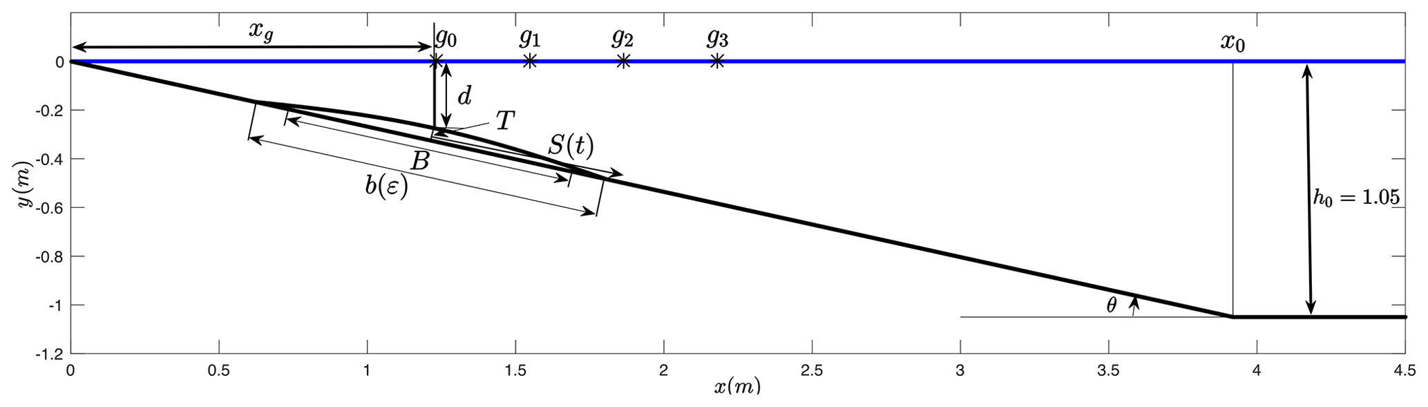
Figure 3BP1. Sketch of main parameters and variables for wave generation by 2D rigid slide (modified from Grilli and Watts, 2005).
Then, in a second step, non-hydrostatic terms given by the pressure vector correction term
as well as the divergence constraints at each layer
will be taken into account.
System Eq. (14) is discretized using a second-order finite-volume polynomial-viscosity-matrix (PVM) positive-preserving well-balanced path-conservative method (Castro and Fernández-Nieto, 2012). As usual, we consider a set of N finite-volume cells with constant lengths Δx and define
the cell average of the function U(x,t) on cell Ii at time t. Concerning non-hydrostatic terms, we consider midpoints xi of each cell Ii and denote the point values of the function P at time t by
Non-hydrostatic terms will be approximated by second-order compact finite differences.
Let us detail the time stepping procedure implemented. Assume given time steps Δtn and denote . To obtain second-order accuracy in time, the two-stage second-order total-variation-diminishing (TVD) Runge–Kutta scheme is adopted. At the kth stage, the two-step projection-correction method is given by
where U(0) is U at the time level tn, is an intermediate value in the two-step projection-correction method that contains the numerical solution of the hyperbolic system (Eq. 14) at the corresponding kth stage of the Runge–Kutta, and U(k) is the kth stage estimate. After that, a final value of the solution at the tn+1 time level is obtained:
Observe that Eq. (20) requires, at each stage of the calculation respectively, the solving of a Poisson-like equation for each one of the variables contained in P(k). The resulting linear system is solved using an iterative Jacobi method combined with a scheduled relaxation (see Adsuara et al., 2016; Escalante et al., 2018a, b). Note that the usual Courant–Friedrichs–Lewy (CFL) restriction must be imposed for the computation of the time step Δt.
With respect to the breaking mechanism introduced in Sect. 3.2, these terms are semi-implicitly discretized at the end of the second step of the proposed numerical scheme, at each Runge–Kutta stage. The resulting numerical scheme is well balanced for the water-at-rest solution and is linearly L∞ stable under the usual CFL condition related to the hydrostatic system. It is also worth mentioning that the numerical scheme is positive preserving and can deal with emerging topographies. Finally, its extension to 2D is straightforward. In this case, the computational domain is decomposed into subsets with a simple geometry, called cells or finite volumes. The numerical algorithm is well suited for its implementation in GPU architectures, as is shown in Castro et al. (2011). Furthermore, the compactness of the numerical stencil and the natural and the massive parallelization of the Jacobi method make it possible that the second step can also be implemented in GPUs (see Escalante et al., 2018a, b). That results in a high efficiency of the numerical code and much shorter computational times.
In this section, the numerical results obtained with the Multilayer-HySEA model and the comparison with the measured lab data for waves generated by the movement of a rigid bottom surface or of a solid block are presented. In particular, BP1 deals with a 2D submarine solid slide, BP2 with a 3D submarine slide, and, finally, BP3 consists of two 3D slides, one partially submerged and a second one representing a completely submarine slide. In all these cases, a moving bottom condition has been used to model the solid block movement. Regarding the wave-breaking model, the breaking mechanism described in Sect. 3.2 was implemented, adopting B1=0.6 and B2=0.15 for all the benchmark problems, K=10 for the third benchmark, and K=2 for the rest. The description of all these benchmarks can be found in LTMBW (2017) and Kirby et al. (2018).
5.1 Benchmark problem 1: two-dimensional submarine solid block
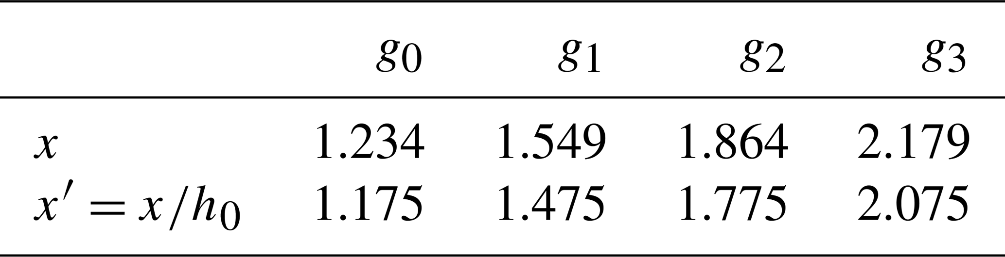
This benchmark problem is based on the 2D laboratory experiments of Grilli and Watts (2005), which were performed at the University of Rhode Island. Refer to the above-mentioned work to get a detailed description of the present benchmark. Figure 3 depicts the sketch of the laboratory experiment design. The 2D slide model is semi-elliptical, lead-loaded, and rolling down a smooth slope with a slope angle (2 mm above the slope), in between two vertical side walls, 20 cm apart. The water depth is h0 = 1.05 m over the flat bottom part. The slide dimensions were length B = 1 m, maximum thickness T=Tref = 0.052 m, and width w = 0.2 m. The model initial submergence d was varied in experiments and the free-surface elevation recorded at four capacitance wave gauges installed at locations: x′ = 1.175, 1.475, 1.775, and 2.075 m, with the first location being nearly identical to = 1.168 m (where the tilde variables, such as x′, mean than non-dimensional units are used – see Table3).
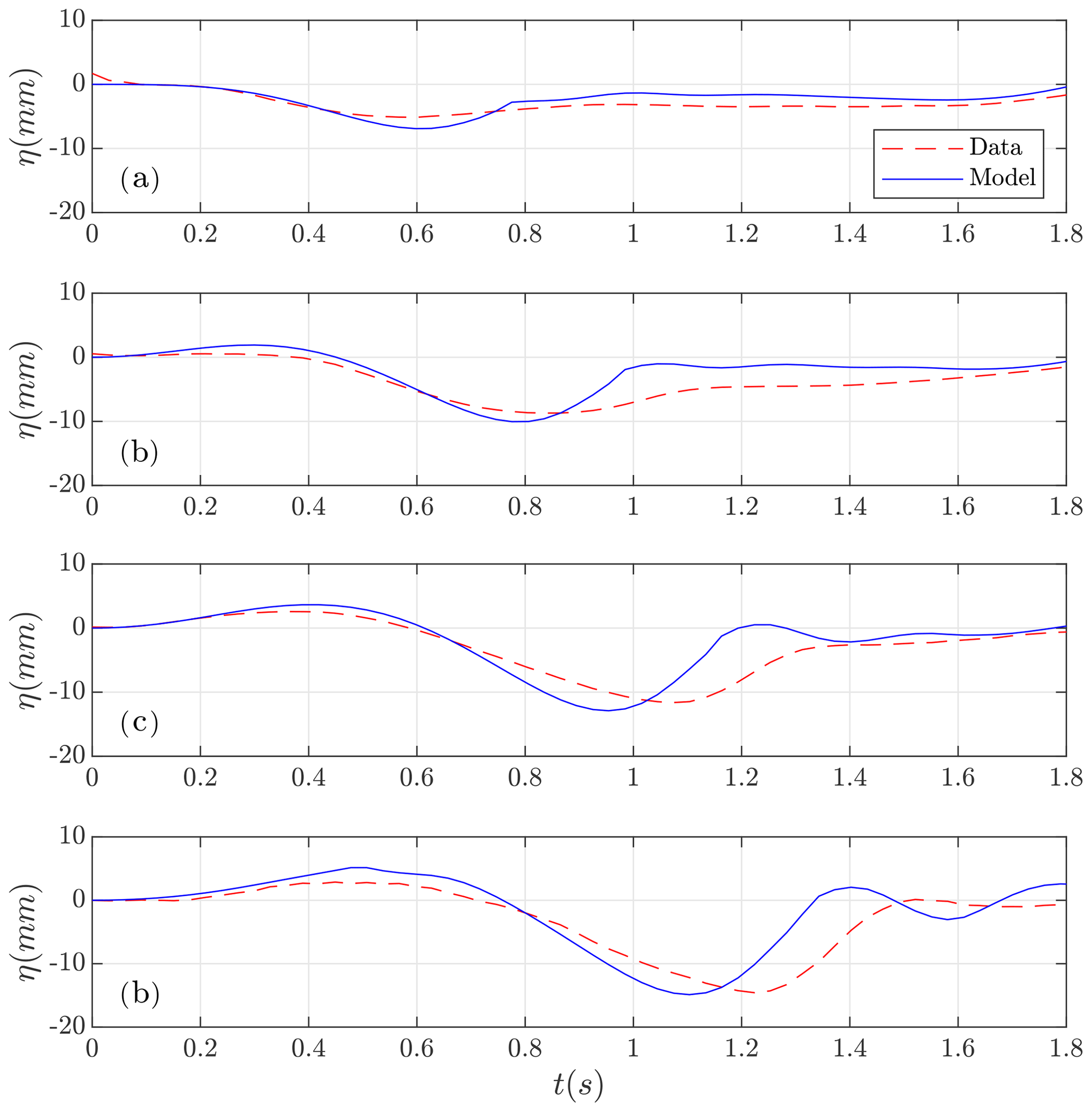
Figure 5BP1. Filtered data (in red) and numerically simulated (in blue) time series at wave gauges (a) g0, (b) g1, (c) g2, and (d) g3.
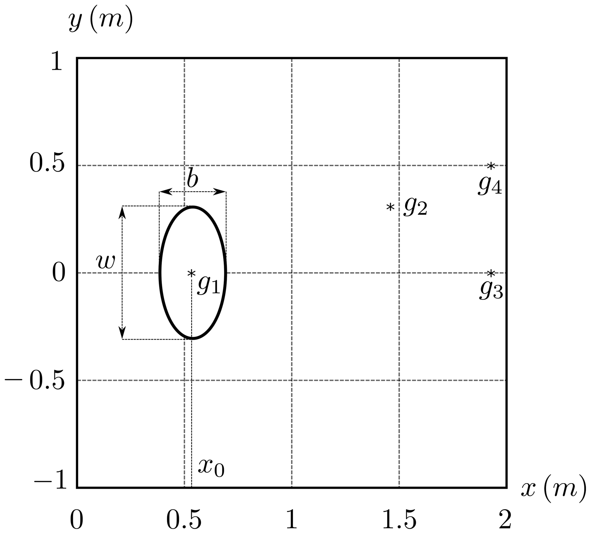
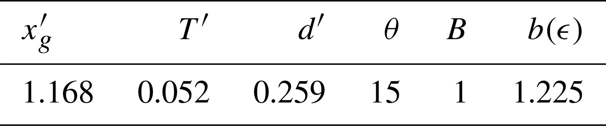
Table 3Gauge positions in dimensional and non-dimensional units.
In this benchmark, two items remained not completely determined in the original description provided: the first one is related with the initialization of the numerical experiment, and the second one is related with how and where the solid moving block must stop. Other small issues related to the description of the benchmark were put forward in Macías et al. (2017) in our NTHMP report.
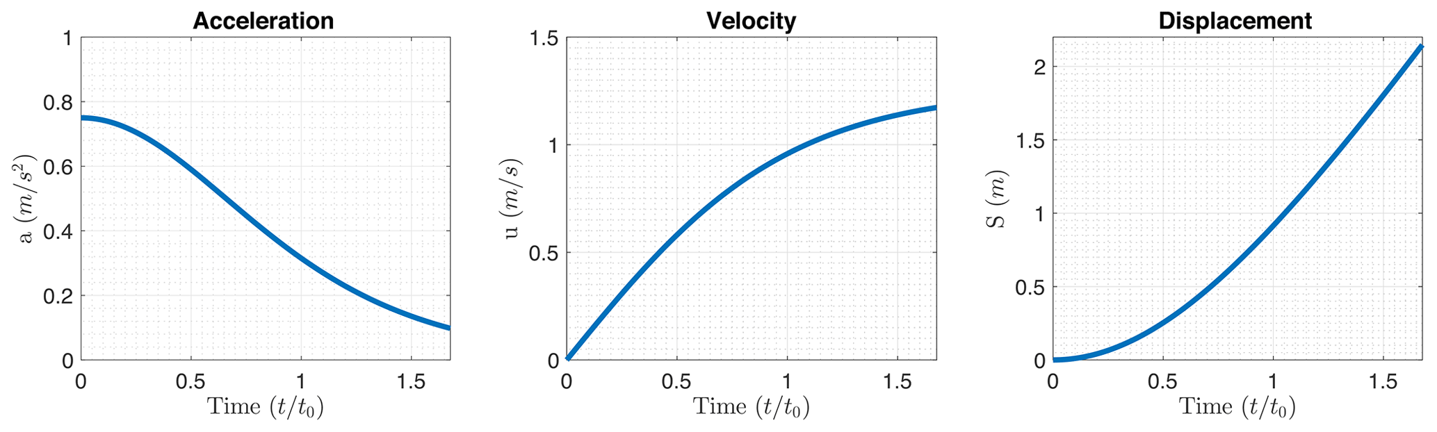
The motion of the rigid slide was prescribed as a function of time as
where m, s, a0=0.75 m/s2, and ut=1.258 m/s is the terminal velocity. Figure 4 shows the prescribed acceleration, velocity, and rigid slide displacement. In the laboratory experiment, the block is stopped at time s, and we replicate this behavior in the numerical model. We also performed numerical experiments (not presented here) where the block continued moving at constant speed.
The benchmark here consists of using the above information on slide shape, submergence, and kinematics, together with reproducing the experimental setup to simulate surface elevations measured at the four wave gauges (average of two replicates of experiments provided).
Then, in order to reproduce the lab experiment, the interval discretized with Δx=0.02 m is the computational domain considered. In the vertical, taking three layers seems to produce optimal results. Increasing the number of layers gives similar results, increasing the computational cost. The stability CFL number was set to 0.9 and g=9.81. The numerical simulation performed was 4 s long in real time. As boundary conditions, outflow conditions were imposed at
In Fig. 5 the comparison of the numerical results with the filtered lab-measured data is presented. A good overall agreement between them can be observed. Some discrepancies can be seen after drawdown in all the gauges. This behavior could also be observed, except for the last gauge, in Grilli and Watts (2005) results. These authors explained that this behavior could be due to unwanted surface tension effects. Given this comparison, and considering the experimental variations and errors inherent to laboratory work and data processing, it can be concluded that the Multilayer-HySEA model optimally performs the present benchmark test.
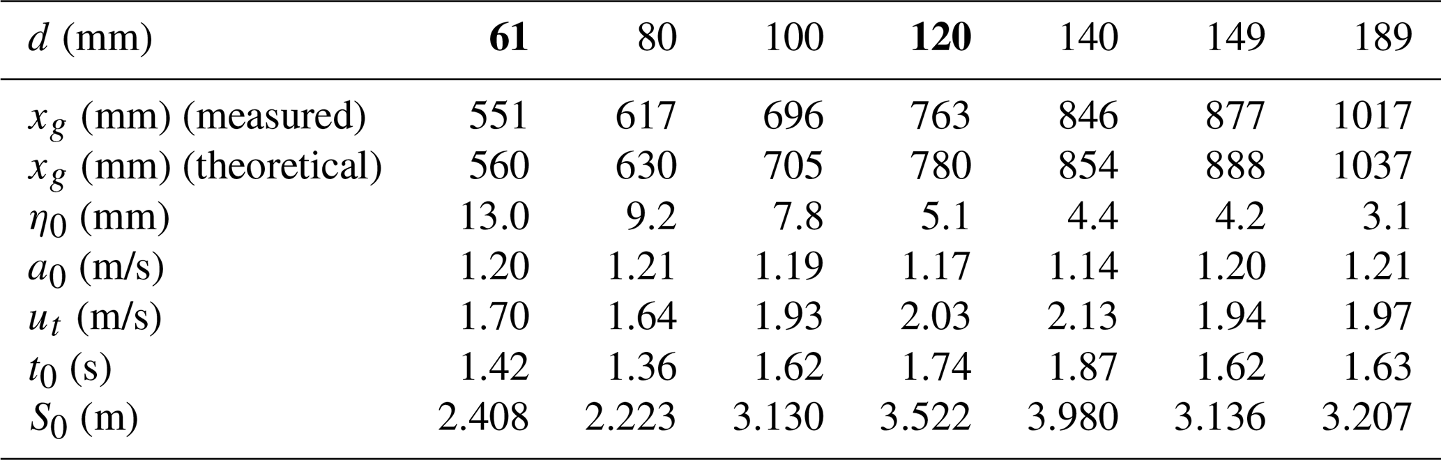
Table 4Measured and curve-fitted slide and wave parameters for the seven experiments performed by Enet and Grilli (2007). Measured characteristic amplitude: η0 (at x=x0). Slide kinematics parameters: a0,ut, and t0. The experiments marked in bold correspond to the two cases proposed by the NTHMP and used as main references in the present work (see text).
5.2 Benchmark problem 2: three-dimensional submarine solid block
This second benchmark consists of a 3D extension of BP1. The longitudinal sketch of the experiment is the same as in Fig. 3. In the horizontal plane, cross sections are elliptic, and the plan view of the rigid slide, for the case d=61 mm, is presented in Fig. 6. It is based on the 3D laboratory experiments of Enet and Grilli (2007). The experiments were also performed at the University of Rhode Island in a water wave tank of width 3.6 m and length 30 m, with a still-water depth of 1.5 m over the flat bottom portion. As in the previous benchmark, the angle of the plane slope where the slide slid down is θ=15∘. The submarine slide model was built as a streamline Gaussian-shaped aluminum body with an elliptical footprint (see Fig. 6), with down-slope length b=0.395 m, cross-slope width w=0.680 m, and maximum thickness T=0.082 m. Complete details about the analytic definition of the slide shape and the experimental setting can be found in Kirby et al. (2018) and in LTMBW (2017).
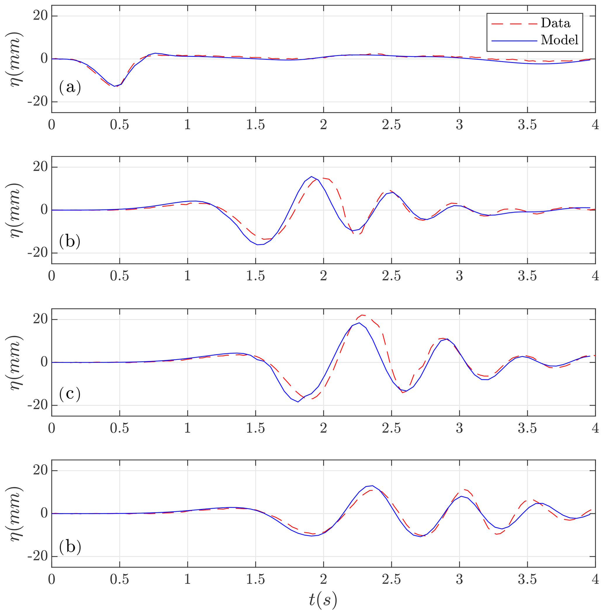
Figure 7Test case d=61 mm. Numerically computed (in blue) time series at wave gauges (a) g1, (b) g2, (c) g3, and (d) g4 compared with the lab-measured data (in red).
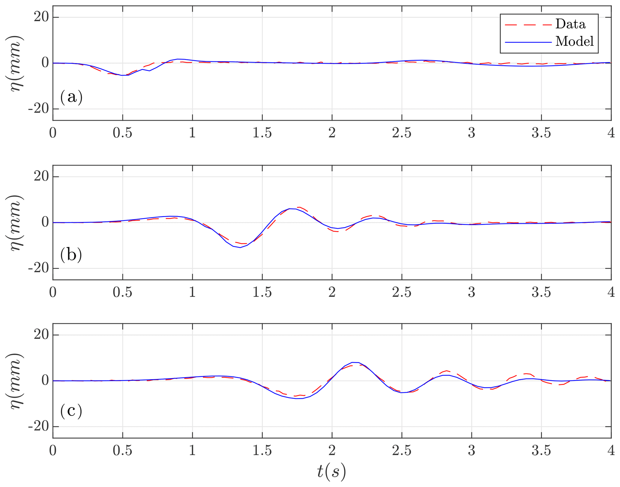
Figure 8Test case d=120 mm. Numerically computed (in blue) time series at wave gauges (a) g1, (b) g2, and (c) g4 compared with the lab-measured data (in red).
For the numerical simulations, the two-dimensional computational domain is considered and discretized with . The number of layers was set to 3. Numerical tests were performed using more layers, and similar results were obtained. The CFL number was set to 0.9 and g=9.81. The simulated time was 6 s. As boundary conditions, rigid wall conditions were imposed at and outflow conditions at .
The benchmark test proposed consists in reproducing the slide shape and complete experimental setup in and using the information about submergence and kinematics to replicate numerically Enet and Grilli's experiments for d=61 and d=120 mm. It is required to simulate surface elevations measured at the four wave gauges (average of two replicates of experiments) and present comparisons of the model with the experimental results.
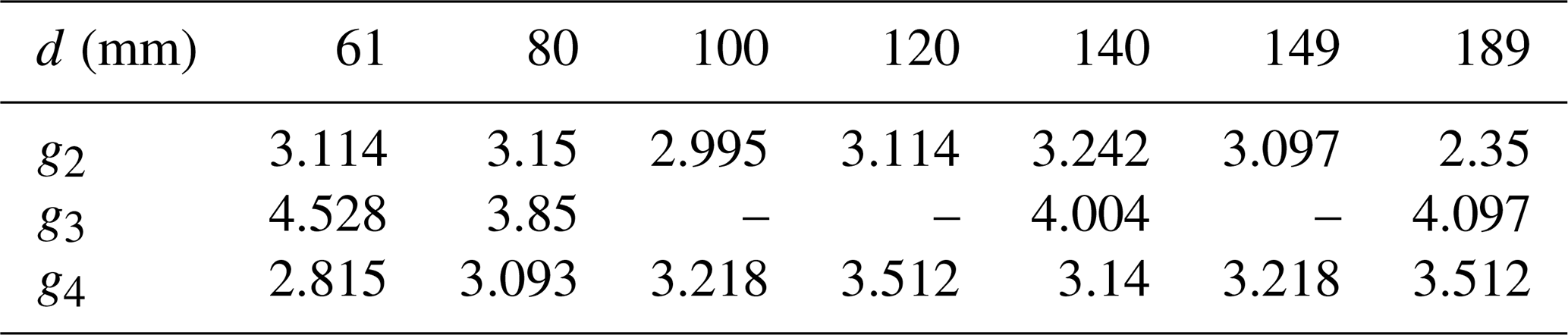
Enet and Grilli (2007) performed experiments for seven initial submergence depths d. They are listed in Table 4, together with values of related slide parameters and some measured tsunami wave characteristics. Here, the numerical results corresponding to the two NTHMP required experiments (for d=61 and d=120 mm) will be presented first, then, as data for the seven experiments are provided, the comparison for the remaining five cases will also be presented.
Table 5Wave gauge locations (x,y) in millimeters, as shown in Fig. 6.
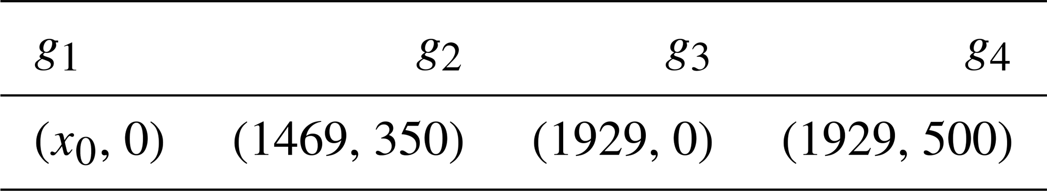
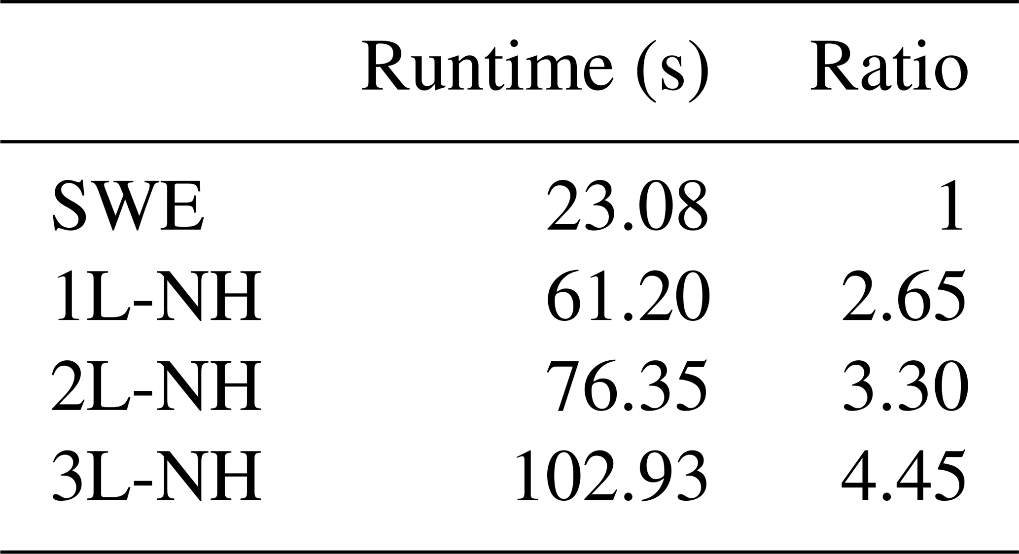
Table 6Execution times in seconds for SWE and non-hydrostatic GPU implementations. Ratios compared with SWE.
In Fig. 7 the comparison of the Multilayer-HySEA model numerical results with measured data for the first case, d=61 mm, in the four gauges is presented. An excellent agreement can be observed between these time series. The comparisons for the second required case (d=120 mm) in the three gauges with data provided (gauge g3 was not available) are shown in Fig. 8. Good agreement can also be observed in this case. Finally, Fig. 9 shows the comparison for the five remaining cases provided by Enet and Grilli. In all cases (for all submergences), a good agreement between simulated results and measured lab data can be observed.
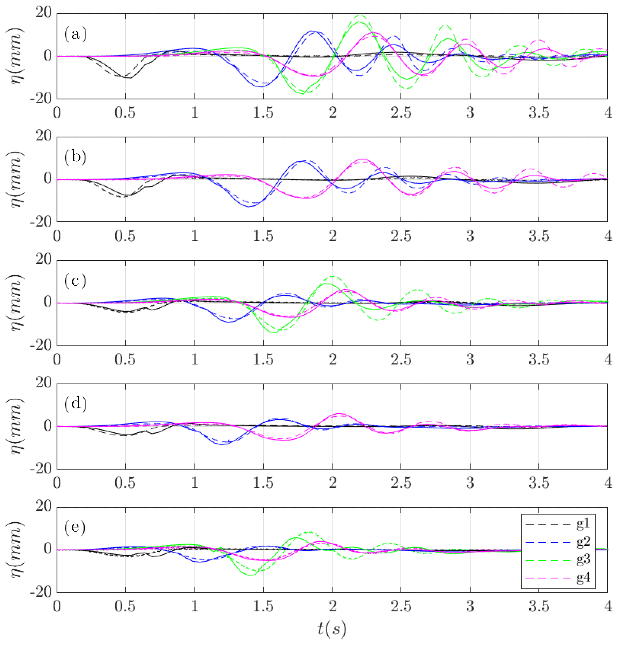
Figure 9Comparison of data and numerical solution time series at wave gauges (dashed) for the cases (a) d=80 mm, (b) d=100 mm, (c) d=140 mm, (d) d=149 mm, and (e) d=189 mm.
In Table 6, the execution times for simulations performed on an NVIDIA Tesla P100 GPU are presented. It can be observed that including non-hydrostatic terms in the non-linear shallow water equations results in an increase in the computational time of 2.65 times. If a richer vertical structure is considered, then larger computational times are required. As in the examples for the two and three-layer systems, there is a 3.3 and 4.45 times increase in the computational effort.
Figure 10 shows the comparison, for the four models considered, of the numerical results obtained with the measured data at gauge g4 for the case d=189 mm. It can be observed that a model vertical structure considering only one layer is not enough to reproduce the observed data and that considering two and three layers in the model produces much better numerical results.
Moreover, Table 7 shows the time periods, T, of the time series data in Figs. 7, 8, and 9 for all the wave gauges. To obtain the values for the periods, we have computed the elapsed time between the first two wave troughs in each time series. We have omitted the measurement for wave gauge g1 because it was not clear how to measure the period in this case. Once the period from each time series was measured, we computed the wave number from the dispersion relation given from the Airy theory:
Table 8 shows the computed values kH by solving the dispersion relation (23). On the view of the computed kH values it can be stated that
Since multilayer models have good dispersion relation errors within this range of kH (see Table 1 and Fig. 2), this explains the aforementioned excellent agreement between the computed time series and the measured lab data.
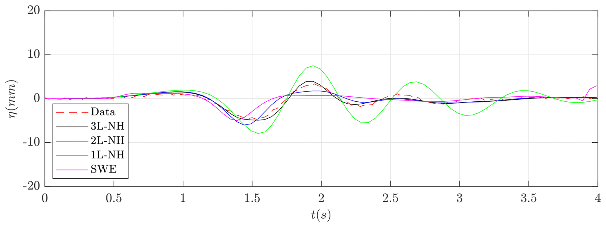
Figure 10Test case d=189 mm. Lab-measured data (red) and numerically computed time series at wave gauge g4 using different numerical models.
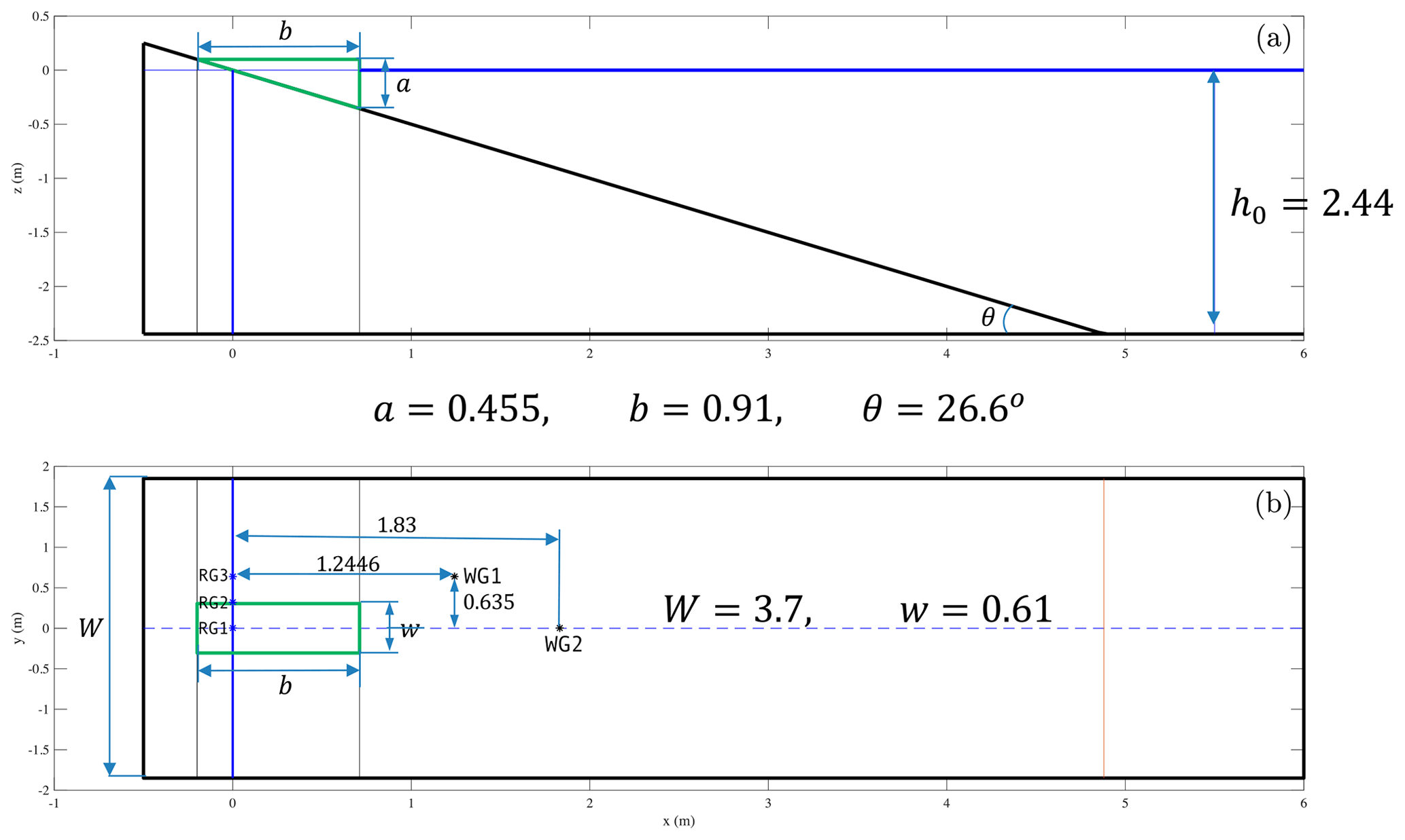
Figure 11Definition sketch for BP3 laboratory experiments – here for a submerged (Δ<0) slide. The upper panel shows the vertical cross section; the lower panel shows the plan view. All units are in meters.
Finally, although the phase velocity for the one-layer system shows an error bounded by only 3.02 % for (see Table 1), it can be seen in Fig. 10 that the one-layer non-hydrostatic pressure system cannot represent the waves correctly. In contrast, the one-layer system tends to amplify waves. This behavior can be explained by observing the shoaling gradient for this model (see Fig. 2). The shoaling gradient verifies the ODE:
where A denotes the amplitude. Thus, it can be stated by inspecting the solutions of the ODE (24) that if the shoaling gradient of the model γ(kH) is underestimated with respect to the Airy theory (γ<γAiry), then in this case the solutions of the system tend to amplify waves for offshore wave propagation. The poor behavior shown by the one-layer system in some cases justifies the need to incorporate the improved multilayer model considered here.
Table 7Measured wave period T(s) for test cases d=61 and 120 (Figs. 7 and 8) and , and 189 (Fig. 9).
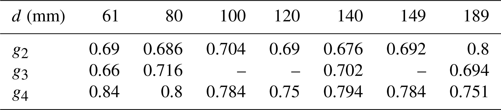
Table 8Computed kH values from the measured wave period (see Table 7) and the Airy dispersion relation for test cases , and 189.
5.3 Benchmark problem 3: three-dimensional submarine/subaerial triangular solid block
This benchmark problem is based on the 3D laboratory experiment of Wu (2004) and Liu et al. (2005) for a series of triangular blocks of several aspect ratios moving down a plane slope into the water from a dry (subaerial) or wet (submarine) location. Figure 11 shows the schematic description of the setup for this benchmark in the case of a partially submerged block. Further details can be found in Kirby et al. (2018) and in LTMBW (2017). The laboratory experiments were conducted in a wave tank at Oregon State University of length 104 m, width 3.7 m, and depth 4.6 m.
A plane slope 1:2 (as the one shown in Fig. 11, upper panel) with was located near one end of the tank and a dissipating beach in the other. In all the experiments, the water depth was h0=2.44 m. The experiments retained for the present benchmark were all performed with a triangular block of length b=0.91 m, width w=0.61 m, and vertical front face m.
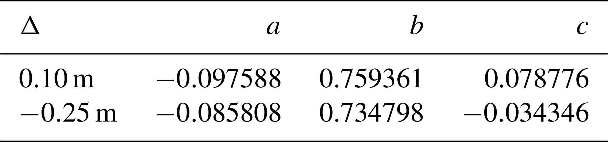
The block movement was provided by means of a polynomial fitting to measured data, giving the horizontal distance as
with and . The polynomial coefficients for the two cases proposed are given in Table 9.
For each case, measured free-surface elevations are given for two wave gauges placed at (in m) and , where x is the distance to the initial coastline and y is the distance to the central cross section (see location in Fig. 11, lower panel). Also measured run-up for each case is given at run-up gauges 2 and 3 in Fig. 11, lower panel, lying on the slope at a distance 0.305 and 0.611 m from the central cross section, respectively.
The two-dimensional computational domain is discretized with and the number of layers was set up to 3. Numerical experiments using a higher number of layers were performed, obtaining similar results. The stability CFL number was set to 0.9 and g=9.81. The simulated time was 4 s. The same boundary conditions, as in the previous case, were imposed.
The numerical results obtained for the subaerial test case are presented in Figs. 12 and 13. Figure 12 depicts the comparison for the time series at the wave gauges and Fig. 13 at the run-up gauges. The same comparison has been performed for the submerged test case, and it is presented in Figs. 14 and 15. The agreement for the wave gauges is quite good for WG1 in both cases. For WG2, just in front of the block, an overshoot after the first depression wave is observed in both cases. This feature is related to the turbulent nature of the experiment. Note that although a turbulent model is not considered here, we have noted that the breaking criteria helps to dissipate energy associated with this turbulent process. For the run-up, the qualitative agreement is quite good, with the larger discrepancies in RG3 for the submarine test case.

Figure 12Subaerial test case. Lab-measured water height (red) and numerical time series (blue) at wave gauges (a) WG1 and (b) WG2.
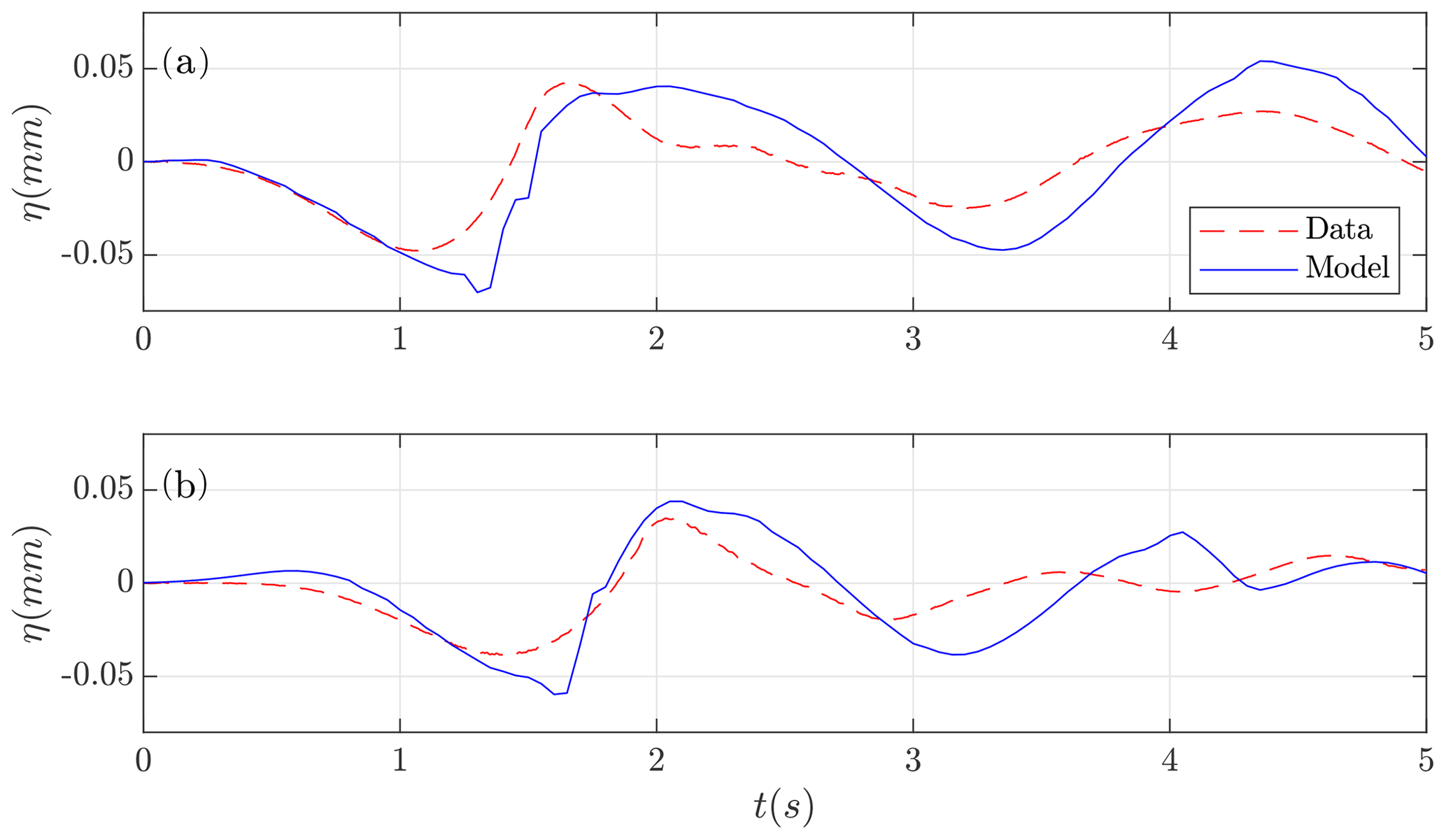
Figure 13Subaerial test case. Lab-measured run-up (red) and numerical time series (blue) at run-up gauges (a) RG2 and (b) RG3.

Figure 14Submerged test case. Lab-measured water height (red) and numerical time series (blue) at wave gauges (a) WG1 and (b) WG2.

Figure 15Submerged test case. Lab-measured run-up (red) and numerical time series (blue) at run-up gauges (a) RG2 and (b) RG3.
Validation of numerical models is a first unavoidable step before their use as predictive tools. This requirement is even more necessary when the developed models are going to be used for risk assessment in natural events where human lives are involved. The present work is the first step in this task for the Multilayer-HySEA model, a novel dispersive multilayer model of the HySEA suite developed at the University of Malaga. This model considers a stratified vertical structure and includes non-hydrostatic terms; this is done in order to include the dispersive effects in the propagation of the waves in a homogeneous, inviscid, and incompressible fluid. The numerical scheme implemented combines a highly robust and efficient finite-volume path-conservative scheme for the underlying hyperbolic system and finite differences for the discretization of the non-hydrostatic terms. In order to increase numerical efficiency, the numerical model is implemented to run in GPU architectures – in particular in NVIDIA graphics cards and using CUDA language. In the case of the traditional SW non-dispersive model, this kind of implementation produces an extremely efficient and fast code (Macías et al., 2020c). Increasing the number of layers in SW models provides an enhanced vertical resolution and, at the same time, increases the computational cost. Despite this, from a computational point of view, the two-layer non-hydrostatic code presents a good computational efficiency, and computing times with respect to the one-layer SWE GPU code are absolutely reasonable, being only from 2 to 2.5 larger than for the one-layer case. In the numerical simulations performed in the present work, the non-hydrostatic wall-clock times are always below 4.45 times those for the traditional SWE HySEA model, for a number of vertical layers up to three. The numerical scheme presented here and the corresponding multilayer SW water model proposed is highly efficient and is able to model dispersive effects with a low computational cost.
Regarding model results, they show a good agreement with the experimental data for the three benchmark problems studied in the present work. In particular, for BP2, but this also occurs for the other two benchmark problems, we have shown that a one-layer, hydrostatic or non-hydrostatic, model is not able to reproduce the complexity in the observed lab data considered in the proposed benchmarks. The waves to be modeled in the test cases proposed here are high in frequency and dispersive. Hence, it is at least necessary that a two-layer structure and non-hydrostatic terms in the model be used in order to capture the dynamics of the generated waves. As noted in Kirby et al. (2018) and in view of the results presented here, the non-hydrostatic multilayer model discussed in this work can adequately represent the physics and behavior of the waves generated at a reasonable low computational cost.
The numerical code used to perform the numerical simulations in this paper is available at the HySEA codes web page at https://edanya.uma.es/hysea/index.php/download (Macías, 2021).
All the data used in the present work and necessary to reproduce the setup of the numerical experiments as well as the laboratory-measured data to compare with can be downloaded from LTMBW (2017) at the web site http://www1.udel.edu/kirby/landslide/. Finally, the NetCDF files containing the numerical results obtained with the Multilayer-HySEA code can be found and downloaded from https://doi.org/10.17632/xtfzrbvcb2.3 (Macías et al., 2020b).
JM led the HySEA codes benchmarking effort undertaken by the EDANYA group, wrote most of the paper, reviewed and edited it, and assisted in the numerical experiments and in their setup. CE implemented the numerical code and performed all the numerical experiments; he also contributed to writing the manuscript. JM and CE did all the figures. MC significantly contributed to the design and implementation of the numerical code.
The authors declare that they have no conflict of interest.
The authors are indebted to Diego Arcas (PMEL/NOAA) and Victor Huérfano (PRSN) for supporting our participation in the 2017 Galveston workshop and to the MMS of the NTHMP for kindly inviting us to that event.
This research has been supported by the Spanish Government–FEDER (MEGAFLOW project, grant no. RTI2018-096064-B-C21) and the Junta de Andalucía–FEDER (grant no. UMA18-Federja-161).
This paper was edited by Maria Ana Baptista and reviewed by two anonymous referees.
Adsuara, J., Cordero-Carrión, I., Cerdá-Durán, P., and Aloy, M.: Scheduled relaxation Jacobi method: Improvements and applications, J. Comput. Phys., 321, 369–413, 2016. a
Ataie-Ashtiani, B. and Najafi-Jilani, A.: Laboratory investigations on impulsive waves caused by underwater landslide, Coast. Eng., 55, 989–1004, https://doi.org/10.1016/j.coastaleng.2008.03.003, 2008. a
Bai, Y. and Cheung, K. F.: Linear shoaling of free–surface waves in multi–layer non–hydrostatic models, Ocean Model., 121, 90–104, https://doi.org/10.1016/j.ocemod.2017.11.005, 2018. a
Castro, M. and Fernández-Nieto, E.: A class of computationally fast first order finite volume solvers: PVM methods, SIAM J. Sci. Comput., 34, A2173–A2196, https://doi.org/10.1137/100795280, 2012. a
Castro, M., Ferreiro, A., García, J., González, J., Macías, J., Parés, C., and Vázquez-Cendón, M.: The numerical treatment of wet/dry fronts in shallow flows: Applications to one-layer and two-layer systems, Math. Comput. Model., 42, 419–439, 2005. a, b
Castro, M., Ortega, S., de la Asunción, M., Mantas, J., and Gallardo, J.: GPU computing for shallow water flow simulation based on finite volume schemes, C. R. Mécanique, 339, 165–184, 2011. a
Chorin, A. J.: Numerical solution of the Navier-Stokes equations, Math. Comput., 22, 745–762, https://doi.org/10.2307/2004575, 1968. a
Cui, H., Pietrzak, J., and Stelling, G.: Optimal dispersion with minimized Poisson equations for non–hydrostatic free surface flows, Ocean Model., 81, 1–12, https://doi.org/10.1016/j.ocemod.2014.06.004, 2014. a
de la Asunción, M., Castro, M., González-Vida, J., Macías, J., Ortega, S., and Sánchez-Linares, C.: East Coast Non-Seismic Tsunamis: A first landslide approach, Tech. Rep., NOAA report, https://doi.org/10.13140/2.1.4645.1520, Universidad de Málaga, Málaga, 9 pp., 2013. a
Enet, F. and Grilli, S.: Experimental study of tsunami generation by three-dimensional rigid underwater landslides, J. Waterw. Port. Coast., 133, 442–454, https://doi.org/10.1061/(ASCE)0733-950X(2007)133:6(442), 2007. a, b, c, d, e
Escalante, C., Fernández-Nieto, E., Morales, T., and Castro, M.: An efficient two–layer non–hydrostatic approach for dispersive water waves, J. Sci. Comput., 79, 273–320, https://doi.org/10.1007/s10915-018-0849-9, 2018a. a, b, c, d, e, f, g, h, i, j, k
Escalante, C., Morales, T., and Castro, M.: Non-hydrostatic pressure shallow flows: GPU implementation using finite volume and finite difference scheme, Appl. Math. Comput., 338, 631–659, https://doi.org/10.1016/j.amc.2018.06.035, 2018b. a, b, c, d, e, f
Escalante, C., Dumbser, M., and Castro, M. J.: An efficient hyperbolic relaxation system for dispersive non-hydrostatic water waves and its solution with high order discontinuous Galerkin schemes, J. Comput. Phys., 394, 385–416, https://doi.org/10.1016/j.jcp.2019.05.035, 2019. a
Fernández, E., Bouchut, F., Bresh, D., Castro, M., and Mangeney, A.: A new Savage-Hutter type model for submarine avalanches and generated tsunami, J. Comp. Phys., 227, 7720–7754, 2008. a, b
Fernández-Nieto, E., Parisot, M., Penel, Y., and Sainte-Marie, J.: A hierarchy of dispersive layer-averaged approximations of Euler equations for free surface flows, Commun. Math. Sci., 16, 1169–1202, 2018. a, b, c, d, e
Fritz, D., Hager, W., and Minor, H.-E.: Lituya Bay case: rockslide impact and wave runup, Science of Tsunami Hazards, 19, 3–22, 2001. a
González-Vida, J. M., Macías, J., Castro, M. J., Sánchez-Linares, C., de la Asunción, M., Ortega-Acosta, S., and Arcas, D.: The Lituya Bay landslide-generated mega-tsunami – numerical simulation and sensitivity analysis, Nat. Hazards Earth Syst. Sci., 19, 369–388, https://doi.org/10.5194/nhess-19-369-2019, 2019. a
Grilli, S. and Watts, P.: Modeling of waves generated by a moving submerged body, Applications to underwater landslides, Eng. Anal. Bound. Elem., 23, 645–656, https://doi.org/10.1016/S0955-7997(99)00021-1, 1999. a
Grilli, S. and Watts, P.: Tsunami Generation by Submarine Mass Failure, I: Modeling, Experimental Validation, and Sensitivity Analyses, J. Waterw. Port. Coast., 131, 283–297, https://doi.org/10.1061/(ASCE)0733-950X(2005)131:6(283), 2005. a, b, c, d
Grilli, S., Vogelmann, S., and Watts, P.: Development of a 3D numerical wave tank for modeling tsunami generation by underwater landslides, Eng. Anal. Bound. Elem., 26, 301–313, https://doi.org/10.1016/S0955-7997(01)00113-8, 2002. a
Heller, V. and Hager, W.: Waves types of landslide generated impulse waves, Ocean Eng., 38, 630–640, 2011. a
Horrillo, J., Grilli, S., Nicolsky, D., Roeber, V., and Zhang, J.: Performance Benchmarking Tsunami Models for NTHMP's Inundation Mapping Activities, Pure Appl. Geophys., 172, 869–884, https://doi.org/10.1007/s00024-014-0891-y, 2015. a
Iglesias, O.: Generación y propagación de tsunamis en el mar Catalano-Balear, PhD thesis, Universitat de Barcelona, Barcelona, Spain, available at: http://hdl.handle.net/2445/68704 (last access: 20 February 2021), 2015. a
Kazolea, M. and Delis, A. I.: A well-balanced shock-capturing hybrid finite volume-finite difference numerical scheme for extended 1D Boussinesq models, Appl. Numer. Math., 67, 167–186, https://doi.org/10.1016/j.apnum.2011.07.003, 2013. a
Kirby, J., Grilli, S., Zhang, C., Horrillo, J., Nicolsky, D., and Liu, P. L.-F.: The NTHMP Landslide Tsunami Benchmark Workshop, Galveston, Texas, USA, 9–11 January 2017, Tech. Rep., Research Report CACR-18-01, 2018. a, b, c, d, e, f, g
Kurganov, A. and Petrova, G.: A second-order well-balanced positivity preserving central-upwind scheme for the Saint-Venant system, Commun. Math. Sci., 5, 133–160, 2007. a, b
Liu, P. L.-F., Wu, T.-R., Raichlen, F., Synolakis, C. E., and Borrero, J. C.: Runup and rundown generated by three-dimensional sliding masses, J. Fluid Mech., 536, 107–144, https://doi.org/10.1017/S0022112005004799, 2005. a, b, c
Liu, P. L.-F., Yeh, H., and Synolakis, C.: Advanced Numerical Models for Simulating Tsunami Waves and Runup, World Scientific, 10, 344 pp., https://doi.org/10.1142/6226, 2008. a
LTMBW: Landslide Tsunami Model Benchmarking Workshop, Galveston, Texas, USA, 9–11 January 2017, available at: http://www1.udel.edu/kirby/landslide/index.html (last access: 25 April 2020), 2017. a, b, c, d
Lynett, P. and Liu, P. L.-F.: A numerical study of submarine–landslide–generated waves and run–up, P. Roy. Soc. Lond. A Mat., 458, 2885–2910, https://doi.org/10.1098/rspa.2002.0973, 2002. a
Lynett, P. and Liu, P. L.-F.: A two–layer approach to wave modelling, P. Roy. Soc. Lond. A Mat., 460, 2637–2669, 2004. a, b
Lynett, P., Gately, K., Wilson, R., Montoya, L., Arcas, D., Aytore, B., Bai, Y., Bricker, J., Castro, M., Cheung, K., David, C., Dogan, G., Escalante, C., González-Vida, J., Grilli, S., Heitmann, T., Horrillo, J., Kanouglu, U., Kian, R., Kirby, J., Li, W., Macías, J., Nicolsky, D., Ortega, S., Pampell-Manis, A., Park, Y., Roeber, V., Sharghivand, N., Shelby, M., Shi, F., Tehranirad, B., Tolkova, E., Thio, H., Velioglu, D., Yalciner, A., Yamazaki, Y., Zaytsev, A., and Zhang, Y.: Inter-model analysis of tsunami-induced coastal currents, Ocean Model., 114, 14–32, https://doi.org/10.1016/j.ocemod.2017.04.003, 2017. a
Ma, G., Shi, F., and Kirby, J.: Shock-capturing non-hydrostatic model for fully dispersive surface wave processes, Ocean Model., 43–44, 22–35, 2012. a
Macías, J.: HySEA codes, available at: https://edanya.uma.es/hysea/index.php/download, last access: 20 February 2021. a
Macías, J., Vázquez, J., Fernández-Salas, L., González-Vida, J., Bárcenas, P., Castro, M., del Río, V. D., and Alonso, B.: The Al-Borani submarine landslide and associated tsunami, A modelling approach, Mar. Geol., 361, 79–95, https://doi.org/10.1016/j.margeo.2014.12.006, 2015. a
Macías, J., Castro, M., Ortega, S., Escalante, C., and González-Vida, J.: Performance Benchmarking of Tsunami-HySEA Model for NTHMP's Inundation Mapping Activities, Pure Appl. Geophys., 174, 3147–3183, https://doi.org/10.1007/s00024-017-1583-1, 2017. a
Macías, J., Escalante, C., Castro, M., González-Vida, J., and Ortega, S.: HySEA model, Landslide Benchmarking Results, Tech. Rep., NTHMP report, Universidad de Málaga, Málaga, 28 pp., https://doi.org/10.13140/RG.2.2.27081.60002, 2017. a, b
Macías, J., Escalante, C., and Castro, M.: Performance assessment of Tsunami-HySEA model for NTHMP tsunami currents benchmarking, Laboratory data, Coast. Eng., 158, 103667, https://doi.org/10.1016/j.coastaleng.2020.103667, 2020a. a
Macías, J., Escalante, C., and Castro, M.: Numerical results in Multilayer-HySEA model validation for landslide generated tsunamis, Part I: Rigid slides, Dataset, Mendeley Data, https://doi.org/10.17632/xtfzrbvcb2.3, 2020b. a
Macías, J., Ortega, S., González-Vida, J., and Castro, M.: Performance assessment of Tsunami-HySEA model for NTHMP tsunami currents benchmarking, Field cases, Ocean Model., 152, 101645, https://doi.org/10.1016/j.ocemod.2020.101645, 2020c. a, b
Macías, J., Escalante, C., and Castro, M. J.: Multilayer-HySEA model validation for landslide-generated tsunamis – Part 2: Granular slides, Nat. Hazards Earth Syst. Sci., 21, 791–805, https://doi.org/10.5194/nhess-21-791-2021, 2021. a
Madsen, P. and Sorensen, O.: A new form of the Boussinesq equations with improved linear dispersion characteristics, Part II: A slowing varying bathymetry, Coast. Eng., 18, 183–204, 1992. a
Ricchiuto, M. and Filippini, A. G.: Upwind residual discretization of enhanced Boussinesq equations for wave propagation over complex bathymetries, J. Comput. Phys., 271, 306–341, https://doi.org/10.1016/j.jcp.2013.12.048, 2014. a
Roeber, V., Cheung, K. F., and Kobayashi, M. H.: Shock-capturing Boussinesq-type model for nearshore wave processes, Coast. Eng., 57, 407–423, https://doi.org/10.1016/j.coastaleng.2009.11.007, 2010. a, b, c, d
Sánchez-Linares, C.: Simulación numérica de tsunamis generados por avalanchas submarinas: aplicación al caso de Lituya Bay, Master's thesis, University of Málaga, Spain, 2011. a
Schäffer, H. A. and Madsen, P. A.: Further enhancements of Boussinesq-type equations, Coast. Eng., 26, 1–14, https://doi.org/10.1016/0378-3839(95)00017-2, 1995. a, b, c
ten Brink, U., Chaytor, J., Geist, E., Brothers, D., and Andrews, B.: Assessment of tsunami hazard to the US Atlantic margin, Mar. Geol., 353, 31–54, https://doi.org/10.1016/j.margeo.2014.02.011, 2014. a
Watts, P., Grilli, S. T., Kirby, J. T., Fryer, G. J., and Tappin, D. R.: Landslide tsunami case studies using a Boussinesq model and a fully nonlinear tsunami generation model, Nat. Hazards Earth Syst. Sci., 3, 391–402, https://doi.org/10.5194/nhess-3-391-2003, 2003. a
Watts, P., Grilli, S. T., Tappin, D. R., and Fryer, G. J.: Tsunami Generation by Submarine Mass Failure, II: Predictive Equations and Case Studies, J. Waterw. Port. Coast., 131, 298–310, https://doi.org/10.1061/(ASCE)0733-950X(2005)131:6(298), 2005. a
Wu, T.-R.: A numerical study of three-dimensional breaking waves and turbulence effects, PhD thesis, Cornell University, New York, 283 pp., 2004. a, b, c
https://edanya.uma.es/hysea (last access: 18 February 2021).