the Creative Commons Attribution 4.0 License.
the Creative Commons Attribution 4.0 License.
 | 11 Feb 2021
Predicting power outages caused by extratropical storms
Ilona Láng
Alexander Jung
Antti Mäkelä
Strong winds induced by extratropical storms cause a large number of power outages, especially in highly forested countries such as Finland. Thus, predicting the impact of the storms is one of the key challenges for power grid operators. This article introduces a novel method to predict the storm severity for the power grid employing ERA5 reanalysis data combined with forest inventory. We start by identifying storm objects from wind gust and pressure fields by using contour lines of 15 m s−1 and 1000 hPa, respectively. The storm objects are then tracked and characterized with features derived from surface weather parameters and forest vegetation information. Finally, objects are classified with a supervised machine-learning method based on how much damage to the power grid they are expected to cause. Random forest classifiers, support vector classifiers, naïve Bayes processes, Gaussian processes, and multilayer perceptrons were evaluated for the classification task, with support vector classifiers providing the best results.
- Article
(2808 KB) - Full-text XML
- Companion paper
- BibTeX
- EndNote


Strong winds caused by extratropical storms are among the most significant natural hazards in Europe, causing massive damage to the forests and society (e.g., Schelhaas et al., 2003; Schelhaas, 2008; Ulbrich et al., 2008; Seidl et al., 2014; Valta et al., 2019); extratropical storms are responsible for 53 % of all losses related to natural hazards in Europe (Kron and Schuck, 2013). Such storms pose a huge challenge for power distribution companies in highly forested countries such as Finland (Gardiner et al., 2010) where falling trees cause power outages for hundreds of thousands of customers every year (Niemelä, 2018). The windstorms create a significant risk for the power supply in Finland, which has over 90 000 km of overhead lines (70 % are part of the medium-voltage, 1–35 kV, network) passing through forest (Kufeoglu and Lehtonen, 2015). Between the years 2010 and 2018, on average 46 % of all transmission faults in Finland were caused by extratropical storms (Finnish Energy, 2010–2018). During the years of the most damaging storms, 2011 and 2013, the share of windstorm damage of all fault causes was up to 69 % (Finnish Energy, 2011, 2013). The need for managing power interruptions is even more urgent since the power suppliers in Finland are obliged to financially compensate customers of urban areas after 6 h and rural areas after 36 h of interruption in electricity distribution (Nurmi et al., 2019). Thus they require a large workforce to fix caused damage rapidly.
As Ulbrich et al. (2009) describe, there is no scientific consensus on how the occurrence and magnitude of extratropical storms will evolve in the future. Based on existing literature, the windstorm-related damage are increasing, while it remains unclear whether this is due to the higher exposure of society or the number and intensity of extratropical storms. Gregow et al. (2017) discovered that windstorm damage had increased significantly during the previous 3 decades, especially in northern, central, and western Europe. Also, several other studies suggest an increase in wind-related damage in Europe (Csilléry et al., 2017; Haarsma et al., 2013; Gardiner et al., 2010). Interestingly, some studies detected a decrease in the total number of extratropical storms (i.e., Donat et al., 2011), while others found an increase in the number of extreme storms in specific regions, like western Europe and the northeast Atlantic (Pinto et al., 2013). Another supporting view of a potential increase in extratropical storms in northern Europe can be found in the IPCC (2018) report. The report states that extratropical storm tracks are shifting towards the poles, which might affect the storminess in northern Europe. Thus, it may be concluded that the losses related to extratropical storms are also likely to increase, especially in northern Europe. However, as Barredo (2010) emphasizes, the cause for increased losses can at least partly be explained by the increasing exposure of society rather than the increased number of windstorms.
Several previous studies respond to the demand for storm impact estimation for power distribution, many of them focusing on the hurricane-induced power blackouts in northern America (Eskandarpour and Khodaei, 2017; Guikema et al., 2014, 2010; Nateghi et al., 2014; Han et al., 2009; Wang et al., 2017; Allen et al., 2014; Chen and Kezunovic, 2016; He et al., 2017; Liu et al., 2018). Convective thunderstorms have also been investigated thoroughly. Li et al. (2015) introduced an area-based outage prediction method further developed to take power grid topology into account (Singhee and Wang, 2017). Shield (2018) studied outage prediction by applying a random forest classifier to weather forecast data in a regular grid. Kankanala et al. used data from ground observation stations and experimented regression (Kankanala et al., 2011), a multilayer perceptron neural network (Kankanala et al., 2012), and ensemble learning (Kankanala et al., 2014) to predict outages caused by wind and thunder. The Bayesian outage probability (BOP) prediction model developed by Yue et al. (2018) combines weather radar data and unifies it to a regular grid. Cintineo et al. (2014) create spatial objects from satellite and weather radar data, and they track and classify the objects with the naïve Bayesian classifier. Rossi (2015) developed a method to detect and track convective storms. The method was further developed to predict power outages (Tervo et al., 2019).
While much work exists on damage caused by hurricanes and convective thunderstorms, relatively few examples exist relating to outages caused by mid-latitude extratropical storms differing from hurricanes and convective storms in available data, time span, and applicable methods for detecting and tracking. Extratropical storms are considered, for example, in Yang et al. (2020), where different decision tree methods are applied to a regular grid in the outage prediction task. Cerrai et al. (2019) also use decision trees and regular grids for the outage prediction, taking tree-leaf conditions into account as a predictive feature. Related forest damage studies have been conducted with random forest classifiers and neural networks. Hart et al. (2019) showed that random forest regression and artificial neural networks could predict the number of falling trees in France caused by the wind. Hanewinkel (2005) conducted a similar study in Germany using artificial neural networks. Artificial neural networks have been used to predict extreme weather in Finland (Ukkonen et al., 2017; Ukkonen and Mäkelä, 2019). The framework of Masson-Delmotte et al. (2018) emphasizes that the impacts of extreme weather risks can be analyzed by estimating the hazard, vulnerability, and exposure. In an increasing manner, connecting these fields (i.e., the natural hazard with the societal factors) is done with machine learning (Chen et al., 2008).
We present a novel method to identify, track, and classify extratropical storm objects based on how many power outages they are expected to induce. We adapt convective storm object detection (Rossi, 2015; Tervo et al., 2019; Cintineo et al., 2014) to find potentially harmful areas from extratropical storms by contouring objects from pressure and wind gust fields. Instead of highly localized convective storms, we aim at larger but still regional geospatial accuracy so that, for example, damage in western and eastern Finland can be distinguished. We train a supervised machine-learning model to classify storm objects according to their damage potential. To our knowledge, our method is the first that employs the extratropical storm objects as polygons and combines them with meteorological and non-meteorological features to predict power outages. The method can be used as a decision support tool in power distribution companies or as part of elaborating impact forecast by duty forecasters in national hydro-meteorological centers. The ERA5 atmospheric reanalysis (Hersbach et al., 2018) provides the primary meteorological input data for this study, while the national forest inventory provided by The Natural Resources Institute Finland (Luke) is used to represent the forest conditions in the prediction. Finally, historical power outages from two sources are used to train the model. However, the operational use of the model would require the use of weather prediction data instead of reanalysis.
This paper is organized as follows: Sect. 2 presents the used data, which is followed by a step-by-step method description in Sect. 3. Section 3.1 discusses identifying storm objects and explains the storm tracking algorithm. Section 3.2 considers storm and forest characteristics, hereafter called features. Section 3.3 discusses how to define labels of storm objects based on the outage data. Section 3.4 describes the used machine-learning methods. In Sect. 4, we discuss the performance of the method. Finally, Sect. 5 includes a discussion and conclusions.
We base our method on three main data sources: ERA5 reanalysis data (Hersbach et al., 2019), a multi-source national forest inventory (ms-nfi) provided by the Natural Resources Institute Finland (Luke), and occurred power outages obtained from two sources. First, the local dataset is gathered from two power distribution companies, Loiste and Järvi-Suomen Energia (JSE), located in eastern Finland. Second, the national dataset is obtained from Finnish Energy (ET), a branch organization for the industrial and labor market policy of the energy sector. All data consider years from 2010 to 2018.
ERA5 is the newest-generation reanalysis data provided by ECMWF. ERA5 covers the years from 1979 onward with a 1 h temporal resolution, has a horizontal resolution of 31 km, and covers the atmosphere using 137 levels up to a height of 80 km (Hersbach et al., 2019). Compared to in situ wind observations, reanalysis data provide a spatiotemporally wider dataset. However, a question may arise about the accuracy of the reanalysis data. Ramon et al. (2019) examined the wind speed characteristics of a total of five state-of-the-art global reanalyses concerning 77 instrumented towers. In their study, ERA5 had the best agreement with in situ observations on daily timescales; this suggests the ERA5 wind parameters to be adequate in windstorm damage examinations as well. ERA5 data are also known to contain unrealistically large surface wind speeds in some locations (European Centre for Medium-Range Weather Forecasts, 2019). None of these locations are, nevertheless, inside the geographical domain of this work.
The multi-source forest inventory data are based on field measurements, satellite observations, digital maps, and other geo-referenced data sources (Mäkisara et al., 2016). The data consist of estimates for the forest age, tree species dominance, mean and total volume, and biomass (total and tree-species-specific). The original geospatial resolution of the data is 16 m, which has been reduced to approximately 1.6 km resolution to speed up the processing. Taking into account the size of extratropical cyclones (diameter ∼1000 km) and the wide areas where wind damage typically occurs near the cold front, we consider a resolution of 1.6 km to be sufficiently high for modeling windstorm damage.
Power outage data are obtained from two complementary sources. The national dataset is acquired from Finnish Energy (2010–2018), who aggregates the data from power distribution companies in Finland. The national data are provided only for research purposes and for areas containing a minimum of six grid companies; this is, for example, to ensure energy users' anonymity. Therefore, the national dataset does not include exact locations of the faults. We have also obtained some parts of the data with better spatial accuracy from two individual power distribution companies. In this paper, we refer to these data as the local dataset. In the local dataset, the fault locations are reported in relation to transformers; i.e., the spatial resolution of the outages ranges from a few meters to kilometers.
Figure 1 illustrates the geographical coverage of the power outage data. The local dataset contains all outages from 2010 to 2018 in the northern area (Loiste) and outages related to major storms in the southern area (JSE), shown in Fig. 1a. The national dataset contains all outages in Finland from 2010 to 2018 divided into five regions, shown in Fig. 1b. The national dataset contains in total 6 140 434 outages with relatively low geographical accuracy. On the other hand, the local dataset represents a substantially smaller geographical area with a good geographical accuracy but contains only 22 028 outages in total. We train our classification models, described in more detail in Sect. 3.4, with both datasets to evaluate their performance for different types of data.
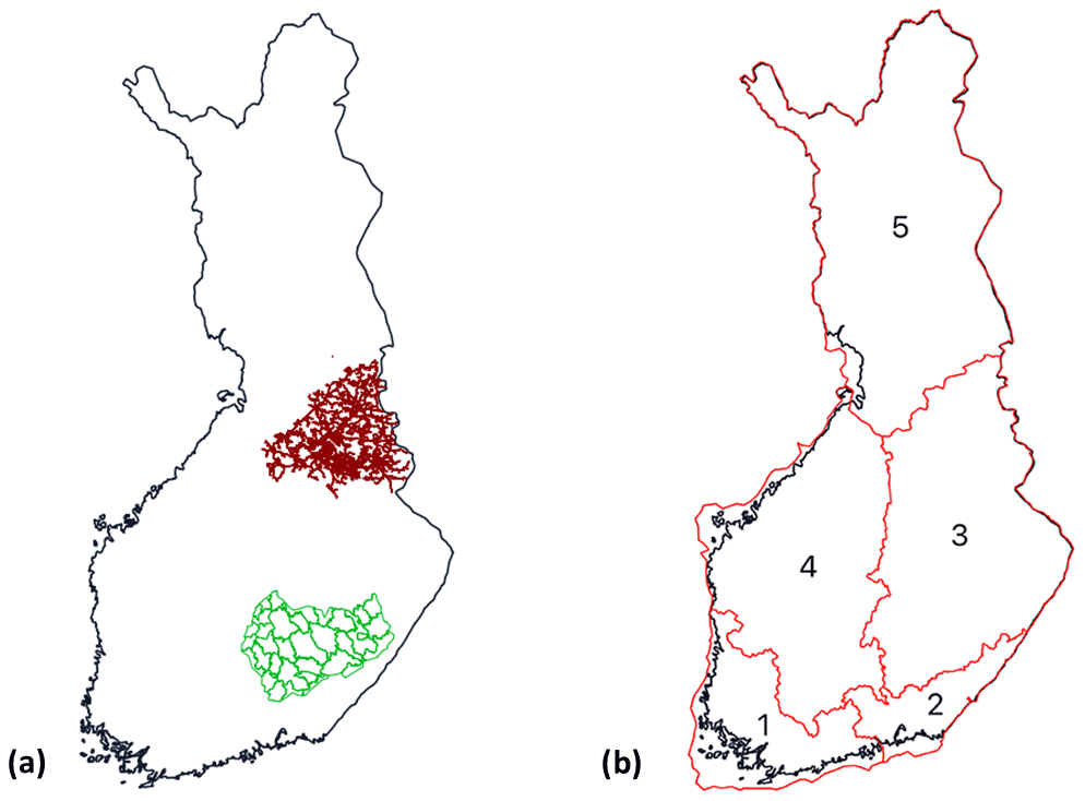
Figure 1(a) Geographical coverage of the outage data (local dataset). The red lines represent the power grid of Loiste (northern grid company) and the green lines the operative areas of JSE (southern grid company). Outages of the local dataset are collected from both areas. (b) Regions in the national outage dataset. Outages are gathered from all of Finland and aggregated to the regions shown in the figure.
We predict power outages by classifying storm objects identified from gridded weather data into three classes based on the number of power outages the storm typically causes. The overall process consists of the following steps: (1) identifying storm objects from weather fields by finding contour lines of particular thresholds, (2) tracking the storm object movement, (3) gathering features of the storm objects, and (4) classifying each storm object individually. The classification is conducted for each storm object separately to distinguish the different damage potential. Tracking is, however, necessary to gather necessary features such as object movement speed and direction. In the following, we discuss these phases in more detail.
3.1 Identifying and tracking storm objects
Storm objects are identified by finding contour lines of 10 m wind gust fields using 15 m s−1 thresholds from the ERA5 surface level grid with a time step of 1 h. The contouring algorithm is capable of finding interior rings of the polygons. The used wind gust fields did not, however, contain such cases. Thus one storm object represents a solid area (polygon) where the hourly maximum wind gust exceeds 15 m s−1 during one particular hour. The threshold of 15 m s−1 is selected as different sources indicate Finland being vulnerable for windstorms and rather moderate winds (from 15 m s−1) causing damage to forests (Valta et al., 2019; Gardiner et al., 2013). Valta et al. (2019) developed a method to estimate the windstorm impacts on forests by combining the recorded forest damage from the nine most intense storms and their observed maximum inland wind gusts. According to the formula developed in the study, the inland wind gusts of 15 m s−1 alone result in forest damage of 1800 m3. We also identify pressure objects by finding contour lines using a 1000 hPa threshold to connect potentially distant storm objects around the low-pressure center to the same storm event.
After identification, storm objects are tracked by connecting them with each other. Each storm object is first connected to nearby pressure objects from the current and preceding time steps. If pressure objects do not exist within the distance threshold, the object is connected to nearby storm objects from the current and preceding time steps. The algorithm enables the assignment of each storm object to an overall event (low-pressure system) and tracking of the objects' movement. Algorithm 1 shows the details of the process.
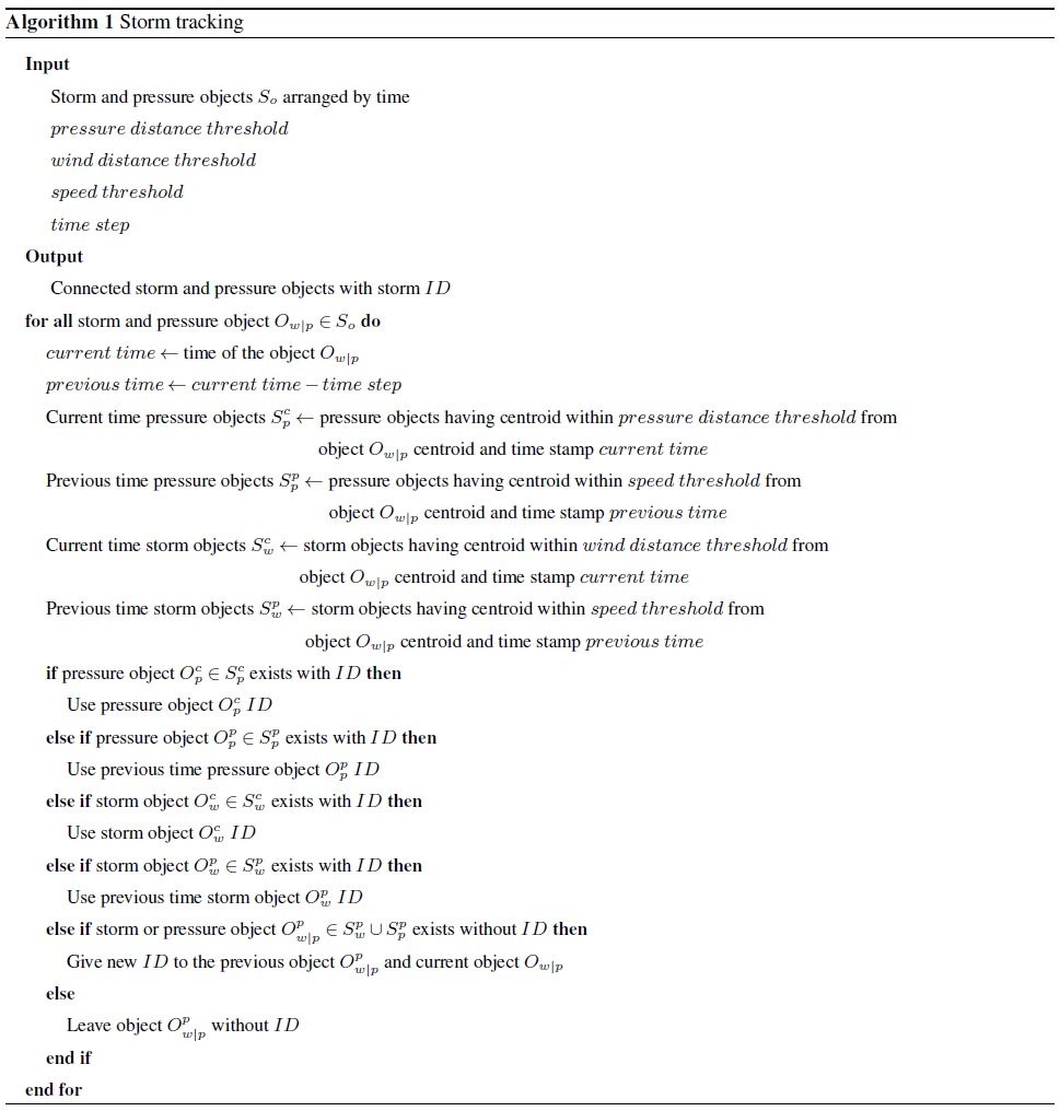
We use a 500 km distance threshold for the distance between the storm and pressure objects. As the typical diameter of an extratropical storm is approximately 1000 km (Govorushko, 2011), we assume the damaging storm objects to situate a maximum 500 km from the center of the low pressure. The threshold for movement speed is 200 km h−1 for storm objects and 45 km h−1 for pressure objects. In other words, storm objects are not assumed to move more than 200 km and pressure objects more than 45 km from the preceding hourly time step (Govorushko, 2011). Convective storms may move faster but are outside the focus of this work.
3.2 Extracting storm object features
We characterize the storm objects identified by the methods discussed in Sect. 3.1 using the features listed in Table 1. The features are structured as four groups. The first group is a number of object characteristics such as size and movement speed and direction, which are calculated from the contoured storm objects themselves. As the second group, relevant weather conditions, such as wind speed, temperature, and others, are extracted from ERA5 data. We aggregate values as a minimum, maximum, average, and standard deviation calculated over all grid cells under the object coverage to represent each parameter with one number. Third, as most of the outages are caused by the trees falling on power grid lines (Campbell and Lowry, 2012), the characteristics of the forest contribute to the damage (Peltola et al., 1999), and we complement our data with forest information. As for weather parameters, values are aggregated over the storm object coverage. The fourth group consists of the number of outages and affected customers used as labels in the model training process discussed in more detail in Sect. 3.4.
Table 1Extracted features. Features used in the final classification are marked as bold.

We selected the 35 parameters based on two main criteria. First, we prepared a list of potential parameters detected in related studies (e.g., Suvanto et al., 2016; Peltola et al., 1999; Valta et al., 2019) or identified through the empirical experience of duty forecasters (Weather and Safety Center of Finnish Meteorological Institute – Duty forecasters, personal communication, May 2020). Second, we selected the relevant parameters, which were available to us or accessible with a reasonable effort. However, some possibly essential parameters, like soil temperature from ERA5 reanalysis, were left out because of the slow downloading process.
After the preliminary selection of the parameters, we conducted dozens of light experiments using different combinations of parameters and models to find the best possible setup. To this end, we fitted the Gaussian distribution to each parameter using at first all samples, then samples with a few outages, and finally samples with many outages (classes 1 and 2 specified in Sect. 3.3). While many other distributions are known to suit better in modeling particular parameters, such as gamma in precipitation, Weibull in wind speed, and lognormal in cloud properties (Wilks, 2011), the Gaussian distribution is a sufficient simplification to help in selecting relevant parameters. We visually inspected the differences between fitted Gaussian distributions to deduce the potential relevance of the parameter. Supposedly the distribution of one parameter is different for all samples and samples with many outages, and the classification method may exploit the parameter to predict the damage potential of the storm object. The distributions of some selected parameters are shown in Appendix A. In total, 35 parameters, shown as boldfaced in Table 1, were chosen for the final classification.
3.3 Defining classes
As shown in Fig. 2a and b, the outages in the local dataset are concentrated heavily on “hot-spots”, probably due to forest characteristics and network topology. The local dataset contains 24 542 storm objects and 5837 outages connected to 2363 storm objects. Thus 22 179 storm objects in the local dataset did not cause any outages. The local power outage data contain 16 191 outages, which can not be connected to any storm object. The national dataset contains 142 873 storm objects and 5 965 324 outages connected to 33 796 storm objects. A total of 109 077 storm objects are not connected to any outages, and 175 110 outages can not be connected to any storm object.
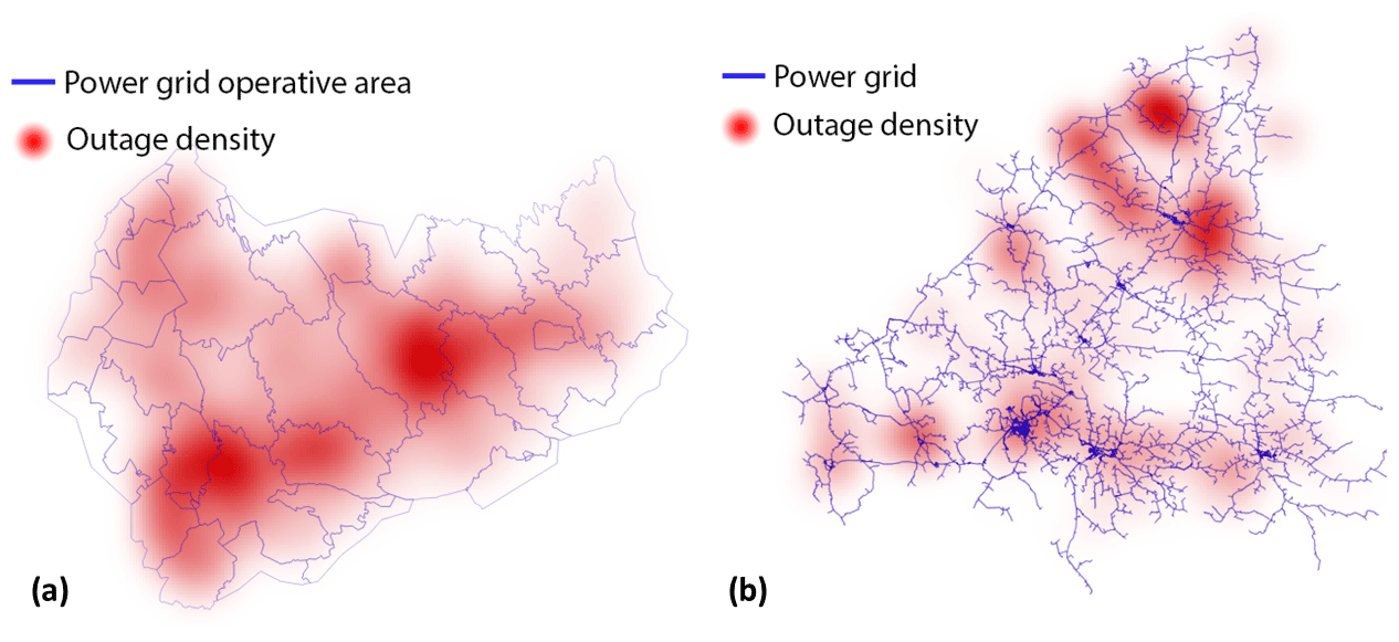
Figure 2Spatial distribution of the outages between 2010 and 2018 visualized as a spatial heat map. (a) JSE network (southern area) and (b) Loiste network (northern area).
It should be noticed that the damage may occur anywhere in the power grid. Outages are, however, always reported as transformers without electricity. Typically one instance of physical damage between the transformers causes several transformers to lose power. Power grid operators can often turn part of the transformers back to operation even before fixing the actual damage, which causes an unavoidable noise to the datasets.
Figure 3 represents the number of outages and storm objects in both local and national datasets. We can identify a large number of 15 m s−1 storm objects in both sets, indicating that moderate wind without other influencing factors does not damage the transformers. When identifying storm objects with the contour of 20 and 25 m s−1, the number of objects decreases and starts to correlate more with a high number of outages, which supports views of previous studies showing the significance of stronger wind gusts to more severe storm damage. The method seems to also identify the most critical storm days by capturing several storm objects for those days. For instance, at the end of 2013, when the three major storms Eino, Oskari, and Seija (Valta et al., 2019) hit Finland, both datasets contain plenty of storm objects with the 20 m s−1 threshold. Nevertheless, our experiments indicated that employing 15 m s−1 storm objects yielded the best results. This is described more in Sect. 4.
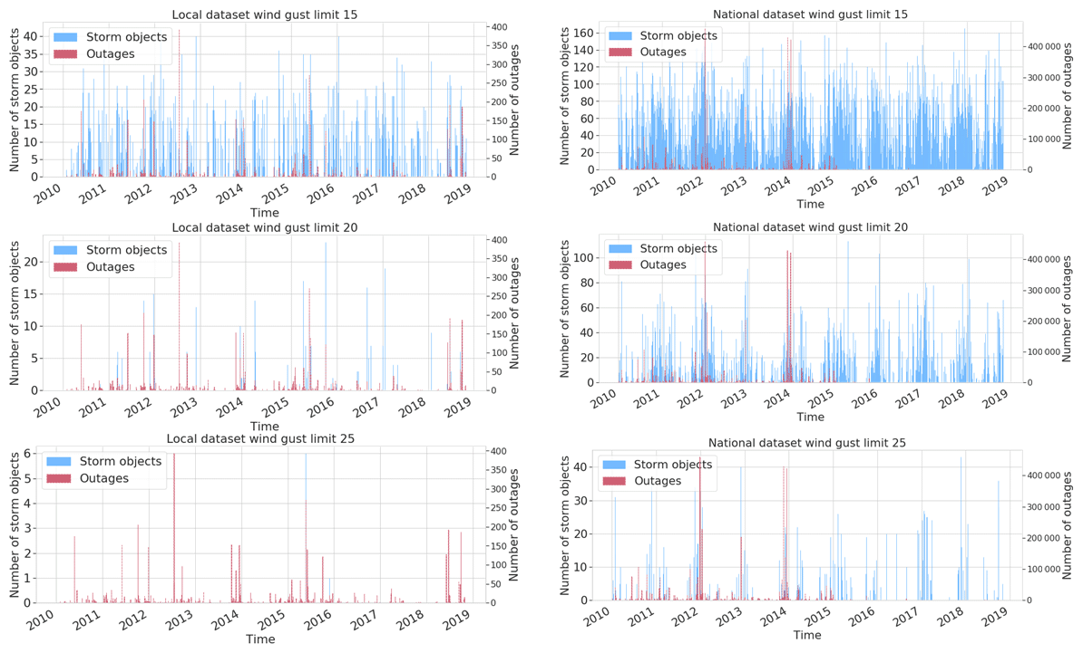
Figure 3Storm object time series (15, 20, and 25 m s−1 contours) with occurred outages for local and national datasets.
Figure 4 illustrates how many outages a single storm object typically produces. In the local dataset, most of the storm objects cause only a few outages. Only 65 storm objects, which are only 0.3 % of the whole dataset, induced more than 10 outages. On the other hand, in the national dataset where one storm object typically affects several different transformers, 17 587 storm objects have caused more than 10 outages, representing 12 % of the whole dataset. Figure 5 renders how many customers are typically affected by one outage. The figure contains all outages in both datasets, whether they are related to a storm or not. In the local dataset, usually 20–30 customers lose electricity in one outage. In the national dataset, only six customers usually lose electricity in one outage. We assume that this is due to different network topologies between the areas. Notably, in some rare cases, a much higher number of customers are affected. We assume that these cases typically occur in urban areas and are rare because the power network is mainly underground in these areas.
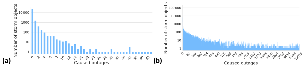
Figure 4Number of storm objects per caused outage in the (a) local dataset and (b) national dataset.
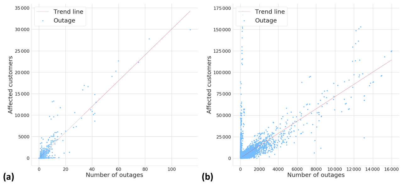
Figure 5Relationship between number of outages and affected customers in the (a) local dataset and (b) national dataset.
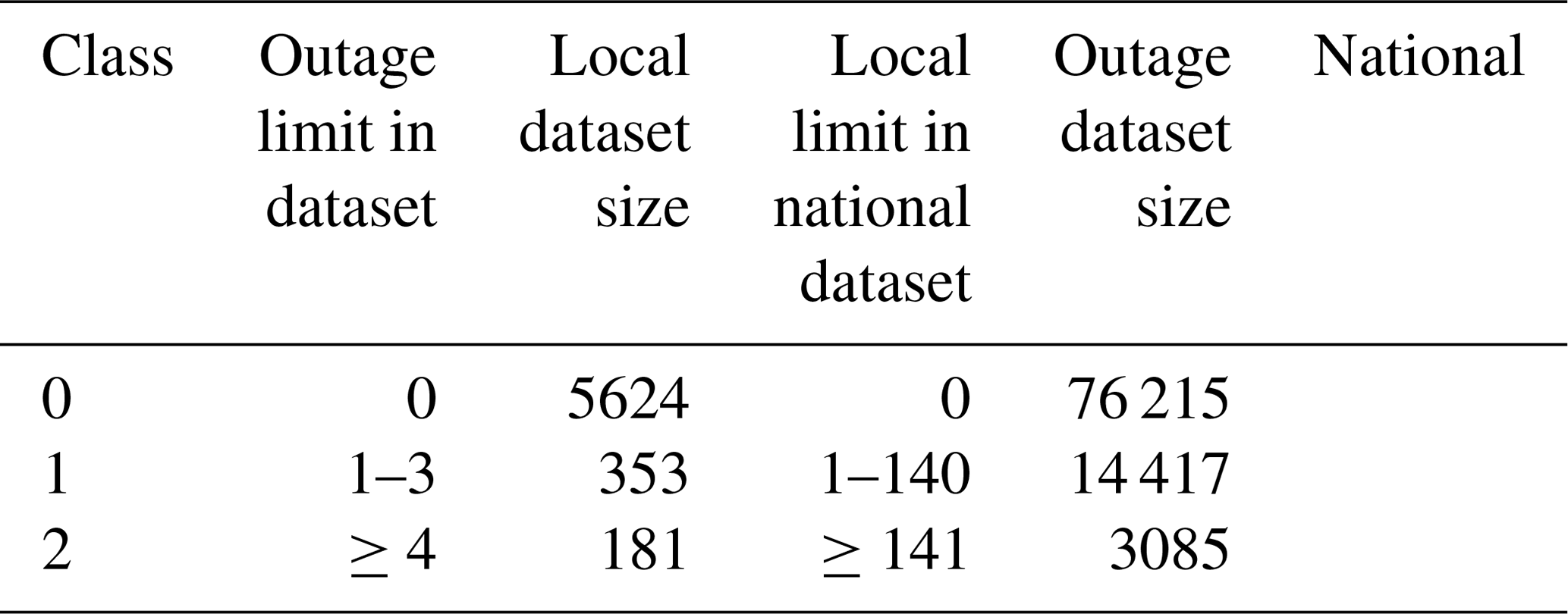
We use three classes designed together with power grid companies aiming at a simple “at glance” view for power grid operators. Class 0 represents no damage, class 1 low damage, and class 2 high damage. As the number of outages produced by a single storm object varies significantly in the local and national datasets, we decided to define separate limits for the local and the national datasets. The detailed limits are listed in Table 2. Class 1 is defined such that it represents roughly 80 % of all cases with at least one outage. Class sizes are highly imbalanced as most of the storm objects do not cause any damage.
3.4 Classifying storm objects
We centered and normalized the data points by subtracting the empirical mean and then dividing it by the empirical standard deviation. The hyperparameters were determined using random-search five-fold cross-validation (Bergstra and Bengio, 2012). To cope with the imbalanced class distribution, we generate artificial training samples using the synthetic minority over-sampling technique (SMOTE) (Chawla et al., 2002). SMOTE creates new training samples based on their k=5 nearest neighbors following
where xi is an original class sample, xzi is one of xi's k nearest neighbors, and λ is a random variable drawn uniformly from the interval [0, 1]. After augmentation, all classes have an equal number of samples, which reduces the tendency of classification methods to always predict the majority class.
Five different models were evaluated to classify storm objects. We omit the mathematical definitions but shortly discuss the characteristics of different models and describe the implementation details chosen in this work.
3.4.1 Random forest classification (RFC)
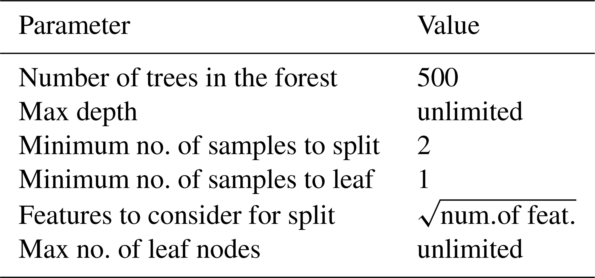
RFC is based on a random ensemble of decision trees and aggregating results from individual trees to the final estimate. Trees in the ensemble are constructed with four steps: (1) use bootstrapping to generate a random sample of the data, (2) randomly select a subset of features at each node, (3) determine the best split at the node using loss function, and (4) grow the full tree (Breiman, 2001). RFC is good to cope with high-dimensional data. It has also been found to provide adequate performance with imbalanced data (Tervo et al., 2019; Brown and Mues, 2012) and is widely used with weather data (e.g., Karthick et al., 2020; Cerrai et al., 2019; Lagerquist et al., 2017). The method is prone to overfit, which is why hyperparameter tuning is very important. Hyperparameters used in this work are listed in Table 3. We use RFC with the Gini impurity loss function.
3.4.2 Support vector classifiers (SVCs)
SVCs construct a hyperplane or classification function in a high-dimensional feature space and maximize a distance between training samples and the hyperplane. The hyperplanes may be constructed with nonlinear kernels such as the Gaussian radial basis function (RBF) (Shawe-Taylor and Cristianini, 2004) that often reform a nonlinear classification problem to a linear one. Operating in the high-dimensional feature space without additional computational complexity makes SVCs an attractive choice to extract meaningful features from a high-dimensional dataset. A domain-specific expert knowledge can also be capitalized on the kernel design. On the other hand, finding the correct kernel is often a difficult task. Training SVCs is a convex optimization problem, meaning that it has no local minima. Depending on the kernel, a training process may, however, be a very memory-intensive process.
Suppose the SVC output is assumed to be the log odds of a positive sample. In that case, one can fit a parametric model to obtain the posterior probability function and thus get probabilities for samples to belong to the particular class (Platt, 1999). For more details, we request the reader to consult for example Chang and Lin (2011) and Platt (1999).
We implement the SVCs in two phases. First, we separate class 0 (no outages) and other samples employing SVCs with the radial basis function (RBF), defined in Eq. (2). Second, we distinguish classes 1 and 2 using SVCs with a dot-product kernel defined in Eq. (3) (Williams and Rasmussen, 2006). The second phase is performed only for the samples predicted to cause outages in the first phase. The approach is similar to the often-used one-vs.-one classification, where a binary classifier is fitted for each pair of classes. In our case different kernels were used for different pairs.
where x and x′ are two samples in the input space and γ is a kernel coefficient parameter.
where x and x′ are two samples in the input space and σ is a kernel inhomogeneity parameter.
3.4.3 Gaussian naïve Bayes (GNB)
GNB (Chan et al., 1982) is a well-known and widely used method based on the Bayesian probability theory. The method assumes that all samples are independent and identically distributed (i.i.d.), which does not naturally hold for the weather data. Despite the internal structure of the data, GNB is still used for weather data (e.g., Kossin and Sitkowski, 2009; Cintineo et al., 2014; Karthick et al., 2020) and worth investigating in this context. The classification rule in GNB is , where P(y) is a frequency of class y and P(xi|y) is a likelihood of the ith feature assumed to be Gaussian. Because of the naïve i.i.d. assumption, each likelihood can be estimated separately, which helps to cope with a curse of dimensionality and enable GNB to work relatively well with small datasets. On the other hand, estimating likelihoods can be done effectively and iteratively, enabling the GNB to scale to large datasets. As a downside, the simple method may lack expression power to perform well in a complex context.
3.4.4 Gaussian processes (GPs)
The GP (Rasmussen, 2003) is a non-parametric probabilistic method that interprets the observed data points as realizations of a Gaussian random process. The GP is widely used for example in weather observation interpolation kriging (Holdaway, 1996). The GP is a very flexible and powerful but computationally expensive method, which tends to lose its power with high-dimensional data. The GP hinges on a kernel function that encodes the covariance between different data points. As a kernel, we use a product of a dot-product kernel (Eq. 3) and pairwise kernel with Laplacian distance (Rupp, 2015), defined in Eq. (4). The kernel parameters were optimized on the training data by maximizing the log-marginal likelihood.
where x and x′ are two samples in the input space and γ is a kernel coefficient parameter.
3.4.5 Multilayer perceptrons (MLPs)
MLPs (Goodfellow et al., 2016) are the most basic form of artificial neural networks. With good results achieved by MLPs in predicting storms (Ukkonen and Mäkelä, 2019), they are a natural choice for experimentation in this work. Neural networks are very adaptive methods as they can learn a representation of the input at their hidden layers. Unlike GNBs, they do not make any assumptions about the distribution of the data. As a downside, MLPs require large amounts of data, and the training process is computing-intensive. They also have a large number of hyperparameters to be optimized, including the correct network topology.
We searched the correct model parameters and network topology for local and national datasets by running multiple iterations of random-search five-fold cross-validation to obtain the best possible micro-average of the F1 score (defined in Sect. 4) employing the Talos library (Autonomio, 2020). The final setup is composed of a Nadam optimizer (Dozat, 2016), random normal initializer, and ReLU activation function for hidden layers. Binary cross-entropy was used as a loss function. Optimal network topology varied in different datasets: for the local dataset, the best results were obtained with a network containing three hidden layers with 75, 145, and 35 neurons. For the national dataset, the best results were obtained with a network containing three hidden layers with 75, 195, and 300 neurons. During the optimization process, the results varied between different setups from 0.6 to 0.95 in terms of the F1 score.
We used two different methods for splitting the data into training and test sets. The first method is uses 25 % of randomly picked samples in the test set. The second method is to construct a test set from a 1-year continuous time range (2010–2011). Both approaches have their advantages. A continuous time range ensures that the model has not seen any autocorrelated samples caused by an internal structure of the weather data in the training phase (Roberts et al., 2017). However, having only 9 years of data from a relatively small geographical area, the continuous test set cannot contain many storms as most of the data need to be reserved for the training process. Thus, the test set may only contain a single type of storm for which the model may work especially well or bad. Picking the test set randomly minimizes this risk and provides more insight into the model performance.
We evaluate the models with a weighted average of precision and recall and both weighted and macro-averages of the F1 score. Precision (Eq. 5) reports how many samples are correctly predicted to belong to a class. Recall (Eq. 6) tells how many samples belonging to a class are found in the prediction. The F1 score (Eqs. 7 and 8) calculates a harmonic mean of precision and recall. Finally, as the datasets are extremely imbalanced, we calculate a weighted average of the metrics utilizing a number of samples in each class and a macro-average of the F1 score using an average of the F1 score of each class. A model with a higher macro-average of the F1 score performs better with small classes. The selected metrics do not take a distance between predicted and true class into account. It is naturally worse to predict, for example, class 0 (no damage) in the case of a true class 2 (high damage) than in the case of a true class 1 (low damage). We decided, however, to use metrics that measure the method performance properly with imbalanced classes.
where 𝒞 represents the set of classes, predicted the class, “tp” is true positives, and “fp” is false positives.
where 𝒞 represents the set of classes, predicted the class, “tp” is true positives, and “fn” is false negatives.
where 𝒞 represents the set of classes, predicted the class, precision is defined in Eq. (5), and recall is defined in Eq. (6).
where 𝒞 represents the set of classes, precision is defined in Eq. (5), and recall is defined in Eq. (6).
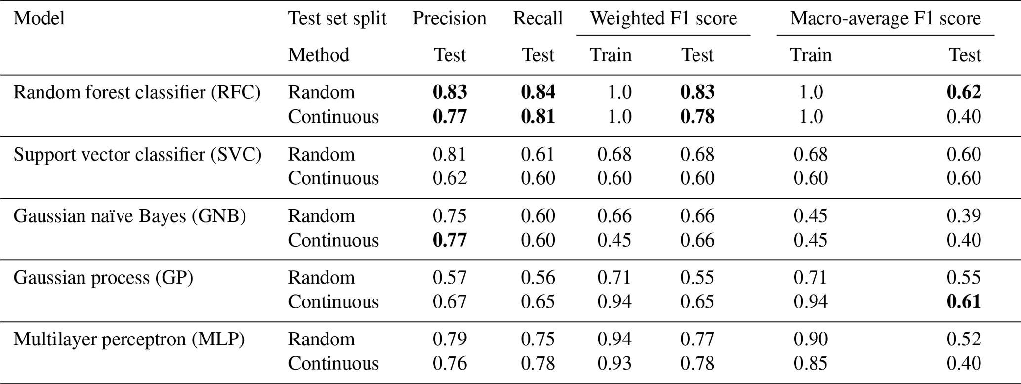
Tables 4 and 5 divulge the results for each model using the local and national datasets, respectively. Models trained with the local dataset can reach the better-weighted F1 score, while the best models trained with the national dataset provide a significantly better macro-average of the F1 score. The national dataset contains many more samples in classes 1 and 2, which enables models to learn the classes better and thus enhance the macro-average of the F1 score. Whether the test set is randomly chosen or continuous does not seem to make a large difference in most cases. The only affected model is the RFC, having contradictory better results trained with the continuous test set from the local dataset and the random test set from the national dataset. This reveals more about the unstable performance of RFC than the relevance of the dataset split method.
Table 4Results for each model trained with the local dataset obtained from two local power grid companies (defined in Sect. 3.3). The results with boldfaced font represent the best achieved results within the metric, shown separately for the random and continuous split methods.
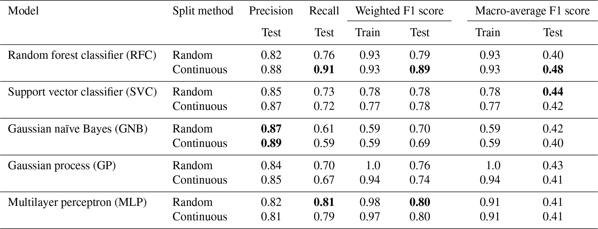
Table 5Results for each model trained with the national dataset covering all of Finland (defined in Sect. 3.3). The results with boldfaced font represent the best achieved results within the metric, shown separately for the random and continuous split methods.
The confusion matrices are depicted in Fig. 6. RFC provides the best results in terms of the selected metrics. However, closer exploration reveals that this performance is largely due to the best performance in predicting class 0, which is the largest class. SVC results are some of the most balanced ones, being the best only in the local dataset with a random test set but yielding good stable results in all cases. The confusion matrix, shown in Fig. 6b, displays that it is not the best model to predict class 0, but only a small share of true class 2 cases and the smallest share of true class 1 cases are predicted as class 0. That is to say, SVCs miss the smallest number of destructive storms, although it confuses the amount of caused damage.

Figure 6Confusion matrices produced using the randomly selected national dataset and (a) RFC, (b) SVC, (c) GNB, (d) GP and (e) MLP. Each cell of the confusion matrices represents a share of predictions having a corresponding combination of predicted and true class. For example, the middle right cell tells the share of samples belonging to class 1 but predicted to have class 2.
The GP is another strong option that performs even better with class 0 while still providing good performance with class 2. A significant connecting aspect between the GP and SVCs is an almost identical kernel. Based on these experiments, RBF and pairwise kernels separate harmless and harmful samples from each other while the dot-product kernel separates classes 1 and 2 even better than exponential functions. We select the GP for further analysis in this paper since it provides the best performance in class 2.
Using the 15 m s−1 threshold for detecting storm objects yields clearly better results than the 20 m s−1 threshold. For example, SVCs trained with the national dataset using the 20 m s−1 threshold and randomly chosen test set provide only a 0.48 macro-average of the F1 score, 12 percentage points below the corresponding model using the 15 m s−1 threshold. The 15 m s−1 threshold has two major advantages compared to the 20 m s−1 threshold. First, it provides a significantly larger dataset, and second, in contrast to the 20 m s−1 threshold, it is able to catch virtually all extratropical storms that cause outages.
4.1 Feature importance in the model performance
The relevance of the individual predictive features can be explored by using the permutation test, as done by Breiman (2001). First, the baseline score of the fitted model is calculated using the test set. Then each feature is randomly permuted, and the difference in the scoring function is calculated. The random permutation is repeated 30 times for each parameter, and the average of the results is used. The procedure offers information on how important the feature is to obtain good results. It should be mentioned that highly correlated features may get low importance as other features work as a proxy to the permuted feature. However, using completely independent features is not possible in weather data since weather parameters are often dependent on each other, and eliminating even the most apparent pairs from the used features impaired the results in our experiments.
We used the macro-average of F1 defined in Eq. (8) as a scoring function and the randomly selected test set from the national data. The relevance is shown in Fig. 7. Most features show at least a little relevance for the results. The first 12 features are significantly more relevant than the rest. The most important features contain at least one representative of all meteorological parameters used in the training. In other words, all employed meteorological parameters are important for the prediction, while different aggregations contribute to the “fine-tuning” of the model.

Figure 7Permutation feature importance using the GP classification method trained with the randomly selected national dataset. The higher the effect on the F1 score (y axis), the bigger the significance.
As Fig. 7 shows, the most significant parameter regarding our model performance is the average wind speed. Numerous studies support our result of wind being the most important damaging factor (Virot et al., 2016; Valta et al., 2019; Jokinen et al., 2015). However, the studies highlight the importance of maximum wind gusts instead of the average wind. Surprisingly, in our analysis, the wind gust speed does not belong to the most critical parameters. Instead, maximum mixed-layer height, related to the wind gustiness, contributes crucially to the model performance. The dependencies between predictive features might be one reason for some parameters to have a lower rank in the results.
The stand mean diameter and height are the most important features regarding the forest parameters, which corresponds to our expectations. Previous studies also show these features influence the wind damage in forests (Pellikka and Järvenpää, 2003) and hence indirectly electricity grids. As Pellikka and Järvenpää (2003) and Suvanto et al. (2016) discuss, the age of the forest also has an impact on storm damage. However, in the feature importance test, forest age does not seem to contribute significantly to the prediction outcome.
The most important object feature is the size of the object. Object movement speed and direction did not contribute strongly to the results. However, previous studies indicate that besides the size of the impacted area, the duration of strong winds – i.e., the propagation speed of the system – also influences the amount of damage (Lamb and Knud, 1991).
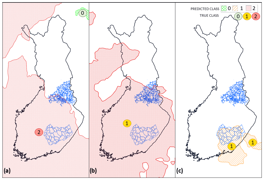
Figure 8Selected examples. (a) Extratropical storm Tapani (26 December 2011 11:00 UTC), (b) extratropical storm Rauli (27 August 2016 10:00 UTC), and (c) extratropical storm Pauliina (22 June 2018 01:00 UTC), produced by employing the SVC model trained with the national dataset. The storm objects are colored based on the predicted class while the true class is stated as a colored number over the object.
4.2 Case examples
We illustrate the prediction produced using the GP classification method with the three most interesting examples of well-known storms in Fig. 8. We chose the cases among a number of test cases to illustrate the strengths and weaknesses of the method. The examples are chosen from the randomly picked test set, which was not used to train the model. Because of the random sample, we cannot represent the entire prediction of individual storms, only individually picked time steps. In two of the example cases, the model performs well (storms Tapani and Pauliina) and in one case (storm Rauli) less accurately.
4.2.1 Event 1: extratropical storm Tapani (26 December 2011)
The first example is one of the most known extratropical storms in Finland. Storm Tapani, also known as Cyclone Dagmar (Kufeoglu and Lehtonen, 2015), was a rare winter storm, causing broad and long-lasting electricity interruptions. Extreme wind gusts of over 30 m s−1 caused widespread damage, especially in the southern and western parts of the country. Approximately 570 000 households were left without electricity, causing EUR 30 million of repair costs and EUR 80 million of monetary compensation for electricity distribution companies to their customers (Hanninen and Naukkarinen, 2012). An exceptionally warm December and the warmest Boxing Day in 50 years (Finnish Meteorological Institute, 2011) resulted in wet and unfrozen soil. Thus, the trees were poorly anchored and exposed to significant storm damage.
Figure 8a represents the outage prediction (raster-covered areas) and the actual true classes (numbers) based on the damage data at 15:00 UTC, 26 December 2011. Wide areas in central and western parts of Finland are predicted to have high (class 2) damage. The predicted class is in line with the true class. Also, the damage areas of the storm correlate with the wind gust observations of the Finnish Meteorological Institute. The strongest gusts occurred in western (15–27 m s−1) and southern (18–28 m s−1) Finland and the northwestern part of Lapland (13–31 m s−1) (Finnish Meteorological Institute, 2020). In the rest of Finland, the maximum wind gusts remained between 10–15 m s−1, and therefore the damage were minor. Overall, the model predicted the damage accurately in this particular example.
4.2.2 Event 2: extratropical storm Rauli (27 August 2016)
Extratropical storm Rauli was an exceptionally strong summer storm, especially regarding the impacts. It caused severe damage to the power grid in the western and middle parts of Finland for various reasons. The trees still carried leaves, the soil was wet after a rainy August, the strong wind areas of Rauli were widespread, and the solar radiation intensified the wind gusts during the afternoon (Finnish Meteorological Institute, 2016). Rauli impacted the middle and southern parts of Finland in particular, which are also the most densely populated areas. The power outages increased rapidly in the middle part of Finland, starting at midday and reaching the highest values, 200 000 households without electricity (Ilta-Sanomat, 2016), around 17:00 UTC. The winds blew exceptionally long, nearly 24 h. The typical duration of summer storms is between 6–12 h.
Figure 8b shows the predicted outages and true classes at 12:00 UTC, 27 August 2016. In this particular time step, the model overpredicts the class; however, the predicted outage area seems to correlate with the wind gust maxima of that afternoon. The strongest wind gusts were measured in the southern and middle parts of the country, with maximum gusts reaching up to 24.9 m s−1 at land stations (Klemettilä, Vaasa and Maaninka, Pohjois-Savo) and in wide areas up to 20 m s−1 apart from the northern part of Finland.
4.2.3 Event 3: extratropical storm Pauliina (22 June 2018)
The last example is a strong extratropical storm, called Pauliina (Finnish Meteorological Institute, 2018), that caused numerous power outages in Finland. The most significant part of the power outages happened in the network of the power grid company JSE included in the local dataset. The highest peak in the damage was reached between 18:00 and 20:00 UTC with over 28 000 households without electricity. The strongest wind gust on land reached 22.7 m s−1 in Helsinki, Kumpula observation station, and the inland gusts were widely between 15–20 m s−1 (Finnish Meteorological Institute, 2020; Finnish Meteorological Institute – Twitter, 2020). The strong wind gusts continued until the dawn of 23 June.
Figure 8c presents the predicted and true damage classes at 01:00 UTC, 22 June 2018. We chose extratropical storm Pauliina as an example storm for two reasons: (1) Pauliina represents a low-damage class and (2) Pauliina represents a rare, summer-season extratropical storm. Figure 8c shows the predicted and true classes correlating. While weather warnings were issued to large areas in the southern and middle parts of Finland, myrskyvaroitus.com (2018) predicted and true damage to the power grid occurred in a relatively small geographical area.
This paper introduces a novel method to predict the damage potential of extratropical storms to power grids. The method consists of identifying storm objects by contouring surface wind gust fields with the 15 m s−1 threshold along with pressure objects with a 1000 hPa threshold, tracking the objects, and then classifying them into three classes based on their damage potential to the power grid. For the classification task, we evaluated five different machine-learning methods, all employing a total of 35 predictive features and trained with 8 years of power outage data from Finland.
Both Gaussian processes and support vector classifiers provided good results. The model recognizes harmful storm objects well and can distinguish extremely harmful objects among others adequately. While the results still leave a lot to improve, the developed model can already be used to support decisions in power grid companies. In some cases, the model is able to provide a more specific and geospatially accurate prediction of potential damage to the power grid than, for example, weather warning. The evaluation was, however, based on the ERA5 reanalysis data. Using the method in an operational setting would require weather prediction data, which introduces additional uncertainty to the outage prediction.
The presented object-based approach has both advantages and disadvantages. Extracting storm objects in advance preprocesses the data for machine-learning techniques, such as RFC, which do not perform feature learning. It enables machine-learning methods to focus only on the relevant parts of the data. Methods not containing feature learning, such as RFC and logistic regression, have been found to outperform neural networks for forest (Hart et al., 2019) and weather data (Tervo et al., 2019). It also leads to significantly faster training times. Processing objects instead of the grid also makes it easier to track and use object attributes such as age, speed, and movement. Moreover, objects are easy to visualize, and user interfaces may be enriched with related actions such as tracking and alarms.
On the other hand, storm objects use only aggregated attributes, which may decrease the classification accuracy when predictive features vary significantly under the storm object area. Several machine-learning methods, i.e., deep neural networks, could be trained to employ those local features to gain better accuracy. Such methods could also utilize three-dimensional data.
The fixed thresholds of wind gust and pressure were used to extract the storm objects in this paper. Although the previous studies indicate the critical threshold of wind gust speed to be the same for almost the entire geospatial domain of this work (Gardiner et al., 2013), it would be beneficial to adapt the threshold based on the geographic location using, for example, the storm severity index (SSI) originally introduced in Leckebusch et al. (2008). Moreover, the correct threshold may vary depending on the data source.
The work opens several possible avenues for further studies. It would be interesting to compare the current solution with a grid-based approach and deep neural networks. Including data on soil moisture, soil temperature, and leaf index would most likely enhance the results, if available with sufficient spatial and temporal resolution, since they would provide critical information about the environmental conditions. Different thresholds could be investigated as well, especially for pressure objects where lower thresholds might yield better results. By design, applying the method to other regions is possible, but it is subject to the availability of power outage records, forest inventory, impact, and meteorological data. For the classification task, carefully designed Bayesian networks could provide good results as well. Especially in the randomly selected test set, data may be autocorrelated, which may lead to unrealistically good results. We have addressed this issue by also using a continuous time series (from 2010 to 2011) for the test set. The evaluation could also be extended with a leave-one-day-out or leave-one-week-out method where for each week 1 d or for each month 1 week is left out for validation purposes.
End users, especially expert users like duty forecasters, might benefit from the uncertainty information originating as the probabilistic prediction of the classification model. However, the presentation of such information should be very carefully chosen to not mislead non-expert users for overconfidence.
Experiments in this study were conducted with ERA5 reanalysis and additional forest data. As the method employs common features also existing in various other datasets, data provided by other vendors could be used as well. By employing weather forecasts as input, this method could be used as a base for a decision support tool and as part of an existing early warning system for both duty forecasters of national hydro-meteorological centers and operators of electricity transmission companies.
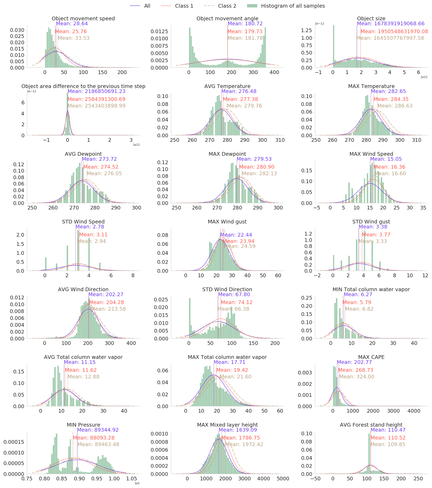
Figure A1Histogram of and fitted Gaussian distribution of selected predictive parameters in the local dataset. The Gaussian distribution is fitted separately to all samples and samples with little outages and many outages (classes 1 and 2 specified in Sect. 3.3).
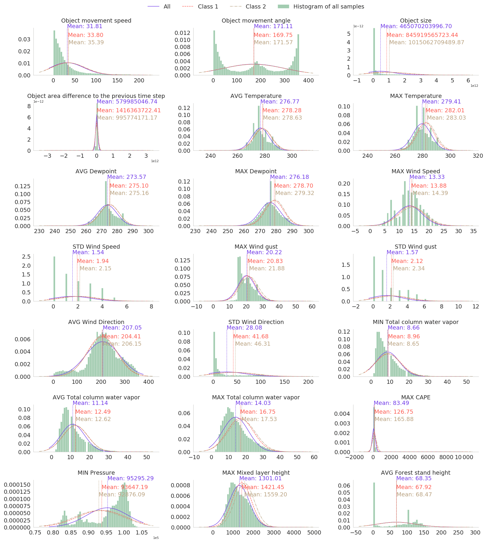
Figure A2Histogram of and fitted Gaussian distribution of selected predictive parameters in the national dataset. The Gaussian distribution is fitted separately to all samples and samples with little outages and many outages (classes 1 and 2 specified in Sect. 3.3).
The source code is available in the repositories https://doi.org/10.5281/zenodo.4525236 (Tervo and Sirviö, 2020a) and https://doi.org/10.5281/zenodo.4525234 (Tervo, 2020).
ERA5 data may be downloaded from the Copernicus Climate Data Store: https://doi.org/10.24381/cds.bd0915c6 (Hersbach et al., 2018). The forest inventory may be downloaded from the LUKE open data service: http://kartta.luke.fi/index-en.html (last access: 20 February 2019) (Korhonen et al., 2019). The power outage data are proprietary data for which the authors have no property rights to distribute.
RT conceptualized, designed, and developed the method. IL contributed with meteorological expertise, such as selecting used data and meteorological features along with correct thresholds. IL also helped in analyzing the performance. AM provided supervision from a meteorological perspective and AJ from a machine-learning perspective. All contributed in presenting the results.
The authors declare that they have no conflict of interests.
The authors express their gratitude to Järvi-Suomen Energia, Loiste Sähköverkko, and Imatran Seudun Sähkönsiirto for sharing data and their experience.
This paper was edited by Amy Donovan and reviewed by Tim Kruschke and one anonymous referee.
Allen, M., Fernandez, S., Omitaomu, O., and Walker, K.: Application of hybrid geo-spatially granular fragility curves to improve power outage predictions, J. Geogr. Nat. Disast., 4, 1–6, https://doi.org/10.4172/2167-0587.1000127, 2014. a
Autonomio: Talos (software), available at: http://github.com/autonomio/talos., last access: 22 June 2020. a
Barredo, J. I.: Normalised flood losses in Europe: 1970–2006, Nat. Hazards Earth Syst. Sci., 9, 97–104, https://doi.org/10.5194/nhess-9-97-2009, 2009. a
Bergstra, J. and Bengio, Y.: Random search for hyper-parameter optimization, J. Mach. Learn. Res., 13, 281–305, 2012. a
Breiman, L.: Random forests, Mach. Learn., 45, 5–32, 2001. a, b
Brown, I. and Mues, C.: An experimental comparison of classification algorithms for imbalanced credit scoring data sets, Exp. Syst. Appl., 39, 3446–3453, 2012. a
Campbell, R. J. and Lowry, S.: Weather-related power outages and electric system resiliency, Tech. rep., Congressional Research Service, Library of Congress, Washington, D.C., 2012. a
Cerrai, D., Wanik, D. W., Bhuiyan, M. A. E., Zhang, X., Yang, J., Frediani, M. E., and Anagnostou, E. N.: Predicting storm outages through new representations of weather and vegetation, IEEE Access, 7, 29639–29654, 2019. a, b
Chan, T. F., Golub, G. H., and LeVeque, R. J.: Updating formulae and a pairwise algorithm for computing sample variances, in: COMPSTAT 1982 5th Symposium held at Toulouse 1982, 30–41, https://doi.org/10.1007/978-3-642-51461-6, 1982. a
Chang, C.-C. and Lin, C.-J.: LIBSVM: A library for support vector machines, ACM Trans. Intel. Syst. Technol., 2, 27, https://doi.org/10.1145/1961189.1961199, 2011. a
Chawla, N. V., Bowyer, K. W., Hall, L. O., and Kegelmeyer, W. P.: SMOTE: synthetic minority over-sampling technique, J. Artif. Intel. Res., 16, 321–357, 2002. a
Chen, P.-C. and Kezunovic, M.: Fuzzy logic approach to predictive risk analysis in distribution outage management, IEEE T. Smart Grid, 7, 2827–2836, 2016. a
Chen, S. H., Jakeman, A. J., and Norton, J. P.: Artificial intelligence techniques: an introduction to their use for modelling environmental systems, Math. Comput. Simul., 78, 379–400, 2008. a
Cintineo, J. L., Pavolonis, M. J., Sieglaff, J. M., and Lindsey, D. T.: An empirical model for assessing the severe weather potential of developing convection, Weather Forecast., 29, 639–653, 2014. a, b, c
Csilléry, K., Kunstler, G., Courbaud, B., Allard, D., Lassegues, P., Haslinger, K., and Gardiner, B.: Coupled effects of wind-storms and drought on tree mortality across 115 forest stands from the Western Alps and the Jura mountains, Global Change Biol., 23, 5092–5107, https://doi.org/10.1111/gcb.13773, 2017. a
Donat, M. G., Leckebusch, G. C., Wild, S., and Ulbrich, U.: Future changes in European winter storm losses and extreme wind speeds inferred from GCM and RCM multi-model simulations, Nat. Hazards Earth Syst. Sci., 11, 1351–1370, https://doi.org/10.5194/nhess-11-1351-2011, 2011. a
Dozat, T.: Incorporating nesterov momentum into adam, in: 4th International Conference on Learning Representations, 2–4 May 2016, San Juan, Puerto Rico, available at: https://openreview.net/pdf?id=OM0jvwB8jIp57ZJjtNEZ (last access: 10 February 2021), 2016. a
Eskandarpour, R. and Khodaei, A.: Machine Learning Based Power Grid Outage Prediction in Response to Extreme Events, IEEE T. Power Syst., 32, 3315–3316, 2017. a
European Centre for Medium-Range Weather Forecasts: ERA5: large 10 m winds, available at: https://confluence.ecmwf.int/display/CKB/ERA5:+large+10m+winds (last access: 10 May 2020), 2019. a
Finnish Energy: Energy distribution interruptions 2010–2018 – Finnish Energy, available at: https://energia.fi/julkaisut/materiaalipankki/sahkon_keskeytystilastot_2010-2018.html#material-view (last access: 8 May 2020), 2010–2018. a, b
Finnish Energy: Energy distribution interruptions 2011 – Finnish Energy, Tech. rep., Finnish Energy, available at: https://energia.fi/files/605/Keskeytystilasto_2011.pdf (last access: 16 February 2020), 2011. a
Finnish Energy: Energy distribution interruptions 2013 – Finnish Energy, Tech. rep., Finnish Energy, available at: https://energia.fi/files/605/Keskeytystilasto_2013.pdf (last access: 4 June 2020), 2013. a
Finnish Meteorological Institute: Climate Statistics Report (December 2011), Helsinki, Finland, 1–24, 2011. a
Finnish Meteorological Institute: Rauli nousi myrskyjen raskaaseen sarjaan | Ilmastokatsaus – Ilmatieteen laitos, Ilmastokatsaus, available at: http://www.ilmastokatsaus.fi/2016/08/29/rauli-nousi-myrskyjen-raskaaseen-sarjaan/ (last access: 15 June 2020), 2016. a
Finnish Meteorological Institute: Kesäkuun 2018 kuukausikatsaus | Ilmastokatsaus – Ilmatieteen laitos, available at: http://www.ilmastokatsaus.fi/2018/07/04/kesakuun-2018-kuukausikatsaus/ (last access: 15 June 2020), 2018. a
Finnish Meteorological Institute: Open data, observation download service, available at: https://en.ilmatieteenlaitos.fi/download-observations, last access: 15 June 2020. a, b
Finnish Meteorological Institute – Twitter: Ilmatieteen laitos Twitterissä: “#Juhannus'aaton-#myrsky #Pauliina lukuina klo 15.30: kovin puuska 32,5 m/s ja 10min keskituuli 26,5 m/s (Kaskinen Sälgrund), maa-alueilla Helsinki Kumpula puuska 22,7 m/s. Vaasa Klemettilä 24 h sademäärä 41 mm.”/Twitter, available at: https://twitter.com/meteorologit/status/1010144460703969280, last access: 17 June 2020. a
Gardiner, B., Blennow, K., Carnus, J., Fleischner, P., Ingemarson, F., Landmann, G., Lindner, M., Marzano, M., Nicoll, B., Orazio, C., Peyron, J., Reviron, M., Schelhaas, M., Schuck, A., Spielmann, M., and Usbeck, T.: Destructive storms in European Forests: Past and Forthcoming Impacts. Final report to European Commission – DG Environment, European Forest Institute, Wageningen, the Netherlands, 2010. a, b
Gardiner, B., Schuck, A., Schelhaas, M.-J., Orazio, C., Blennow, K., and Nicoll, B.: Living with Storm Damage to Forests What Science Can Tell Us What Science Can Tell Us, European Forest Institute, EFI, Joensuu, Finland, https://doi.org/10.13140/2.1.1730.2400, 2013. a, b
Goodfellow, I., Bengio, Y., and Courville, A.: Deep Learning, in: Deep Learning, MIT Press, Cambridge, Massachusetts, USA, 164–223, 2016. a
Govorushko, S. M.: Natural processes and human impacts: Interactions between humanity and the environment, Springer Science & Business Media, the Netherlands, 2011. a, b
Gregow, H., Laaksonen, A., and Alper, M. E.: Increasing large scale windstorm damage in Western, Central and Northern European forests, 1951–2010, Scient. Rep., 7, 46397, https://doi.org/10.1038/srep46397, 2017. a
Guikema, S. D., Quiring, S. M., and Han, S. R.: Prestorm Estimation of Hurricane Damage to Electric Power Distribution Systems, Risk Anal., 30, 1744–1752, https://doi.org/10.1111/j.1539-6924.2010.01510.x, 2010. a
Guikema, S. D., Nateghi, R., Quiring, S. M., Staid, A., Reilly, A. C., and Gao, M.: Predicting Hurricane Power Outages to Support Storm Response Planning, IEEE Access, 2, 1364–1373, https://doi.org/10.1109/ACCESS.2014.2365716, 2014. a
Haarsma, R. J., Hazeleger, W., Severijns, C., De Vries, H., Sterl, A., Bintanja, R., Van Oldenborgh, G. J., and Van Den Brink, H. W.: More hurricanes to hit western Europe due to global warming, Geophys. Res. Lett., 40, 1783–1788, https://doi.org/10.1002/grl.50360, 2013. a
Han, S. R., Guikema, S. D., and Quiring, S. M.: Improving the predictive accuracy of hurricane power outage forecasts using generalized additive models, Risk Anal., 29, 1443–1453, https://doi.org/10.1111/j.1539-6924.2009.01280.x, 2009. a
Hanewinkel, M.: Neural networks for assessing the risk of windthrow on the forest division level: a case study in southwest Germany, Eur. J. Forest Res., 124, 243–249, 2005. a
Hanninen, K. and Naukkarinen, J.: 570 000 customers experienced power losses at the end of the year, (Loppuvuoden sähkökatkoista kärsi 570 000 asiakasta – Energiateollisuus, available at: http://www.mynewsdesk.com/fi/pressreleases/loppuvuoden-saehkoekatkoista-kaersi-570-000-asiakasta-725038 (last access: 11 June 2020), 2012. a
Hart, E., Sim, K., Kamimura, K., Meredieu, C., Guyon, D., and Gardiner, B.: Use of machine learning techniques to model wind damage to forests, Agr. Forest Meteorol., 265, 16–29, 2019. a, b
He, J., Wanik, D. W., Hartman, B. M., Anagnostou, E. N., Astitha, M., and Frediani, M. E.: Nonparametric Tree-Based Predictive Modeling of Storm Outages on an Electric Distribution Network, Risk Anal., 37, 441–458, https://doi.org/10.1111/risa.12652, 2017. a
Hersbach, H., Bell, B., Berrisford, P., Biavati, G., Horányi, A., Muñoz Sabater, J., Nicolas, J., Peubey, C., Radu, R., Rozum, I., Schepers, D., Simmons, A., Soci, C., Dee, D., and Thépaut, J.-N.: ERA5 hourly data on pressure levels from 1979 to present, Copernicus Climate Change Service (C3S) Climate Data Store (CDS), https://doi.org/10.24381/cds.bd0915c6, 2018. a, b
Hersbach, H., Bell, W., Berrisford, P., Horányi, A. J. M.-S., Nicolas, J., Radu, R., Schepers, D., Simmons, A., Soci, C., and Dee, D.: Global reanalysis: goodbye ERA-Interim, hello ERA5, ECMWF newsletter, European Centre for Medium-Range Weather Forecasts, Reading, UK, 17–24, https://doi.org/10.21957/vf291hehd7, 2019. a, b
Holdaway, M. R.: Spatial modeling and interpolation of monthly temperature using kriging, Clim. Res., 6, 215–225, 1996. a
Ilta-Sanomat: Rauli-myrsky repii Suomea: lähes 200000 taloutta ilman sähköjä – Kotimaa – Ilta-Sanomat, available at: https://www.is.fi/kotimaa/art-2000001248969.html (last access: 15 June 2020), 2016. a
IPCC: Impacts of 1.5 ∘C global warming on natural and human systems, Global warming of 1.5 ∘C, An IPCC Special Report, Intergovernmental Panel on Climate Change, Geneva, Swizerland, 2018. a
Jokinen, P., Vajda, A., and Gregow, H.: The benefits of emergency rescue and reanalysis data in decadal storm damage assessment studies, Adv. Sci. Res., 12, 97–101, https://doi.org/10.5194/asr-12-97-2015, 2015. a
Kankanala, P., Pahwa, A., and Das, S.: Regression models for outages due to wind and lightning on overhead distribution feeders, in: 2011 IEEE Power and Energy Society General Meeting, 24–28 July 2011, Detroit, Michigan, USA, 1–4, 2011. a
Kankanala, P., Pahwa, A., and Das, S.: Estimation of Overhead Distribution System Outages Caused by Wind and Lightning Using an Artificial Neural Network, in: International Conference on Power System Operation & Planning, 12–14 November 2012, Las Vegas, USA, 2012. a
Kankanala, P., Das, S., and Pahwa, A.: AdaBoost+: An Ensemble Learning Approach for Estimating Weather-Related Outages in Distribution Systems, IEEE T. Power Syst., 29, 359–367, 2014. a
Karthick, S., Malathi, D., Sudarsan, J., and Nithiyanantham, S.: Performance, evaluation and prediction of weather and cyclone categorization using various algorithms, Model. Earth Syst. Environ., https://doi.org/10.1007/s40808-020-00887-7, in press, 2020. a, b
Korhonen, K., Packalen, T., and Kangas, A.: The National Forest Inventory (NFI), available at: http://kartta.luke.fi/index-en.html, last access: 20 February 2019. a
Kossin, J. P. and Sitkowski, M.: An objective model for identifying secondary eyewall formation in hurricanes, Mon. Weather Rev., 137, 876–892, 2009. a
Kron, W. and Schuck A.: After the floods, Tech. rep., Münchener Rückversicherungs-Gesellschaft (Munich Reinsurance Company), available at: https://www.munichre.com/content/dam/munichre/global/content-pieces/documents/302-08121_en.pdf/_jcr_content/renditions/original./302-08121_en.pdf (last access: 5 June 2020), 2013. a
Kufeoglu, S. and Lehtonen, M.: Cyclone Dagmar of 2011 and its impacts in Finland, in: IEEE PES Innovative Smart Grid Technologies Conference Europe, vol. 2015-January, IEEE Computer Society, Istanbul, Turkey, https://doi.org/10.1109/ISGTEurope.2014.7028868, 2015. a, b
Lagerquist, R., McGovern, A., and Smith, T.: Machine learning for real-time prediction of damaging straight-line convective wind, Weather Forecast., 32, 2175–2193, 2017. a
Lamb, H. and Knud, F.: Historic Storms of the North Sea, British Isles and Northwest Europe – Google Books, available at: https://books.google.fi/books?hl=en&lr=&id=P4n1z9rOh5MC&oi=fnd&pg=PR8&ots=ewtYPSlQ1H&sig=VJJ00ehiPL0d1oaTDfa14nFb3zI&redir_esc=y#v=onepage&q=duration&f=false (last access: 30 September 2020), 1991. a
Leckebusch, G. C., Renggli, D., and Ulbrich, U.: Development and application of an objective storm severity measure for the Northeast Atlantic region, Meteorol. Z., 17, 575–587, https://doi.org/10.1127/0941-2948/2008/0323, 2008. a
Li, Z., Singhee, A., Wang, H., Raman, A., Siegel, S., Heng, F.-L., Mueller, R., and Labut, G.: Spatio-temporal forecasting of weather-driven damage in a distribution system, in: 2015 IEEE Power & Energy Society General Meeting, 26–30 July 2015, Denver, CO, USA, 1–5, 2015. a
Liu, Y., Zhong, Y., and Qin, Q.: Scene Classification Based on Multiscale Convolutional Neural Network, IEEE T. Geosci. Remote Sens., 56, 7109–7121, https://doi.org/10.1109/TGRS.2018.2848473, 2018. a
Mäkisara, K., Katila, M., Peräsaari, J., and Tomppo, E.: The multi-source national forest inventory of Finland – methods and results 2013, Natural Resources Institute Finland (Luke), Helsinki, Finland, 215 pp., ISBN 978-952-326-186-0, 2016. a
Masson-Delmotte, T., Zhai, P., Pörtner, H., Roberts, D., Skea, J., Shukla, P., Pirani, A., Moufouma-Okia, W., Péan, C., Pidcock, R., Connors, S., Matthews, J. B. R., Chen, Y., Zhou, X., Gomis, M. I., Lonnoy, E., Maycock, T., Tignor, M., and Waterfield, T.: IPCC, 2018: Summary for Policymakers, in: Global warming of 1.5 ∘C. An IPCC Special Report on the impacts of global warming of 1.5 ∘C above pre-industrial levels and related global greenhouse gas emission pathways, in the context of strengthening the global, Geneva, Switzerland, 2018. a
myrskyvaroitus.com: 2018 Syystrombeja, available at: https://myrskyvaroitus.com/index.php/myrskytieto/myrskyhistoria/202-2018-syystrombeja (last access: 18 June 2020), 2018. a
Nateghi, R., Guikema, S., and Quiring, S. M.: Power Outage Estimation for Tropical Cyclones: Improved Accuracy with Simpler Models, Risk Anal., 34, 1069–1078, https://doi.org/10.1111/risa.12131, 2014. a
Niemelä, E.: KESKEYTYSTILASTO 2017 (i), Tech. Rep. 2018-06-14 11:51:52.916, Energiateollisuus Ry, Helsinki, Finland, available at: https://energia.fi/files/2785/Sahkon_keskeytystilasto_2017.pdf (last access: 16 February 2020), 2018. a
Nurmi, V., Pilli-Sihvola, K., Gregow, H., and Perrels, A.: Overadaptation to Climate Change? The Case of the 2013 Finnish Electricity Market Act, Econ. Disast. Clim. Change, 3, 161–190, https://doi.org/10.1007/s41885-018-0038-1, 2019. a
Pellikka, P. and Järvenpää, E.: Forest stand characteristics and wind and snow induced forest damage in boreal forest, in: Proceedings of the International Conference on Wind Effects on Trees, held in September, 16–18, Citeseer, Karlsruhe, Germany, 2003. a, b
Peltola, H., Kellomäki, S., and Väisänen, H.: Model Computations of the Impact of Climatic Change on the Windthrow Risk of Trees, Climatic Change, 41, 17–36, https://doi.org/10.1023/A:1005399822319, 1999. a, b
Pinto, J. G., Bellenbaum, N., Karremann, M. K., and Della-Marta, P. M.: Serial clustering of extratropical cyclones over the North Atlantic and Europe under recent and future climate conditions, J. Geophys. Res.-Atmos., 118, 12476–12485, https://doi.org/10.1002/2013JD020564, 2013. a
Platt, J.: Probabilistic outputs for support vector machines and comparisons to regularized likelihood methods, Adv. Large Marg. Class., 10, 61–74, 1999. a, b
Ramon, J., Lledó, L., Torralba, V., Soret, A., and Doblas‐Reyes, F. J.: What global reanalysis best represents near‐surface winds?, Natural Disasters and Adaptation to Climate Change, 145, 3236–3251, https://doi.org/10.1002/qj.3616, 2019. a
Rasmussen, C. E.: Gaussian processes in machine learning, in: Summer School on Machine Learning, Springer, Cambridge, Massachusetts, USA, 63–71, 2003. a
Roberts, D. R., Bahn, V., Ciuti, S., Boyce, M. S., Elith, J., Guillera-Arroita, G., Hauenstein, S., Lahoz-Monfort, J. J., Schröder, B., Thuiller, W., Warton, D. I., Wintle, B. A., Hartig, F., and Dormann, C. F.: Cross-validation strategies for data with temporal, spatial, hierarchical, or phylogenetic structure, Ecography, 40, 913–929, https://doi.org/10.1111/ecog.02881, 2017. a
Rossi, P. J.: Object-Oriented Analysis and Nowcasting of Convective Storms in Finland, PhD thesis, Aalto University, available at: http://urn.fi/URN:ISBN:978-952-60-6441-3 (last access: 14 June 2020), 2015. a, b
Rupp, M.: Machine learning for quantum mechanics in a nutshell, Int. J. Quant. Chem., 115, 1058–1073, 2015. a
Schelhaas, M.-J.: Impacts of natural disturbances on the development of European forest resources: application of model approaches from tree and stand levels to large-scale scenarios, Dissertationes Forestales, Alterra, Wageningen, the Netherlands, https://doi.org/10.14214/df.56, 2008. a
Schelhaas, M.-J., Nabuurs, G.-J., and Schuck, A.: Natural disturbances in the European forests in the 19th and 20th centuries, Global Change Biol., 9, 1620–1633, https://doi.org/10.1046/j.1365-2486.2003.00684.x, 2003. a
Seidl, R., Schelhaas, M., Rammer, W., and Verkerk, P.: Increasing forest disturbances in Europe and their impact on carbon storage, Nat. Clim. Change, 4, 806–810, https://doi.org/10.1038/NCLIMATE2318, 2014. a
Shawe-Taylor, J. and Cristianini, N.: Kernel methods for pattern analysis, Cambridge University Press, Cambridge, 296–297, 2004. a
Shield, S.: Predictive Modeling of Thunderstorm-Related Power Outages, MS Thesis, The Ohio State University, Columbus, Ohio, USA, 2018. a
Singhee, A. and Wang, H.: Probabilistic forecasts of service outage counts from severe weather in a distribution grid, in: 2017 IEEE Power & Energy Society General Meeting, 16–20 July 2017, Chicago, IL, USA, 1–5, 2017. a
Suvanto, S., Henttonen, H. M., Nöjd, P., and Mäkinen, H.: Forest susceptibility to storm damage is affected by similar factors regardless of storm type: Comparison of thunder storms and autumn extra-tropical cyclones in Finland, Forest Ecol. Manage., 381, 17–28, https://doi.org/10.1016/j.foreco.2016.09.005, 2016. a, b
Tervo, R.: SASSE polygon process, Zenodo, https://doi.org/10.5281/zenodo.4525234, 2020 a
Tervo, R. and Sirviö, T: SmartMet Server setup for ERA5, Zenodo, https://doi.org/10.5281/zenodo.4525236, 2020a. a
Tervo, R., Karjalainen, J., and Jung, A.: Short-Term Prediction of Electricity Outages Caused by Convective Storms, IEEE T. Geosci. Remote Sens., 57, 8618–8626, 2019. a, b, c, d
Ukkonen, P. and Mäkelä, A.: Evaluation of machine learning classifiers for predicting deep convection, J. Adv. Model. Earth Syst., 11, 1784–1802, 2019. a, b
Ukkonen, P., Manzato, A., and Mäkelä, A.: Evaluation of thunderstorm predictors for Finland using reanalyses and neural networks, J. Appl. Meteorol. Clim., 56, 2335–2352, 2017. a
Ulbrich, U., Pinto, J. G., Kupfer, H., Leckebusch, G., Spangehl, T., and Reyers, M.: Changing Northern Hemisphere storm tracks in an ensemble of IPCC climate change simulations, J. Climate, 21, 1669–1679, 2008. a
Ulbrich, U., Leckebusch, G. C., and Pinto, J. G.: Extra-tropical cyclones in the present and future climate: A review, in: Theoretical and Applied Climatology, vol. 96, Springer, Vienna, 117–131, https://doi.org/10.1007/s00704-008-0083-8, 2009. a
Valta, H., Lehtonen, I., Laurila, T., Venäläinen, A., Laapas, M., and Gregow, H.: Communicating the amount of windstorm induced forest damage by the maximum wind gust speed in Finland, Adv. Sci. Res., 16, 31–37, https://doi.org/10.5194/asr-16-31-2019, 2019. a, b, c, d, e, f
Virot, E., Ponomarenko, A., Dehandschoewercker, Quéré, D., and Clanet, C.: Critical wind speed at which trees break, Phys. Rev. E, 93, 023001, https://doi.org/10.1103/PhysRevE.93.023001, 2016. a
Wang, G., Xu, T., Tang, T., Yuan, T., and Wang, H.: A Bayesian network model for prediction of weather-related failures in railway turnout systems, Exp. Sys. Appl., 69, 247–256, https://doi.org/10.1016/j.eswa.2016.10.011, 2017. a
Wilks, D. S. Statistical methods in the atmospheric sciences, in: Vol. 100, Academic Press, Cambridge, Massachusetts, Yhdysvallat, ISBN 978-0-12-385022-5, 2011. a
Williams, C. K. and Rasmussen, C. E.: Gaussian processes for machine learning, in: vol. 2, MIT Press, Cambridge, MA, 2006. a
Yang, F., Wanik, D. W., Cerrai, D., Bhuiyan, M. A. E., and Anagnostou, E. N.: Quantifying uncertainty in machine learning-based power outage prediction model training: A tool for sustainable storm restoration, Sustainability, 12, 1525, https://doi.org/10.3390/su12041525, 2020. a
Yue, M., Toto, T., Jensen, M. P., Giangrande, S. E., and Lofaro, R.: A Bayesian approach-based outage prediction in electric utility systems using radar measurement data, IEEE T. Smart Grid, 9, 6149–6159, https://doi.org/10.1109/TSG.2017.2704288, 2018. a