the Creative Commons Attribution 4.0 License.
the Creative Commons Attribution 4.0 License.
 | 20 Dec 2021
Assessment of potential beach erosion risk and impact of coastal zone development: a case study on Bongpo–Cheonjin Beach
Changbin Lim
Tae Kon Kim
Sahong Lee
Yoon Jeong Yeon
Jung Lyul Lee
In many parts, coastal erosion is severe due to human-induced coastal zone development and storm impacts, in addition to climate change. In this study, the beach erosion risk was defined, followed by a quantitative assessment of potential beach erosion risk based on three components associated with the watershed, coastal zone development, and episodic storms. On an embayed beach, the background erosion due to development in the watershed affects sediment supply from rivers to the beach, while alongshore redistribution of sediment transport caused by construction of a harbor induces shoreline reshaping, for which the parabolic-type equilibrium bay shape model is adopted. To evaluate beach erosion during storms, the return period (frequency) of a storm occurrence was evaluated from long-term beach survey data conducted four times per year. Beach erosion risk was defined, and assessment was carried out for each component, from which the results were combined to construct a combined potential erosion risk curve to be used in the environmental impact assessment. Finally, the proposed method was applied to Bongpo–Cheonjin Beach in Gangwon-do, South Korea, with the support of a series of aerial photographs taken from 1972 to 2017 and beach survey data obtained from the period commencing in 2010. The satisfactory outcomes derived from this study are expected to benefit eroding beaches elsewhere.
- Article
(9971 KB) - Full-text XML
- BibTeX
- EndNote


In recent years, erosion of sandy beaches has worsened in many countries due to development in the watershed and coastal zones, construction of artificial structures, storm impact, and climate change. Among these factors, the scale of coastal zone development has threatened beach safety due to (1) reduction of upstream sediment supply, (2) changes in nearshore wave fields following the installation of harbor structures, (3) inappropriate large-scale reclamation without preventive measures, and (4) decrease in beach width due to forest plantation and construction of roads and infrastructure.
Coastal erosion is often accompanied by environmental and social problems. In many developed countries, including South Korea, coastal environments have deteriorated, and the beaches have narrowed due to urbanization. However, because it is difficult to accurately quantify the cause of erosion and logically infer the mechanism, it does not fundamentally alleviate the motive but rather protects the eroding coast, causing further problems or wasting public investments. Therefore, it is imperative to evaluate the existing regulations for beach erosion control and guidelines for coastal development, as well as to incorporate environmental impact assessments into a comprehensive licensing system. To achieve these goals, an appropriate method is required to assess the risk of beach erosion and determine the most effective strategy.
In general, beach erosion may be caused by a decrease in sediment supply to a beach, shoreline reshaping within a littoral cell due to the construction of large structures, and by bar formation during storms. Because sedimentation problems on a sandy coast are multi-scale spatiotemporal processes associated with different mechanisms and the shoreline planform is constantly evolving (Stive et al., 2002, 2009; Miller and Dean, 2004), it is not only difficult to find publications that include all these mechanisms, but it is also difficult to discover good cases in which the cause of erosion is identified at various timescales and space scales. However, Toimil et al. (2017) simplified the shoreline migration by disassociating long-shore processes (e.g., Zacharioudaki and Reeve, 2011; Casas-Prat and Sierra, 2012), which are mostly responsible for long-term changes, from those induced in the cross-shore direction (e.g., Callaghan et al., 2008; Wainwright et al., 2015), which tend to produce changes in the short-term and over seasonal timescales. In addition, Ballesteros et al. (2018) have classified the main factors inducing coastal erosion into three components: long-term (associated with a timescale of several decades), medium-term (associated with a timescale from years to few decades), and episodic terms (associated with a timescale from days to months) on the basis of different processes acting at different timescales.
A beach can retain stability when the sediment budget is balanced within a closed littoral cell, such as in an embayed beach. Therefore, it is essential to analyze sediment transport in both alongshore and cross-shore directions (e.g., Inman and Jenkins, 1984; Bray et al., 1995). When the amount of sediment enters or leaves littoral cell changes, a new equilibrium volume of sediment is established within the cell accordingly (Dolan et al., 1987; Kana and Stevens, 1992; Pethick, 1996; Cooper, 1997; Cooper and Pethick, 2005). On the other hand, the amount of sediment supplied from a river and then lost into the open sea due to continuous wave action should also be regarded as the main component in the sediment budget. For example, a decrease in sediment discharge due to the construction of dams (Foley et al., 2017; Warrick et al., 2019) or an increase in sediment loss due to sand mining (Edward et al., 2006) has caused gradual shoreline retreat. In addition, Lee and Lee (2020) recently proposed an equation to calculate the beach width according to the law of mass conservation by placing variables to represent the main factors in the sediment budget.
It is well known that wave diffraction and changes in longshore sediment transport direction occur downdrift of a harbor where shoreline reshaping begins, resulting in updrift accretion and downdrift erosion. Numerous observations and studies have been conducted to assess and predict the longshore sediment transport rate in a wave-sediment environment (Komar and Inman, 1970; CERC, 1984; Kamphuis, 2002; Bayram et al., 2007). Empirical models have been used to estimate the equilibrium shoreline in areas affected by harbor breakwaters. Among them, the parabolic bay shape equation (PBSE; Hsu and Evans, 1989) for headland–bay beaches in static equilibrium has been recognized for its practicality in many countries and has been used for coastal management (USACE, 2002; Herrington et al., 2007; Bowman et al., 2009; González et al., 2010; Silveira et al., 2010; Yu and Chen, 2011; Anh et al., 2015; Thomas et al., 2016; Ab Razak et al., 2018a, b). Recently, Lim et al. (2021) extended the parabolic model (Hsu and Evans, 1989) to concave beaches in polar coordinates and proved the versatility of this model for embayed beaches.
Lastly, cross-shore sediment transport causes morphological changes in the beach profile due to storm waves, resulting in shoreline retreat. Many studies have been conducted to interpret geomorphological phenomena (Swart, 1974; Wang et al., 1975; Wright et al., 1985; Miller and Dean, 2004; Yates et al., 2009; Montaño et al., 2020). Recently, Kim (2021) proposed a method to estimate the erosion width based on the frequency of high waves using statistical analysis of GPS shoreline observation data collected seasonally for more than 10 years. He also devised the concept of horizontal movement of suspended sediments and applied a wave scenario model to analyze the response relationship between the convergent mean shoreline position of Yates et al. (2009).
The aim of this study is to propose a combined potential erosion risk curve (CPERC) for a beach from accumulating the potential risk of three different erosion components (Sect. 3), using a minimum set of field data (e.g., aerial photographs and shoreline survey data). The methodology is then applied to Bongpo–Cheonjin Beach in South Korea as part of the environmental impact assessment for planning coastal protection measures.
This paper starts with a general introduction in Sect. 1, followed by the definition of potential erosion risk and the concept of the combined potential erosion risk curve (CPERC) in Sect. 2. Section 3 explains the methods for assessing three different erosion factors: (1) sediment input from the watershed, (2) construction of harbor breakwater, and (3) storm impact. The methodology is then applied to the Bongpo–Cheonjin Beach in South Korea, a shallow embayment with a high risk of erosion, supported by aerial photographs taken between 1972 and 2017, 37 sets of seasonal shoreline survey data collected during 2008–2017, and NOAA's wave data, shown in tables and graphs in Section 4. Discussions are then presented in Sect. 5 to improve the accuracy when applying the method proposed in this study to a different coastal environment. Finally, concluding remarks are presented in Sect. 6. It is expected that this quantitative method for the assessment of beach erosion risk will benefit eroding beaches elsewhere in both developing and developed countries.
Recently, research on coastal impacts caused by extreme events, such as hurricanes, has increased in several countries including the United States and Europe (e.g., Beven et al., 2008; Kunz et al., 2013; Van Verseveld et al., 2015; Spencer et al., 2015). Among these, Ballesteros et al. (2018) proposed a methodology, framed within the source–pathway–receptor–consequence model (SPRC), which enables the identification of the main factors inducing coastal erosion at different timescales and their associated impact on the beaches on the Mediterranean coast. Toimil et al. (2017) conducted a probabilistic estimate of shoreline retreat to quantify the risk consequences due to climate change on a regional scale. Sanuy et al. (2018) also established an erosion risk assessment method based on a Bayesian network and obtained a method to reduce erosion by applying it to beaches in the Mediterranean. In addition, many studies have been conducted to evaluate coastal risks by analyzing and predicting various physical phenomena and effects using numerical models (e.g., Roelvink et al., 2009; McCall et al., 2010; Harley et al., 2011; Roelvink and Reniers, 2012).
However, most risk assessment methods are not only focused on extreme events but also require numerous data and techniques. Therefore, it may be impractical for coastal managers to apply these methods to field conditions for coastal erosion management. In this study, we present a method to assess the potential erosion risk induced by the combined action of processes acting at different timescales and with minimal basic survey data.
2.1 Definition of beach erosion risk
Many different definitions of risk have been proposed (Knight, 1921; Rasmussen, 1975; Kaplan and Garrick, 1981; Hansson, 2007; Hubbard, 2009). In technical contexts, the word “risk” has several specialized uses and meanings. Among them, risk is defined as the expected loss of the event, implying the product of the probability of an event and the loss of the event itself. It is the standard technical meaning of the term “risk” in many disciplines, and it is also regarded by some risk analysts as the only correct usage of the term (Hansson, 2007). In the same context, risk is usually assessed by the time-averaged amount of damage, and its evaluation is possible through time domain, frequency domain, and probability domain analysis. In the frequency domain, potential risk R is defined as the product of consequence (i.e., factor or mechanism) C and frequency F such that
In this study, R is the beach area likely to be damaged by erosion due to development in the watershed, on land, and in coastal waters. The frequency, F in Eq. (1) corresponds to the frequency of erosion risk from the equilibrium shoreline to the landward erosion limit. Where several erosion causes (factors) exist, the total erosion risk is taken as the sum of the risk from each contributing factor.
2.2 Potential beach erosion risk
The consequence(s), C in Eq. (1), was obtained by analyzing all the factors affecting the eroded beach surface area. As mentioned in the introduction, coastal erosion is caused by an imbalance in the sediment budget, construction of harbor breakwaters, and storm impacts on the shore. As such, the physical process that causes erosion is characteristically subdivided, so the erosion consequence C is calculated from the sum of the independently assessed beach erosion area defined as the potential erosion area (PEA) and the potential erosion width (PEW). The former consists of the beach surface area reduced by (1) background erosion due to reduction in sediment input from the river called potential background erosion area (PBEA, Ab), (2) alongshore shoreline reshaping due to harbor construction called potential reshaping erosion area (PREA, Ar), and (3) retreat by episodic storm impact called potential episodic erosion area (PEEA, Ae). The latter contains three components: the potential background erosion width (PBEW, Wb), potential reshaping erosion width (PREW, Wr), and the potential episodic erosion width (PEEW, We), which are obtained by dividing each PEA component by the effective beach length. In the above, the width of erosion risk is measured shoreward with respect to the equilibrium original shoreline (EOSL), which can be obtained by determining a long-term average value prior to erosion due to coastal zone development.
Because the sediment budget is expressed in volumetric units, information on the vertical dimension of active beaches, defined as the sum of closure depth and berm height, is required for the conversion to the area unit of the beach surface. When a change in the total surface area of a beach in the littoral cell occurs, it is necessary to assess the PBEA and PREA to ascertain whether it is due to development in a watershed or coastal zone. If there is no change in the total beach surface area within a littoral cell, but the equilibrium shoreline is reshaped and irreversible erosion occurs, assessment of PREA is required. Finally, an assessment of the PEEA corresponding to recoverable episodic erosion is required. For the first two erosion factors, the concept of frequency is not required because beach erosion is irrecoverable, but for the third factor, the return frequency (period) of storm occurrence should be considered because wave heights and periods vary with the strength of the storm.
Each component in the PEA is a term that has units of area and is defined as the potential beach erosion area. Similarly, this definition gives the erosion width for all the three component factors as follows:
where Ab, Ar, Ae, Wb, Wr, and We correspond to PBEA, PREA, PEEA, PBEW, PREW, and PEEW, respectively, as defined above, and Lb, Lr, and Le are the effective beach lengths for PBEA, PREA, and PEEA, respectively. The PBEA can be assumed to have a uniform effect along the coast; for convenience, it is assumed that the same erosion occurs along a coast due to storm impact, so Lb and Le are equal to the length of beach L. However, erosion due to shoreline reshaping occurs only in the erosion/accretion zone, so it is less than the beach length L.
2.3 Combined potential erosion risk curve (CPER)
Prior to delimiting the landward boundary of an ideal combined potential erosion risk for a sandy beach, which is the sum of all potential erosion widths from the contributing components, the existing beach status must be clarified. For example, a beach may include a wide buffer zone in which no damage occurs, such as the back beach and dunes that will only be damaged by a storm for a specific number of years, and the beach profile can recover after the storm wanes. Conversely, if the extent of erosion is too large, the existing property and infrastructure may be damaged. The extent of the current beach width and the area on which protection is required must be thoroughly investigated.
For practical applications, a combined potential erosion risk curve (CPERC) can be constructed by plotting the consequence C (e.g., combined potential erosion risk area) versus the combined potential erosion width, with respect to the shoreward distance from the average shoreline (i.e., EOSL). By expressing the EOSL in polar coordinates, and if the circle that best fits the current average shoreline is obtained, the center of the circle O can be determined. As shown in Fig. 1, the average shoreline is located at Ro from the reference pole, the beach landward limit (dashed red line in Fig. 1) is located at Rec from the origin, and each angle α has different values depending on its boundary configuration. Therefore, if Ro and Rec are determined for each angle α, a CPERC is obtained using an appropriate equation according to the shoreward distance r from the EOSL:
where
If the shoreline is not well fitted into a circle, as in the example in Fig. 1, after finding the curve that best fits the shoreline, it is appropriate to set the fitting curve as EOSL and r in the direction perpendicular to the shoreline.
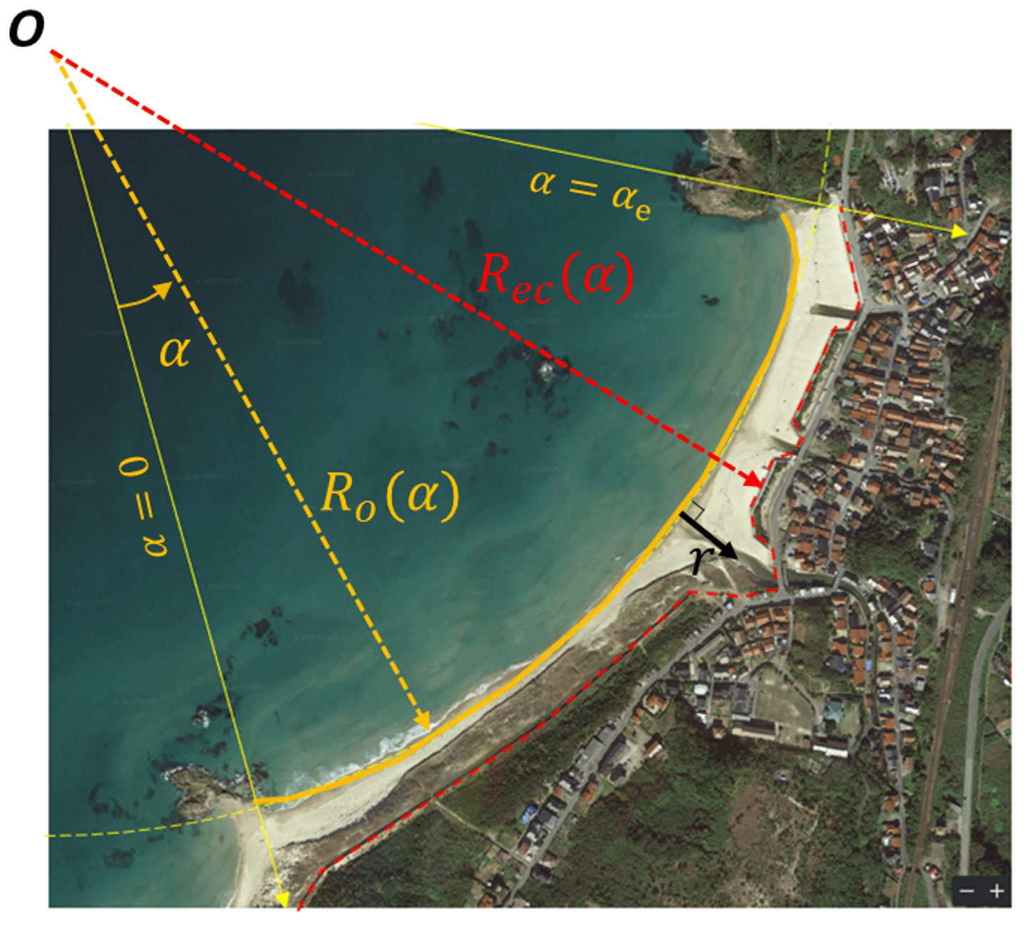
Figure 1Conceptual diagram of combined potential erosion risk (CPER) curve © Google Earth.
Next, the total beach erosion width, Wt, is calculated from the sum of all PEWs obtained from the method described above such that
The right-hand side of Eq. (5) includes the effects of (1) background erosion resulting from a decrease in sediment budget due to watershed development, sand dredging, or extraction, (2) alongshore sediment redistribution and shoreline reshaping due to harbor construction, and (3) short-term erosion due to episodic storms. Because the beach recovers after storm waves, the recoverable episodic erosion (We) will have different values depending on its recurrent interval. When Wt is calculated, as shown in Fig. 2, the overall erosion consequence, Ct can be obtained from a CPERC, which represents the accumulated area likely to be damaged from the EOSL.
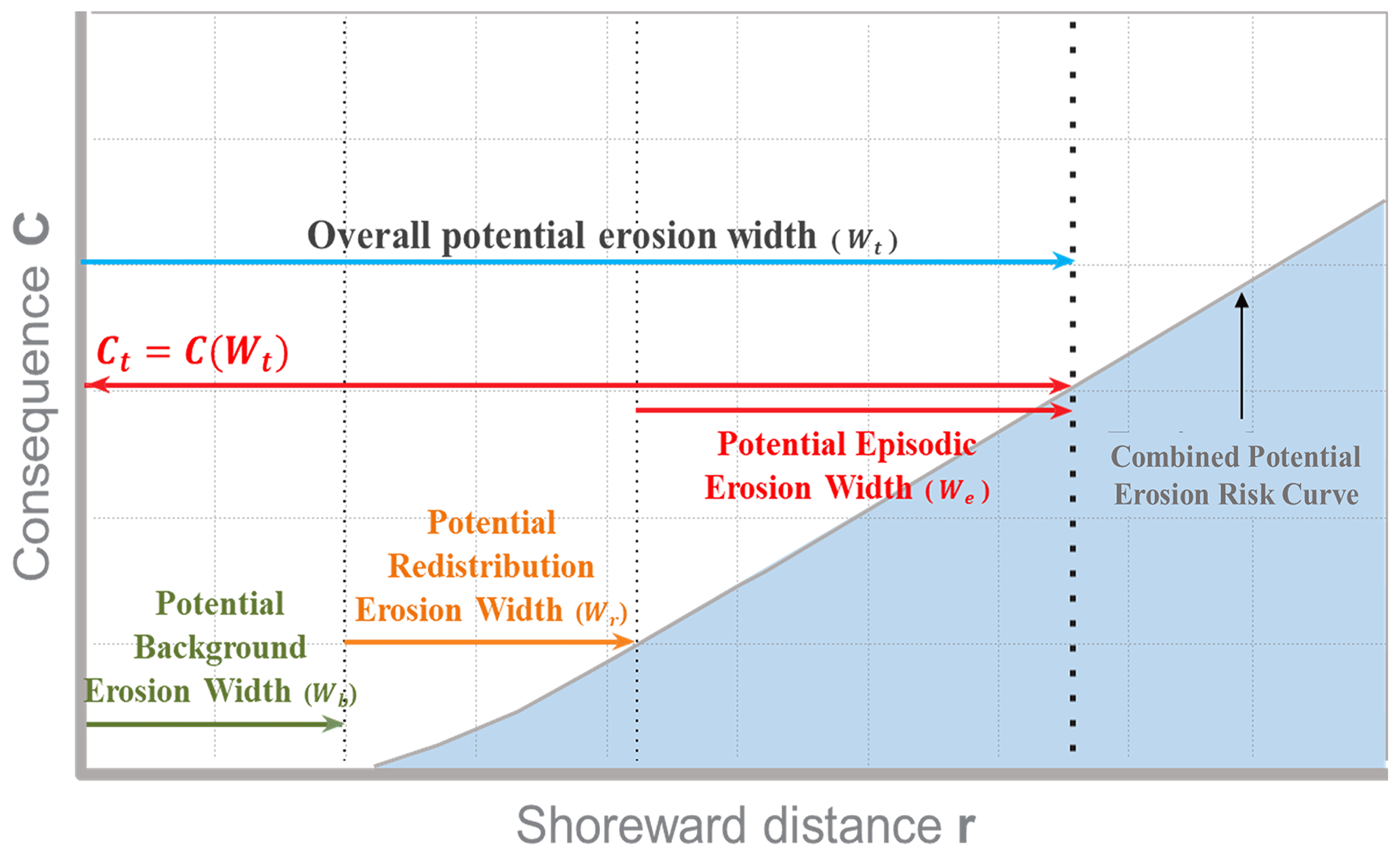
Figure 2Combined potential erosion risk curve (CPERC) constructed from three components of potential erosion width and area.
The abscissa r in Fig. 2 represents the shoreward distance from the average shoreline (EOSL). If the combined potential shoreline retreat, Wt, in Eq. (5) is substituted by r, the CPERC can also represent an area corresponding to consequence C in Eq. (1). To calculate the CPERC area, the frequency related to the background PBEA and PREA can be regarded as one per year (), whereas that for the PEEA (Fe) depends on the frequency of storm occurrence. Therefore, the combined risk R in Eq. (1) can be expressed as follows:
where and , as illustrated graphically in Fig. 2.
3.1 Background erosion from watershed and river (PBEA)
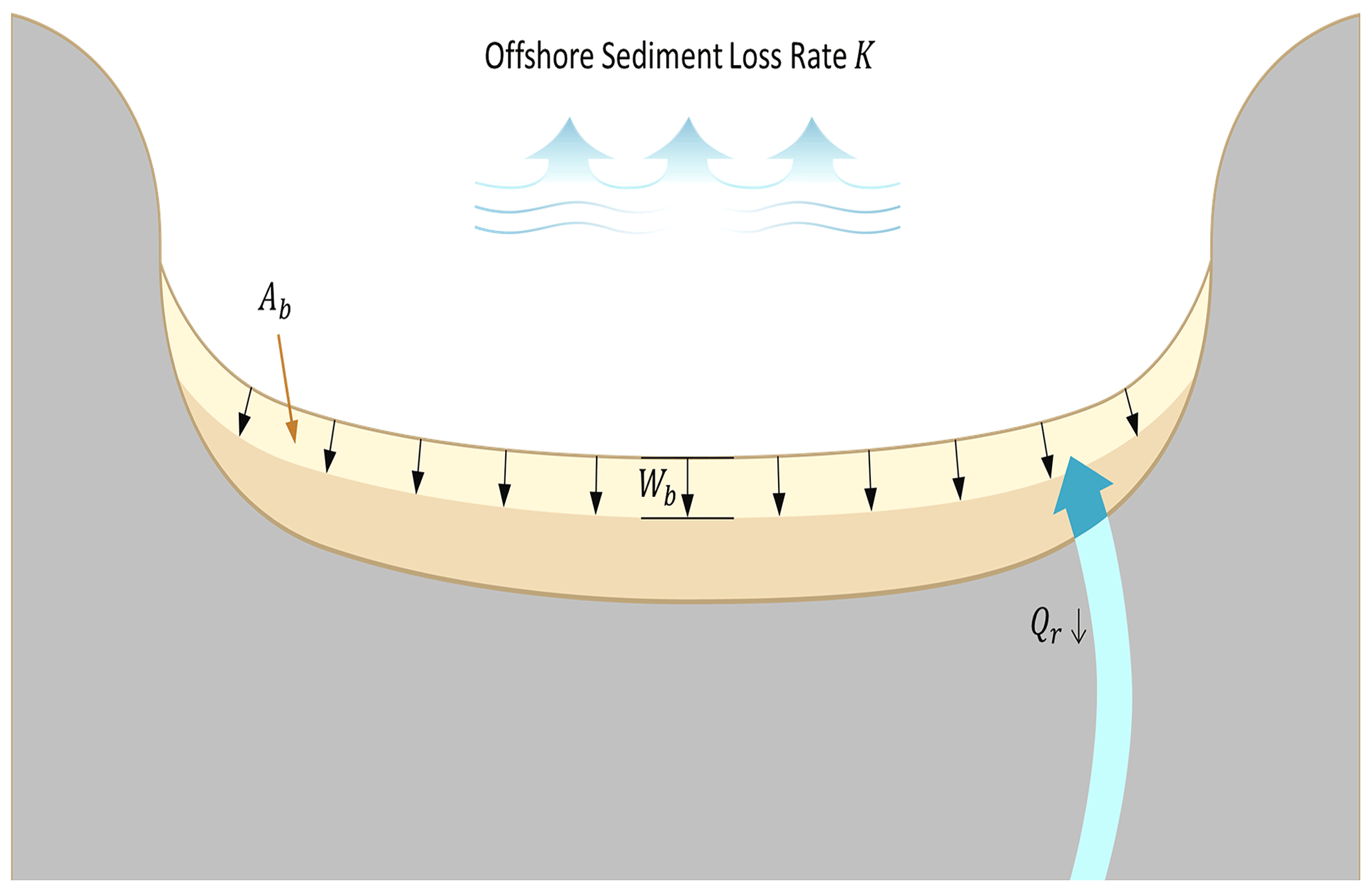
The PBEA (Ab) accounts for beach erosion caused by a decrease in sediment supply from the river. For a sandy beach within a littoral cell (Lee and Lee, 2020), the law of mass conservation gives
where Qin is the ratio of sediment discharge mainly flowing into the littoral cell from a point source such as a river, and Qout is the rate of sediment loss that is steadily lost to the open sea mostly due to the action of waves. However, Qout includes the rate of sand loss due to artificial offshore sand extraction such as sand mining or dredging. In a natural state without artificial coastal zone development, the representative Qin is the sediment discharge rate from the river and is balanced with the loss of sand to the open sea due to the continuous wave action. The latter can be expressed as the product of the sediment loss constant K and the beach sediment volume V (Lee and Lee, 2020).
If the difference between the point source and the sink sediment discharge in the sediment budget, excluding the sand loss to the open sea due to wave action, is defined as ΔQp, the following equation is obtained.
When the amount of sediment in a littoral cell is in equilibrium, the sediment loss constant K can be estimated as ΔQp/V. Here, volume V in the active beach can be approximated as the product of the vertical height of the littoral zone Ds and beach surface area A. Assuming Ds, the sum of berm height and closure depth, is constant along a beach, Eq. (8) becomes
Many studies have been performed to determine the berm height and closure depth, Ds (Rosati, 2005; Cappucci et al., 2011, 2020; Pranzini et al., 2020). Although closure depth varies with wave climate and sediment particle size (Hallermeier, 1981), judging from the observed beach profile data, its value has been shown to remain reasonably constant over several decades.
Because the purpose of this study was to obtain the PBEA, Eq. (9) gives the beach surface area A for a steady state () as follows:
where K and Ds are coefficients representing the characteristics of a beach. Therefore, if ΔQp changes within a coastal environment where K and Ds are constant, the beach surface area will change accordingly. When ΔQp before coastal zone development is set as , and if ΔQp is reduced by , then PBEA (Ab) can be expressed as a function of α as
Here, the superscript “o” corresponds to the beach area before development. Once α is obtained, PBEA can be calculated as described above. However, because of the difficulty in directly determining the α value, additional information is required, such as any changes in land use, forestation, water storage capacity stored by dams, and river maintenance projects in the watershed (Yang and Stall, 1974; Karim and Kennedy, 1990; Wu and Xu, 2006; Slagel and Griggs, 2008; Gunawan et al., 2019).
Assuming Ab is uniformly distributed over the entire embayment with a curved length Lb, then the PBEW as shown in Fig. 3.
3.2 Reshaping of shoreline due to harbor breakwater (PREA)
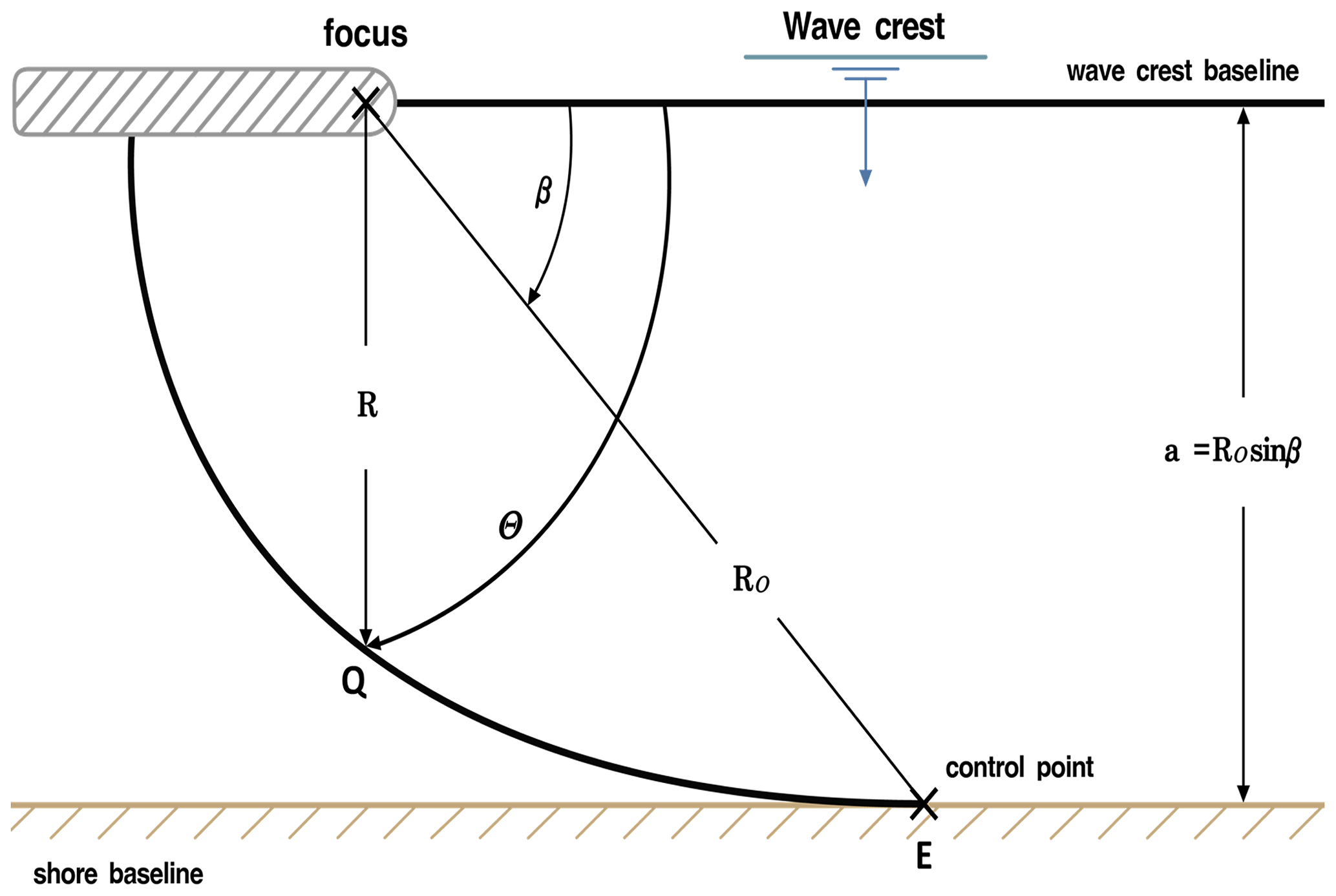
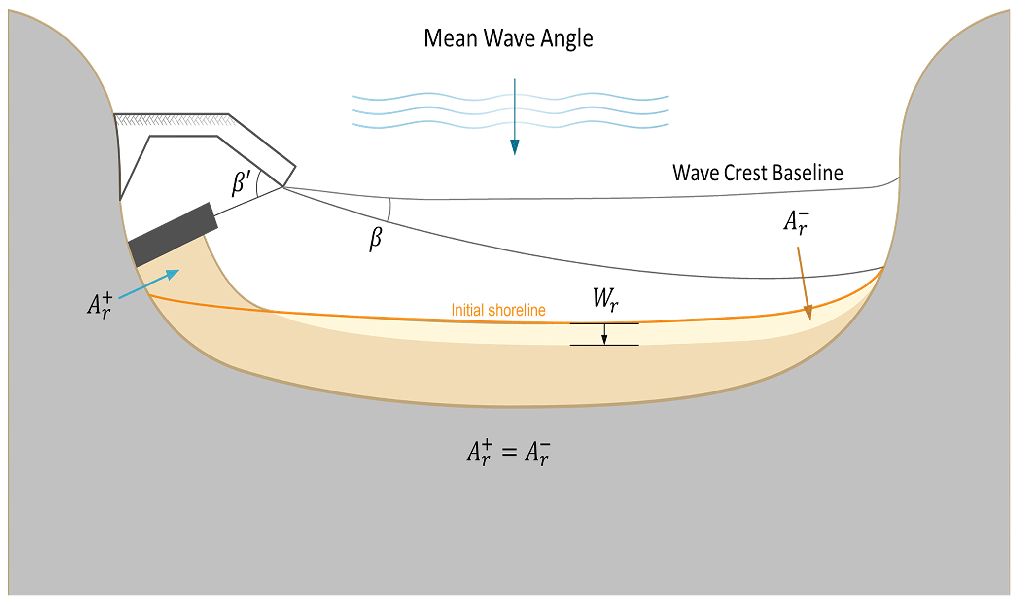
Harbor construction on sandy coasts often changes the wave field, generating new wave diffraction and nearshore current patterns. It also causes “shoreline reshaping”, with downdrift erosion accompanied by updrift accretion. Although the amount of sediment may be maintained within a cell, the erosion risk area (called PREA) induced by the redistribution of littoral drift can be assessed by an empirical parabolic shoreline model of parabolic type (i.e., PBSE; Hsu and Evans, 1989). This model can be readily applied to predict the static bay shape on a downdrift beach with the breakwater tip as a control point. This equation (in polar coordinates) can be used to define two adjoining regions with a common tangent at the downdrift control point E (Fig. 4):
where R0 is the length of the control line (FE) joining the parabolic focus (F; wave diffraction point) and the downdrift control point E, R(θ) is the radius from the focus to a point Q on the equilibrium shoreline, a is the perpendicular distance from the wave crest baseline to point E, β is the angle between the wave crest baseline and the line joining the focus and the control point, θ is the angle between the wave crest baseline and the line connecting F and Q, and C0, C1, and C2 are the coefficients provided by Hsu and Evans (1989). An approximate expression for the PBSE is given by
Recently, Lim et al. (2021) extended the applicability of the PBSE with polar coordinates to concave coasts. In the present case, the actual equilibrium shoreline can be estimated by shifting the downdrift segment of the predicted bay shape landward, parallel to the existing shoreline, and equating the accreted area with the eroded area , as shown in Fig. 5. The accreted area, which is the PREA, can also be derived from Eq. (13), rendering
In Eq. (14) and Fig. 5, β′ is the angle between the focus point (i.e., the breakwater tip) and the secondary breakwater. For application, Eq. (14) can be approximated as follows:
Then, PREW Wr can be calculated by dividing the accretion area Ar by Lr, which is the length from the focus point to the farthest point on the downdrift beach or the shoreline length in the erosion section (Fig. 5).
3.3 Episodic storm caused beach erosion (PEEA)
The PEEA is defined as a beach surface that is temporarily eroded by storms. However, it is also characterized by a gradual return of the beach profile to the original shoreline after the storm wanes. Figure 6 shows the variation in the mean beach profile with a near-constant depth of closure at Bongpo–Cheonjin Beach. This reveals that the statistical distribution of shoreline survey data collected four times each year follows a normal distribution. Although these surveys are intended to present seasonal changes in shoreline variability, they are unlikely to reflect short-term changes during storms; if a series of survey data is sufficient for including storm effect, the daily extreme value can be calculated by multiplying the probabilistic analysis results by a weighting factor of 1.5. The validity of this method was verified by applying Tairua Beach in New Zealand (Montaño et al., 2020), which has sampling data for more than 8 years.

Figure 6Variation in beach profile and shoreline position and the probability distribution (inset) at a beach in South Korea.
When the observed shoreline data follow a normal distribution, it can be applied to assess the maximum probable erosion occurring once in n years with a probability of in a cumulative normal distribution curve, from which the frequency F for a shoreline variable xF can be estimated by
From Eq. (16), the shoreline position due to episodic erosion Se is then calculated for a shoreline variation width xF by
where μ is the mean position of the shoreline, and σ is the standard deviation of the shoreline variation width obtained from the data distribution curve. The PEEW with a certain return period can then be estimated statistically from the shoreline observation data such that
where the frequency F(xF) corresponds to the frequency Fe in the potential erosion risk given in Eq. (6). However, since the shoreline was observed four times a year, it was approximated by multiplying by 1.5 to convert it into a daily statistical value of the variation for a 30-year return period (e.g., ).
Finally, PEEA (Ae) is obtained by multiplying PEEW (We) by its effective shoreline length Le. The proposed method cannot be applied because there are no shoreline survey data or the amount of data is insufficient for statistical analysis. The PEEW can be estimated using an equilibrium beach profile (Dean, 1977) from storm wave and sediment particle size data (Kim and Lee, 2018).
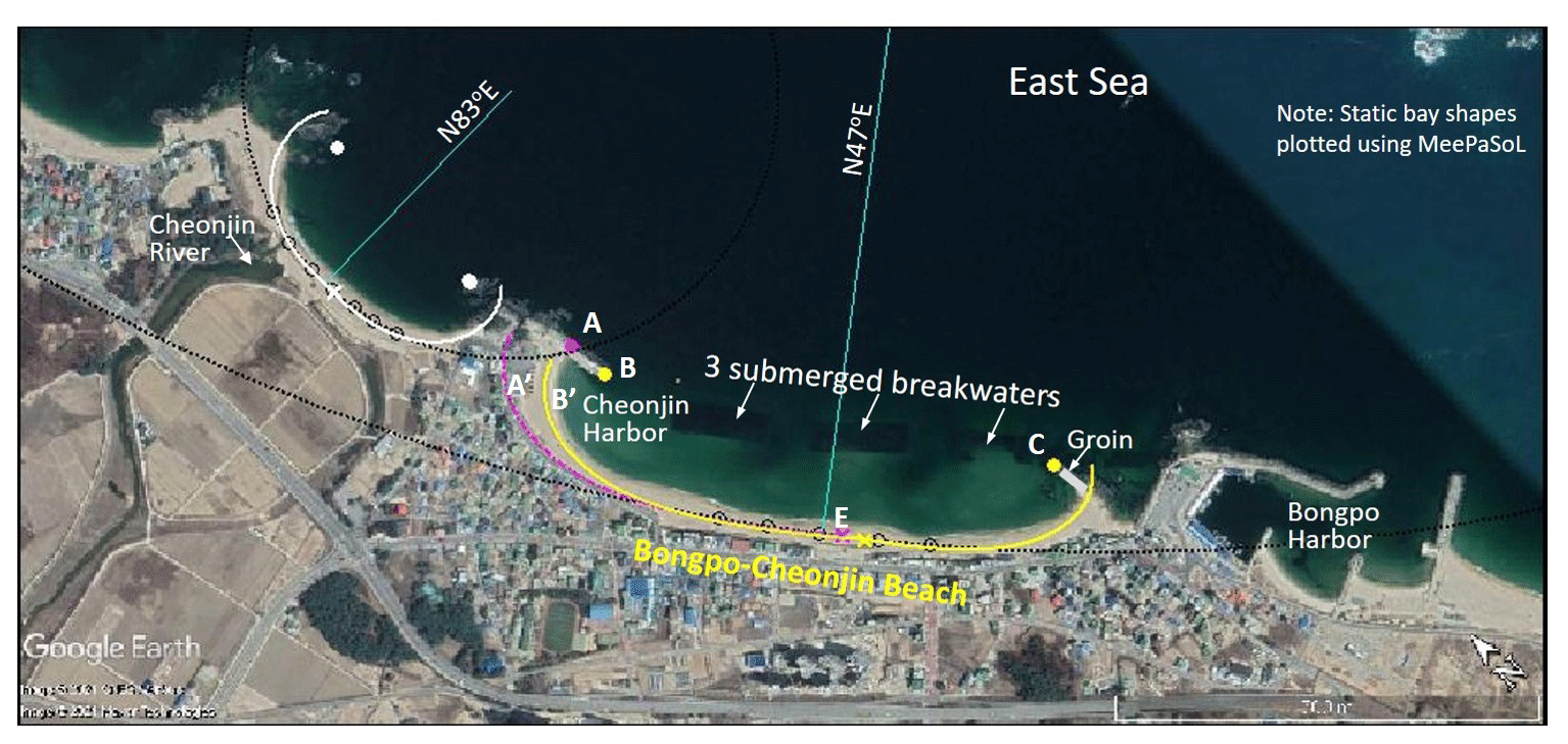
Figure 7Aerial photograph of Bongpo–Cheonjin Beach in February 2021, showing harbors, river, shore protection structures, and static bay shapes, produced by the software MeePaSoL © Google Earth.
4.1 Site description
The quantitative assessment proposed in the present study was applied to Bongpo–Cheonjin Beach (38∘15′ N, 128∘33′ E), in the northeast of Gangwon-do (province), South Korea, where the small Cheonjin Harbor is located to the north and the large Bongpo Harbor to its south (Fig. 7). The beach is of a crenulated shape, approximately 1.1 km long, and is a closed littoral cell due to the existence of the breakwater (completed in November 2010) for Cheonjin Harbor in the updrift region and a group of natural rocks nearshore in the downdrift region. Because beach erosion often occurs due to increased swell and larger waves in winter, three segmented submerged breakwaters totaling 490 m in length (installed between November 2017 and November 2019) and one groin of 40 m (completed in July 2018) extending out from the rocks eventually transformed the beach into a stable embayment (Fig. 7).
The application of the software MeePaSoL (Lee, 2015) developed for the PBSE (Hsu and Evans, 1989) revealed that Bongpo–Cheonjin Beach is currently close to static equilibrium (using focus points B and C for the updrift and downdrift half of the beach shown in the yellow curve, respectively; Fig. 7).
In geomorphic terms, Bongpo–Cheonjin Beach has received predominant waves from approximately the 47∘ E direction (drawn by software MeePaSoL), whereas the prevailing wave direction in spring and summer is from 50∘ E and in autumn and winter from 30∘ E in the open sea. Therefore, longshore sediment transport prevails from north to south in autumn and winter, especially during periods of high wave action in winter, which has caused severe beach erosion.
4.2 PBEA due to development in watershed
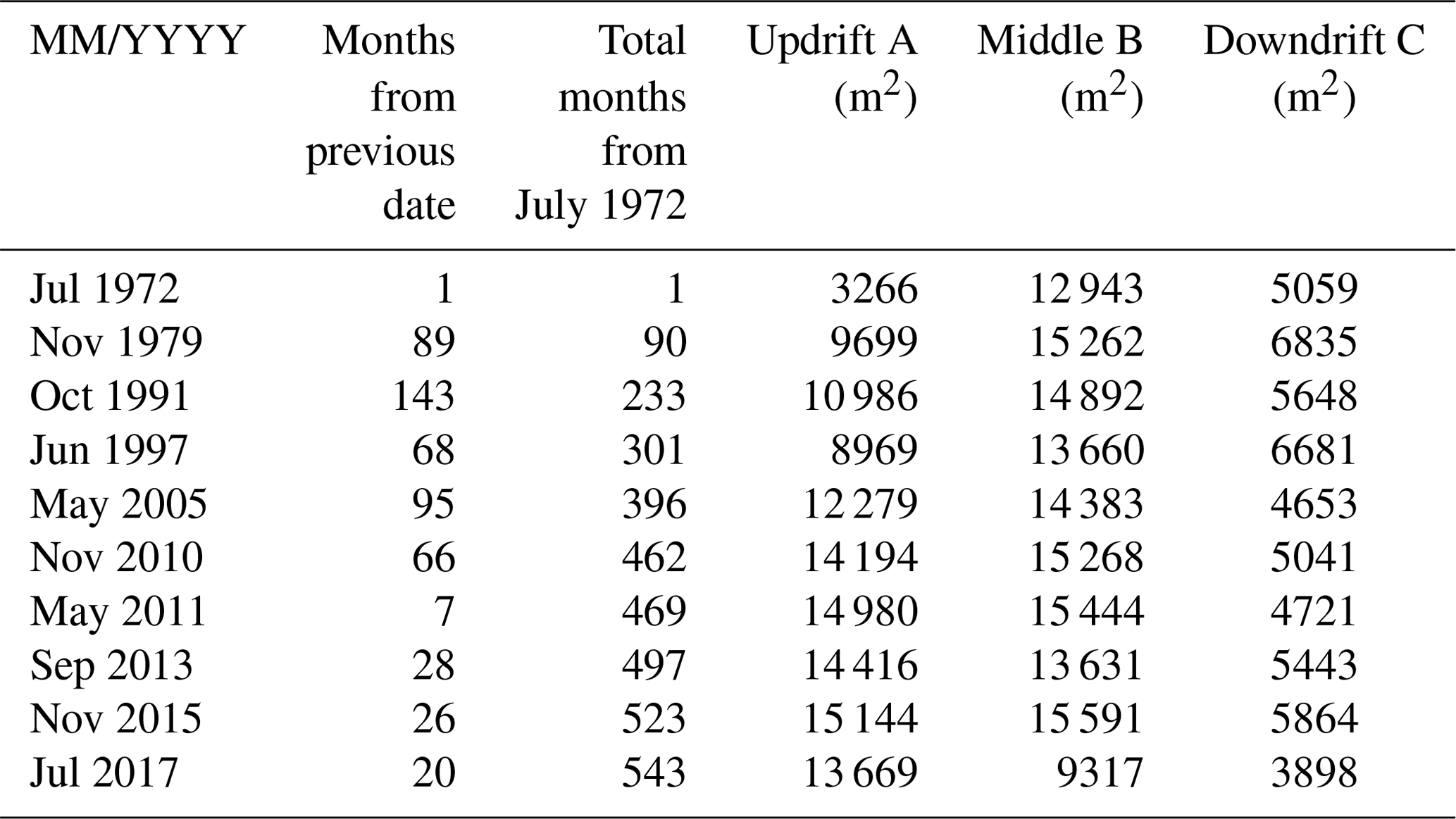
The Cheonjin River watershed, which contains three rivers and covers an area of 69.51 km2 is linked to the littoral cell at Bongpo–Cheonjin Beach. Although a series of developments in the watershed (e.g., construction of several small weirs, change in forest environment, and river maintenance projects) have had the potential to reduce the sediment input to the beach, its impact on the background PBEA and PBEW was found to be minimal upon analyzing a series of 10 aerial photographs of Bongpo–Cheonjin Beach (Fig. 8) spanning over 45 years from 1972 to 2017 (i.e., July 1972, November 1979, October 1991, June 1997, May 2005, November 2010, May 2011, September 2013, November 2015, and July 2017). The values of shoreline position, beach width, and beach area were extracted from three key locations (A, B, and C marked on each sub-panel in Fig. 8) and tabulated in Table 1. In addition, 37 sets of seasonal shoreline survey data collected during 2008–2017 and NOAA's wave data were also utilized, and the results are presented graphically in Fig. 9.

Figure 8Aerial photographs of Bongpo–Cheonjin Beach by year: (a) July 1972, (b) November 1979, (c) October 1991, (d) June 1997, (e) May 2005, (f) November 2010, (g) May 2011, (h) September 2013, (i) November 2015, and (j) July 2017. Images courtesy of the National Geographic Information Institute (The Province of Gangwon, 2018).
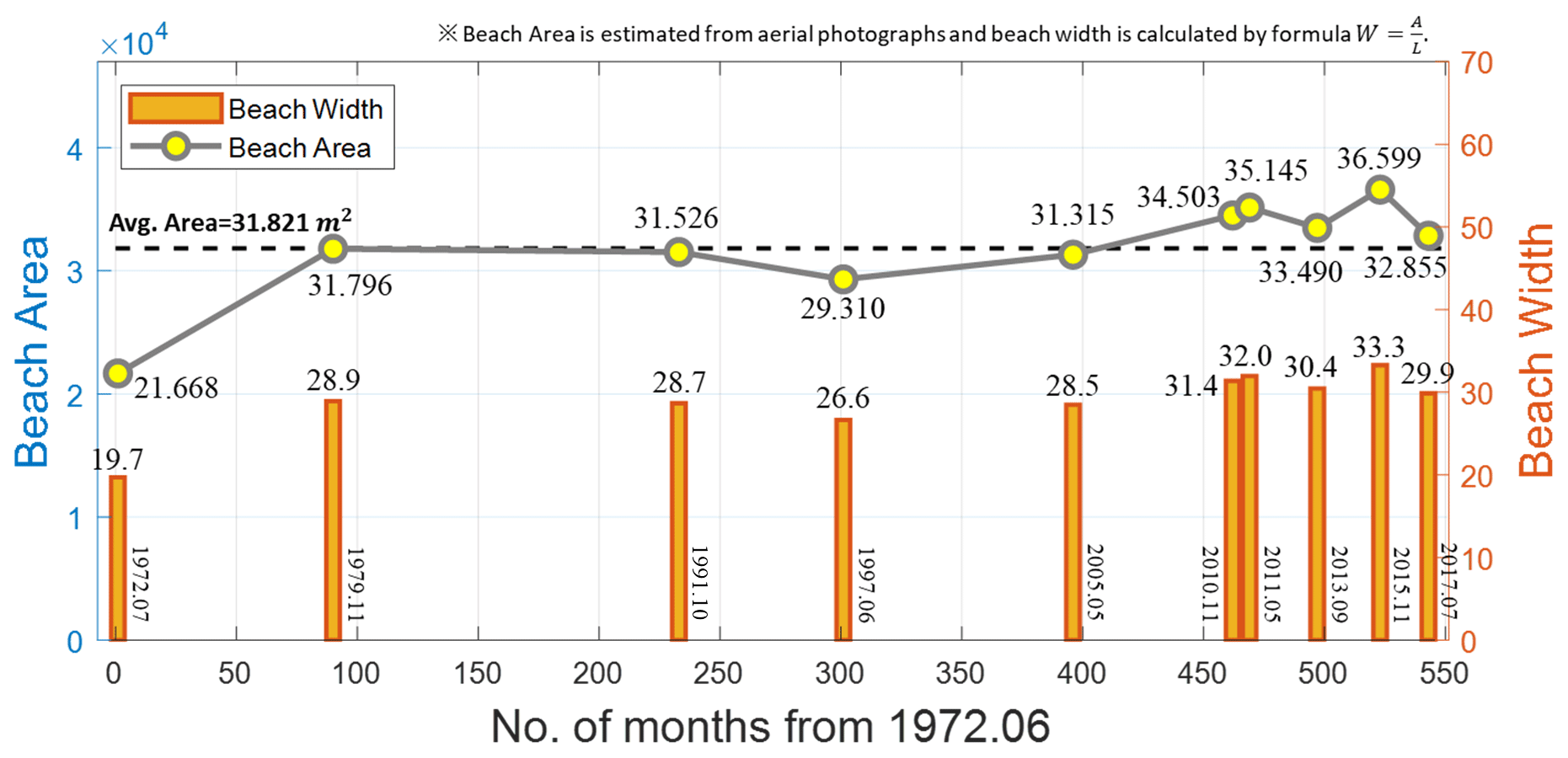
Figure 9Variations in beach area and width for Bongpo–Cheonjin Beach using aerial photographs.
From each aerial photograph, the average beach width was obtained by dividing the beach area by the shoreline length at the time of photographing. Therefore, depending on the incident wave conditions at that time, it may not be able to reflect the effect of shoreline retreat caused by cross-shore sediment transport. Nonetheless, statistical analysis indicates that the erosion width occurring at a frequency of 1 year is approximately 16 m at the Bongpo–Cheonjin Beach.
As shown in Fig. 9, since November 1979, total beach area at Bongpo–Cheonjin has remained around 31 800 m2, about the average of 31 821 m2, or higher after May 2005, except between November 1991 and May 2005, whereas beach width has maintained about 28 m or more, except in June 1997 when it was reduced to 26.6 m. Although small submerged weirs were built along Cheonjin River, its effect on the background sediment budget Ab is minimal due to the small storage capacity of the weirs. Since the estuary of the Cheonjin River is located outside the Bongpo–Cheonjin Beach, it is not expected to significantly influence on PBEW depending on the potential bypass of sediment from the beach at the north. Therefore, considering the net effect of all agents, at the decadal scale, the Bongpo–Cheonjin Beach can be considered (more or less) to be in equilibrium. Hence, the PBEW Wb may be ignored in this study.
4.3 PREA due to the construction of harbor breakwater
As shown in Fig. 9, the averaged beach width of the Bongpo–Cheonjin Beach appears to have remained at approximately 30 m for a long time after mid 2008 (by linear interpolation between May 2005 and November 2010) in spite of the regional shoreline advancing to form a static bay shape after the construction of the Cheonjin Harbor breakwater. During this period, shoreline reshaping resulted in sediment deposition in the vicinity of the breakwater (at updrift A) and accompanying erosion (at downdrift C) of the beach, as shown in Table 1.
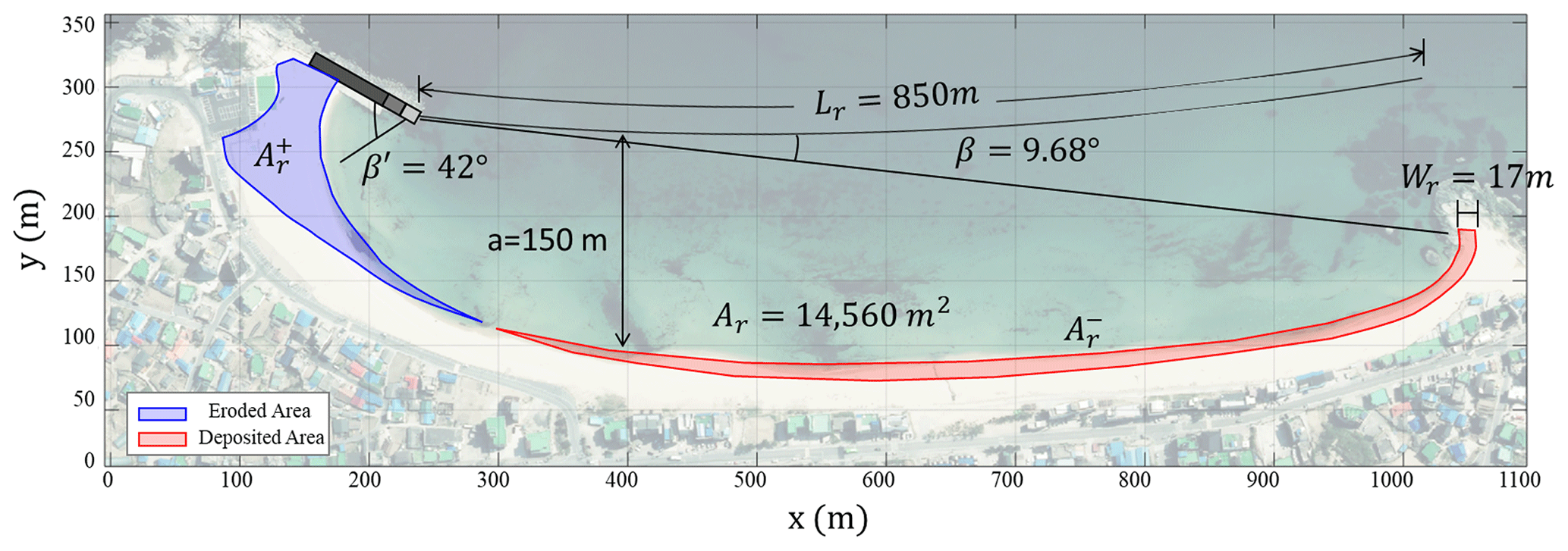
Figure 10Calculation of PREA at Bongpo–Cheonjin Beach. Image courtesy of the National Geographic Information Institute (MOF, 2020).
Table 1Variations in beach area at three key locations of Bongpo–Cheonjin Beach marked in Fig. 8 (The Province of Gangwon, 2018).
The PREA can be approximated by the bay-shaped shoreline feature across the entire Bongpo–Cheonjin Beach (Fig. 10). First, the equivalent wave obliquity (β) from the tip of the harbor breakwater can be approximated from the geometry of indentation (a) in relation to the beach length (Lr):
PREA Ar is then obtained by substituting the calculated β with β′, as indicated in Fig. 5 and Eq. (15):
For a=150 m (Fig. 10), Eq. (20) gives Ar=14 560 m2. The relationship between β and β′ in Eq. (15) can be plotted (Fig. 11) to obtain the dimensionless PREA () with values from 0 to 10. Alternatively, the value for can be obtained graphically, as shown in Fig. 11. By equating with (Fig. 10), the beach erosion width Wr was estimated to be 17 m by inputting the beach length from the breakwater (Lr=850 m) into Eq. (2).

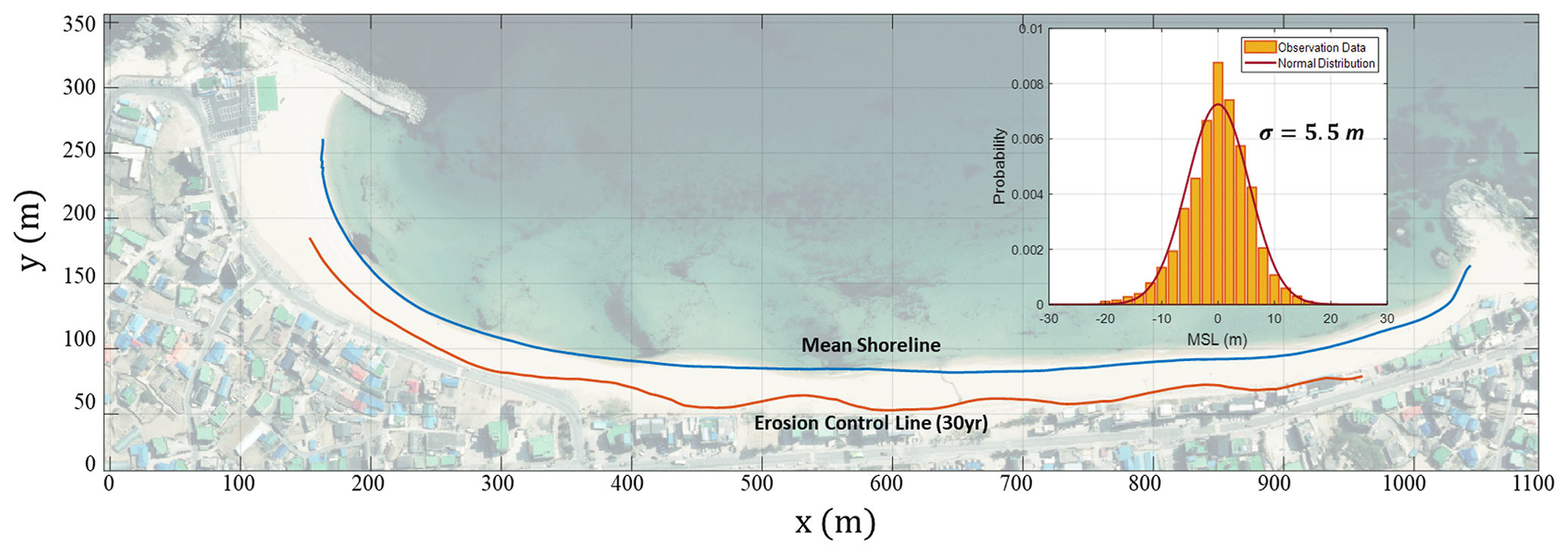
Figure 12PEEA at Bongpo–Cheonjin Beach, showing standard deviation σ and mean encroachment σxF with a 30-year return period (within inset). Image courtesy of the National Geographic Information Institute (MOF, 2020).
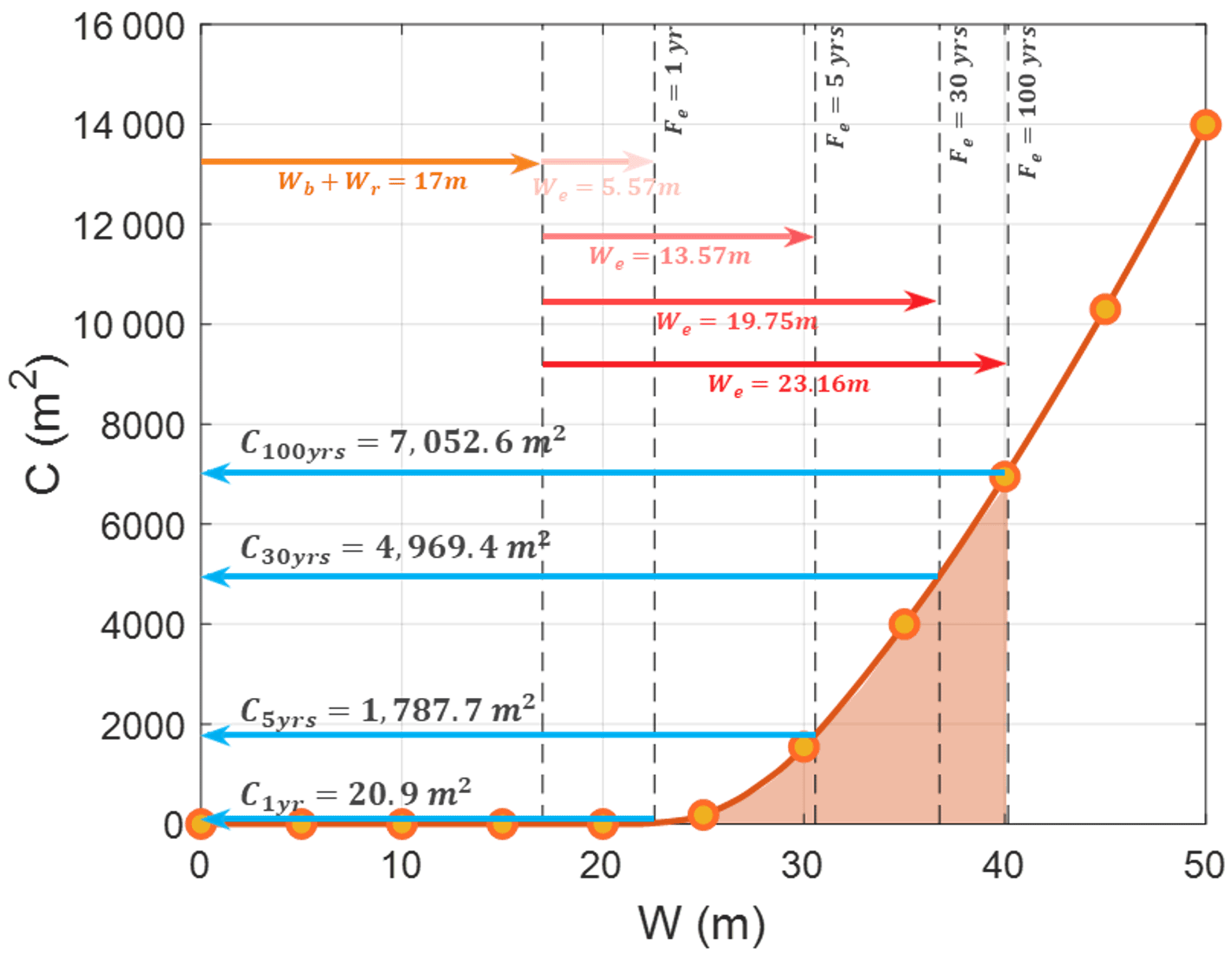
Figure 13Estimation of combined potential erosion risk using the CPERC for Bongpo–Cheonjin Beach.
4.4 PEEA due to episodic storm
Routine shoreline surveys have been conducted at least four times per annum for beaches in Gangwon-do, South Korea, since the 2000s. More specifically, a total of 37 sets of seasonal data were collected over 10 years from 2008 to 2017 for the Bongpo–Cheonjin Beach. These data were plotted and fitted by a normal distribution (Fig. 12) to show local shoreline changes with a standard deviation of σ=5.5 m. Figure 12 also compares the alongshore distribution of the mean shoreline and eroded shoreline of the 30-year return period from statistical analyses (xF=3.6). The beach width due to the PEEW is evaluated as the value with the range from 5.57 to 23.16 m ().
4.5 CPER curve for Bongpo–Cheonjin Beach
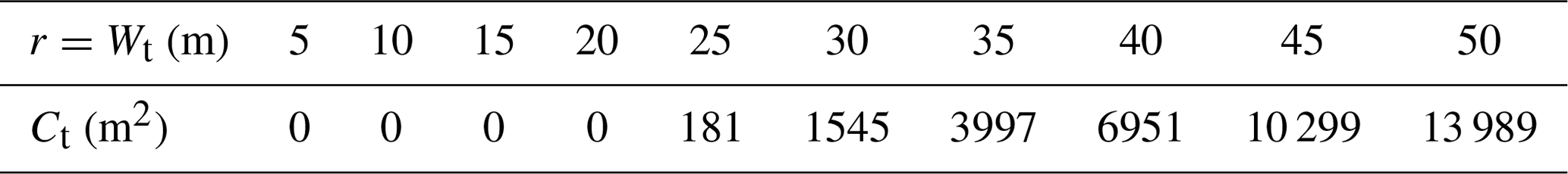
The potential erosion risk to a beach can be obtained by accumulating all the erosion risk widths from each contributing factor, resulting in a CPERC (Sect. 2.3 and Fig. 2). In Fig. 13, the CPERC accounts for the erosion risk distance from the EOSL. At Bongpo–Cheonjin Beach, the PBEW Wb and PREW Wr are estimated to be 0 and 17 m, respectively, thus representing the sum of the first two individual components m. Furthermore, by calculating the combined erosion risk width Wt (Eq. 5) at 5 m intervals, up to 50 m, the corresponding values for consequence Ct are tabulated as in Table 2.
Table 2Relationship between combined shoreline retreat Wt and consequence Ct for Bongpo–Cheonjin Beach.
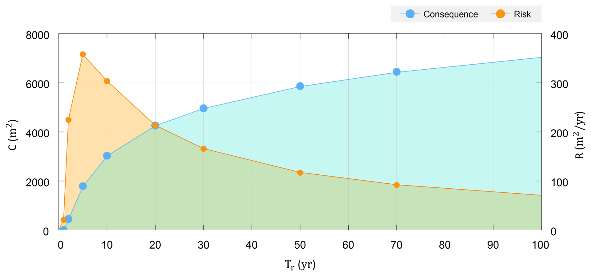
Because PEEW We is a function of the return period (frequency) of storm occurrence, the total shoreline retreat (Wt), consequence (Ct), and erosion risk (R; Eqs. 1 and 6) are calculated for several specific return periods (in years) of storms, as shown in Table 3. In addition, Fig. 13 illustrates the consequence Ct per return period , which is obtained using the CPERC, while Fig. 14 shows the variation in consequence and the combined potential erosion risk with respect to the storm return period at Bongpo–Cheonjin Beach.
Table 3Potential erosion risk per return period Tr for Bongpo–Cheonjin Beach using CPERC.
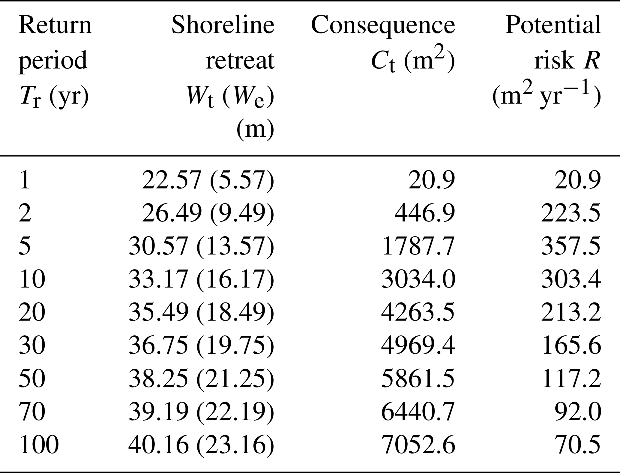
Overall, from the analysis of potential beach erosion area and width for the three key factors at Bongpo–Cheonjin Beach, the PBEW may be considered insignificant; hence, Wb≈0, but PREW (Wr) is estimated to be 17 m following a 40 m extension to the breakwater for Cheonjin Harbor. In addition, the PEEW (We) value is estimated to be between 5.57 and 19.75 m for the storm return period (Fe) of 1 and 30 years, respectively. Upon applying the combined shoreline retreat () to the CPERC, it yields the total eroded beach area ranging from 20.9 to 4969.4 m2 (see Fig. 13 and Table 3). For a storm with a 30-year return period, this implies that a beach area totaling 4969.4 m2 (or beach width of approximately 36.75 m) might be eroded once every 30 years, thus requiring appropriate engineering solutions (such as coastal setbacks, beach nourishment, or others) to conserve the coastal environment at Bongpo–Cheonjin Beach.
The limitations of the assessment method proposed in this study are briefly described, together with additional considerations, to enhance the applicability of this methodology to different coastal environments.
-
Although the purpose of this study is to apply an assessment method to Bongpo–Cheonjin Beach, which is a shallow embayment or a semi-closed littoral cell, the proposed method is not limited to headland–bay beaches. It is also applicable to open beaches with suitable modifications to the mechanisms examined in this study.
-
The proposed combined potential erosion risk curve (CPERC) includes an individual risk component assessed for background sediment from a river at updrift, a fishing harbor with breakwater extension, and storm waves in winter. The construction of CPERC is based on a simple arithmetic sum to represent the worst case scenario rather than a multivariable regression analysis. It cannot predict temporal changes in erosion risk. To improve the reliability of this method, the temporal beach change and the scale of each contributing factor versus time must be examined, especially from that induced by the episodic storm that occurs only sporadically. Conversely, the other two are either almost constant or increasing gradually.
-
For Bongpo–Cheonjin Beach, the potential background erosion width (PBEW, Wb) is negligible, indicating that the variation in sediment supply from the watershed is minimal. However, after a large dam is constructed within a watershed, the time-dependent change in beach width must be considered. The theoretical solution given by Lee and Lee (2020) suggests the effects of the sand loss rate Kb into the open sea, and the decrease rate α of the sediment supply to the beach can be expressed as
where α and Kb are constant, and the corresponding beach area is assumed to converge to (1−α)Ao, where Ao is the initial area. Equation (21) shows that the beach area decreases rapidly at the beginning but converges to 95 % or more of the equilibrium state when t is greater than years.
-
To increase the accuracy of potential erosion width (PREW, Wr) due to shoreline reshaping caused by breakwater construction for harbors, empirical formulae (e.g., the CERC, 1984, equation in the Shore Protection Manual) can be applied. Starting from the angle difference between the initial and equilibrium shoreline angles at the boundary of erosion and deposition, the temporal width change was obtained by applying an exponentially converging angle change to the formula for longshore sediment transport:
where is the ultimate beach width due to longshore sediment transport, and Kr is the rate of change in angle according to the time at the junction, which is estimated by dividing the longshore sediment transport rate by the beach length Lr and the vertical littoral height Ds in the formula for longshore sediment transport. The equilibrium shoreline angle due to harbor or coastal structures can be obtained based on the PBSE of Hsu and Evans (1989).
-
For potential beach erosion due to episodic storms (PEEW, We) that can be recovered after the storm wanes, Yates et al. (2009) have confirmed that a linear relationship exists between the location of the shoreline and swell wave energy in field observations. Applying this recoverable process, the shoreline change model proposed by Miller and Dean (2004) can be expressed by the ordinary differential equation (Kim, 2021),
where Kb is the beach recovery factor, Eb is the wave energy at the breaking point, and a is the beach response factor between the wave energy Eb and the mean shoreline. When the value of Ke, which is unique for each beach, is known, the temporal change in the shoreline can be estimated from Eq. (23) for a given wave energy. Alternatively, the SBEACH model may be used (Larson and Kraus, 1989; Larson et al., 1990).
This study presents a quantitative method for assessing the potential erosion area (PEA) and potential erosion width (PEW) due to development in the watershed, harbor construction, and storm impact. Aerial photographs, beach surveys, and NOAA wave data were applied to support the analysis while omitting sea-level rise. The results are used to produce a combined potential erosion risk curve (CPERC) for planning coastal protection or restoration projects which include the effectiveness of potential risk induced by storms in different return periods of occurrence. For example, the potential erosion risk due to storms (PEEW, We) over a 30-year return period is estimated to be about 19.75 m (Table 3), which gives a total potential erosion risk width (Wt) of 36.75 m. This is greater than the beach width of 30 m from the current averaged shoreline (EOSL), thus calling for engineering solutions to protect Bongpo–Cheonjin Beach. Because of the potential severity of the predicted beach erosion risk, for beach nourishment three submerged detached breakwaters (each 160 m long with a gap of 70 m) were constructed from November 2017 to November 2019, with a short groin (40 m) (Fig. 7). These have satisfactorily transformed Bongpo–Cheonjin Beach into a stable embayment since the completion of the engineering work.
By applying the risk assessment method presented in this paper, it is possible to determine the optimal strategy by comparing the total cost of risk to the eroding section with the average annual cost of erosion protection. Moreover, the proposed methodology is helpful not only for quantitatively assessing beach erosion risk but also for devising engineering countermeasures to mitigate the causes of erosion. Further research is recommended to apply the methodology described in this paper to beaches suffering severe erosion so that this method can be improved and benefit other coastal communities through its application.
No data sets were used in this article.
CL and JLL conceived the idea. CL, TKK, SL, and YJY participated in the field data collection. CL, SL, and JLL participated in data interpretation. All authors contributed to the writing of the final draft.
The contact author has declared that neither they nor their co-authors have any competing interests.
Publisher's note: Copernicus Publications remains neutral with regard to jurisdictional claims in published maps and institutional affiliations.
This research was part of the “Practical Technologies for Coastal Erosion Control and Countermeasure” project supported by the Ministry of Oceans and Fisheries, South Korea (grant no. 20180404).
This paper was edited by Daniele Giordan and reviewed by two anonymous referees.
Ab Razak, M. S., Jamaluddin, N., and Mohd Nor, N. A. Z.: The platform stability of embayed beaches on the west coast of Peninsular Malaysia, Jurnal Teknologi, 80, 33–42, 2018a.
Ab Razak, M. S., Mohd Nor, N. A. Z., and Jamaluddin, N.: Platform stability of embayed beaches on the east coast of Peninsular Malaysia, Jurnal Teknologi, 13, 435–448, 2018b.
Anh, D. T. K., Stive, M. J. F., Brouwer, R. L., and de Vries, S.: Analysis of embayed beach platform stability in Danang, Vietnam, in: Proceedings of the 36th IAHR World Congress, 28 June–3 July 2015, the Hague, the Netherlands, 2015.
Ballesteros, C., Jiménez, J. A., Valdemoro, H. I., and Bosom, E.: Erosion consequences on beach functions along the Maresme coast (NW Mediterranean, Spain), Nat. Hazards, 90, 173–195, 2018.
Bayram, A., Larson, M., and Hanson. H.: A new formula for the total longshore sediment transport rate, Coast. Eng., 54, 700–710, 2007.
Beven II, J. L., Avila, L. A., Blake, E. S., Brown, D. P., Franklin, J. L., Knabb, R. D., Pasch, R. J., Rhome, J. R., and Stewart, S. R.: Atlantic Hurricane Season of 2005, Mon. Weather Rev., 136, 1109–1173, https://doi.org/10.1175/2007MWR2074.1, 2008.
Bowman, D., Guillén, J., López, L., and Pellegrino, V.: Planview geometry and morphological characteristics of pocket beaches on the Catalan coast (Spain), Geomorphology, 108, 191–199, 2009.
Bray, M. J., Carter, D. J., and Hooke, J. M.: Littoral cell definition and budgets for central southern England, J. Coast. Res., 11, 381–400, 1995.
Callaghan, D. P., Ranasinghe, R., Nielsen, P., Larson, M., and Short, A. D.: Process-determined coastal erosion hazards, in: Proceedings of the 31st International Conference on Coastal Engineering, World Scientific, Hamburg, Germany, 4227–4236, 2008.
Cappucci, S., Scarcella, D., Rossi, L., and Taramelli, A.: Integrated Coastal Zone Management at Marina di Carrara Harbor: Sediment management and policy making, J. Ocean Coast. Manage., 54, 277–289, 2011.
Cappucci, S., Bertoni, D., Cipriani, L. E., Boninsegni, G., and Sarti, G.: Assessment of the Anthropogenic Sediment Budget of a Littoral Cell System (Northern Tuscany, Italy), Water, 12, 3240, https://doi.org/10.3390/w12113240, 2020.
Casas-Prat, M. and Sierra, J. P.: Trend analysis of wave direction and associated impacts on the Catalan coast, Climatic Change, 115, 667–691, https://doi.org/10.1007/s10584-012-0466-9, 2012.
CERC – Coastal Engineering Research Center: Shore Protection Manual, 4th Edn., US Army Corps of Engineers, Waterways Experiment Station, Coastal Engineering Research Center, US Government Printing Office, Washington, DC, 1984.
Cooper, N. J.: Engineering Performance and Geomorphic Impacts of Shoreline Management at Contrasting Sites in Southern England, PhD Thesis, University of Portsmouth, Hampshire, England, 1997.
Cooper, N. J. and Pethick, J. S.: Sediment budget approach to addressing coastal erosion problems in St. Oueen's Bay, Jersey, Channel Island, J. Coast. Res., 21, 112–122, 2005.
Dean, R. G.: Equilibrium beach profiles: U.S. Atlantic and Gulf Coasts, Technical Report No. 12, Department of Civil Engineering, University of Delaware, Delaware, 1977.
Dolan, T. J., Castens, P. G., Sonu, C. J., and Egense, A. K.: Review of sediment budget methodology: ocean side littoral cell, California, in: Proceedings of Coastal Sediments '87, ASCE, 12–14 May 1987, New Orleans, USA, 1289–1304, 1987.
Edward, B. T., Abby, S., Juan, C. S., Laura, E., Timothy, M., and Rost, P.: Sand mining impacts on long-term dune erosion in southern Monterey Bay, Mar. Geol., 229, 45–58, 2006.
Foley, M. M., Jonathan, A. W., Andrew, R., Andrew, W. S., Patrick, B. S., Jeffrey, J. D., Matthew, M. B., Rebecca, P., Guy, G., and Randal, M.: Coastal habitat and biological community response to dam removal on the Elwha River, Ecol. Monogr., 87, 552–577, 2017.
González, M., Medina, R., and Losada, M. A.: On the design of beach nourishment projects using static equilibrium concepts: Application to Spanish coast, Coast. Eng., 57, 227–240, 2010.
Gunawan, T. A., Daud, A., and Sarino: The Estimation of Total Sediments Load in River Tributary for Sustainable Resources Management, IOP Conf. Ser.: Earth Environ. Sci., 248, 012079, https://doi.org/10.1088/1755-1315/248/1/012079, 2019.
Hallermeier, R. J.: A profile zonation for seasonal sand beaches from wave climate, Coast. Eng., 4, 253–277, 1981.
Hansson, S. O.: Risk, The Stanford Encyclopedia of Philosophy, in: Summer 2007 Edition, edited by: Zalta, E. N., Metaphysics Research Lab, Stanford University, available at: https://plato.stanford.edu/archives/fall2018/entries/risk/ (last access: 17 December 2021), 2007.
Harley, M., Armaroli, C., and Ciavola, P.: Evaluation of XBeach predictions for a real-time warning system in Emilia-Romagna, Northern Italy, J. Coast. Res., 64, 1861–1865, 2011.
Herrington, S. P., Li, B., and Brooks, S.: Static equilibrium bays in coast protection, Marine Engineering Group, Institution of Civil Engineers, London, UK, 2007.
Hsu, J. R. C. and Evans, C.: Parabolic bay shapes and applications, in: Proceedings of Institution of Civil Engineers, Part 2, Vol. 87, Thomas Telford, London, 557–570, 1989.
Hubbard, D. W.: The Failure of Management: Why It's Broken and How to Fix It, John Wiley & Sons, Hoboken, 2009.
Inman, D. L. and Jenkins, S. A.: The Nile littoral cell and man's impact on the coastal zone of the southeastern Mediterranean, Coast. Eng. Proc., 1, 109, https://doi.org/10.9753/icce.v19.109, 1984.
Kamphuis, J. W.: Alongshore transport of sand, in: Proceedings of the 28th International Conference on Coastal Engineering, ASCE, 7–12 July 2002, Wales, UK, 2478–2490, 2002.
Kana, T. and Stevens, F.: Coastal geomorphology and sand budgets applied to beach nourishment, in: Proceedings of the Coastal Engineering Practice '92, ASCE, 4–9 October 1992, Venice, Italy, 29–44, 1992.
Kaplan, S. and Garrick, B. J.: On the quantitative definition of risk, Risk Anal., 1, 11–27, 1981.
Karim, M. F. and Kennedy, J. F.: Menu Of Coupled Velocity And Sediment Discharge Relationship For River, J. Hydraul. Eng., 116, 987–996, 1990.
Kim, T. K.: The Duration-Limited Shoreline Response under a Storm Wave Incidence by the Concept of Horizontal Behavior of Suspended Sediments, PhD Thesis, University of Sungkyunkwan, Suwon, South Korea, 2021.
Kim, T. K. and Lee, J. L.: Analysis of shoreline response due to wave energy incidence using an equilibrium beach profile concept, J. Ocean Eng. Technol., 2, 55–65, 2018.
Knight, F. H.: Risk, Uncertainty and Profit, Houghton Mifflin Company, Chicago, 1921.
Komar, P. D. and Inman, D. L.: Longshore and transport on beaches, J. Geophys. Res., 75, 5914–5927, 1970.
Kunz, M., Mühr, B., Kunz-Plapp, T., Daniell, J. E., Khazai, B., Wenzel, F., Vannieuwenhuyse, M., Comes, T., Elmer, F., Schröter, K., Fohringer, J., Münzberg, T., Lucas, C., and Zschau, J.: Investigation of superstorm Sandy 2012 in a multidisciplinary approach, Nat. Hazards Earth Syst. Sci., 13, 2579–2598, https://doi.org/10.5194/nhess-13-2579-2013, 2013.
Larson, M. and Kraus, N. C.: SBEACH: Numerical model for simulating storm-induced beach change, Report 1, Empirical foundation and model development, Tech. Report CERC-89-9, Coastal Engineering Research Center, US Army Corps of Engineers, Washington, DC, USA, 1989.
Larson, M., Kraus, N. C., and Byrnes, M. R.: Numerical model for simulating storm-induced beach change, Report 2, Numerical formulation and model tests, Tech. Report CERC-89-9, Coastal Engineering Research Center, US Army Corps of Engineers, Washington, DC, USA, 1990.
Lee, J. L.: MeePaSoL: MATLAB-GUI based software package, SKKU Copyright No. C-2015-02461, Sungkyunkwan University, Sungkyunkwan, 2015.
Lee, S. and Lee, J. L.: Estimation of background erosion rate at Janghang Beach due to the construction of Geum estuary tidal barrier in Korea, J. Mar. Sci. Eng., 8, 551, https://doi.org/10.3390/jmse8080551, 2020.
Lim, C., Lee, J., and Lee, J. L.: Simulation of bay-shaped shorelines after the construction of large-scale structures by using a parabolic bay shape equation, J. Mar. Sci. Eng., 9, 43, https://doi.org/10.3390/jmse9010043, 2021.
McCall, R. T., Van Thiel de Vries, J. S. M., Plant, N. G., Van Dongeren, A. R., Roelvink, J. A., Thompson, D. M., and Reniers, A. J. H. M.: Two-dimensional time dependent hurricane overwash and erosion modeling at Santa Rosa Island, Coast. Eng., 57, 668–683, https://doi.org/10.1016/j.coastaleng.2010.02.006, 2010.
Miller, J. K. and Dean, R. G.: A simple new shoreline change model, Coast. Eng., 51, 531–556, 2004.
MOF – Ministry of Oceans and Fisheries: Development of Coastal Erosion Control Technology, Ministry of Oceans and Fisheries R&D Report, Sejong, South Korea, 2020.
Montaño, J., Coco, G., Antolínez, J. A. A., Beuzen, T., Bryan, K. R., Cagigal, L. Castelle, B., Davidson, M. A., Goldstein, E. B., Ibaceta, R., Idier, D., Ludka, B. C., Masoud-Ansari, S., Méndez, F. J., Murray, A. B., Plant, N. G., Ratliff, K. M., Robinet, A., Rueda, A., Sénéchal, N., Simmons, J. A., Splinter, K. D., Stephens, S., Townend, I., Vitousek, S., and Vos, K.: Blind Testing of Shoreline Evolution Models, Scient. Rep., 10, 2137, https://doi.org/10.1038/s41598-020-59018-y, 2020.
Pethick, J. S.: Geomorphological Assessment Draft Report to Environment Committee, Environment Committee, St. Oueen's Bay, JE, USA, 1996.
Pranzini, E., Cinelli, I., Cipriani, L. E., and Anfuso, G.: An integrated coastal sediment management plan: The example of the Tuscany region (Italy), J. Mar. Sci. Eng., 8, 33, https://doi.org/10.3390/jmse8010033, 2020.
Rasmussen, N. C.: Reactor safety study. An assessment of accident risks in U.S. commercial nuclear power plants, Executive summary: main report [PWR and BWR], Nuclear Regulatory Commission, Washington, USA, https://doi.org/10.2172/7134131, 1975.
Roelvink, D. and Reniers, A.: Advances in Coastal and Ocean Engineering, in: Vol. 12, A Guide to Modeling Coastal Morphology, World Scientific, Singapore, https://doi.org/10.1142/9789814304269_fmatter, 2012.
Roelvink, D., Reniers, A., van Dongeren, A., van Thiel de Vries, J., McCall, R., and Lescinski, J.: Modelling storm impacts on beaches, dunes and barrier islands, Coast. Eng., 56, 1133–1152, https://doi.org/10.1016/j.coastaleng.2009.08.006, 2009.
Rosati, J. D.: Concepts in sediment budgets, J. Coast. Res., 21, 307–322, 2005.
Sanuy, M., Duo, E., Jäger, W. S., Ciavola, P., and Jiménez, J. A.: Linking source with consequences of coastal storm impacts for climate change and risk reduction scenarios for Mediterranean sandy beaches, Nat. Hazards Earth Syst. Sci., 18, 1825–1847, https://doi.org/10.5194/nhess-18-1825-2018, 2018.
Silveira, L. F., Klein, A. H. F., and Tessler, M. G.: Headland-bay beach platform stability of Santa Catarina State and the northern coast of São Paulo State, Brazil, J. Oceanogr., 58, 101–122, 2010.
Slagel, M. J. and Griggs, G.: Cumulative Losses of Sand to the Major Littoral Cells of California by Impoundment behind Coastal Dams, J. Coast. Res., 252, 50–61, 2008.
Spencer, T., Brooks, S. M., Evans, B. R., Tempest, J. A., and Möller, I.: Southern North Sea storm surge event of 5 December 2013: Water levels, waves and coastal impacts, Earth-Sci. Rev., 146, 120–145, https://doi.org/10.1016/j.earscirev.2015.04.002, 2015.
Stive, M. J. F., Aarninkhof, S. G. J., Hamm, L., Hanson, H., Larson, M., Wijnberg, K. M., Nicholls, R. J., and Capobianco, M.: Variability of shore and shoreline evolution, Coast Eng., 47, 211–235, 2002.
Stive, M. J. F., Ranasinghe, R., and Cowell, P.: Sea level rise and coastal erosion, in: Handbook of Coastal and Ocean Engineering, edited by: Kim, Y., World Scientific, Singapore, 1023–1038, https://doi.org/10.1142/9789812819307_0037, 2009.
Swart, D. H.: Offshore sediment transport and equilibrium beach profiles, Tech. Rep. Publ. 131, Delft Hydraulics Lab, Delft, the Netherlands, 1974.
The Province of Gangwon: Research on the Actual Conditions of Coastal Erosion, Report of the province of Gangwon, Gangwon, South Korea, 2018.
Thomas, T., Williams, A. T., Rangel-Buitrago, N., Phillips, M., and Anfuso, G.: Assessing embayment equilibrium state, beach rotation and environmental forcing influences, Tenby Southern Wales, UK, J. Mar. Sci. Eng., 4, 30, https://doi.org/10.3390/jmse4020030, 2016.
Toimil, A., Losada, I. J., Camus, P., and Díaz-Simal, P.: Managing coastal erosion under climate change at the regional scale, Coast. Eng., 128, 106–122, 2017.
USACE: Coastal Engineering Manual, US Army Corps of Engineers, Washington, DC, 2002.
Van Verseveld, H. C. W., Van Dongeren, A. R., Plant, N. G., Jäger, W. S., and den Heijer, C.: Modelling multi-hazard hurricane damages on an urbanized coast with a Bayesian Network approach, Coast. Eng., 103, 1–14, https://doi.org/10.1016/j.coastaleng.2015.05.006, 2015.
Wainwright, D. J., Ranasinghe, R., Callaghan, D. P., Woodroffe, C. D., Jongejan, R., Dougherty, A. J., Rogers, K., and Cowell, P. J.: Moving from deterministic towards probabilistic coastal hazard and risk assessment: development of a modelling framework and application to Narrabeen Beach, New South Wales, Australia, Coast. Eng., 96, 92–99, 2015.
Wang, H., Dalrymple, R. A., and Shiau, J. C.: Computer simulation of beach erosion and profile modification due to waves, in: Proc. 2nd Annual Symp. Waterways, Harbours and Coastal Engng. Div. ASCE on Modeling Techniques (Modeling '75: San Franc), 3–5 September 1975, San Francisco, USA, 1369–1384, 1975.
Warrick, J. A., Stevens, A. W., Miller, I. M., Harrison, S. R., Ritchie, A. C., and Gelfenbaum, G.: World's largest dam removal reverses coastal erosion, Sci. Rep., 9, 13968, https://doi.org/10.1038/s41598-019-50387-7, 2019.
Wright, L. D., Short, A. D., and Green, M. O.: Short-term changes in the morphologic states of beaches and surf zones: an empirical model, Mar. Geol., 62, 339–364, 1985.
Wu, K. and Xu, Y. J.: Evaluation of the applicability of the SWAT model for coastal watersheds in southeastern Louisiana, J. Am. Water Resour. Assoc., 42, 1247–1260, 2006.
Yang, C. T. and Stall, J. B.: Unit stream power for sediment transport in natural rivers, UILU-WRC-74-0088, Illinois State Water Survey, Illinois, USA, 1974.
Yates, M. L., Guza, R. T., and O'Reilly, W. C.: Equilibrium shoreline response: observations and modeling, J. Geophys. Res., 114, C09014, https://doi.org/10.1029/2009JC005359, 2009.
Yu, J. T. and Chen, Z. S.: Study on headland-bay sandy cast stability in South China coasts, China Ocean Eng., 25, 1–13, https://doi.org/10.1007/s13344-011-0001-1, 2011.
Zacharioudaki, A. and Reeve, D. E.: Shoreline evolution under climate change wave scenarios, Climate Change, 108, 73–105, https://doi.org/10.1007/s10584-010-0011-7, 2011.