the Creative Commons Attribution 4.0 License.
the Creative Commons Attribution 4.0 License.
 | 27 Oct 2021
Improving flood damage assessments in data-scarce areas by retrieval of building characteristics through UAV image segmentation and machine learning – a case study of the 2019 floods in southern Malawi
Lucas Wouters
Anaïs Couasnon
Marleen C. de Ruiter
Marc J. C. van den Homberg
Aklilu Teklesadik
Hans de Moel
Reliable information on building stock and its vulnerability is important for understanding societal exposure to floods. Unfortunately, developing countries have less access to and availability of this information. Therefore, calculations for flood damage assessments have to use the scarce information available, often aggregated on a national or district level. This study aims to improve current assessments of flood damage by extracting individual building characteristics and estimate damage based on the buildings' vulnerability. We carry out an object-based image analysis (OBIA) of high-resolution (11 cm ground sample distance) unmanned aerial vehicle (UAV) imagery to outline building footprints. We then use a support vector machine learning algorithm to classify the delineated buildings. We combine this information with local depth–damage curves to estimate the economic damage for three villages affected by the 2019 January river floods in the southern Shire Basin in Malawi and compare this to a conventional, pixel-based approach using aggregated land use to denote exposure. The flood extent is obtained from satellite imagery (Sentinel-1) and corresponding water depths determined by combining this with elevation data. The results show that OBIA results in building footprints much closer to OpenStreetMap data, in which the pixel-based approach tends to overestimate. Correspondingly, the estimated total damage from the OBIA is lower (EUR 10 140) compared to the pixel-based approach (EUR 15 782). A sensitivity analysis illustrates that uncertainty in the derived damage curves is larger than in the hazard or exposure data. This research highlights the potential for detailed and local damage assessments using UAV imagery to determine exposure and vulnerability in flood damage and risk assessments in data-poor regions.
- Article
(14110 KB) - Full-text XML
- BibTeX
- EndNote


Worldwide, flooding is one of the most common and damaging natural hazards in both monetary terms and loss of life (UNDRR, 2019). Estimating flood damage is essential for shaping flood risk management before and disaster response after a flood. This can be done a priori to support strategic risk reduction by, for example, increasing awareness in areas that are high in potential damage to therefore reduce vulnerability or after a given flood event to quickly derive estimates of building damage to help with recovery and prioritize actions. This latter one is known as a damage and needs assessment (DNA), which is usually based for the most part on data collected on the ground. For DNAs, household field surveys are conducted as rapid DNAs and post disaster and needs assessments (Jones, 2010). A priori flood damage assessments are generally modeled and require extensive datasets on flood hazard characteristics, the exposed elements at risk and the vulnerability of these elements (Budiyono et al., 2015; Alam, A. et al., 2018; UNDRR, 2019). Much work has focused on improving these damage estimates, quantifying the effect of different flood scenarios and the consequences (Murnane et al., 2017; Jongman et al., 2012; de Moel et al., 2015). Unfortunately, sufficient information on the exposure and vulnerability is often lacking or less accessible in developing countries (van den Homberg and Susha, 2018). Therefore, calculations for flood damage assessments must use the scarce data available, often aggregated on a high national or district level. This lack of data complicates accurate and downscaled flood damage assessments, as shown in studies by Amirebrahimi et al. (2016) and Fekete (2012). The lower spatial level is, however, required for most flood risk management applications. Especially building damage remains hard to quantify as existing classification categories often neglect spatial heterogeneity. This causes many uncertainties in the assessment about physical structure, content and flood susceptibility (Wagenaar et al., 2016). Flood damage assessments are a standard procedure to identify potential economic losses in flood-prone areas. With growing populations and economies, the need to accurately estimate flood damage is gaining greater importance (Merz et al., 2010). Such assessments can enable the allocation of resources for recovery and reconstruction by humanitarian decision-makers when a disaster does strike (Díaz-Delgado and Gaytán Iniestra, 2014). For example, severe floods in January 2015 have demonstrated the need for improved flood damage assessments in Malawi. During this period, the worst flood disaster in terms of economic damage was recorded for 15 of its 28 districts, predominantly in the Southern Region. The total damage was estimated to be USD 286.3 million, with the housing sector accounting for almost half of the total damage at USD 136.4 million (Government of Malawi, 2015). More recently, the Chikwawa District was subjected to extensive flooding because of continuous rainfall by Tropical Cyclone Desmond in January 2019.
Several studies have suggested that flood damage assessments could be improved by incorporating the vulnerability in building structures. Blanco-Vogt et al. (2015) summarize different methods to retrieve building characteristics and estimate flood vulnerability based on building types in a semi-urban environment. Different building parameters are discussed that could affect the building susceptibility to flooding, including height, size, form, roof structure, and the topological relation to neighboring buildings and open space. Types are created by taking the remotely sensed data and relating this to potential flood impact. Blanco-Vogt et al. (2015) note that these types can be used to link buildings to more detailed damage curves and discuss the challenges in terms of data resolution and techniques in remote sensing. The research of De Angeli et al. (2016) builds on the method of Blanco-Vogt et al. (2015) by developing a flood damage model that differentiates the urban area (using building clusters based on building taxonomies and footprints) instead of using a single homogenous land-use class. Remotely sensed data were used to derive exposure and vulnerability information after which it was combined with available building information. The model was able to assess damage estimates in an urban setting, with the total average damage deviating from the refund claims with a percentage error lower than 2 %. Nonetheless, the authors state that a generalization of the procedure needs to be studied further. Another example of using indicator-based approaches regarding physical vulnerability, specifically tailored for data-scarce regions, is given by Malgwi et al. (2020). In this study, a conceptual framework is proposed that combines vulnerability indexes and regional damage grades (frequently observed damage patterns) by utilizing a synthetic “what-if” assessment by experts.
Remote sensing has the potential to generate information on the exposure and vulnerability input for damage assessments. Numerous studies have been carried out for mapping land cover, such as built-up areas, with varying methods and spatial scales (Mallupattu and Sreenivasula Reddy, 2013; Ai et al., 2020). With new innovations in the resolution of imagery, also smaller-scale studies can be conducted where remote sensing can be applied to retrieve information at the object level (Klemas, 2015; Englhardt et al., 2019). In a review by De Ruiter et al. (2017) it is stated that common flood vulnerability studies that use land-cover types could be improved by incorporating object-based approaches, for example by developing vulnerability curves for different wall-material types. A technique to derive useful information from remotely sensed image data is object-based image analysis (OBIA). OBIA has the potential to identify exposed elements and their characteristics accurately when incorporated into a flood damage assessment, but there is little literature combining the methods. The process involves grouping pixels into objects based on their spectral properties or external variables, after which they are combined into spatial units for image analysis such as image classification (Blaschke, 2010). Spectral properties to group these objects could, for example, be the mean value or standard deviation of spectral bands of the image. A conventional workflow to conduct an OBIA consists of two major steps: (1) segmentation and (2) feature extraction and classification. The literature demonstrates that the relationship between the objects under consideration and the spatial resolution is critical for the accuracy of segmentation and the OBIA, improving with the emergence of higher-resolution imagery (Blaschke, 2010; Belgiu and Draguţ, 2014; Xu et al., 2019).
In this research, automated object recognition and classification from high-resolution images, based on an OBIA workflow, are used to delineate and characterize buildings in a flood damage assessment. This object-based approach is applied to the 2019 January flood event for three villages in the Lower Shire Basin in Malawi and compared to a conventional flood damage assessment based on disaggregated census data and homogenous land-use pixels (pixel-based approach). By doing so, this study aims to
-
create a framework to incorporate OBIA in flood damage assessments,
-
assess the added value of high-resolution unmanned aerial vehicle (UAV) imagery in creating object-level exposure and vulnerability data,
-
compare flood damage estimates between an object-based and conventional pixel-based approach.
In the next chapters we will introduce the case study area and the data, methods and results related to the pixel-based and object-based approach. In addition, a sensitivity analysis is performed to illustrate which components of the risk assessment are most important when it comes to uncertainty in damage estimates.
Malawi is a landlocked country in sub-Saharan Africa, bordered by Zambia to the northwest, Tanzania to the northeast, and Mozambique to the east, south and west. The country is vulnerable to a range of natural hazards including tropical storms, earthquakes, droughts and floods. Especially floods affect many sectors from agriculture to sanitation, environment, and education. A major contributing factor to this risk is the variable and erratic rainfall, which often causes flooding in lower-lying areas after falling in the highlands. Between 1946 and 2013, floods accounted for 48 % of the major disasters in Malawi. With a large rural population mostly relying on agriculture, these disasters have a large impact on the national economy and food security of the population (Government of Malawi, 2015).
The southern Chikwawa District is one of the poorest and most flood-prone in the country. In addition to being exposed to flooding frequently, the district is characterized by a largely rural population and home to highly vulnerable communities in terms of economic diversification, employment opportunities and access to social services (Trogrlić et al., 2017). The Shire River is the largest river in the country and starts from lake Malawi flowing towards Chikwawa and into the low-lying Mozambique plain, as shown in Fig. 1. In the district of Chikwawa, our study area, the river meets a large flood plain called the Elephant Marsh. This floodplain is characterized by stagnant flows, with the marsh varying in size depending on the flow of the river. When rainfall is high, large areas may be underwater.
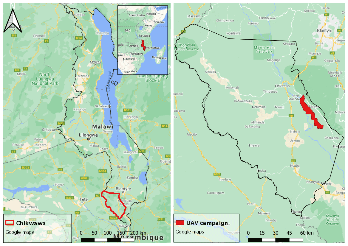
Figure 1The geographical location of Malawi (left) and the District of Chikwawa (right). © Google Maps, 2021.
In 2015, Malawi underwent some of the worst flooding ever recorded in the country, affecting 1 101 364 people, displacing 230 000, and killing 106. In the aftermath, it became clear that the housing sector accounted for most of the total damage with almost 40 % followed by agriculture with approximately 20 %. The worst affected districts were in the Southern Region, being the districts of Chikwawa and Nsanje, and the disaster sparked a discussion about a more responsible policy towards this type of event. One of the lessons learned from this event was that the lack of disaggregated (spatial) data and information management slowed down the disaster response and could eventually slow down recovery efforts as well (Government of Malawi, 2015).
Between 22 and 26 January 2019, the Chikwawa District was again subjected to extensive flooding because of continuous rainfall from Tropical Cyclone Desmond. There is no specific empirical damage data available for our case study area. However, the International Federation of Red Cross and Red Crescent Societies (IFRC) issued an Emergency Plan of Action (EPoA) after the floods. Based on preliminary assessment carried out by staff members and volunteers from the Village Civil Protection Committee (VCPC) and Malawi Red Cross Society (MRCS), one of the most affected areas is the Traditional Authority of Makhuwira with a total of 2434 collapsed houses (IFRC, 2019). In Chikwawa, a total of 15 974 people were affected, 3154 houses damaged or destroyed, and 5078 people reported to be displaced across at least seven camps set up by communities and government. Most of the affected houses were semi-permanent buildings, which are also common in our study area (IFRC, 2019).
In order to determine the hazard, exposure and vulnerability for both the pixel- and object-based approaches, a variety of data sources have been used. This section describes these data sources, including remote sensing and other geospatial data (including UAV imagery), local survey, regional building statistics, and the datasets used for the construction of (local) damage curves.
3.1 Remote sensing data
UAV imagery was collected in November 2018 by The Netherlands Red Cross (NLRC) and the MRCS for mapping and flood simulation purposes in the Lower Shire Basin. A fixed-wing UAV (SmartPlanes Freya) with 0.3 m2 wing area, weighing around 1.5 kg, and with a RICOH GR II camera was used to obtain the UAV imagery. The drone usually flew around 300 m altitude, having a flight time of around 60 min per battery and with a sidelap and overlap of each 70 %. The flights were carried out without ground control points (GCPs). Van den Homberg et al. (2020) give a detailed description of the UAV model and data collection. Agisoft PhotoScan and Metashape software was used to stitch the images of the optical imagery and extract a digital surface model (DSM) from the stereophotogrammetry. The extent of the flight coverage is shown in Fig. 1.
In addition to UAV imagery, other remote sensing data were acquired from open-source databases, including the Shuttle Radar Topography Mission (SRTM) digital elevation model (DEM) collected by NASA and the synthetic aperture radar (SAR) Sentinel-1 imagery collected by Copernicus (Farr and Kobrick, 2000). The High-Resolution Settlement Layer (HRSL) provides an estimate of the settlement extent and population density and was developed by the Connectivity Lab at Facebook in combination with the Centre for International Earth Science Information Network (CIESIN) by using computer vision techniques to qualify optical satellite data with a resolution of 0.5 m (CIESIN, 2016). The OpenStreetMap (OSM) contains a features layer of manually delineated objects and was used for validation purposes (© OpenStreetMap contributors, 2019). Table 1 summarizes the various datasets.
Table 1Available datasets in this research. Abbreviations: digital elevation model (DEM), digital surface model (DSM), ground range detected (GRD), Malawi Red Cross Society (MRCS), OpenStreetMap (OSM) and Shuttle Radar Topography Mission (SRTM) synthetic aperture radar (SAR).
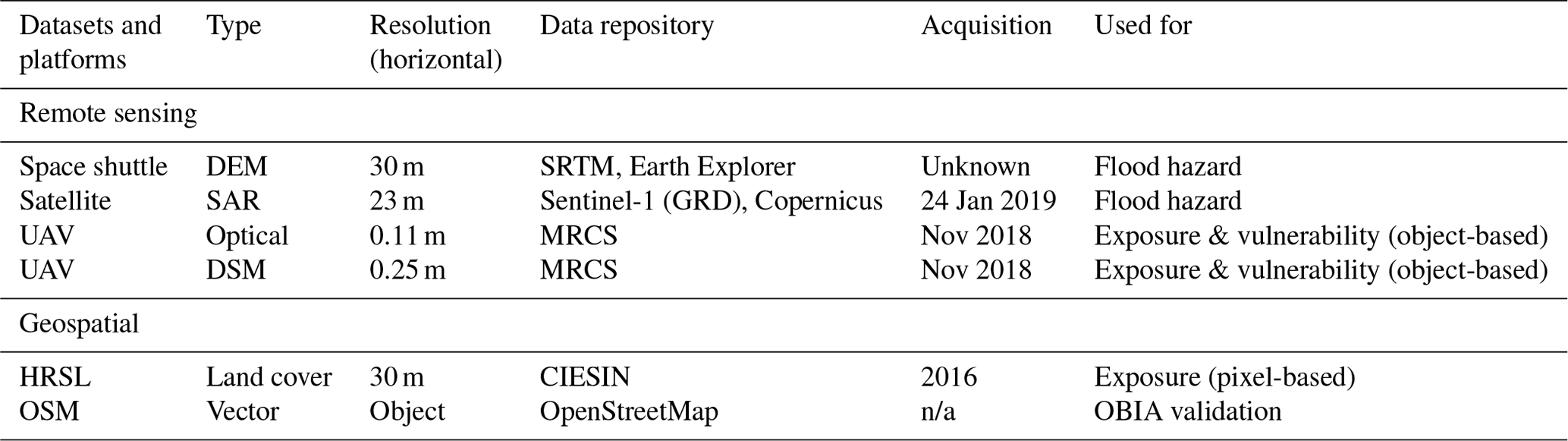
The term n/a stands for not applicable.
3.2 Building data
To gain information about the building stock present in the case study area, Teule et al. (2019) conducted a field survey in four villages in, or surrounding, the Traditional Authority Makhuwira (including Jana, Nyambala and Nyangu). The data were collected by randomly selecting buildings in the vicinity of these interviews. In total, 50 buildings were sampled and assumed to be representative buildings in estimating the different building characteristics present in the area. The OSM data layer reports on a total of around 1350 buildings in the villages selected for our analysis. Figure 2 shows an example of one the sample buildings. The survey collected characteristics of potential flood vulnerability parameters, including size, height, roof material, wall material and inventory of the house. These parameters were selected based on key features that characterize building types in the region along with their spectral differences, making them easier to detect from remote imagery.
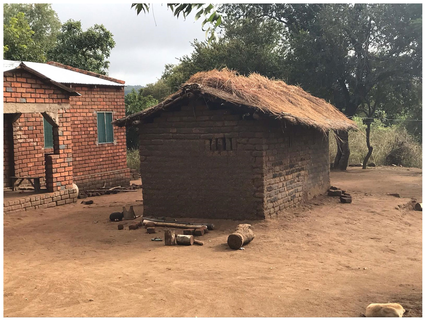
Figure 2Image from one of the sample buildings taken in the case study area taken by T. Teule (23 June 2019). A clear contrast between building material is visible between the two buildings: thatched roofs and unburned brick walls (middle building) versus iron sheeted roofs and burned brick walls (left building).
In addition to the local field survey data, building stock used in the pixel-based approach was extracted from the Integrated Household Survey 2016–2017 (IHS4), conducted by the Malawi National Statistical Office (NSO) (Malawi Statistical Office, 2017). This report describes the distribution of three main building types by aggregating data to a regional level. A distinction is made based on their building material:
-
A permanent building has a roof made of iron sheets, tiles, concrete or asbestos, and walls made of burned bricks, concrete or stones.
-
A semi-permanent building is a mix of permanent and traditional building materials and lacks the construction materials of a permanent building for walls or the roof. That is, it is built of non-permanent walls such as sun-dried bricks or non-permanent roofing materials such as thatch. Such a description would apply to a building made of red bricks and cement mortar but roofed with grass thatching.
-
A traditional building is made from traditional housing construction materials such as mud walls, grass/thatching for roofs and rough poles for roof beams.
Table 2Ratios of building stock in the Chikwawa District of southern Malawi (Malawi Statistical Office, 2017).
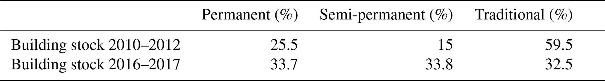
The ratio of the different dwellings in the district of Chikwawa is summarized in Table 2. From this information, a trend can be observed towards a ratio with more formal buildings. The most recent statistics – being the building stock information from 2016 to 2017 – is used in the pixel-based flood damage assessment.
3.3 Damage curve data
Stage-dependent damage curves are created for different building types by extracting material-specific vulnerability functions from the CAPRA (probabilistic risk assessment) platform. This platform contains a library with pre-defined analytical vulnerability functions, including different construction materials, calibrated with expert-supplied parameters (CAPRA, 2012). These curves express relative damage as a percentage with respect to water depth. Several examples in the library include concrete, wood, reed, masonry and earth (unfired) materials.
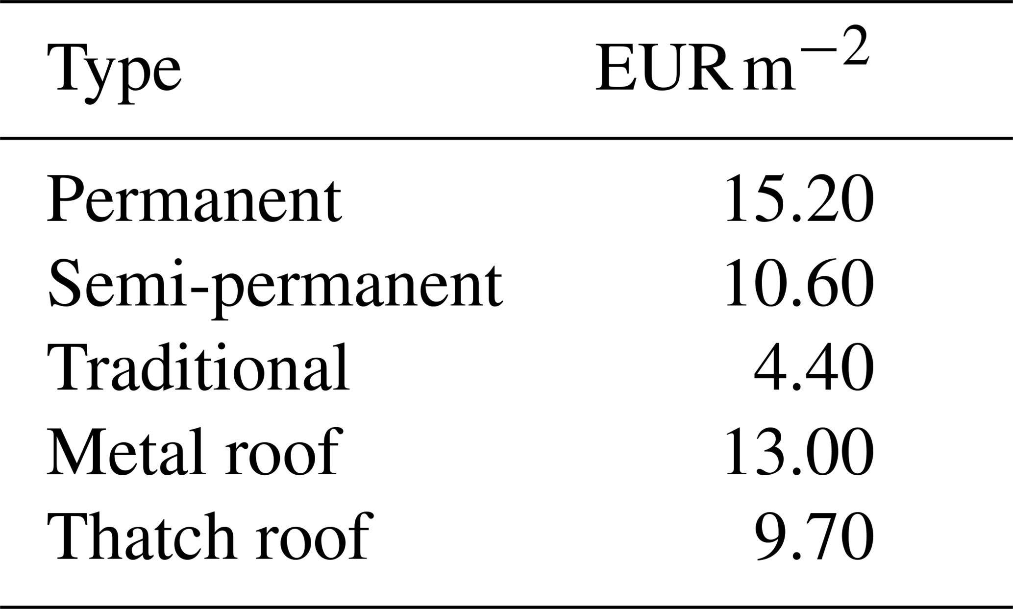
In addition to the vulnerability curves, maximum building damage values were estimated based on the different kinds of materials and the costs of buildings found in southern Malawi (Table 5). The values were validated by local authorities in the case study area during interviews by Teule et al. (2019).
This section describes the two flood damage assessment methods compared: first, the conventional pixel-based method and second the proposed object-based method, after which their distinctive components are discussed in more detail.
4.1 Flood damage assessment
Figure 3 presents the workflow applied in this study to derive the flood damage estimates from the January 2019 flood event in the case study area. Following the general procedure of a flood damage assessment, both approaches can be divided into three separate components: hazard, exposure and vulnerability (Merz et al., 2010; de Moel and Aerts, 2011; Jongman et al., 2012); see Fig. 3. In this research, we define the hazard as the flood extent and depth of a flood event, exposure as the exposed buildings to this flood, and vulnerability as the susceptibility of these buildings to flooding.
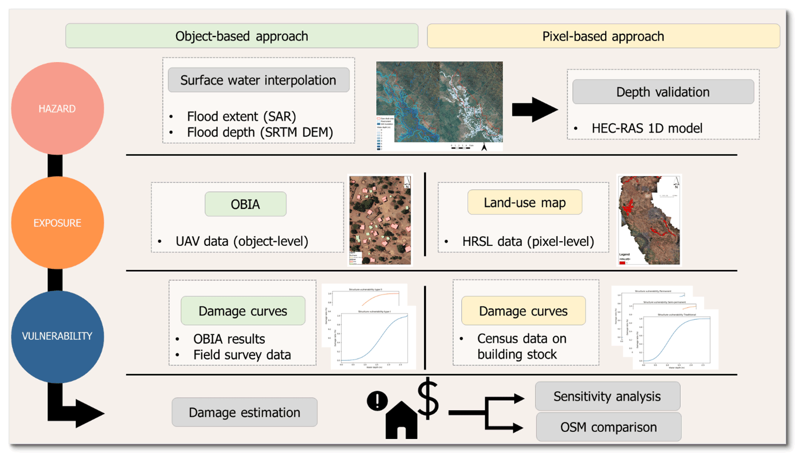
Figure 3Workflow of the two approaches of flood damage estimation. The left panel shows the object-based approach, and the right panel shows the pixel-based approach. Abbreviations: synthetic aperture radar (SAR), Shuttle Radar Topography Mission (SRTM) digital elevation model (DEM), object-based image analysis (OBIA), High-Resolution Settlement Layer (HRSL) and OpenStreetMap (OSM). The inundation (hazard) map is shown on a © Google Satellite image. The OBIA and land-use maps are created using UAV imagery from the Malawi Red Cross Society.
For the pixel-based approach, the HRSL land-use map, containing homogenous land-use pixels, is used to determine the built-up area. Building stock information from Table 2 is used to create corresponding stage-damage curves for the defined building types (Malawi Statistical Office, 2017).
For the object-based assessment, we combine information from an OBIA of high-resolution UAV imagery with the stage-damage curves created from the field observations. Building footprints are detected and classified based on their aerial features to identify local building types. Local stage-damage curves are then assigned to these types by assessing the vulnerability of buildings found in the field survey.
Both flood damage assessments are inherently different on the classification of exposed elements and their flood susceptibility. In the terminology of the UNDRR (2019), this translates into different input data for the exposure and vulnerability components.
The two different approaches share the same hazard component, being the 2019 flood event. Based on Sentinel-1 satellite imagery, a flood extent is created, and its related water depth is estimated. The economic damage is calculated by combining the flood impact with the different sets of exposure data and damage curves (Fig. 3). In order to determine the relative influence of the different components on the resulting risk, we evaluate the influence of building size, water depth and damage curve on our damage assessment model using a one-at-a-time sensitivity analysis, as applied in Ke et al. (2012).
4.2 Hazard: flood area and water depth estimation
To represent the flood hazard, we derive water depths from the January 2019 flood event using the workflow presented in Fig. 4. This approach takes the following three main steps: (1) extracting SAR data and processing them using SNAP software (SNAP, 2019) to create a flood extent map, (2) preparation of the data in ArcGIS, and (3) using the available SRTM DEM to estimate the water surface elevation and extracting the flood water depth.
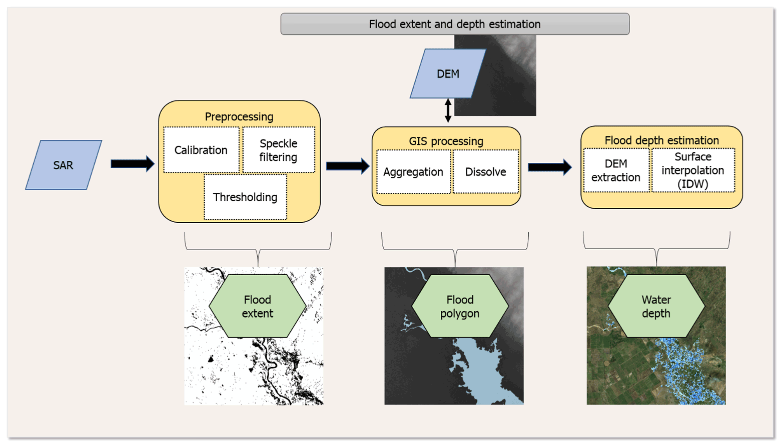
Figure 4The workflow representing the extraction of SAR satellite imagery and deriving its corresponding water depth. The flood polygon is shown on a SRTM DEM image, and the water depth map is shown on a © Google Satellite image.
Extracting and processing SAR data was based on the SNAP flood mapping workflow (McVittie, 2019). This involved preprocessing of the SAR imagery through calibration to transform the pixels from the digital values recorded by the satellite into backscatter coefficients, speckle filtering using the “Lee filter” to remove thermal noise and geometric correction using the terrain correction function. Water and non-water are separated through setting a threshold by analyzing the backscatter coefficient histogram and manually determining the peak characteristics of land and water areas. Flooded areas could then be determined by setting a threshold value of 0.0022 which was defined based on the histogram plot of pixel values for reflectivity.
The flood raster map was further prepared in ArcGIS by vectoring the resulting water pixels using the “raster to vector” tool and aggregating with the “aggregate polygons” tool based on a neighborhood of 100 m. Single-pixel polygons were removed to exclude noise from the flood map, and any empty spaces in the polygon were filled using the “union” and “dissolve” tools. These filled spaces can be the result of beneath-vegetation flood areas that can be missed by the SAR processing (Shen et al., 2019). Negative values are removed in the next, final step if they are a result of actual topographic factors, such as local hills.
The final step in this approach follows the research of Cian et al. (2018) and Cohen et al. (2018), in which the flood boundaries along the water surface are used to estimate the elevation of the water surface. The boundaries of the derived flood extent were turned into points with the “raster to point” tool, after which the elevation values were extracted from the DEM. The water surface was then computed using the “inverse distance weighting” (IDW) tool. Essentially, this means that pixels inside of the flood extent get the elevation value of the closest elevation points along the boundary. The water depth can then be calculated by deducting the initial DEM values from the assigned water surface values. Figure 4 visualizes the workflow and the resulting output.
To validate the surface water interpolation method, the result is compared with a flood hazard map obtained from a hydraulic 1D steady model that was run for a subsection of the Shire River (Maparera River) in a study by Copier et al. (2019). The segment covers an area of 2.1 km2 in which the river has a total length of 2.2 km. The model was run using Hydrologic Engineering Center's River Analysis System (HEC-RAS) software (Hydrologic Engineering Center, 1998). Due to a lack of historical data, the discharge values used as input for the model are estimated to match the case study area's water flowing abilities without creating an extreme overflow. The discharge value was set to 50 m3 s−1, and the Manning coefficient was set to 0.05. For both the surface water interpolation method and the hydraulic model run, the UAV DSM is used as input.
The root mean square error (RMSE) is used to evaluate the output from both approaches (Cohen et al., 2018). By doing so, it can be determined to what extent the output of both approaches deviate in terms of water depth estimation. In addition to the root mean, we also construct the receiver operating characteristic (ROC) curve. The ROC curve is a probability curve and reports the true positivity rate (TPR), also called recall (R), as a function of the false positive rate (FPR). The area under curve (AUC) represents the degree or measure of separability, with 1 representing a model with a perfect predictability, 0 with complete unpredictability and 0.5 with random guesses. The HEC-RAS flood map is taken as ground truth against the results of the surface water interpolation method, in which a prediction can be either a true positive (TP), false positive (FP), true negative (TN) or false negative (FN). The TPR and the FPR are calculated as follows:
4.3 Exposure
4.3.1 Pixel-based approach
For the pixel-based approach, the built-up area is estimated by taking the built-up area of the pixel according to average density percentages and building sizes. This density is determined by visual interpretation of the UAV imagery. The percentages found in the distribution of building types reported by the IHS4 are used to calculate the damage corresponding to 1 pixel unit.
4.3.2 Object-based approach
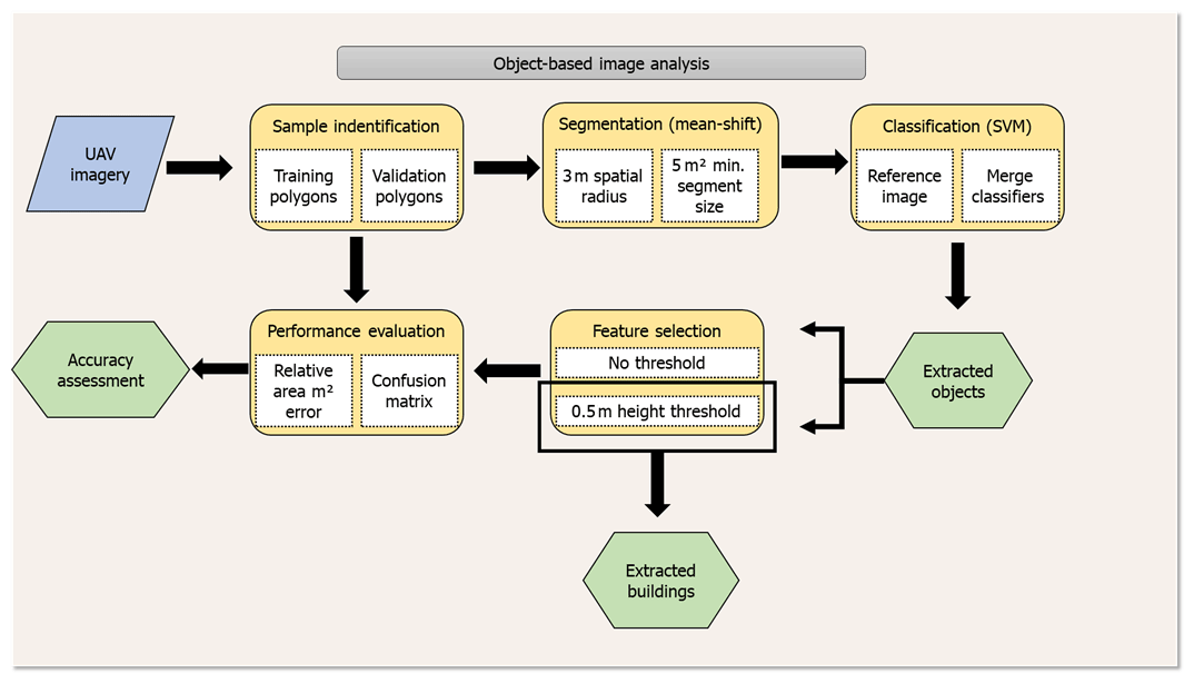
The OBIA consisted of the following steps (Fig. 6). First, validation and training samples were collected from the villages in the case study area by manually delineating objects. We manually delineated a total of 144 building to serve as training and 556 as validation. This step was followed by segmenting the high-resolution imagery and classifying the vectorized objects. We selected the open-source geo-software Orfeo ToolBox (OTB). This toolbox is a library for image processing initiated by the CNES (French Space Agency) that includes numerous algorithms created for the purpose of segmentation and classification (Grizonnet et al., 2017).
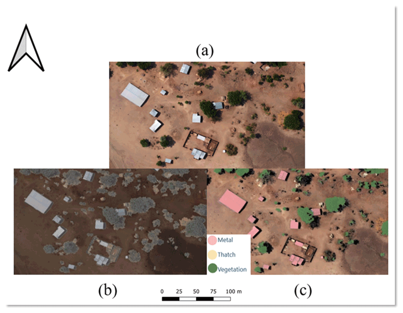
Figure 5Steps of the OBIA: (a) original UAV imagery, (b) result of mean shift segmentation and (c) classification using SVM classifier. The image contains UAV imagery collected by the Malawi Red Cross Society (MRCS), collected in November 2018. Made with QGIS.
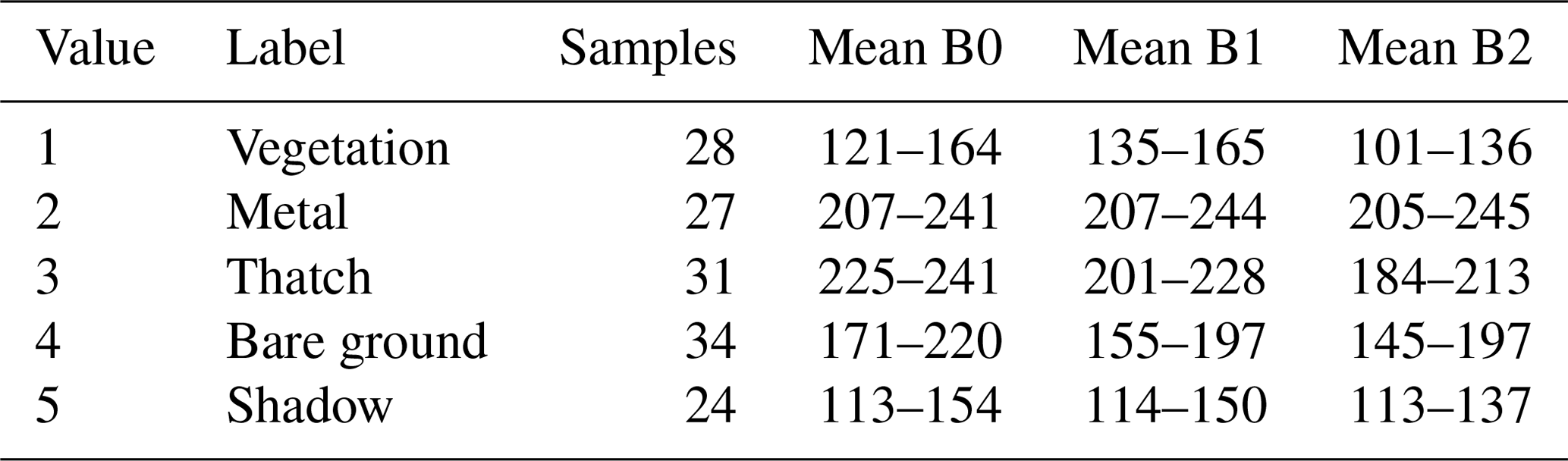
Segmentation was performed using the mean shift clustering algorithm utilized by OTB. The mean shift algorithm exploited by Orfeo relates to the work of Michel et al. (2015), in which the goal of image segmentation is to partition large images into semantically meaningful regions. The following parameters were set: (1) the spatial radius or the neighborhood distance was set to 1.5 m, (2) the range is expressed in radiometry units in the multispectral space to 5 m, and (3) the minimum size of a segmented region was set to 5 m2 in relation to minimum building sizes. The support vector machine (SVM) algorithm from the same Orfeo library served to classify the vectorized objects from the segmentation. The SVM is a kernel-based machine learning algorithm that has been effectively used to classify remotely sensed data (Mountrakis et al., 2011). The classifier was trained on samples that represented the common features in the selected images and are summarized in Table 3. An example of the output of this process is shown in Fig. 5.
Table 3Samples used as input for training the SVM classifier with mean value ranges of the spectral bands (nm).
After the segmented objects were classified, a filtering process was conducted in which objects were removed based on their respective height and category. By keeping the two categories that represent buildings with a height over 0.5 m, buildings can be extracted, and potential misses are excluded from the damage calculation. This height was chosen as a value between the height of the ground and a one-story building. The mean height from the DSM was added to the objects by creating centric points of each segment and extracting the elevation values to these points from the UAV DSM map. To derive the height of these objects, a baseline DEM was constructed and subtracted from the mean DSM value. For this, the cells classified as “metal” and “thatch” were removed from the DEM. Next, ground reference points were placed using visual interpretation to make sure no bushes or trees were selected. The elevation of these ground reference points was correspondingly used to interpolate an elevation surface using IDW, and the elevation of this interpolated surface was used to determine the height of the metal and thatch cells by determining the difference with the original DEM elevation.
To evaluate the performance of the OBIA model, a map with 556 manually delineated and labeled reference buildings was compared to a map with predicted buildings from the classification. For this purpose, a confusion matrix was created (Gutierrez et al., 2020), in which TP is the number of cases detected both manually and with the automatic approach. FP is the number of cases detected by the automatic approach but not manually. TN is the number of cases detected manually but not by the automatic approach. FN is the number of undetected cases. The statistical parameters that were used to test the classification performance are the accuracy and F1-score. The overall accuracy (A) was calculated given Eq. (1).
To test the classification performance per class, the F1-score was used. This statistic is the weighted mean of both precision (P) and R, where 0 indicated the lowest possible score and 1 a perfect score. The parameters are calculated with the following equations:
To evaluate the building area, predicted buildings were chosen that have partial or complete overlap with the reference buildings. From this selection, the relative error (RE) was calculated per building type. In this case, the absolute error is normalized by dividing it by the magnitude of the value of the reference buildings. The RE is calculated through the following expression:
where θ∧ is the predicted value, θi is the value of the reference buildings, and N is the sample size.
4.4 Vulnerability: damage curve estimation
Corresponding to the building types found in the exposure component of each flood damage assessment, a set of damage curves is created. The description of the different types and their construction material is used to weigh material-specific damage curves from the CAPRA library, according to the method proposed by Rudari et al. (2016). We make use of the expanded aggregation table as proposed by Rudari et al. (2016), including the construction material considered for every building type (Table 4). This table indicates for each building type the building stock material for which CAPRA damage curves are used.
Table 4Aggregation table of the CAPRA damage curves based on building stock information.

For the pixel-based approach, three curves are created for each of the building types (traditional, semi-permanent, permanent), making use of the description of wall building materials in the fourth Integrated Household Survey 2016–2017 (IHS4). Next, the distribution of these three building types (Table 2) is used as weights to create a single curve that can be applied to the urban pixels from the land-use map. For instance, semi-permanent housing consists of unburned bricks, for which the masonry and earth CAPRA curves should be used. In this case, these curves are averaged and used to represent a semi-permanent building.
For the object-based approach, the results from the field survey are used to create damage curves for building types determined by aerial observation and the OBIA (metal roof and thatch roof). The materials of the roofs are correlated with wall material, based on the field observations from which we derive the wall-to-roof relationships. The local distribution found in wall material is used to weigh the curves from the CAPRA library based on percentages. This means, for example, that the distribution in wall material found for buildings with a thatch roof – being burned bricks, unburned bricks, mud and wood – are used to weigh the CAPRA curves. These materials correspond to the masonry, masonry and earth, and earth and wood CAPRA curves, respectively.
In both approaches, we follow Maiti (2007) and assume that buildings constructed with a mud wall tend to collapse at a water depth of 1 m. Before creating curves for each building type, this damage curve from the CAPRA library (earth curve) is modified so that 1 m of inundation corresponds to a 100 % damage value.
4.5 Risk: damage estimation
For the pixel-based approach, the built-up area is estimated by taking the built-up area of the pixel according to average density percentages and building sizes. The average density percentages and building sizes will be collected by visual interpretation of the UAV imagery. The percentages found in the distribution of building types reported by the IHS4 are used to calculate the damage corresponding to 1 pixel unit. The damage is calculated through the following expression:
where the variables are as follows:
-
ip is the building type (i.e. traditional, semi-permanent, permanent) as determined by the building stock description of the Malawi National Statistical Office (2017).
-
damage(ip) is the damage per pixel in euros calculated with the adjusted stage-damage curve and using as input the water depth (m) in the considered pixel.
-
a(ip) is the size of the building in area (m2).
-
r(i) is the ratio of the type according to the national survey in Table 2.
-
rc(i) is the replacement cost per square meter based on the type (i); see Table 5.
For the object-based approach, damage is calculated per object by combining buildings automatically detected and classified through OBIA with the local stage-damage curves created from the field survey. The damage can be calculated through the following expression:
where the variables are as follows:
-
io is the building type based on the roof type and wall-to-roof relationships (i.e. metal roof and thatch roof).
-
damage(io) is the damage per building in euros calculated with the local stage-damage curve and using as input the flood water depth (m) for this building.
Table 5Estimated maximum damage values per square meter based on local knowledge of replacement costs (Teule et al., 2019).
4.6 Sensitivity analysis
To quantify how the damage parameters can influence the damage estimate, a one-at-a-time sensitivity analysis will be conducted by increasing and decreasing the different damage parameters with the mean of the respective relative errors. The sensitivity value (SV) will be used to represent the sensitivity and can be calculated by dividing the largest resulting damage by the smallest resulting damage (Koks et al., 2015).
5.1 UAV imagery
Figure 7 shows the resulting UAV-based orthophoto, including the DSM with shaded relief and the SRTM DEM with shaded relief, from the flight area. The Shire River is captured at the western side of the acquired imagery. Completing the area took 140 flights, each lasting around 45 min. The UAV-based DSM shows a relatively equal elevation throughout most of the area. However, the absence of GCPs influenced the global accuracy of the elevation. A deviation can be observed when we compare the UAV-based DSM to the SRTM DEM. This DEM shows a down-sloping pattern of the elevation towards the south, in accordance with the flow of the Shire River.
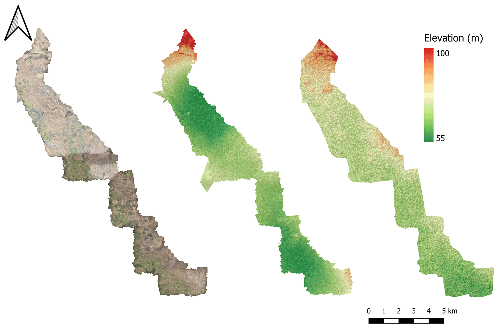
Figure 7Example of the orthophoto (left) and DSM (middle) with shaded relief, produced with images from the UAV flight, and a Shuttle Radar Topography Mission DEM (right) with shaded relief. Made in QGIS using UAV imagery collected by the Malawi Red Cross Society (MRCS).
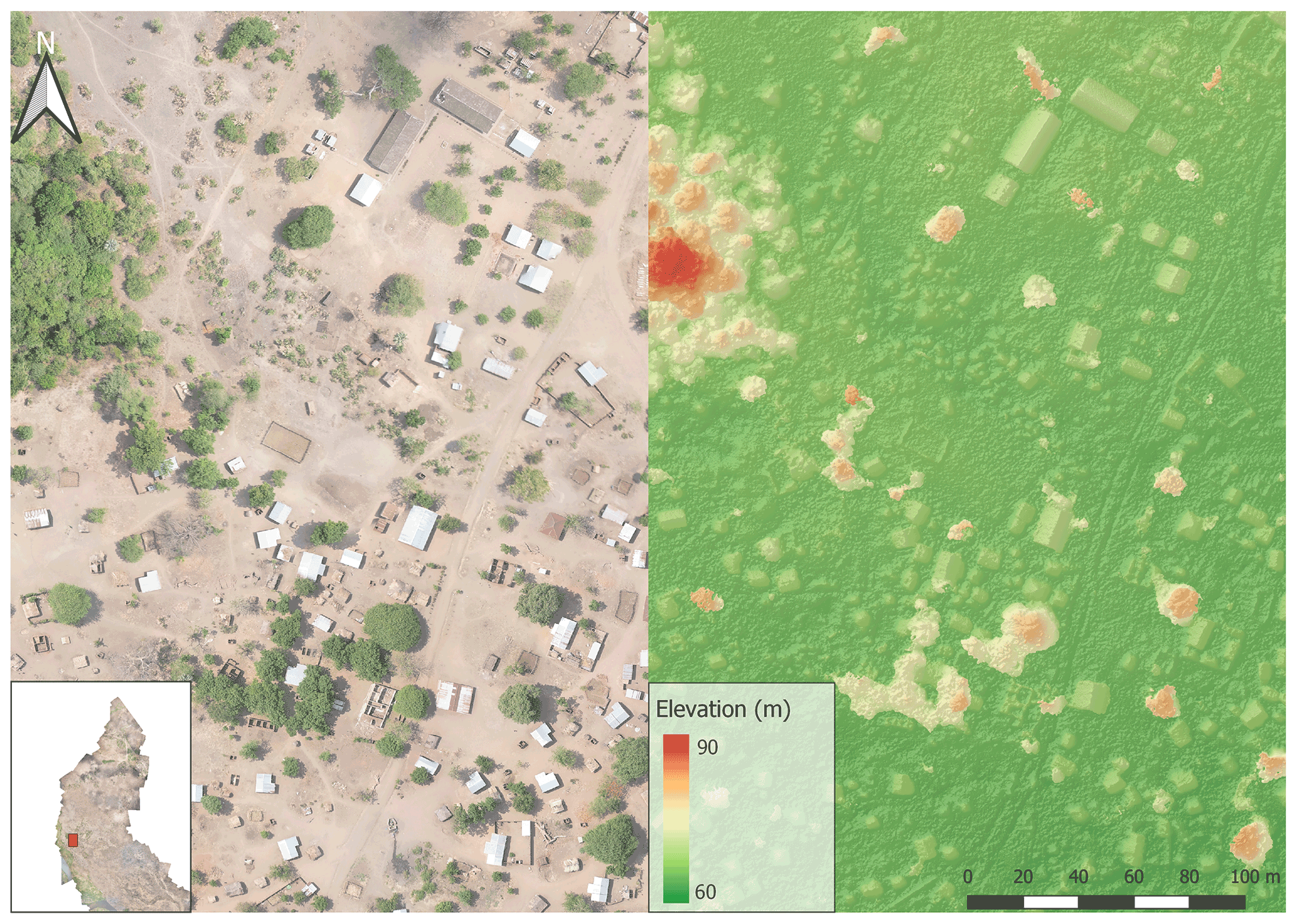
Figure 8Section of the town of Chagambatuka in the northern part of the UAV campaign area, with orthophoto (left) and DSM with shaded relief (right) produced with images from the UAV flight. Made in QGIS using UAV imagery collected by the Malawi Red Cross Society (MRCS).
Although this difference hampers large-scale (hydraulic) analysis using the UAV-based DSM, it is still valuable in assessing the local height variation of objects on a microscale. Figure 8 gives a detailed overview of the town of Chagambatuka, including the UAV-based DSM. Buildings can clearly be distinguished based on their rectangular shape and elevation, while trees are generally the tallest objects in the area.
5.2 Field observations
Based on the information collected through the building survey, buildings in the case study area are grouped into two types based on their distinctive aerial features. From the 50 samples, no buildings were found that have a wall structuring resembling wood, reed or concrete. In addition, no buildings were found having tiles or any other material as the roof, nor any having more than two levels.
The first type of building in the area is composed of burned and, in a small number of cases, unburned bricks. This type is less vulnerable to flooding compared to the other type due to its material being less susceptibility to building failure. Its main distinctive aerial feature is a metal sheet roof, but the results of the OBIA and the field survey also indicate that this type of building has a larger footprint than thatch-roofed buildings. For the metal-roofed buildings, two wall materials were found: burned red bricks (90 %) and unburned bricks (10 %).
The second type is generally composed of less formal building material, with its main distinctive feature being a thatch roof. The results of the survey seem to indicate a relatively equal distribution between the building materials, but as unburned bricks and mud walls are more susceptible to building failure, this type is considered more vulnerable to flooding. For the thatch-roofed buildings, three wall materials were found: burned red bricks (27 %), unburned bricks (41 %) and mud/wattle (32 %).
5.3 Damage curves and maximum damage values
Figure 9 shows the two damage curves created for the object-based approach based on types corresponding to the field survey (left) and three for the types in the building stock description of IHS4 national survey that are used in the pixel-based approach (right). Metal-roofed buildings show a lower vulnerability than thatch-roofed at the same water depth due to the structural integrity accompanied by more formal building material. Similar patterns can be observed for the damage curves based on the description of building stock in the Chikwawa District. Similar to how the damage curves were derived, maximum damage values have also been determined. The damage values per square meter for all building types can be found in Table 5.
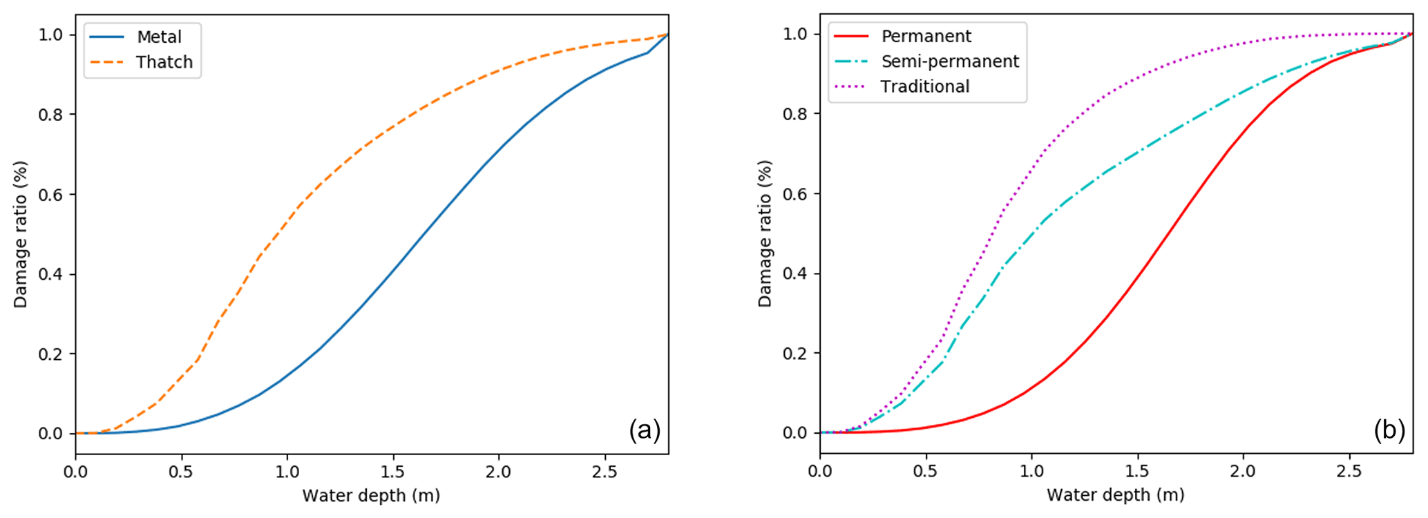
Figure 9Constructed damage curves for the two types derived from field and aerial observations for the object-based approach (a), and three types derived from the description of building stock at district level for the pixel-based approach (b) (Malawi National Statistical Office, 2017). The water depth is the flood water relative to the ground floor.
5.4 OBIA quality assessment
The implementation of the OBIA model had a varying degree of success according to the statistical tests. Table 6 shows that classification is more reliable for classifiers that have a clear spectral difference with surrounding elements, such as shadow and metal roofs, whereas bare ground and thatched roofs are less easy to distinguish. This spectral difference resulted in a higher F1-score for buildings with a metal roof (89 %) compared to those with a thatched roof (53 %). With the F1-score being the harmonic mean of the precision and recall, this metric captures both the false negatives and the false positives of the classification process. The lower F1-score for detected thatch roofs could be attributed to their tendency to blend in with the environment because of their relatively similar spectral properties. With the addition of the height threshold for objects, the individual F1-scores for buildings were improved to 90 % for metal-roofed buildings and 72 % for thatch-roofed buildings. The increased F1-score for thatch-roofed buildings indicates that having additional and accurate information on the height of the objects has a large effect on the individual classification accuracy. The overall accuracy of the initial run shows a value of 77.45 %, indicating the amount of correctly classified objects out of the total amount of samples. This value also increases up to 80 % with the addition of a height threshold for objects, though this increase is also partly due to the exclusion of poorly performing classes such as “bare ground”.
Table 6Evaluation of the performance accuracy of the OBIA classification.

* Addition of height threshold by subtracting the extracted DSM and DEM values.
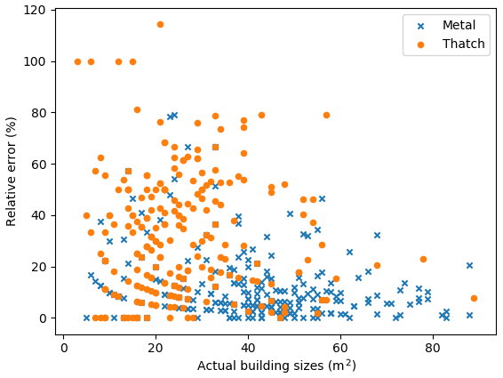
Figure 10Building area and relative error for both types (metal and thatch) in the case study area.
The building objects from the OBIA are a direct result of the segmentation process, and the relative error seems to reflect the same pattern as the classification process. This means that buildings with a thatch roof tend to be harder to detect because the model groups pixels together that represent different objects, such as bare ground and the thatch roof. For both types, the relative error between observed and predicted building areas can be observed in Fig. 10. For the thatch-roofed buildings, 50 % of the predictions are found with RE lower than 30 %. For the metal-roofed buildings, this same percentage of predictions are found with a RE lower than 7.5 %. Generally, metal-roofed buildings tend to be larger in size than thatch-roofed buildings, with a mean building size of 39 and 21 m2, respectively. For both types, the RE tends to decrease as building size increases. This seems to be in line with the literature in which it is stated that if objects get closer to the size of the available spatial resolution, errors are more likely to occur (Blaschke, 2010).
5.5 Flood inundation
To check whether the surface interpolation method adequately captures flood characteristics, we compare our method with the results from a hydrodynamic model applied at the Maparera River. Figure 11 shows the maximum water depth obtained from both methods. The average water depth from the flood event at the Maparera River was 1.17 m for the surface water interpolation and 1.22 m for the hydraulic model run using the UAV DSM (Copier et al., 2019). The maximum estimated water depth for both approaches was about 3 m (3.30 and 2.79 m, respectively). The RMSE was calculated to be 0.73 m. The results show that for a flood depth of approximately 3 m, the surface water interpolation method deviated from the hydraulic model by <0.75 m on average. We found considerable differences between both models along the main channel. This is in line with research from Cohen et al. (2018) given the inability of similar methods to calculate complex fluid dynamic effects. In addition, the interpolation method shows relatively low water depth at the upstream boundary compared to the hydraulic model. Nevertheless, the interpolation model seems to correctly dissolve the higher-elevation area between the two main channels from the aggregated flood extent that was extracted from Sentinel-1 imagery. The AUC measured 0.73 (see Fig. A1), indicating an acceptable agreement between the HEC-RAS reference map and the water depth map resulting from surface water interpolation (Hosmer and Lemeshow, 2000).
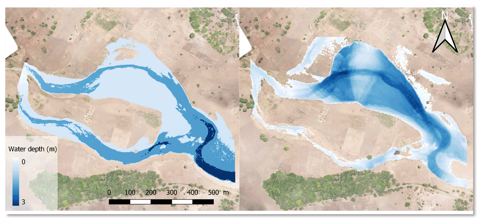
Figure 11The estimated water depth from the HEC-RAS hydraulic model (left) and the derived water depth following the surface interpolation method (right) at the Maparera River. Made in QGIS using UAV imagery collected by the Malawi Red Cross Society (MRCS).
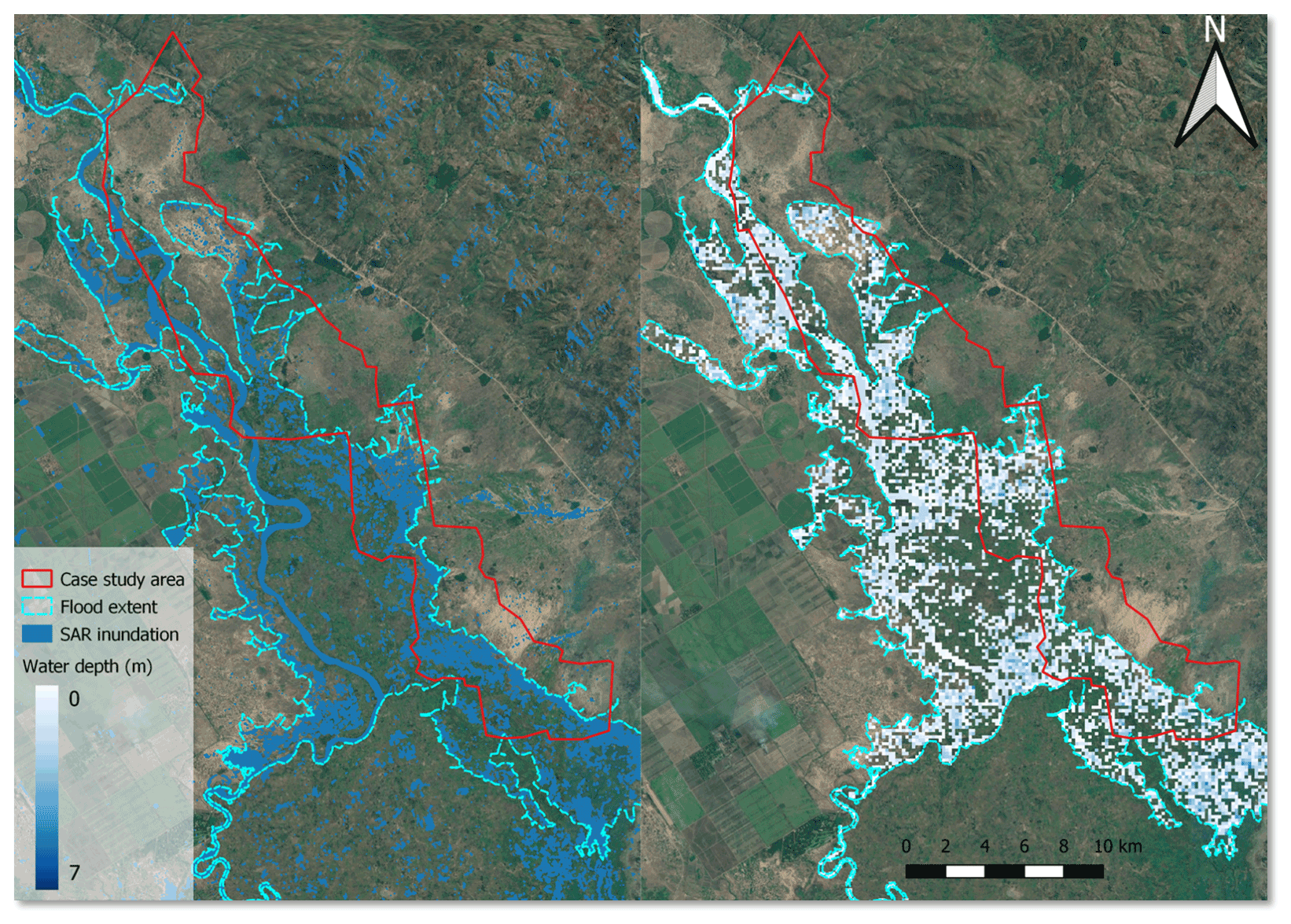
Figure 12The flood extent for the case study area extracted from SAR imagery (left) and the derived water depth map using surface water interpolation based on the SRTM DEM (right). The inundation maps are shown on © Google Satellite images.
Repeating the method for the total case study area with the SRTM DEM produced a water depth map with an average water depth of 1.26 m and a maximum water depth of 7 m (see Fig. 12). Buildings in the inundated area were assigned the water depth in the corresponding cell. Several areas with a positive water depth can be observed in the resulting flood map that deviate from the SAR inundation map. These areas indicate the subtraction of incorrect water depth values from the digital terrain model (DTM) or capture areas that were not identified with SAR imagery, for example, due to high vegetation.
5.6 Damage estimates
By overlaying the separate components of the flood damage assessment, the estimated damage was calculated for both approaches using Eqs. (7) and 8. Compared to the pixel-based approach, the object-based approach provides a lower estimation of the exposed built-up area of about two-thirds (Table 6). Interestingly, comparing the number of buildings in OSM, this comes very close to the amount extracted by the OBIA, giving confidence in the object-based approach. This amount of exposure influences the resulting damage considerably. The flooded built-up area for the pixel-based approach and the object-based approach was estimated at 2541 and 3952 m2, respectively. This resulted in estimated flood damage of approximately EUR 10 000 and EUR 16 000, respectively (Table 6).
Table 7Flooded buildings and built-up area according to (1) the object-based approach, (2) pixel-based approach and (3) the available OSM map, as well as area and total damage according to (1) the object-based approach and (2) pixel-based approach.
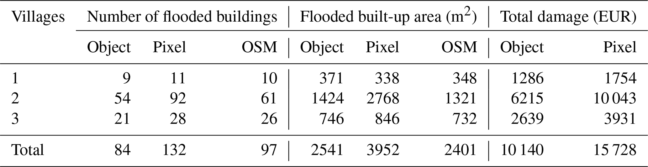
Although building densities and average buildings sizes were extracted from the same UAV imagery, a difference can be observed in the flooded built-up area between the two approaches. This is the result of the inability of land-use pixels to account for spatial variability in the building objects inside a certain area.
Similar research on flood events in urban and rural areas in Ethiopia, Germany and Poland exemplifies that significant uncertainties are present in flood damage assessments due to information lacking on the number of flooded buildings, the building types considered in the assessment and the distribution of building use within the flooded area (Merz et al., 2004; Englhardt et al., 2019; Nowak Da Costa et al., 2021).
5.7 Sensitivity analysis
By varying the building size and water depth parameters with the mean of the respective relative errors, the sensitivity of the damage parameters for both approaches was estimated. As there is no information on the uncertainty of the damage curve values from the CAPRA database, the influence of this parameter is derived by using only the lowest and highest damage curves from the building types. For example, the lower damage bound for the damage curve sensitivity value in the object-based approach is computed by using only the metal-roofed damage curve and the higher bound using the thatch-roofed damage curve. Table 7 shows that the largest variance in resulting damage is caused by this variance in the damage curves, meaning that the damage curve selection has the highest effect on the resulting damage estimates.
Table 8The sensitivity values (SVs) of the different damage parameters for the pixel- and object-based approaches.
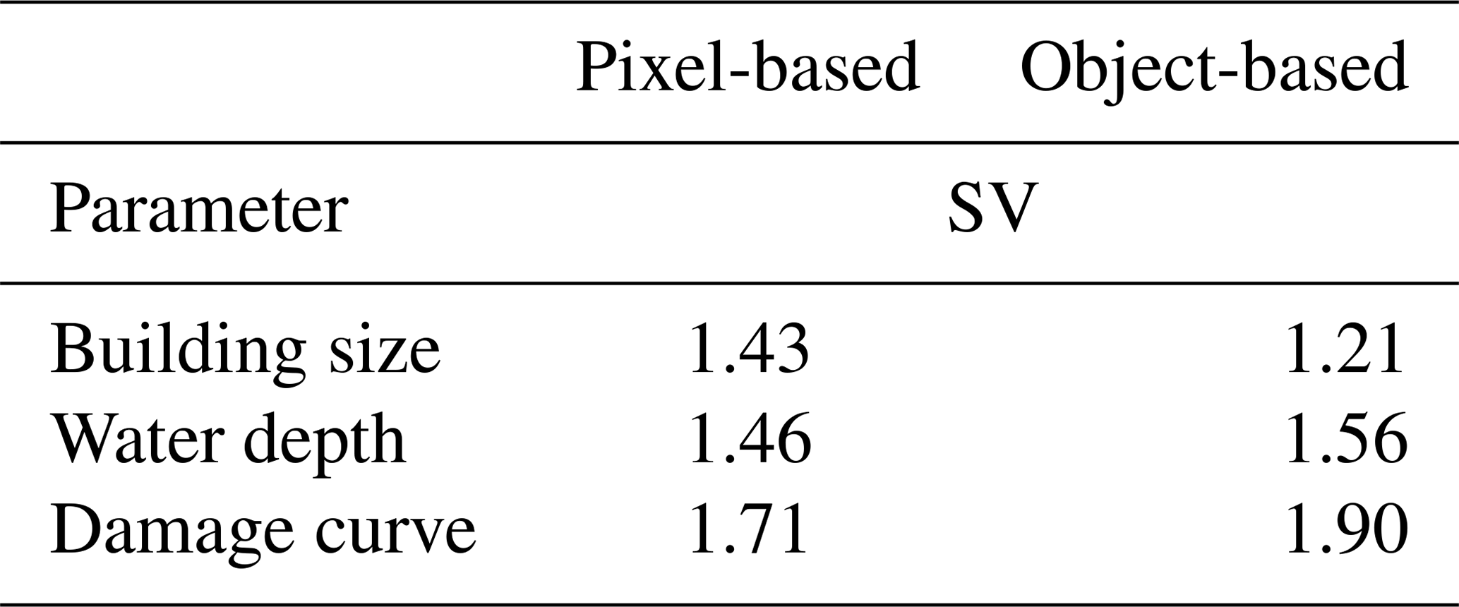
Similar results have been found by Saint-Geours et al. (2015) in a cost-benefit analysis of a flood mitigation project in which the uncertainty in the depth–damage curves is the prominent factor for estimating damage to private housing. Studies by de Moel et al. (2012) and Winter et al. (2019) also note that the most influential parameter in the uncertainty of flood damage estimates is the damage function. Moreover, it can be observed that the sensitivity value of building size is lower in the object-based approach compared to the pixel-based approach (1.21–1.43), which can be attributed to less uncertainty in total building area that is flooded. This indicates that, for the object-based approach, the increased accuracy with which buildings can be identified leads to a decrease in the uncertainty of damage estimates. The water depth parameter reveals that, although uncertainty in water depth results in varying damage estimates, sensitivity values for both approaches are comparable (1.46–1.56). Therefore, considering the same flood impact in each flood damage assessment does not affect damage estimates differently.
It is apparent from Table 7 that all parameters involved in the flood damage estimation include an amount of uncertainty, and this propagates in the total estimated damage. As the flood map in both calculations remained equal, the differences can be attributed to the sensitivity of the damage parameters to the building types and damage curve parameters or the exposure and vulnerability components.
The preceding sections illustrate that by using OBIA, flood damage can be estimated at the object level using UAV-derived imagery to detect buildings and classify them based on aerial features. This contributes to the literature in several ways. Complementing a study by Englhardt et al. (2019), which provides an impressive first glance at studies that use object-based data to classify buildings into vulnerability classes, our approach enables us to use this information to calculate damage at the individual building level. Therefore, our method provides more certainty on the number of flooded buildings, their size and location. A more recent study by Malgwi et al. (2021) suggests that using data-driven approaches, such as multivariate damage models, could further improve estimates in data-scare regions compared to more expert-based approaches. However, this is not always feasible if the scarcity of empirical loss data hinders the implementation of multivariate models, as is the case in most developing countries. Our study indicates, however, that OBIA combined with local data can accurately estimate flood damage in an area where such data are absent, for example, due to its remoteness.
Although this research has uncovered several important factors in the estimation of flood damage based on building detection, the issue deserves further additional research. First, the method was created for a specific case study area with little variation in building types. Building extraction is herein limited to the available building stock in the area, in this case resulting in two types. For urban areas, classification confusion might occur due to the heterogeneity of building types and structural properties. This complication could yield more uncertainties in assigning appropriate damage curves to buildings, especially as large discrepancies in potential flood damage exist between urban and rural areas in developing countries (Englhardt et al., 2019). Another distinction should be made between when studying areas with river floods or flash floods, as capturing the latter with earth observation data becomes a challenging task due to the low frequency of satellite imagery acquisition (e.g. SAR acquisitions) relative to the sudden happening of flash floods (Mouratidis and Sarti, 2013).
Secondly, the filtering of objects using the DTM deserves further attention. Evidently, the addition of an object height threshold by using the DTM does indeed lead to a significant improvement in accuracy of the OBIA. In our study, the baseline DEM was constructed by manually setting reference points. The method was successful as brushes and trees that resembled bare ground could be avoided, and the absence of ground control points during the UAV mission did not hamper the analysis. However, this method does rely on manual filtering, a process that is hard to scale and prone to human error. Preferably, this method should be automatized. Several novel methods to extract bare earth surface can be considered in the future, including open-source filtering methodologies such as the cloth simulation filter plugin developed by CloudCompare. Zeybek and Şanlıoğlu (2019) discuss several filtering algorithms that can reach excellent accuracies using high-resolution point cloud data collected by UAV. Considering this approach in future research could enhance accuracy while simultaneously improving reproducibility and scalability. Along with additional automatization, altering the OBIA workflow by including the height threshold before image segmentation could potentially improve classification results. Kamps et al. (2017) report that the classification accuracy of their OBIA improved by 15 %–26 % following this workflow but note that combining orthophotos with elevation data could potentially lead to the propagation of errors due to mismatches in datasets.
The third aspect refers to the additional field survey. The acquired building samples and their wall-to-roof ratios provide insight into the relations between the local elements and the remotely sensed characteristics. However, a larger number of samples would be necessary to provide a statistically sound justification of the assumption about this relation. Obtaining field observations could become a difficult task if the method is scaled up, but a promising line of research could be the implementation of services like Mapillary or Google Street View for this purpose. Combining the findings from this kind of research with field surveys can, therefore, complement the conventional methods by aggregating accurate estimates on building sizes, density and characteristics. This would decrease the amount of uncertainty incorporated in potential scaled-up assessments. The HRSL provides an impressive first glance at exposed settlements and can be used as a base layer to project the distributions of building exposure and vulnerability found in this study. This method resembles the study of De Angeli et al. (2016), in which clusters are created using representative buildings. In this case, field observations from drones and services like Mapillary can be combined to create representative villages or towns.
Finally, the other sources of uncertainty accompanied by the damage estimation need to be further studied. Although they do not directly relate to the results of the exposure estimation, the sensitivity analysis in this research confirms that parameters such as floodwater characteristics, maximum damage values and the applied damage curves have a significant effect on the total flood damage. The RMSE of about 75 cm and AUC of 0.73 illustrate that deriving water depths directly from a DEM can give results different from the hydraulic simulations. It should be noted that both methods have their disadvantages. In the hydraulic simulation, for instance, Copier et al. (2019) lacked specific discharge information for the event, so an estimate had to be made there that would resemble flood levels. The surface water interpolation method, on the other hand, lacks the dynamics of the hydraulic simulation but is more specific to the event considered in this study as it is based on the observed extent. To validate the water depth estimation, the effects of using a coarser-resolution SRTM DEM in surface water interpolation should be tested. Preferably, validation data from hydraulic models are used that correspond to the flood event that is extracted from satellite imagery. In this way, differences due to discharge uncertainties are limited. Another way of validating flood events is through the collection of community-based data. By interviewing residents, ground-based observations can be collected in ungauged areas to serve as input for detailed catchment modeling and validating output (Starkey et al., 2017). Also, the aggregation of damage curves based on building material could yield uncertainties in the resulting flood vulnerability. For a more accurate appropriation of the damage susceptibility, individual building types could be subjected to detailed survey studies that include historic flood events and damage with the corresponding building material.
The purpose of this research was to create a flood damage model based on the automated recognition of buildings and their characteristics through UAV image processing. By doing so, improvements on the exposure and vulnerability component of flood damage assessments were assessed and evaluated by comparing this new approach to a conventional one based on pixel-based information from a land-use raster. The two flood damage models were applied in a rural and flood-prone area in southern Malawi, with a building stock consisting of mostly semi-permanent buildings.
In terms of direct damage considering the replacement costs of buildings in the study area, the flood damage based on homogenous land-use pixels is about 50 % higher than the object-based approach (EUR 15 000 versus EUR 10 000, respectively). The calculation is found to be most sensitive to the damage curve used, with a sensitivity value (highest divided by lowest estimate) of 1.71 and 1.90, for the pixel-based and object-based approaches, respectively. However, uncertainty in building exposure still results in sensitivities of 1.43 for a pixel-based approach and 1.21 for an object-based approach. This illustrates that accurate information on exposure is essential in accurately estimating potential damage from flood events.
The effects of including high-resolution elevation information in the OBIA were examined by including a height threshold for classified objects. Individual F1-scores of the object-based classification were improved from 0.89 to 0.90 for metal-roofed buildings and 0.53 to 0.72 for thatch-roofed buildings. These results show that the integration of accurate elevation data can improve standard classification schemes based solely on spectral bands. The relative error of the area of the detected buildings tends to be lower for larger buildings and buildings with a clear spectral difference from the surrounding area. The water depth, derived by interpolating the surface water boundaries of a remotely sensed flood extent, deviated on average by 0.73 m from a hydraulic model for a maximum water depth of approximately 3 m. This validation was conducted for a subset of the case study river using a high-resolution DSM. For the same area, the obtained AUC is 0.73.
Based on the results of this study we find that the primary utility of high-resolution UAV imagery in flood damage assessment is to spatially locate buildings in inundated areas and retrieve their characteristics by creating types in combination with local observations. These characteristics can be used to develop stage-damage curves that represent the local building stock instead of using aggregated information that implies homogeneous land cover for large regions. Furthermore, the number of buildings and their respective area and occupancy type can be derived to estimate flood damage more precisely. This improvement in data availability has the potential to aid humanitarian decision-makers in choosing appropriate policies with regard to flood protection or determining threshold levels for effective early-action measures in the case of flooding.
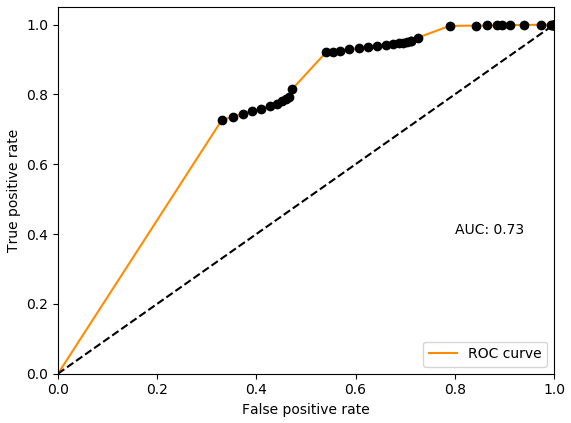
Figure A1The receiver operating characteristic (ROC) and area under curve (AUC) using the HEC-RAS as reference map against the water depth map derived from surface water interpolation.
This work relied on data which are available upon request from the providers cited in Sects. 2 and 3.
LW, HdM, MdR, AC and MvdH conceived the study. LW developed the theoretical framework and methodology with supervision from HdM, MdR, AC and MvdH. AK assisted in extracting and processing SAR data and helped LW carry out the inundation modeling. LW analyzed the data and prepared the draft, with all co-authors providing critical feedback and helping shape the analysis and manuscript.
The authors declare that they have no conflict of interest.
Publisher's note: Copernicus Publications remains neutral with regard to jurisdictional claims in published maps and institutional affiliations.
The authors would like to thank Jurg Wilbrink (510) and Gumbi Gumbi and Simon Tembo from the Malawi Red Cross Society data team for obtaining the UAV data and Thirza Teule for collecting the essential field observations. The first and second European Civil Protection and Humanitarian Aid Operation (ECHO) programs on resilience building in Malawi financed the UAV mission. We also thank the two anonymous reviewers for their valuable comments that helped improve the manuscript.
This research has been supported by the Dutch Research Council (NWO) (VIDI; grant no. 016.161.324).
This paper was edited by Sven Fuchs and reviewed by two anonymous referees.
Ai, J., Zhang, C., Chen, L., and Li, D.: Mapping Annual Land Use and Land Cover Changes in the Yangtze Estuary Region Using an Object-Based Classification Framework and Landsat Time Series Data, Sustainability, 12, 659, https://doi.org/10.3390/su12020659, 2020.
Alam, A., Bhat, M. S., Farooq, H., Ahmad, B., Ahmad, S., and Sheikh, A. H.: Flood risk assessment of Srinagar city in Jammu and Kashmir, India, International Journal of Disaster Resilience in the Built Environment, 9, 114–129, https://doi.org/10.1108/IJDRBE-02-2017-0012, 2018.
Amirebrahimi, S., Rajabifard, A., Mendis, P., and Ngo, T.: A framework for a microscale flood damage assessment and visualization for a building using BIM–GIS integration, Int. J. Digit. Earth, 9, 363–386, https://doi.org/10.1080/17538947.2015.1034201, 2016.
Belgiu, M. and Draguţ, L.: Comparing supervised and unsupervised multiresolution segmentation approaches for extracting buildings from very high resolution imagery, ISPRS J. Photogramm., 96, 67–75, https://doi.org/10.1016/j.isprsjprs.2014.07.002, 2014.
Blanco-Vogt, Á., Haala, N., and Schanze, J.: Building parameters extraction from remote-sensing data and GIS analysis for the derivation of a building taxonomy of settlements – a contribution to flood building susceptibility assessment, International Journal of Image and Data Fusion, 6, 22–41, https://doi.org/10.1080/19479832.2014.926296, 2015.
Blaschke, T.: Object based image analysis for remote sensing, ISPRS J. Photogramm., 65, 2–16, https://doi.org/10.1016/j.isprsjprs.2009.06.004, 2010.
Budiyono, Y., Aerts, J., Brinkman, J., Marfai, M. A., and Ward, P.: Flood risk assessment for delta mega-cities: A case study of Jakarta, Nat. Hazards, 75, 389–413, https://doi.org/10.1007/s11069-014-1327-9, 2015.
CAPRA: Probabilistic Risk Assessment Program, ERN-Vulnerability v2, available at: https://ecapra.org/ (last access: 8 May 2019), 2012.
Cian, F., Marconcini, M., Ceccato, P., and Giupponi, C.: Flood depth estimation by means of high-resolution SAR images and lidar data, Nat. Hazards Earth Syst. Sci., 18, 3063–3084, https://doi.org/10.5194/nhess-18-3063-2018, 2018.
CIESIN.: Facebook Connectivity Lab and Center for International Earth Science Information Network. High Resolution Settlement Layer (HRSL), Center for International Earth Science Information Network, available at: https://www.ciesin.columbia.edu/data/hrsl/ (last access: 21 April 2019), 2016.
Cohen, S., Brakenridge, G. R., Kettner, A., Bates, B., Nelson, J., McDonald, R., Huang, Y.-F., Munasinghe, D., and Zhang, J.: Estimating Floodwater Depths from Flood Inundation Maps and Topography, J. Am. Water Resour. As., 54, 847–858. https://doi.org/10.1111/1752-1688.12609, 2018.
Copier, W., de Ruiter, M. C., de Moel, H., Couasnon, A. A., and Teklesadik, A.: The impact of drone data on hydraulic modelling – A case study for an area in Malawi, Vrije Universiteit Amsterdam, Amsterdam, 2019.
De Angeli, S., Dell'Acqua, F., and Trasforini, E.: Application of an Earth-Observation-based building exposure mapping tool for flood damage assessment, E3S Web Conf., 7, 05001, https://doi.org/10.1051/e3sconf/20160705001, 2016.
de Moel, H. and Aerts, J. C. J. H.: Effect of uncertainty in land use, damage models and inundation depth on flood damage estimates, Nat. Hazards, 58, 407–425, https://doi.org/10.1007/s11069-010-9675-6, 2011.
de Moel, H., Asselman, N. E. M., and Aerts, J. C. J. H.: Uncertainty and sensitivity analysis of coastal flood damage estimates in the west of the Netherlands, Nat. Hazards Earth Syst. Sci., 12, 1045–1058, https://doi.org/10.5194/nhess-12-1045-2012, 2012.
de Moel, H., Jongman, B., Kreibich, H., Merz, B., Penning-Rowsell, E., and Ward, P. J.: Flood risk assessments at different spatial scales, Mitig. Adapt. Strat. Gl., 20, 865–890, https://doi.org/10.1007/s11027-015-9654-z, 2015.
de Ruiter, M. C., Ward, P. J., Daniell, J. E., and Aerts, J. C. J. H.: Review Article: A comparison of flood and earthquake vulnerability assessment indicators, Nat. Hazards Earth Syst. Sci., 17, 1231–1251, https://doi.org/10.5194/nhess-17-1231-2017, 2017.
Díaz-Delgado, C. and Gaytán Iniestra, J.: Flood Risk Assessment in Humanitarian Logistics Process Design, J. Appl. Res. Technol., 12, 976–984, https://doi.org/10.1016/S1665-6423(14)70604-2, 2014.
Englhardt, J., de Moel, H., Huyck, C. K., de Ruiter, M. C., Aerts, J. C. J. H., and Ward, P. J.: Enhancement of large-scale flood risk assessments using building-material-based vulnerability curves for an object-based approach in urban and rural areas, Nat. Hazards Earth Syst. Sci., 19, 1703–1722, https://doi.org/10.5194/nhess-19-1703-2019, 2019.
Farr, T. G. and Kobrick, M.: Shuttle radar topography mission produces a wealth of data, Eos, 81, 583, https://doi.org/10.1029/EO081i048p00583, 2000.
Fekete, A.: Spatial disaster vulnerability and risk assessments: Challenges in their quality and acceptance, Nat. Hazards, 61, 1161–1178, https://doi.org/10.1007/s11069-011-9973-7, 2012.
Government of Malawi: 2015 Floods Post Disaster Needs Assessment Report – Malawi, Government of Malawi, available at: https://reliefweb.int/report/malawi/malawi-2015-floods-post-disaster-needs-assessment-report (last access: 26 May 2019), 2015.
Grizonnet, M., Michel, J., Poughon, V., Inglada, J., Savinaud, M., and Cresson, R.: Orfeo ToolBox: Open-source processing of remote sensing images, Open Geospatial Data, Software and Standards, 2, 15, https://doi.org/10.1186/s40965-017-0031-6, 2017.
Gutierrez, I., Før Gjermundsen, E., Harcourt, W. D., Kuschnerus, M., Tonion, F., and Zieher, T.: Analysis of filtering techniques for investigating landslide-induced topographic changes in the oetz valley (Tyrol, Austria), ISPRS Annual Photogrammetry Remote Sensing and Spatial Information Sciences, V-2-2020, 719–726, https://doi.org/10.5194/isprs-annals-V-2-2020-719-2020, 2020.
Hosmer, D. W. and Lemeshow, S.: Applied logistic regression, Second edition, John Wiley and Sons Inc., USA, New York, 2000.
Hydrologic Engineering Center: HEC-RAS, River Analysis System User's Manual, Version 3.1, Davis, California, 1998.
IFRC: Malawi Floods: Emergency Plan of Action (EPoA), International Federation of Red Cross And Red Crescent Societies, available at: https://reliefweb.int/sites/reliefweb.int/files/resources/MDRMW014do.pdf, last access: 5 April 2019.
Jones, B.: Managing Post-Disaster Needs Assessments (PDNA), Managing Post-Disaster Needs Assessments (PDNA), World Bank, Washington, DC., EAP DRM Knowledge Notes, 19, 8, 2010.
Jongman, B., Kreibich, H., Apel, H., Barredo, J. I., Bates, P. D., Feyen, L., Gericke, A., Neal, J., Aerts, J. C. J. H., and Ward, P. J.: Comparative flood damage model assessment: towards a European approach, Nat. Hazards Earth Syst. Sci., 12, 3733–3752, https://doi.org/10.5194/nhess-12-3733-2012, 2012.
Kamps, M., Bouten, W., and Seijmonsbergen, A. C.: LiDAR and Orthophoto Synergy to optimize Object-Based Landscape Change: Analysis of an Active Landslide, Remote Sens., 9, 805, https://doi.org/10.3390/rs9080805, 2017.
Ke, Q., Jonkman, S. N., Van Gelder, P. H. a. J. M., and Rijcken, T.: Flood damage estimation for downtown Shanghai sensitivity analysis. Conference of the International Society for Integrated Disaster Risk Management IDRiM 2012, Authors Version: International Society for Integrated Disaster Risk Management, Beijing, China, available at: https://repository.tudelft.nl/islandora/object/uuid%3Abf75cdab-8a0d-4dbf-ae8e-61f59d3e5d86 (last access: 21 May 2019), 2012.
Klemas, V. V.: Coastal and Environmental Remote Sensing from Unmanned Aerial Vehicles: An Overview, J. Coastal Res., 31, 1260–1267, https://doi.org/10.2112/JCOASTRES-D-15-00005.1, 2015.
Koks, E. E., Bočkarjova, M., de Moel, H., and Aerts, J. C. J. H.: Integrated Direct and Indirect Flood Risk Modeling: Development and Sensitivity Analysis, Computat. Studies, 35, 882–900, https://doi.org/10.1111/risa.12300, 2015.
Maiti, S.: Defining a Flood Risk Assessment Procedure using Community Based Approach with Integration of Remote Sensing and GIS, International Institute for Geo-information Science and Earth Observation, Enschede, 2007.
Malawi Statistical Office: Fourth Integrated Household Survey (IHS4) 2016–2017, Ministry of Economic Planning and Development (MoEPD), Zomba, 2017.
Malgwi, M. B., Fuchs, S., and Keiler, M.: A generic physical vulnerability model for floods: review and concept for data-scarce regions, Nat. Hazards Earth Syst. Sci., 20, 2067–2090, https://doi.org/10.5194/nhess-20-2067-2020, 2020.
Malgwi M. B., Schlögl, M. and Keiler, M.: Expert-based versus data-driven flood damage models: A comparative evaluation for data-scarce regions, Int. J. Disast. Risk Re., 57, 102148, ISSN 2212-4209, https://doi.org/10.1016/j.ijdrr.2021.102148, 2021.
Mallupattu, P. K. and Sreenivasula Reddy, J. R.: Analysis of Land Use/Land Cover Changes Using Remote Sensing Data and GIS at an Urban Area, Tirupati, India, Sci. World J., 2013, e268623, https://doi.org/10.1155/2013/268623, 2013.
McVittie, A.: Sentinel-1 Flood mapping tutorial, Skywatch, ESA, available at: http://step.esa.int/docs/tutorials/tutorial_s1floodmapping.pdf (last access: 26 April 2019), 2019.
Merz, B., Kreibich, H., Thieken, A., and Schmidtke, R.: Estimation uncertainty of direct monetary flood damage to buildings, Nat. Hazards Earth Syst. Sci., 4, 153–163, https://doi.org/10.5194/nhess-4-153-2004, 2004.
Merz, B., Kreibich, H., Schwarze, R., and Thieken, A.: Review article ”Assessment of economic flood damage”, Nat. Hazards Earth Syst. Sci., 10, 1697–1724, https://doi.org/10.5194/nhess-10-1697-2010, 2010.
Michel, J., Youssefi, D., and Grizonnet, M.: Stable Mean-Shift Algorithm and Its Application to the Segmentation of Arbitrarily Large Remote Sensing Images, IEEE T. Geosci. Remote, 53, 952–964, https://doi.org/10.1109/TGRS.2014.2330857, 2015.
Mountrakis, G., Im, J., and Ogole, C.: Support vector machines in remote sensing: A review, ISPRS J. Photogramm., 66, 247–259, https://doi.org/10.1016/j.isprsjprs.2010.11.001, 2011.
Mouratidis, A. and Sarti, F.: Flash-Flood Monitoring and Damage Assessment with SAR Data: Issues and Future Challenges for Earth Observation from Space Sustained by Case Studies from the Balkans and Eastern Europe, in: Earth Observation of Global Changes (EOGC), edited by: Krisp, J. M., Meng, L., Pail, R., and Stilla, U., 125–136, Springer, Berlin, Heidelberg, https://doi.org/10.1007/978-3-642-32714-8_8, 2013.
Murnane, R. J., Daniell, J. E., Schäfer, A. M., Ward, P. J., Winsemius, H. C., Simpson, A., Tijssen, A., and Toro, J.: Future scenarios for earthquake and flood risk in Eastern Europe and Central Asia, Earth's Future, 5, 693–714, https://doi.org/10.1002/2016EF000481, 2017.
Nowak Da Costa, J., Calka, B., and Bielecka, E.: Urban Population Flood Impact Applied to a Warsaw Scenario, Resources, 10, 62, https://doi.org/10.3390/resources10060062, 2021.
OpenStreetMap contributors.: © OpenStreetMap, available at: https://www.openstreetmap.org, last access: 2 July 2019.
Rudari, R., Beckers, J., De Angeli, S., Rossi, L., and Trasforini, E.: Impact of modelling scale on probabilistic flood risk assessment: the Malawi case, 3rd European Conference on Flood Risk Management (FLOODrisk 2016), Savona, Italy, https://doi.org/10.1051/e3sconf/20160704015, 2016.
Saint-Geours, N., Lavergne, C., Bailly, J.-S., and Grelot, F.: Ranking sources of uncertainty in flood damage modelling: A case study on the cost-benefit analysis of a flood mitigation project in the Orb Delta, France, J. Flood Risk Manag., 8, 161–176, https://doi.org/10.1111/jfr3.12068, 2015.
Shen, X., Wang, D., Mao, K., Anagnostou, E., and Hong, Y.: Inundation Extent Mapping by Synthetic Aperture Radar: A Review., Remote Sens., 11, 879, https://doi.org/10.3390/rs11070879, 2019.
SNAP: European Space Agency Sentinel Application Platform v6.0, ESA, available at: http://step.esa.int, last access: 5 June 2019.
Starkey, E., Parkin, G., Birkinshaw, S., Large, A., Quinn, P., and Gibson, C.: Demonstrating the value of community-based (“citizen science”) observations for catchment modelling and characterisation, J. Hydrol., 548, 801–817, https://doi.org/10.1016/j.jhydrol.2017.03.019, 2017.
Teule, T., Couasnon, A., Bischiniotis, K., Blasch, J., and van den Homberg, M.: Towards improving a national flood early warning system with global ensemble flood predictions and local knowledge; a case study on the Lower Shire Valley in Malawi., EGU General Assembly 2020, Online, 4–8 May 2020, EGU2020-507, https://doi.org/10.5194/egusphere-egu2020-507, 2019.
Trogrlić, R., Wright, G., Adeloye, A., Duncan, M., and Mwale, F.: Community based-flood risk management: experiences and challenges in Malawi, Conference: XVI World Water Congress, 29 May–3 June, Abstract number 173, Cancun, Mexico, 2017.
UNDRR: Global Assessment Report on Disaster Risk Reduction, United Nation office of Disaster Risk Reduction, Geneva, 2019.
van den Homberg, M. and Susha, I.: Characterizing Data Ecosystems to Support Official Statistics with Open Mapping Data for Reporting on Sustainable Development Goals, ISPRS Int. J. Geo-Inf., 7, 456, https://doi.org/10.3390/ijgi7120456, 2018.
van den Homberg, M. J. C., Wilbrink, J., Crince, A., Kersbergen, D., Gumbi, G., Tembo, S., and Lemmens, R.: Combining UAV Imagery, Volunteered Geographic Information, and Field Survey Data to Improve Characterization of Rural Water Points in Malawi, ISPRS Int. J. Geo-Inf., 9, 592, https://doi.org/10.3390/ijgi9100592, 2020.
Wagenaar, D. J., de Bruijn, K. M., Bouwer, L. M., and de Moel, H.: Uncertainty in flood damage estimates and its potential effect on investment decisions, Nat. Hazards Earth Syst. Sci., 16, 1–14, https://doi.org/10.5194/nhess-16-1-2016, 2016.
Winter, B., Schneeberger, K., Huttenlau, M., and Stötter, J.: Sources of uncertainty in a probabilistic flood risk model, Nat. Hazards, 91, 431–446, https://doi.org/10.1007/s11069-017-3135-5, 2019.
Xu, L., Jing, W., Song, H., and Chen, G.: High-Resolution Remote Sensing Image Change Detection Combined With Pixel-Level and Object-Level, IEEE Access, 7, 78909–78918, https://doi.org/10.1109/ACCESS.2019.2922839, 2019.
Zeybek, M. and Şanlıoğlu, İ.: Point Cloud Filtering on UAV Based Point Cloud, Measurement, 133, 99–111, https://doi.org/10.1016/j.measurement.2018.10.013, 2019.