the Creative Commons Attribution 4.0 License.
the Creative Commons Attribution 4.0 License.
 | 13 Oct 2021
Residential building stock modelling for mainland China targeted for seismic risk assessment
James Edward Daniell
Hing-Ho Tsang
Friedemann Wenzel
To enhance the estimation accuracy of economic loss and casualty in seismic risk assessment, a high-resolution building exposure model is necessary. Previous studies in developing global and regional building exposure models usually use coarse administrative-level (e.g. country or sub-country level) census data as model inputs, which cannot fully reflect the spatial heterogeneity of buildings in large countries like China. To develop a high-resolution residential building stock model for mainland China, this paper uses finer urbanity-level population and building-related statistics extracted from the records in the tabulation of the 2010 population census of the People's Republic of China (hereafter abbreviated as the “2010 census”). In the 2010 census records, for each province, the building-related statistics are categorized into three urbanity levels (urban, township, and rural). To disaggregate these statistics into high-resolution grid level, we need to determine the urbanity attributes of grids within each province. For this purpose, the geo-coded population density profile (with 1 km × 1 km resolution) developed in the 2015 Global Human Settlement Layer (GSHL) project is selected. Then for each province, the grids are assigned with urban, township, or rural attributes according to the population density in the 2015 GHSL profile. Next, the urbanity-level building-related statistics can be disaggregated into grids, and the 2015 GHSL population in each grid is used as the disaggregation weight. Based on the four structure types (steel and reinforced concrete, mixed, brick and wood, other) and five storey classes (1, 2–3, 4–6, 7–9, ≥10) of residential buildings classified in the 2010 census records, we reclassify the residential buildings into 17 building subtypes attached with both structure type and storey class and estimate their unit construction prices. Finally, we develop a geo-coded 1 km × 1 km resolution residential building exposure model for 31 provinces of mainland China. In each 1 km × 1 km grid, the floor areas of the 17 residential building subtypes and their replacement values are estimated. The model performance is evaluated to be satisfactory, and its practicability in seismic risk assessment is also confirmed. Limitations of the proposed model and directions for future improvement are discussed. The whole modelling process presented in this paper is fully reproducible, and all the modelled results are publicly accessible.
- Article
(12270 KB) - Full-text XML
- BibTeX
- EndNote


The frequent occurrence of earthquakes and other natural hazards (typhoon, flood, tsunami, etc.) can lead to tremendous and often crippling economic losses. According to the estimation in Daniell et al. (2017), from 1900–2016, 2.3 million earthquake fatalities from 2233 fatal events occurred worldwide. Economic losses (direct and indirect) associated with the occurrence of over 9900 damaging earthquakes reached USD 3.41 trillion (in 2016 prices). For cases in China, the combination of high seismic activity, population density, and building vulnerability caused even higher seismic risk: earthquakes that occurred in China during the 110 years from 1900 to 2010 accounted for about 2.5 % of radiated energy globally, but the earthquake fatality ratio is around of the world (Wu et al., 2013). Among the losses caused by natural disasters, buildings are considered to be the most important asset category since the main sources of loss and fatality that occur during earthquakes are related to building damage and collapse (e.g. Neumayer and Barthel, 2011; Yuan, 2008). Information on the exposed value of buildings is key to seismic loss estimation, whose accuracy will further affect the effectiveness in earthquake response and rescue (Xu et al., 2016a). Therefore, in any seismic risk mitigation effort, the estimation of the building stock and the values at risk should be given top priority. This is even more urgent for seismic active and disaster vulnerable countries like China (Allen et al., 2009), where rapid urbanization has led to a massive increase in both the asset value and population that are exposed to a potential seismic hazard (Hu et al., 2010; Yang and Kohler, 2008).
Modelling seismic loss to buildings requires quantifying their exposure in terms of floor area and monetary value (Paprotny et al., 2020). A series of micro-, meso-, and macro-scale approaches have been developed for this purpose. The scale of the method depends not only on the size of the study area but also on the goal of the investigation, the availability of necessary data, time, money, and human resources (Messner and Meyer, 2006). For example, micro-scale analyses calculate the asset value based on individual buildings, which requires detailed information on building characteristics (e.g. occupancy, age, structure type, building height, or the number of floors). However, since great efforts and considerable expenses are required to collect such information for each building, micro-scale methods are rarely applicable on a regional or (inter)national level (e.g. Figueiredo and Martina, 2016; Erdik, 2017). When further limited by the privacy protection issue, information on asset values of individual buildings is more difficult to obtain (Wünsch et al., 2009). In contrast, meso- and macro-scale methods that use aggregated exposure data on building characteristics procured from official statistics and organized in administrative units (e.g. country, province, prefecture, county or district, etc.) are more commonly used in modelling building values exposed to future earthquakes.
Since building-related statistics are usually aggregated at a coarse administrative level, while seismic hazards are usually modelled with high spatial resolution, there is a spatial mismatch between exposure data and hazard mapping (e.g. Chen et al., 2004; Thieken et al., 2006). This mismatch may delay and mislead the recuse decision-making after large earthquakes. For example, after the occurrence of the Ms 8.0 Wenchuan earthquake, one of the most severely affected areas, Qingchuan County, did not get an appropriate rescue response, while most of the recuse resources were sent to the less damaged city of Dujiangyan. The major reason for this problem was that the exposure data (population, buildings) used to assess seismic loss were based on administrative units (Xu et al., 2016a). Therefore, to enhance seismic risk assessment accuracy, the aggregated building statistics data need to be spatialized into high-resolution grid levels. Several interpolation and decomposition methods (e.g. areal weighting, pycnophylactic interpolation, dasymetric mapping) have been developed for this purpose. Compared with the areal weighting method, in which the aggregated building data are evenly distributed (e.g. Goodchild et al., 1993), the pycnophylactic interpolation method uses a smoothing function of distance to determine the disaggregation weight (e.g. Tobler, 1979) and tends to be more reasonable since the distribution of buildings within an administrative unit is heterogeneous. Based on the pycnophylactic interpolation method, the dasymetric mapping method (Bhaduri et al., 2007) further utilizes finer-resolution ancillary spatial data to augment the interpolation process and is now widely used.
When using the dasymetric mapping method to spatialize the administrative-level building exposure data, the selection of appropriate ancillary information is thought to be the most difficult part (Wu et al., 2018) since such information should not only be geo-coded and readily available but also have a high correlation with the building exposure data to be disaggregated. A range of remote sensing data (e.g. nightlight data, road density, land use and land type, population spatial distribution datasets, etc.) have been employed as ancillary information in the literature. A detailed summary of these ancillary data are given in the “Data sources and methodology” section.
Based on the aggregated building-related statistics and using the dasymetric mapping method, this paper develops a high-resolution residential building model (in terms of building floor area and replacement value) for seismic risk assessment in mainland China. This issue has been explored in many previous studies, and a series of global and regional building exposure models have been developed. One famous global model is the PAGER (Prompt Assessment of Global Earthquakes for Response) building inventory database, which is the first open, publicly available, transparently developed global model (Jaiswal et al., 2010). However, the PAGER inventory was developed to rapidly estimate human occupancies in different structure types for earthquake fatality assessment. It lacks information in actual building counts and does not use available information from a commercial database or remote sensing data and thus cannot be used for building asset evaluation immediately (Dell'Acqua et al., 2013). To overcome this difficulty, at least partially, the GED4GEM (the Global Exposure Database for the Global Earthquake Model) project develops a complementary approach that can provide a spatial inventory of exposed assets for catastrophe modelling and loss estimation worldwide (Gamba, 2014). The input datasets ingested into the GED4GEM are at multiple spatial scales, from coarse country-level statistics to finer compilations of each building in some sample regions. There are also other global models, such as the series of building stock models released by the Global Assessment Report (De Bono and Chatenous, 2015; De Bono and Mora, 2014; De Bono et al., 2013) of the United Nations International Strategy for Disaster Reduction (UNISDR) and the global exposure dataset created by Gunasekera et al. (2015). When focusing on the modelling of building stock in China, a common limitation shared by these global models is that the building-related statistics they disaggregate are only of country or sub-country level, although finer-level statistics are already available. Thus, a general assumption in the disaggregation process of these global models is that building stock value per capita within the country or sub-country is uniform. A similar assumption is also made in studies that develop building exposure models specifically for China (e.g. Yang and Kohler, 2008; Hu et al., 2010). For computational convenience, such an assumption is acceptable. However, for improving the seismic risk assessment accuracy in each specific country, more detailed aggregated data at a finer level, if available, should be fully employed in the development of their building exposure model.
By considering the depreciation of all physical fixed assets (including residential and non-residential buildings, infrastructures, tools, machinery, and equipment), Wu et al. (2014) estimated the wealth capital stock (WKS) value for 344 prefectures in mainland China using the perpetual inventory method (PIM). Later, Wu et al. (2018) decomposed the prefecture-level WKS value into building assets, infrastructure assets, and other assets with fixed percentage shares of 44 %, 19 %, and 37 % for all 344 prefectures. And these three asset components were further disaggregated into 800 m × 800 m high-resolution grids by using LandScan population, road density, and nighttime light as ancillary information, respectively. The basic idea of combining the use of different ancillary information to disaggregate the WKS value in Wu et al. (2018) is good. However, the oversimplification in fixing the percentage shares of the building, infrastructure, and other assets in all prefectures limits the applicability of their results in actual seismic risk assessment.
Based on the county-level building-related statistics extracted from the 2010 census records, Xu et al. (2016b) developed the nation-wide dasymetric foundation data (including population and buildings) for quick earthquake disaster loss assessment and emergency response in China by using the multivariate regression method (Xu et al., 2016a). The multivariate regression method used in Xu et al. (2016a) was explained in more detail by Chen et al. (2012) and Han et al. (2013), in which they developed the population and building exposure models for areas in Yunnan Province. Fu et al. (2014a) also used the multivariate regression method to produce the 1 km × 1 km resolution population grids in the years 2005 and 2010 for mainland China. Important assumptions in this multivariate regression method are that (1) the spatial distribution of population is limited within the six land use types (namely cultivated land, forest land, grass land, rural residential land, urban residential land, industrial and transportation land) recognized from the Landsat Thematic Mapper (TM) images, and (2) for counties with similar geographical and demographic characteristics (e.g. population number, structure, and economy development level), the population density within each land use type is the same. Recently, Lin et al. (2020) conducted a township- and street-level comparison of population models generated by Fu et al. (2014a) and other institutes for Guangdong Province, China, with the surveyed population in 2010 census records. Their comparison shows that the township- and street-level population generated by using the multivariate regression method in Fu et al. (2014a) tends to overpredict the population density in a sparsely populated area and underpredict the population density in a densely populated area, especially the downtown area of metropolitan cities like Shenzhen and Guangzhou. The reasons for such discrepancies are that (1) the population density developed for each land use type by using the multivariate regression method is the average population density (thus the over- or underprediction of the actual population density in certain areas is inevitable), and (2) when applying the multivariate regression method, no additional supplementary data (e.g. road density, nighttime light) are employed to adjust the level of development in different regions, which is necessary because the level of development is much higher than the average in places such as the downtown area of metropolitan cities like Shenzhen and Guangzhou. Although the building exposure model developed by Xu et al. (2016b) has not yet been tested, we conclude that the model of Xu et al. (2016b) also suffers from the over- or underprediction problem in Fu et al. (2014a).
To overcome the limitations in building exposure models developed for mainland China in previous studies, this paper aims to present an improved method for generating a high-resolution residential building stock model (in terms of building floor area and replacement value) for mainland China. The main improvements in this paper are that (1) compared with global building exposure models, we use finer urbanity-level (urban, township, and rural) building-related statistics extracted from the 2010 census records as model inputs; (2) compared with Wu et al. (2018), in which the building assets are decomposed from the composite WKS value with a fixed percentage share for all prefectures, we use statistics that are directly related to residential buildings for each urbanity level of each province; and (3) compared with Xu et al. (2016b), in which only land use data are employed in the multivariate method to derive the average building floor area density within each grid, we use the ancillary population density profile generated from the 2015 Global Human Settlement Layer (GHSL), which is considered to be the best available assessment of spatial extents of human settlements with unprecedented spatiotemporal coverage and detail (e.g. Freire et al., 2016).
The organization of the paper is as follows. Section 2 (“Data sources and methodology”) firstly describes the building-related statistics to be used as model inputs that were extracted from the 2010 census records (Sect. 2.1), the review and selection of ancillary data to disaggregate these statistics into grid level (Sect. 2.2), and the derivation of residential building floor area and replacement value in each grid based on these statistics and the ancillary data (Sect. 2.3 and 2.4). Then the major results are presented (Sect. 3.1), and comparisons with other independent data sources are conducted (Sect. 3.2). Limitations in this paper and further improvement directions are also discussed in Sect. 4. Conclusions are drawn in Sect. 5.
In dasymetric mapping, the use of finer-scale census data as input and the choice of appropriate ancillary remote sensing data to disaggregate the census data into a higher grid level are the two controlling factors for the quality of the building stock model. For China, after the 2010 sixth population census (namely the 2010 census), detailed statistical data related to residential building characteristics (e.g. building occupancy, structure type, height classes, etc.) are available for each province at the urbanity level (urban, township, rural). These urbanity-level building-related statistics are good data sources to develop the building exposure model for China. To disaggregate these statistics into grid level, the correlation between the ancillary remote sensing data and the building-related statistics needs to be established. Then, the building floor area and replacement value at the grid level can be estimated. Therefore, in this section we introduce the residential-building-related statistics as extracted from the 2010 census records, the review and selection of ancillary remote sensing data to disaggregate these statistics into grid level, and the method to derive the grid-level residential building floor area and replacement value based on these statistics and the ancillary remote sensing data.
2.1 The building-related statistics in the 2010 census records
The statistics to be used in this paper for building stock modelling are extracted from the tabulation of the 2010 population census of the People's Republic of China (namely the 2010 census), particularly for residential buildings. Like in most countries of the world, the nation-wide population and housing census in China is carried out in 10-year intervals. Detailed statistics for the year 2020 are not publicly accessible yet. Therefore, census data for the year 2010 are used to elaborate the modelling process. In the 2010 census, there are two types of tables: long table and short table. The long table includes summaries based on the surveys of 10 % of the total population in mainland China, while the short table summaries are based on the surveys of the whole population. Statistics on building characteristics (e.g. building occupancy type, height classes, structure type, etc.) are extracted from the long table of the 2010 census. Supplementary demographic statistics (e.g. the total population in each urbanity, the average number of people per family, and average floor area per person) are extracted from the short table of the 2010 census. A detailed introduction of corresponding sources of these data is given in Table 1.
Table 1Main data sources used in this paper. Access to these data is provided in the “Code and data availability” section; n/a stands for not applicable.
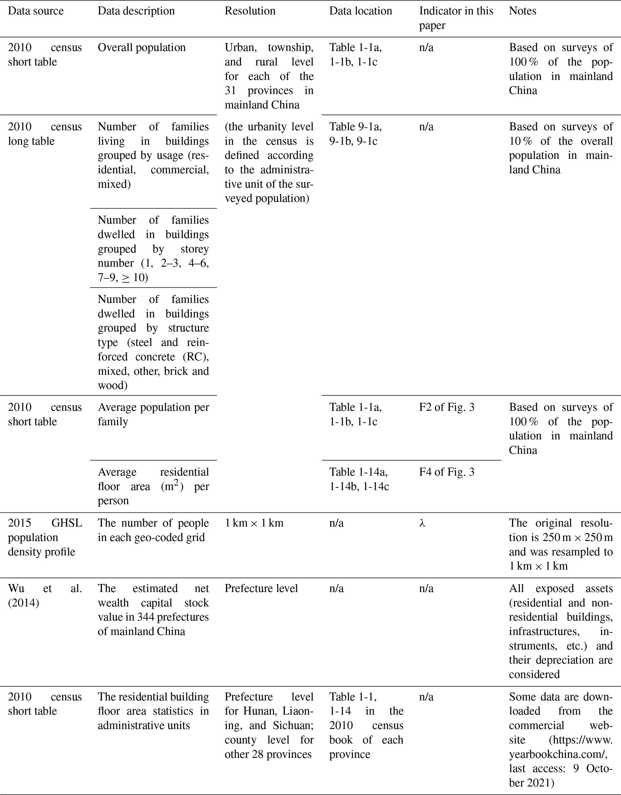
Note: the “2010 census” under “Data source” is the abbreviation of the “2010 Population Census of the People's Republic of China”; “Data location” refers to the serial number of the table in the original data source (see context in Sect. 2.1 for more details).
For each of the 31 provincial administrative units in mainland China (including five autonomous regions – Xinjiang, Tibet, Ningxia, Inner Mongolia, Guangxi – and four municipalities – Beijing, Shanghai, Tianjin, Chongqing, hereafter all referred to as provinces), statistics on building characteristics in the long table of the 2010 census are aggregated into three urbanity levels (urban, township, rural). The urbanity attribute is determined according to the administrative unit of the surveyed population. As listed in Table 2, these statistics are used as model inputs to develop the grid-level residential building model in terms of floor area and replacement value. Compared with country- and sub-country-level census data used in previous global or regional models, the further categorization of building-related statistics into urbanity level in the 2010 census helps differentiate the spatial heterogeneity of buildings within each province since the building-related statistics of the same urbanity level are from areas with similar development background but different administrative units. The spatial administrative boundaries used in this paper are from the National Geomatics Centre of China (see “Code and data availability” section for access).
Table 2In each urbanity, the population sum of the 2015 GHSL profile and the residential-building-related statistics extracted from the 2010 census records.
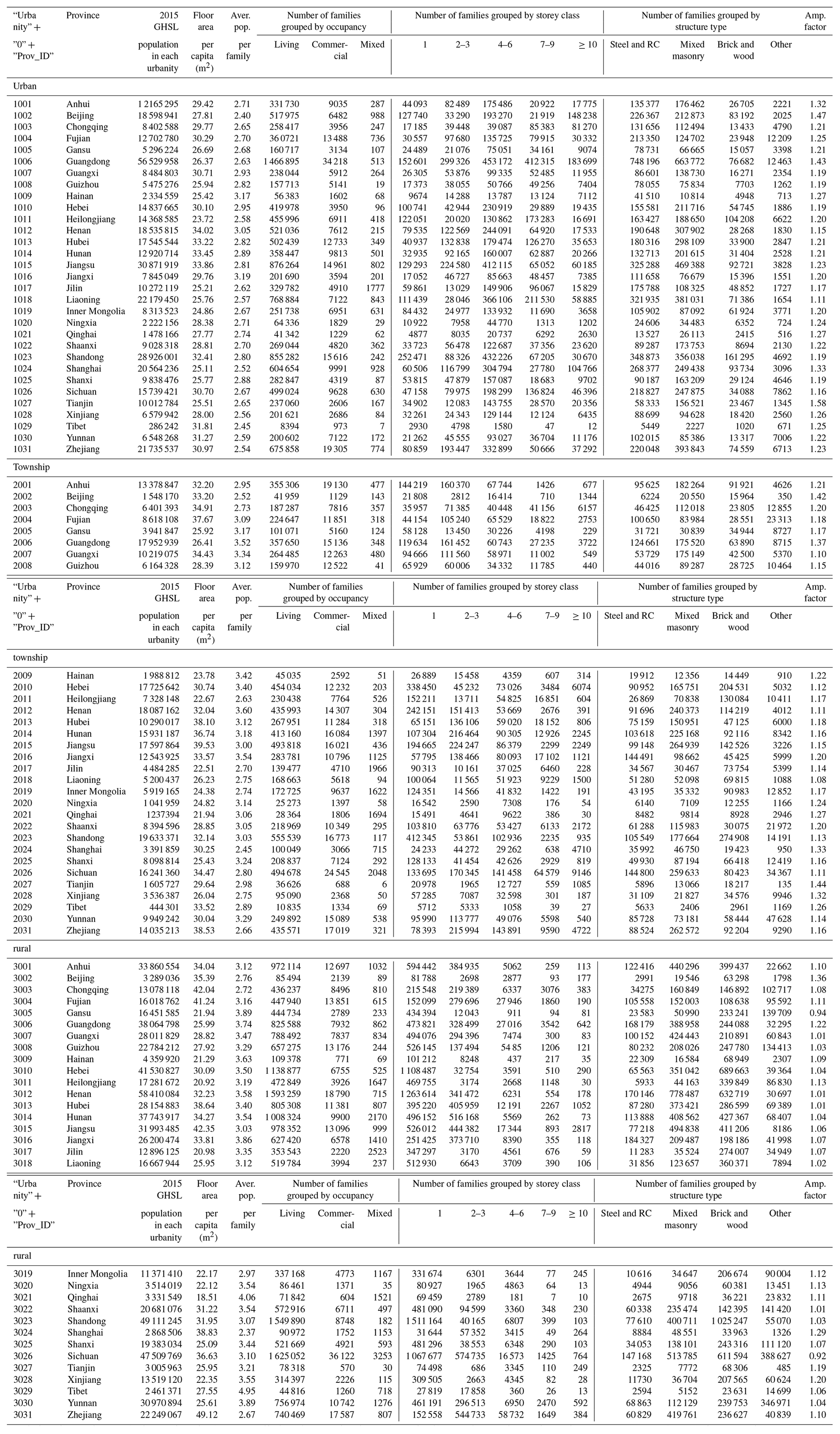
Note: the three urbanity attributes, namely urban, township, and rural, are represented by the numbers 1, 2, and 3 in the first column of this table; “Prov_id” refers to the ID number of each province; “Aver. pop. per family” refers to the average number of people per family; “Amp. factor” refers to the amplification factor used to amplify the building-related statistics from 2010 to 2015 (see Sect. 2.1 and 2.4.1 for more details).
2.2 Review and selection of ancillary remote sensing data for dasymetric building stock modelling
Before disaggregating the urbanity-level building-related statistics into 1 km × 1 km grid level, appropriate ancillary information needs to be carefully selected and evaluated. The use of remote sensing data as ancillary information to determine the disaggregation weight is common in dasymetric modelling and has been frequently adopted in previous studies (e.g. Aubrecht et al., 2013; Gunasekera et al., 2015; Silva et al., 2015). The most commonly used remote sensing data include land use and land cover (LULC) data (e.g. Eicher and Brewer, 2001; Wünsch et al., 2009; Seifert et al., 2010; Thieken et al., 2006), nighttime light data (e.g. Doll et al., 2006; Ghosh et al., 2010; Chen and Nordhaus 2011; Ma et al., 2012), and road density data (e.g. Gunasekera et al., 2015; Wu et al., 2018). According to Wu et al. (2018), the LULC, nighttime light, and road density data can be categorized as primary remote sensing data.
All primary remote sensing data have their pros and cons when used for dasymetric disaggregation. For example, studies using LULC data (e.g. Globcover, GLC2000, MODIS, GlobeLand30) assume that the population within each land-use type is uniformly distributed, which is a better assumption compared with believing in an evenly distributed population within an administrative unit. But this assumption is not consistent with the real situation (Thieken et al., 2006), specifically in suburban and rural areas, where the dispersion of population is greater than in urban areas (Bhaduri et al., 2007). Therefore, LULC data are inadequate to fully reflect the spatial heterogeneity within each land use or land cover class. In contrast, nighttime light data, acquired by the US Air Force Defense Meteorological Satellite Program (DMSP) Operational Linescan System (OLS) (Elvidge et al., 2007) and provided by the National Oceanic and Atmospheric Administration (NOAA) every year, are considered the most suitable ancillary information for indicating both the distribution and the density of human settlements and economic activities (Wu et al., 2018). Nighttime light data have been widely used to produce grid-based global population and GDP datasets (e.g. Ghosh et al., 2010; Chen and Nordhaus, 2011; Ma et al., 2012). However, the drawbacks of nighttime light intensity data are also obvious. Limited by the operating conditions of DMSP satellites, the range of nighttime light density is within a narrow interval of 0–63, thus leading to the pixel oversaturation in urban centres (Elvidge et al., 2007). For areas other than city centres (e.g. mountainous rural area), the coverage of nighttime light data is incomplete as it cannot correctly reflect the distribution of nonluminous objects (e.g. road transportation facilities, electricity infrastructure). Compared with the LULC and nighttime light data, road distribution data are more frequently used for assessing infrastructure assets since power lines, energy pipelines, water supply, and sewage pipelines are generally buried along the roads (Wu et al., 2018). Currently, road density data can be converted from road networks like OpenStreetMap, which is an openly available but crowdsourced online database (Zhang et al., 2015). As these data are not systematically compiled, there is still room for improvements (Wu et al., 2018).
Given the limitation of all primary remote sensing data, a series of secondary ancillary datasets are developed based on the combined use of these primary datasets. For example, the famous LandScan population density profile was produced by apportioning the best available census counts into cells based on probability coefficients, which were derived from road proximity, slope, land cover, and nighttime lights (Dobson et al., 2000). Based on these primary and secondary ancillary datasets, a series of studies have been conducted to disaggregate administrative-level building census data into geo-coded grids. For example, Silva et al. (2015) disaggregated the building stock at the parish level for mainland Portugal based on the population density profile at 30×30 arcsec resolution cells from LandScan. Gunasekara et al. (2015) developed an adaptive global exposure model (including three independent geo-referenced databases, namely building inventory stock, non-building infrastructure, and sector-based GDP), in which build-up area and LandScan population density are used to disaggregate country-level exposed asset value. Wu et al. (2018) established a high-resolution asset value map for mainland China by spatializing the prefecture-level depreciated capital stock value into grids using the combination of three ancillary datasets – nighttime light, LandScan population, and road density, to name just a few.
In this paper, we follow the assumption of Thieken et al. (2006) that the distribution of residential asset values can be directly reflected by population distribution. Now the remaining question is how to select appropriate ancillary population spatial distribution data to disaggregate building-related statistics in the 2010 census records. The candidate population datasets include Gridded Population of the World (GPW; Balk and Yetman, 2004), Global Rural–Urban Mapping Project (GRUMP) population (see “Code and data availability” section), LandScan (Bhaduri et al., 2007), WorldPop (Linard et al., 2012) or AsiaPop (Gaughan et al., 2013), PopGrid China (Fu et al., 2014b), Global Human Settlement Layer (GHSL) population grids (Freire et al., 2016; Pesaresi et al., 2013), etc. GPW is a product of simple areal weighting interpolation, and GRUMP is derived through simple dasymetric modelling, while LandScan is structurally a multidimensional dasymetric model (Bhaduri et al., 2007). According to Gunasekera et al. (2015), the LandScan gridded population dataset was identified as the best-suited dataset for exposure disaggregation, while other gridded population datasets such as GPW and GRUMP were too coarse in resolution and accuracy. According to Wu et al. (2018), LandScan, AsiaPop, and PopGrid China are the most promising population density datasets for asset value disaggregation in China since they all contain high-resolution attributes. However, some population data of China are missing from the current AsiaPop. And compared with LandScan, the spatial coverage of PopGrid China is limited, which is due to an assumption in its development method, namely the multivariate regression method (Fu et al., 2014a). It was assumed that the spatial distribution of population is limited to the six land use types recognized from the Landsat TM images, namely cultivated land, forest land, grass land, rural residential land, urban residential land, and industrial and transportation land. However, in reality, the population is distributed more widely beyond these land use types. Thus, the LandScan dataset was used for the final disaggregation of building assets in Gunasekera et al. (2015) and Wu et al. (2018). However, due to its commercial nature, the details to create the LandScan population datasets are less transparent, although it is considered to be one of the best global population density datasets (Sabesan et al., 2007). In contrast, the population datasets developed by the GHSL project of the Joint Research Center of the European Commission based on the global human settlement areas extracted from multi-scale textures and morphological features are transparent and freely available. The built-up area in GHSL was built by combining the MODIS 500 urban land cover (MODIS500) and the LandScan 2010 population layer and are among the best-known binary products based on remote sensing (Ji et al., 2020). Preliminary tests confirm that the quality of the information on built-up areas delivered by the GHSL is better than other available global information layers extracted by automatic processing of Earth observation data (Lu et al., 2013; Pesaresi et al., 2016). Furthermore, different from LandScan, which aims at representing the ambient population, namely the average population over a typical diurnal cycle (Elvidge et al., 2007), GHSL population grids represent the residential population in buildings (Corbane et al., 2017). The building-related statistics in the 2010 census are also for residential buildings. Therefore, the GHSL population grids are the best candidate ancillary information for this paper to disaggregate the urbanity-level building-related statistics extracted from the 2010 census records into grid level. The high correlation (R2=0.9662, as shown in Fig. 1) between the GHSL population and the 2010 census-recorded population at the county level further indicates its appropriateness. Detailed county-level population correlation analyses for each of the 31 provinces in mainland China are also provided and can be found from the Supplement online. The access to the remote sensing data mentioned above is provided in the “Code and data availability” section.

Figure 1County-level comparison of the population between the 2015 GHSL profile and the 2010 census records.
2.3 Assign urbanity attribute (urban, township, rural) to the geo-coded grids in the 2015 GHSL population density profile
In the 2015 GHSL population density profile, the number of people in each geo-coded grid is given (it is worth noting that this dataset has been updated in 2019 during the preparation of this work). The original resolution of the 2015 GHSL population density profile is 250 m × 250 m. For computational convenience, it is resampled to 1 km × 1 km resolution before further analysis. Based on the urbanity-level residential-building-related statistics extracted from the 2010 census records, a top-down dasymetric mapping method is performed to disaggregate the urbanity-level statistics into 1 km × 1 km resolution grids for mainland China. The urbanity attribute of statistics in the 2010 census records is determined according to the administrative unit of the surveyed population. For example, if a residence is from a village, then the related statistics are aggregated into rural urbanity level; if from a town, then it is township level; and if from a city, it is urban level. However, for the geo-coded population grids in the 2015 GHSL profile, the corresponding urbanity attributes remain to be defined. Therefore, before performing the disaggregation, we first define the urbanity attribute of each geo-coded grid in the 2015 GHSL profile by applying the reallocation approach developed by Aubrecht and Leon Torres (2015) and illustrated in Gunasekera et al. (2015).
Aubrecht and Leon Torres (2015) identify the geospatial areas of mixed and residential grids within the urban extent of the city of Cuenca, Ecuador, by using the Impervious Surface Area (ISA) data as they show strong spatial correlations with the built-up areas. The assumption behind their method was that intense lighting is associated with a high likelihood of commercial and/or industrial presence (which is commonly clustered in certain parts of a city, such as central business districts and/or peripheral commercial zones, and such areas are defined as “mixed-use area”), and areas of low light intensity are more likely to be pure residence zones (defined as “residential-use area”). In Gunasekera et al. (2015), a similar procedure was used in developing the building stock model for the entire globe. The difference is that Gunasekera et al. (2015) sorted the grids according to the population density in the LandScan population dataset and assigned the grid with urban or rural attributes. For each country, the largest and most populated contiguous grids are classified as urban. This step was repeated iteratively until the urban population proportion for each country was reached.
In this paper, to assign the urbanity attributes (namely urban, township, or rural) to geo-coded population grids in the 2015 GHSL profile, for each province we follow the urban, township, or rural population proportions (as listed in Table 3) derived from the population statistics in the short table of the 2010 census. The assumption behind this urbanity attribute assignment practice is that the larger the population density in a grid, the higher its potential to be assigned as “urban”. An example demonstrating the distribution of the 2015 GHSL population grids assigned with urban, township, and rural attributes for Baoshan District of Shanghai is shown in Fig. 2. For instance, in Shanghai, the urban, township, and rural population proportion derived from the 2010 census records is 76.64 %, 12.66 %, and 10.7 %, respectively. Then, following Gunasekera et al. (2015), the grids (1 km × 1 km) in the 2015 GHSL profile of Shanghai are sorted from the largest to the smallest in population density. The population in those most populated grids is selected and summed up until the urban population proportion (i.e. 76.64 % for Shanghai) is reached. Then those selected grids are assigned with the “urban” attribute, and the smallest population among these grids determines the threshold to divide urban and non-urban grids (for Shanghai this urban and non-urban grid population threshold is 4936/km2). For the remaining non-urban grids, the same process is repeated iteratively until the township population proportion (i.e. 12.66 % for Shanghai) is reached. These grids are assigned with the “township” attribute, and the smallest population among these grids determines the threshold to divide township and rural grids (for Shanghai this township and rural grid population threshold is 2750/km2). The remaining grids are thus assigned with the “rural” attribute. The urban and township as well as township and rural population thresholds for 31 provinces in mainland China are listed in Table 3. This process is repeated for all provinces.
Table 3The population proportions and thresholds used for each province to assign the grids in the 2015 GHSL profile with urban, township, or rural attributes.
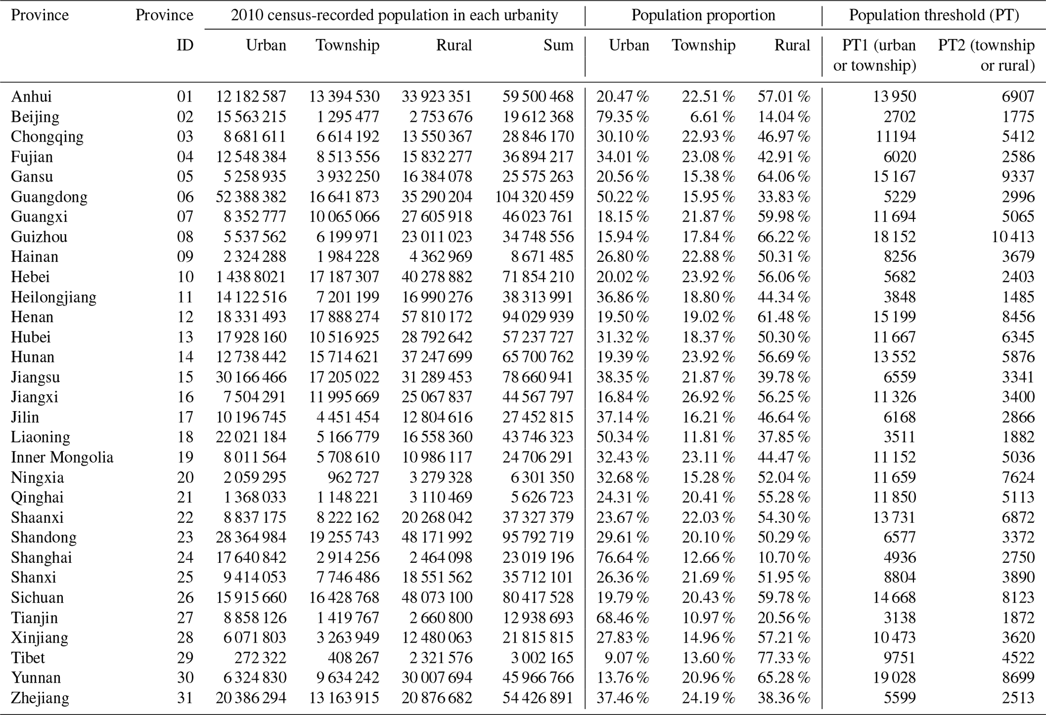
Note: for each province, “PT1(urban or township)” and “PT2 (township or rural)” are the population thresholds to assign the grids in the 2015 GHSL profile with urban, township, or rural attributes. According to the population density λ in each grid, the assignment criteria are that if λ≥ PT1, the grid is assigned as urban; if PT1 >λ≥ PT2, the grid is assigned as township; if λ< PT2, the grid is assigned as rural (see context in Sect. 2.3 for more details).
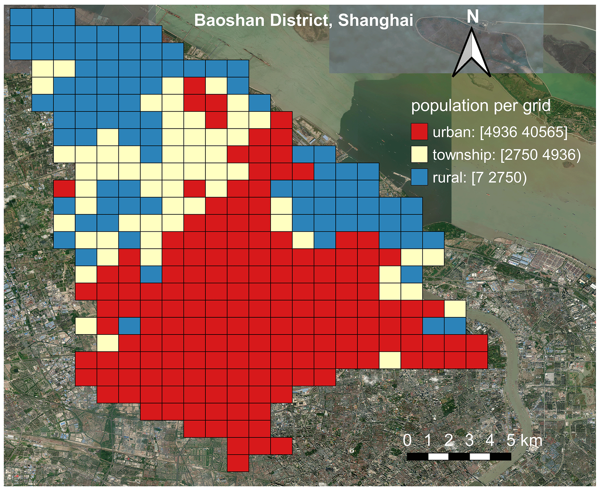
Figure 2An example showing the assignment of urbanity attribute in the 2015 GHSL population grids for Baoshan District in Shanghai. The urban and township as well as township and rural population thresholds for Shanghai are 4936/km2 and 2750/km2, respectively (see context in Sect. 2.3 for more details). This figure is plotted by using the QGIS platform (https://qgis.org/en/site/, last access: 9 October 2021), and the background satellite map is provided by the Bing map service (© Microsoft).
2.4 Residential building stock modelling process
The following section introduces the key steps in residential building stock modelling, including the disaggregation of urbanity-level statistics extracted from the 2010 census records into grid level, the reclassification of building subtypes with both structure type and storey class, and the derivation of residential building floor area and replacement value in each grid. The flowchart in Fig. 3 gives an overview of the whole modelling process.
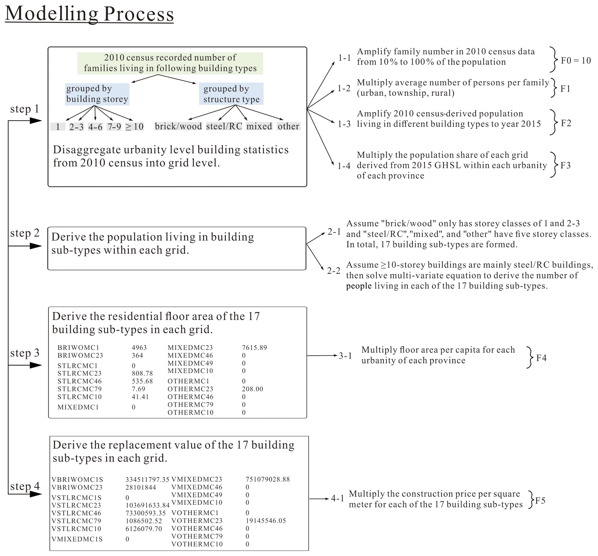
Figure 3Flowchart of the residential building stock modelling process adopted in this paper (see context in Sect. 2.4 for more details).
2.4.1 Step 1 – disaggregate urbanity-level building-related statistics from the 2010 census into grid level
Like in many other countries, the population and housing census data in mainland China are particularly surveyed for residential buildings. Therefore, the building stock model developed in this paper is for residential building stock. As listed in Table 2, building-related statistics extracted from the 2010 census records include the number of families living in buildings grouped either by the number of storeys (i.e. 1, 2–3, 4–6, 7–9, ≥10) or by structure type (i.e. steel and reinforced concrete, mixed, brick and wood, other; hereafter “steel and reinforced concrete” is abbreviated as steel and RC, and “mixed” refers to different combinations of masonry buildings), the average population per family, and the average floor area per capita. For each urbanity level of each province, the number of families living in buildings grouped by storey number or structure type is extracted from the long table of the 2010 census, which is based on the survey of only 10 % of the total population in mainland China (as noted in Table 1). Therefore, the number of families living in different building types needs to be extended from 10 % to 100 % of the population first. This is achieved directly by multiplying the number of families by the factor of 10 (namely factor F0 in Step 1-1 of Fig. 3). Multiplying the number of families with the average number of people per family (namely factor F1 in Step 1-2 of Fig. 3, with values listed in Table 2) provides the number of people living in buildings grouped by storey number (1, 2–3, 4–6, 7–9, ≥10) or structure type (steel and RC, mixed, other, brick and wood) for each urbanity of each province.
The geo-coded population grids in the 2015 GHSL profile with assigned urbanity attributes (Sect. 2.3) and the number of people living in buildings grouped by storey number or structure type derived for each urbanity of each province seem to allow the direct disaggregation of the 2010 census statistics into the 2015 GHSL grids. However, the GHSL population is for the year 2015, while the derived population living in different structure type or storey class from the building-related statistics is for the year 2010. The increase in population and buildings from 2010 to 2015 must be considered. Here we assume that the increase in population living in buildings grouped by storey class or structure type from 2010 to 2015 is equal to the increase in population from the 2010 census records to the 2015 GHSL profile. Therefore, for each urbanity of each province, the derived number of people living in building types grouped by storey class or structure type (after performing Step 1-1 and 1-2 in Fig. 3) will be further amplified to the year 2015 by multiplying by the population amplification factor (namely factor F2 in Step 1-3 of Fig. 3). For each urbanity of each province, the value of F2 is equal to the ratio of the 2015 GHSL population to the sum of the population living in buildings of different occupancy types. For example, in urbanity “1001” of Anhui Province in Table 2, the value of F2 (1.32) results from the ratio of the 2015 GHSL population (12 165 295) to the product of the number of families living in three occupancy types (; based on surveys of 10 % of the whole population), the average number of people per family (F1 =2.71), and the factor to extend the survey of 10 % of the population to 100 % of the population (F0 = 10), namely .
Thus, for each urbanity of each province, the number of people living in buildings grouped by storey class or structure type in 2015 is derived by multiplying the original number of families living in different building types (based on surveys of 10 % of the whole population) in Table 2 by the factors F0, F1, and F2. These urbanity-level statistics can be disaggregated into the geo-coded grids of the 2015 GHSL profile. The population share in each grid (relative to the sum of population of grids with the same urbanity) is used as the disaggregation weight (namely factor F3 in Step 1-4 of Fig. 3). By multiplying the urbanity-level population living in buildings grouped by storey class or structure type with the disaggregation factor F3 of each grid, the grid-level number of people living in buildings grouped by storey class or structure type can be directly derived.
2.4.2 Step 2 – derive the population living in the 17 building subtypes within each grid
As explained in Sect. 2.4.1, after multiplying the original number of families living in different building types extracted from the 2010 census records (Table 2, based on surveys of 10 % of the whole population) by the factors F0, F1, F2, and F3 in Step 1 of Fig. 3, the grid-level populations living in buildings grouped either by the number of storeys (1, 2–3, 4–6, 7–9, ≥10) or by structure type (steel and RC, mixed, other, brick and wood) are derived for all geo-coded grids in the 2015 year level. To further estimate the residential building floor area and replacement value in each grid, we need to evaluate the unit construction prices of the building types in each grid. Currently, the building types are grouped either by storey number or by structure type, and they need to be reclassified into building subtypes with both storey class and structure type attributes. Then it will be easier and more reasonable to estimate the unit construction prices of these building subtypes compared to the estimation made in studies based on building occupancy type (e.g. Wu et al., 2019).
In the following description, we first introduce the reclassification of building subtypes with both storey class and structure type attributes. Then we estimate the population living in each of the 17 building subtypes. Based on the statistics of average floor area per capita in each urbanity level extracted from the 2010 census records (as listed in Table 2), the total floor area of each of the 17 building subtypes in each grid can be derived. Finally, for each building subtype, their replacement value emerges from a multiplication of the floor area with the unit construction price.
By combining the five storey classes (1, 2–3, 4–6, 7–9, ≥10) with the four structure types (steel and RC, mixed, other, brick and wood), the building types in the 2010 census records can be initially reclassified into 20 building subtypes. According to Hu et al. (2015) and Wang et al. (2018), most brick and wood buildings are with quite low height (1, 2–3), while steel and RC buildings are generally quite high, with 10-storey height and above. Therefore, in this paper it is assumed that for the “brick and wood” structure type, there are only two storey classes (1, 2–3), while for “steel and RC”, “mixed”, and “other” structure types, all five storey classes (1, 2–3, 4–6, 7–9, ≥10) are available (namely the assumptions in Step 2-1 and 2-2 of Fig. 3). Thus, the number of building subtypes with known storey class and structure type is reduced from 20 to 17. The abbreviations of these 17 building subtypes are listed in Table 4.
Table 4Average unit construction price (per m2) for each of the 17 building subtypes used in this paper.

After performing the calculations in Step 1 of Fig. 3, the grid-level populations living in buildings grouped either by the number of storeys (1, 2–3, 4–6, 7–9, ≥10) or by structure type (steel and RC, mixed, other, brick and wood) are derived for all geo-coded grids. Thus, we know in each grid the number of people living in buildings of the five storey classes, but we do not know for each storey class how the population is distributed among the four structure types. Also, we know how many people live in steel and RC buildings or other structure types, but for each structure type, we do not know how they are distributed into the five storey classes. For each grid, to derive the number of people living in each of the 17 building subtypes with known structure type and storey class, we need to solve 17 unknown variables from 9 equations. The 9 equations are listed as follows:
The 17 to-be-solved variables on the left side of this equation set represent the numbers of populations living in the 17 buildings subtypes (as defined in Table 4); on the right side, the numbers indicate the number of people living in buildings classified by five storey classes and four structure types, which are already known after performing the calculations in Step 1 of Fig. 3. Since this set of 9 equations contains 17 unknown variables, it is an underdetermined linear problem. In order to provide values for the 17 unknowns, additional assumptions have to be utilized.
The strategy we employ here to derive the population living in each of the 17 building subtypes of each grid in a series of distribution steps based on a prioritized ranking of building types and storey classes. For example, we first assign storey class 1 buildings to the brick–wood structure type and distribute the storey class ≥10 as the steel–RC structure type (following the assumptions in Step 2-1 and 2-2 of Fig. 3). Although this distribution strategy may deviate from the actual situation, the basic requirement that in each grid the sum of the population living in the 17 building subtypes is equal to the population living in building types grouped by structure type or by storey class is satisfied. The main distribution steps are summarized in Appendix A.
2.4.3 Step 3 – derive the residential floor area of the 17 residential building subtypes in each grid
Based on the distribution processes in Appendix A, we derive the number of people living in each of the 17 building subtypes in each grid. To derive the residential floor area of each building subtype, the average residential floor area per capita is needed, which is given in the short table of 2010 census (namely factor F4 in Step 3-1 of Fig. 3) for each urbanity level of each province. Therefore, the floor area of the 17 building subtypes in each grid can be directly derived. This grid-level residential building floor area distribution map is available from the Supplement online. Comparison between the modelled floor area and the 2010 census-recorded floor area for residential buildings at the county or district level is performed in Sect. 3.2.2.
2.4.4 Step 4 – derive the replacement value of the 17 residential building subtypes in each grid
With the residential building floor area for each building subtype in each grid being derived in Step 3, to get the corresponding replacement value, the unit construction prices of the 17 building subtypes need to be estimated (namely factor F5 in Step 4-1 of Fig. 3). Given the uniqueness of the building reclassification strategy adopted in this paper, there are no standard unit construction price evaluations for the building subtypes we use here. Therefore, we estimate the unit construction prices of the 17 building subtypes (as listed in Table 4) by averaging the construction prices given in different literature (e.g. 2015 China Construction Statistical Yearbook, the World Housing Encyclopedia, real-estate agency reports, etc.). For the 17 building subtypes in each grid, by multiplying their floor area by the corresponding unit construction price in Table 4, their replacement values can be directly derived. This grid-level residential building replacement value distribution map is also available from the Supplement online. We emphasize that in this paper, the term “replacement value” refers to the amount of money needed to rebuild a property exactly as it is before its destruction regardless of any depreciation, namely the gross capital stock. A prefecture-level comparison between our modelled residential building replacement value and the wealth capital stock value in Wu et al. (2014) is given in Sect. 3.2.1.
3.1 Results
3.1.1 Modelled floor area and replacement value for residential buildings in each urbanity of each province
The grid-level residential building floor area and replacement value (unit: CNY, in 2015 prices) are aggregated into urbanity level (urban, township, rural) for each province, as listed in Table 5. The total modelled residential building floor area for mainland China in 2015 reaches 42.31 billion m2. By applying the same unit construction prices for the same 17 building subtypes in all the urban, township, and rural areas of the 31 provinces, the initially modelled replacement value of residential buildings in mainland China is CNY 77.8 trillion (in 2015 prices). It is clear that like all other building stocks, the Chinese building stock is a complicated economic, physical, and social system (Yang and Kohler, 2008). There are significant differences across the country in terms of economic development level, geographic and climatic diversity, and standardization in building construction. Therefore, it is mainly for computational convenience that this paper applies the same unit construction price for all the provinces and all the urbanity levels. To improve accuracy in future seismic risk assessment, the unit construction prices of specific building types in the target study area should be adjusted accordingly.
Table 5The modelled floor area and replacement value of residential buildings in the urban, township, and rural urbanities of the 31 provinces in mainland China.

Note: (a) in this paper, for each of the 17 building subtypes in each grid, the same unit construction price is used to derive the replacement value in different urbanities and provinces, and (b) the modelled floor area and replacement value are for residential buildings (see context in Sect. 3.1.1 for more details).
3.1.2 An example illustrating the distribution of modelled floor area in Shanghai
For better visualization of the modelled floor area at grid level and to help potential readers to conduct direct comparison with other reports or modelling results, we plot the residential building floor area distribution map and the 2015 GHSL population of Shanghai as an example. As can be seen from Fig. 4, grids with a high density of floor area typically cluster in the downtown area (including eight administrative districts, namely Yangpu, Hongkou, Zhabei, Putuo, Changning, Xuhui, Jing'an, and Huangpu) and the Pudong District. This corresponds to the fact that these districts are the most developed in Shanghai.
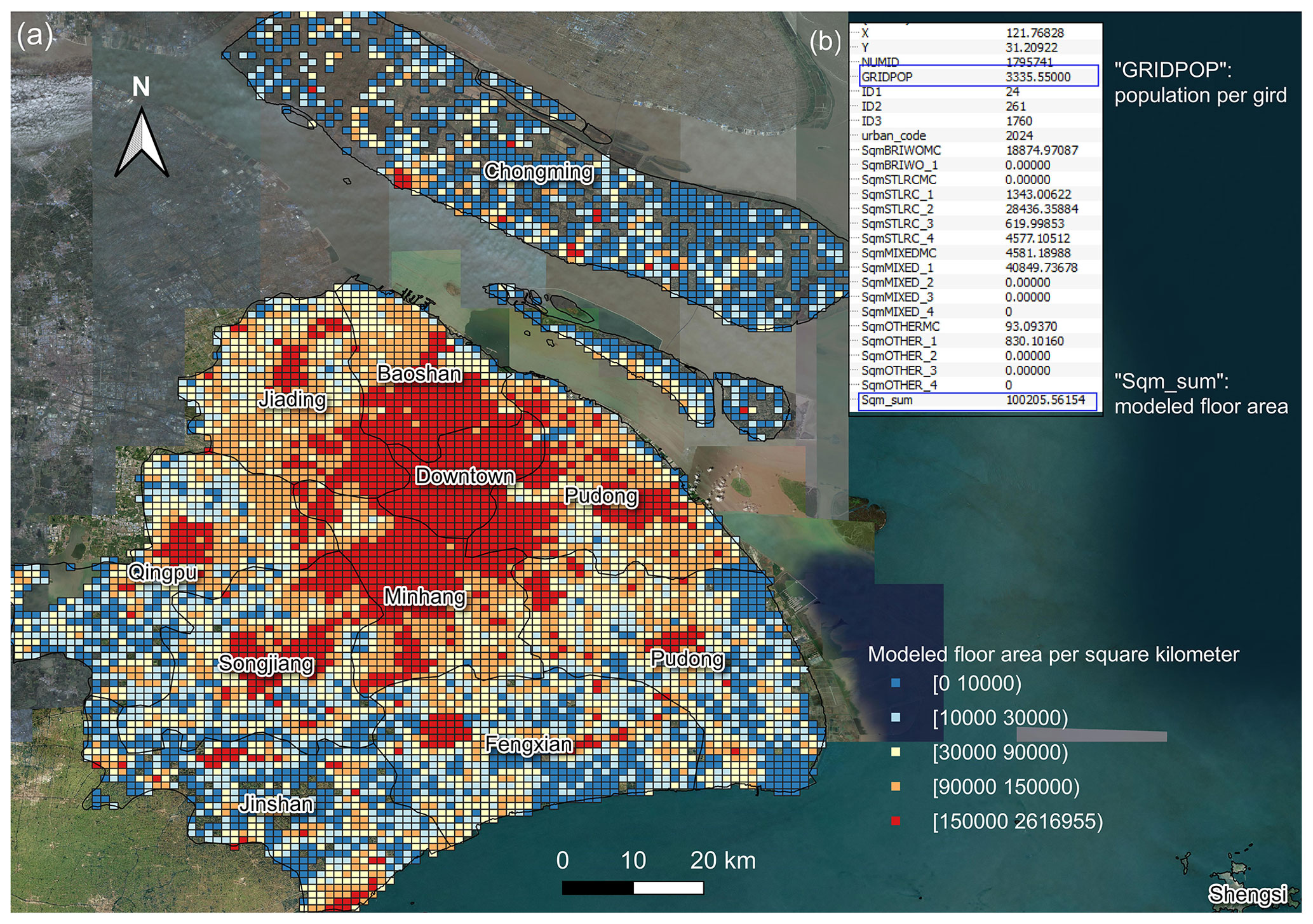
Figure 4An example illustrating the building stock model of Shanghai: (a) the distribution of modelled floor area (unit: m2) in each 1 km × 1 km grid (note that the legend in Fig. 4 is different from that in Fig. 2) and (b) a table showing the modelled floor area of the 17 building subtypes, the total population “GRIDPOP”, and the total modelled floor area “Sqm_sum” in an example grid. This figure is plotted by using the QGIS platform, and the background satellite map is provided by the Bing map service (© Microsoft).
3.2 Performance evaluation
As of now, we have developed a high-resolution (1 km × 1 km) residential building stock model (in terms of floor area and replacement value) for mainland China. This model is established by disaggregating the urbanity-level building-related statistics in 2010 census records into grid level and using the 2015 GHSL geo-coded population as the disaggregation weight. Due to the approximations and assumptions made in the modelling process, the reasonability and consistency of the modelled results need to be evaluated. Due to the typical lack of official statistics on high-resolution building stock from the government (Wu et al., 2018), direct comparison of the modelled floor area and replacement value at grid level with that from official census or statistical yearbooks is not instantly available. Instead, we compare our modelled results with other studies or census records at a coarser level. Moreover, since the development of such a high-resolution residential building model is mainly targeted for seismic risk assessment in mainland China, we also apply our modelled results to seismic loss estimation combining with the 2008 Wenchuan Ms 8.0 earthquake intensity map and an empirical loss function. The estimated losses are compared with those recorded in affected counties and districts of Sichuan Province.
3.2.1 Prefecture-level comparison between the modelled residential building replacement value and the net capital stock value estimated in Wu et al. (2014)
Due to the lack of officially published datasets on the value of fixed capital stock in China (Wu et al., 2018), previous studies (e.g. Holz, 2006; Wang and Szirmai, 2012) mainly employed the perpetual inventory method (PIM), in which economic indicators (e.g. gross fixed capital formation, total investment in fixed assets, etc.) are used. The resolutions of these estimations were almost exclusively limited at the national or provincial level (Wu et al., 2014). This coarse spatial resolution forms a major obstacle in applying the model in disaster loss estimation, where high-resolution hazard data are used. To overcome this gap, Wu et al. (2014) estimated the net capital stock values from 1978 to 2012 for 344 prefectures in mainland China by using the PIM. In their Appendix Table A1, the net capital stock values calculated in 2012 prices for 344 prefectures were provided, with the depreciation of all exposed assets (i.e. residential and non-residential building structures, tools, machinery, equipment, and infrastructure) being considered.
To compare with the net capital stock value in Wu et al. (2014), the grid-level residential building replacement value modelled in this paper (namely the gross value of residential building stock) was aggregated into the prefecture level. Pearson's correlation coefficient (R2) was used to measure the degree of collinearity between two datasets, with higher R2 indicating a stronger correlation. As shown in Fig. 5, there is a high correlation (R2=0.9512) between our residential building replacement values and the net capital stock values in Wu et al. (2014) at the prefecture level. The absolute replacement value of residential buildings is around 0.54 times the net capital stock value in Wu et al. (2014). To explain this discrepancy, we collected the annual fixed asset investment on residential buildings and on all types of buildings for each of the 31 provinces during the years 2004–2014 from the statistical yearbooks (detailed statistics are available from the Supplement online). As can be seen from Fig. 6, for each province the sum of fixed asset investment on residential buildings during 2004–2014 is around 0.45 times the investment on all types of buildings, quite close to the 0.54 ratio in Fig. 5. The replacement value we estimate is purely for residential buildings without depreciation, while the net capital stock value in Wu et al. (2014) includes depreciation of all exposed assets (residential, non-residential buildings, infrastructures, and equipment). Thus, we consider our model results to be reasonable.
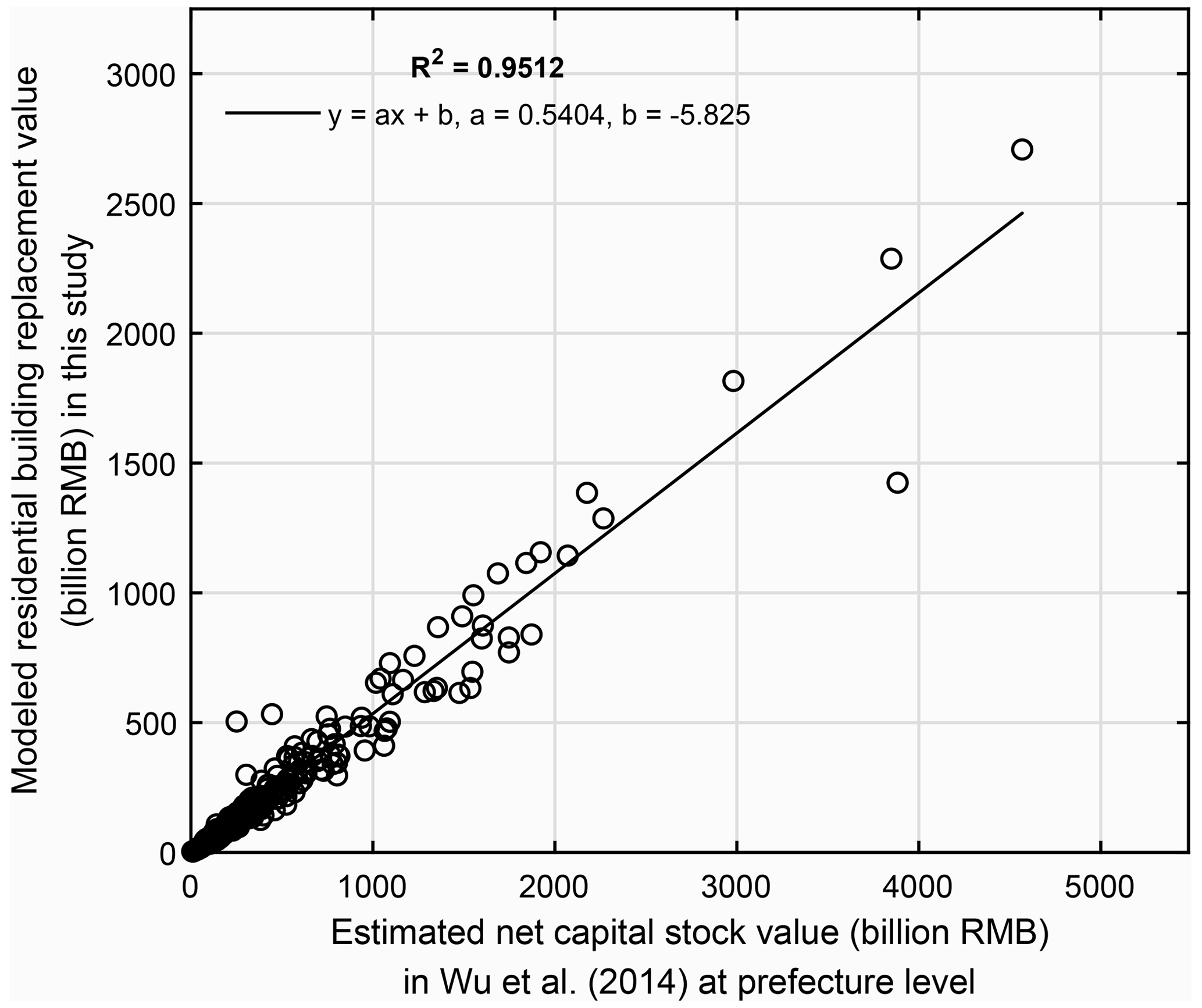
Figure 5Prefecture-level comparison of the modelled residential building replacement value in this paper (unit: billions of CNY in 2015 prices) with the net capital stock value estimated in Wu et al. (2014) by using the perpetual inventory method (unit: billions of CNY in 2012 prices). Note: the net capital stock value estimated in Wu et al. (2014) includes the depreciated value of all exposed elements, namely the residential buildings, non-residential buildings, infrastructures, and equipment (see context in Sect. 3.2.1 for more details).
3.2.2 County- and prefecture-level comparison between modelled residential building floor area and records in the 2010 census
Compared with previous studies related to building stock modelling in China, we have used finer urbanity-level building-related statistics as input to generate the grid-level residential building stock model. In each urbanity, the building-related statistics extracted from the 2010 census records are from areas with a similar development background, but they belong to different administrative units (i.e. prefectures and counties). Also, within the same prefecture or county, the geo-coded grids are of different urbanity attributes. Therefore, the reliability of our model can be better proved if the modelled results correlate well with actual records at the county or prefecture level. After a thorough search, we find that county-level records of residential building floor area are also available for 28 provinces in mainland China, except for Hunan, Liaoning, and Sichuan provinces, for which only prefecture-level records of residential building floor area can be found from the 2010 census records. Then, to compare our modelled floor area with the 2010 census records at the county or prefecture level, the modelled grid-level residential building floor area was first aggregated into counties or districts for the 28 provinces as well as prefectures for Hunan, Liaoning, and Sichuan, respectively. The final comparison between our estimated residential building floor area with that recorded in the 2010 census is plotted in Fig. 7.
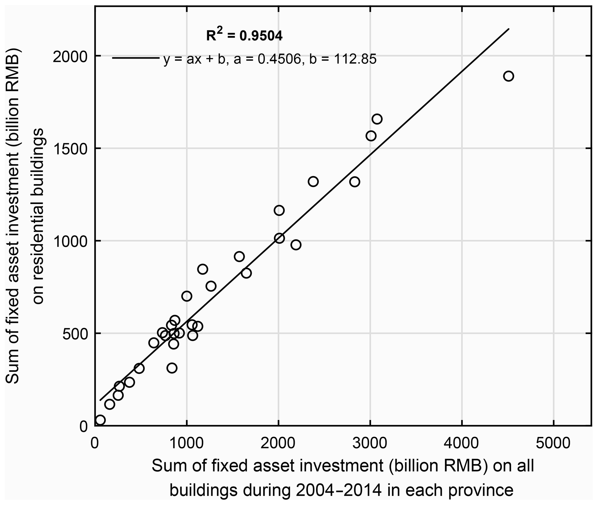
Figure 6Comparison of the sum of the annual fixed asset investment (unit: billions of CNY) on residential buildings with investment on all types of buildings during 2004–2014 in each of the 31 provinces in mainland China. Detailed investment statistics are available from the Supplement.
As can be seen from Fig. 7, there is a high correlation (R2=0.9376) between modelled floor area and that recorded in the 2010 census at the county or prefecture level. The regression relation indicates that our modelled floor area for 2015 is around 1.14 times that in the 2010 census. In Step 1-3 of the modelling process (Fig. 3), for each urbanity level of each province, the building-related statistics extracted from the 2010 census records were amplified to the 2015 level by multiplying by the factor F2. Mathematically speaking, F2 is the ratio of the 2015 GHSL population to the 2010 census-recorded population. F2 is 1.13 for the whole of mainland China, which can be derived by following the derivation process of F2 illustrated in Sect. 2.4.1 based on the statistics in Table 2. Therefore, we consider the ratio of 1.14 between our modelled floor area for 2015 and that recorded in the 2010 census at the county or prefecture level to be quite reasonable. For each province, we also plotted the correlation analyses for the population (between the 2015 GHSL population and 2010 census-recorded population) and for the residential building floor area (between the modelled floor area and the 2010 census-recorded floor area), which are available from the Supplement online. The corresponding regression parameters and correlation coefficients for the population and the residential building floor area of each province are listed in Table 6.
Table 6The regression parameters and correlation coefficients for population and floor area in each province.
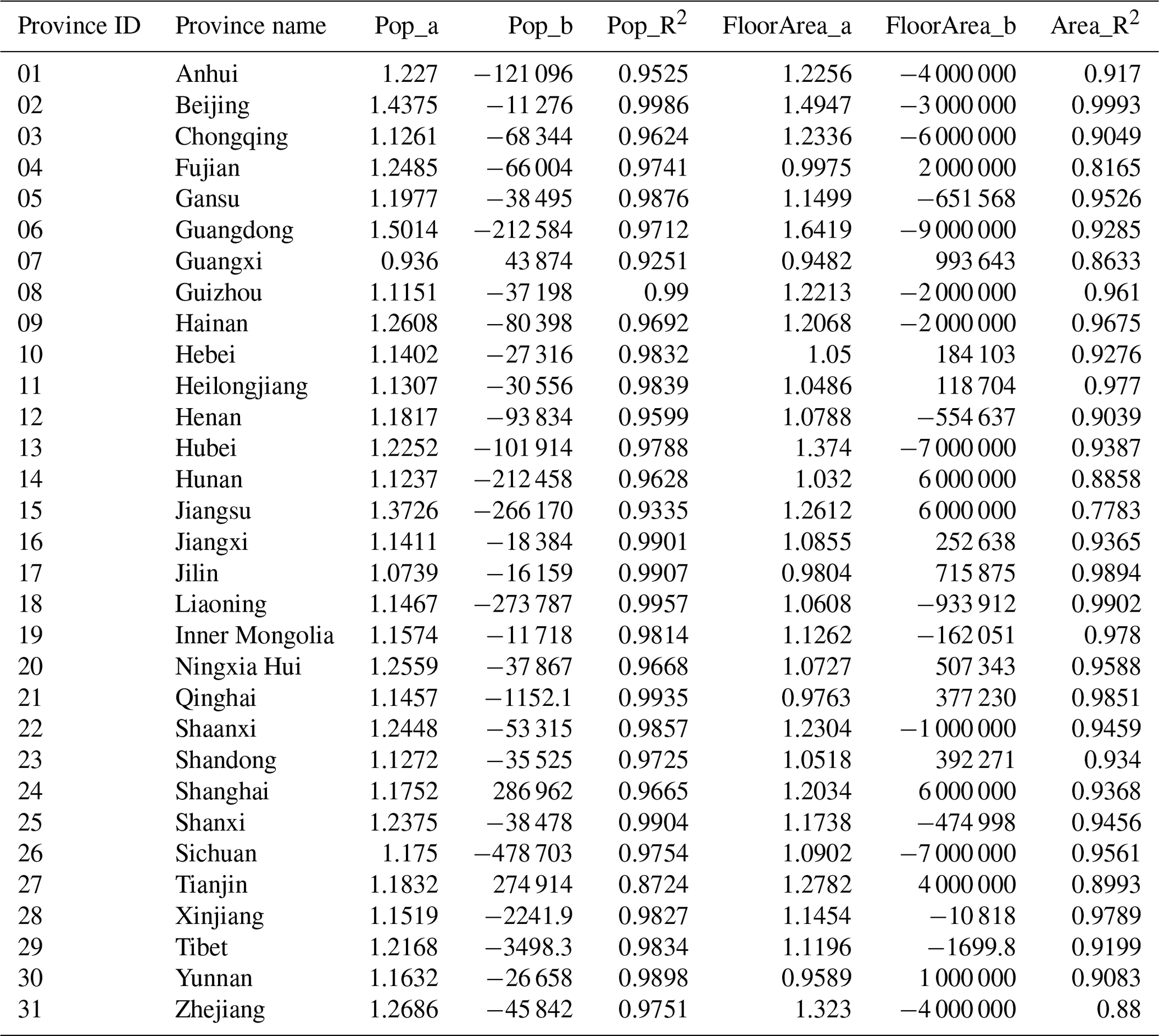
Note: “Pop_a” and “Pop_b” are the linear regression parameters between the 2015 GHSL population and the 2010 census-recorded population; “FloorArea_a” and “FloorArea_b” are the linear regression parameters between the modelled residential building floor area in this paper and that extracted from the 2010 census records; “Pop_R2” and “FloorArea_R2” are the correlation coefficients of population and floor area, respectively. For Hunan, Liaoning, and Sichuan provinces, the population and floor area comparisons are compared at the prefecture level, while for the other 28 provinces, the population and floor area comparisons are at the county level. The correlation analysis figures for each of the 31 provinces are available from the Supplement online (see the context in Sect. 3.2.2 for more details).
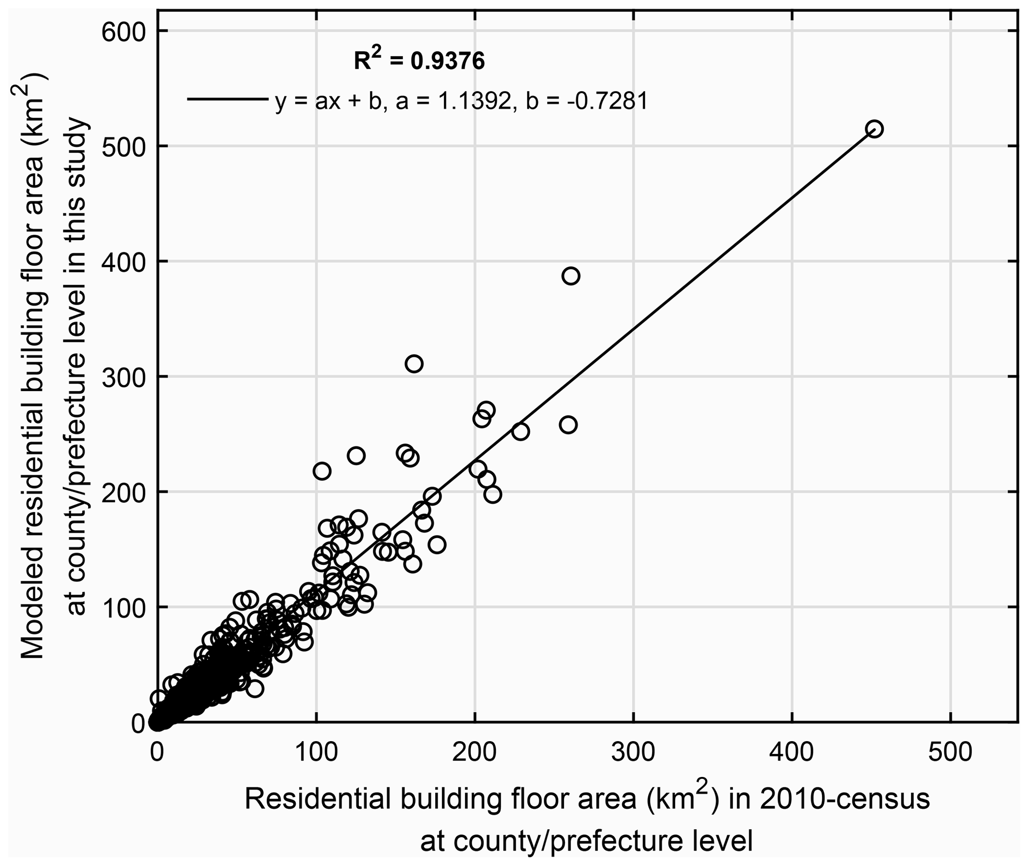
Figure 7County- and prefecture-level comparison of the modelled residential building floor area (km2) in this paper with that recorded in the 2010 census for 31 provinces in mainland China (see context in Sect. 3.2.2 for more details).
From Table 6 we can see that the correlation between the 2015 GHSL population and the 2010 census-recorded population and the correlation between the modelled floor area and the 2010 census-recorded floor area are generally very high for a majority of provinces (with R2≥0.9). This indicates the plausibility of choosing the 2015 GHSL population as the ancillary information to disaggregate the urbanity-level building-related statistics and the reliability of our modelled floor area at the county or prefecture level. However, it is also worth noting that for coastal provinces like Fujian and Jiangsu, the correlation coefficients of floor area are lower (with R2<0.82). We explain this discrepancy by an overpredicted population in the 2015 GHSL profile for the capital or the most developed cities in these provinces (as can be checked from the population correlation analyses for these provinces from the Supplement online). Many people tend to work in the capital or the most developed cities without being officially registered as residents. These people are not counted in the 2010 census of these cities but are included in the 2015 GHSL population density profile, which is derived from remote sensing data combined with the actual population density.
3.2.3 Application of the residential building stock model to seismic loss estimation
Since the residential building model developed in this paper is targeted for seismic risk analysis, we now use the modelled replacement value to estimate the seismic loss to residential buildings in Sichuan Province caused by the Wenchuan Ms 8.0 earthquake. The hazard component used for this loss estimation is the macro-seismic intensity map of the 2008 Wenchuan Ms 8.0 earthquake (Fig. 8), which was issued by the China Earthquake Administration (CEA) based on post-earthquake field investigations. The vulnerability function used was the empirical loss function developed in Daniell (2014, p. 242) for mainland China, which provides the relation between macro-seismic intensity and loss ratio (the ratio between repair cost and replacement cost of buildings damaged in an earthquake). This empirical vulnerability function was developed based on reported seismic damage and loss related to earthquakes that occurred in mainland China in the past few decades. Such information was retrieved through an extensive collection of damage and loss records from journals, books, reports, conference proceedings, and even newspapers.
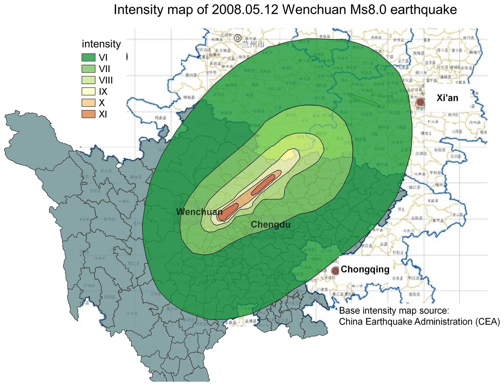
Figure 8Macro-seismic intensity map of the 2008 Wenchuan Ms 8.0 earthquake, modified after the base intensity map issued by the China Earthquake Administration (CEA).
Our estimated seismic loss of residential buildings in Sichuan Province due to the Wenchuan Ms 8.0 earthquake is around CNY 432 billion (in 2015 prices). The spatial distribution of loss ratios, i.e. the ratio of the estimated loss to the total residential building replacement value in counties and districts of Sichuan Province, is shown in Fig. 9. In other reports and studies on the loss assessment of the Wenchuan earthquake, e.g. in Yuan (2008), the estimated loss to residential buildings in Sichuan Province was around CNY 170 billion (in 2008 prices). The officially issued loss estimated by the Expert Panel of Earthquake Resistance and Disaster Relief (EPERDR, 2008) to residential buildings in Sichuan Province was around CNY 98.3–435.4 billion, with the median loss around CNY 212.32–247.25 billion (in 2008 prices). It should be noted that in these studies, the unit construction price used for rural, urban, and township building replacement was around CNY 800–1500/m2, which is – of the unit construction price used in this paper as listed in Table 4. Dividing our estimated loss by the factor of 1.5–2.5, the difference in construction price used in this paper and previous studies is eliminated, and the estimated loss based on our building exposure model goes from CNY 432 billion to around CNY 144–288 billion (in 2015 prices), which is now consistent with that estimated by EPERDR and Yuan (2008). This simple test further indicates the applicability of our model in seismic loss estimation. Thus, the grid-level residential building floor area and replacement value developed in this paper can be regarded as reliable exposure inputs for future seismic risk assessment in mainland China.

Figure 9Distribution of seismic loss ratio (the ratio between repair cost and replacement cost) of residential buildings in affected districts and counties of Sichuan Province due to the 2008 Wenchuan Ms 8.0 earthquake. Black contours represent the extent of each intensity zone of the Wenchuan earthquake (see context in Sect. 3.2.3 for more details).
According to studies on assessing the resolution of exposure data required for different types of natural hazards (e.g. Chen et al., 2004; Thieken et al., 2006; Bal et al., 2010; Figueiredo and Martina, 2016; Röthlisberger et al., 2018; Dabbeek et al., 2021), the 1 km × 1 km residential building stock model developed in this paper is sufficient for seismic risk assessment. However, limitations in our model are inevitable due to the assumptions and approximations employed in the modelling process. For example, when disaggregating the urbanity-level building-related statistics in the 2010 census into grid level and scaling these statistics from 2010 to 2015, we assume that the number of residential buildings in each grid is proportional to its population weight, and the increase in building-related statistics of each urbanity is equal to its population increase, which needs to be carefully evaluated by the local development of building stock (e.g. Fuchs et al., 2015). Secondly, to derive the population living in each of the 17 building subtypes in each grid, we assume that brick and wood buildings are limited to storey classes 1 and 2–3 and distribute the number of steel and RC buildings to storey class ≥10 first, which may not be fully consistent with the real cases. Furthermore, we use the same unit construction prices for the same building subtypes regardless of their variation across province and urbanity, which also needs certain readjustment when applying our modelled residential building replacement value into actual seismic risk analyses.
In the future, with the increasing availability of open-source datasets that track individual building features in detail, the current limitations in this paper can possibly be overcome. Attempts have been made to combine publicly available building vector data (which contain the spatial location, footprint, and height of each building) and census records to improve the exposure estimation (e.g. Figueiredo and Martina, 2016; Wu et al., 2019; Paprotny et al., 2020). Algorithms to extract building footprints and height from aerial imagery and using computer vision techniques have been used by commercial companies like Google and Microsoft (Parikh, 2012; Bing Maps Team, 2014). More recently, by using an unmanned aerial vehicle and a convolutional neural network, Xiong et al. (2020) introduced an automated building seismic damage assessment method in which not only the 3D building structure can be constructed, but also the building damage state can be predicted automatically with an accuracy of 89 %. In addition, Li et al. (2020) developed the first continental-scale dataset on 3D building structure (including building footprint, height, and volume) at 1 km × 1 km resolution for Europe, China, and the US by using random forest models fed with remote sensing and synthetic aperture radar imagery data. Liu et al. (2021) developed the urban floor area map for mainland China at 130 m × 130 m resolution based on high-spatial-resolution nighttime light LUOJIA 1-01 images, a population map, and a single building dataset encompassing 71 cities. Ji et al. (2020) generated the 10 m × 10 m resolution model of rural settlements in the Yangtze River Delta of China by using the multi-source remote sensing datasets with the Google Earth Engine platform. Cao and Huang (2021) proposed a multi-spectral, multi-view, and multi-task deep network (called M3Net) for building height estimation. They estimated the building height at a spatial resolution of 2.5 m × 2.5 m for 42 Chinese cities. Comparison with the results in Li et al. (2020) indicated that the M3Net method in Cao and Huang (2021) can better alleviate the saturation effect of high-rise building height estimation than the random forest method used in Li et al. (2020). We take these attempts as an indicator that the high-resolution modelling of building stock for individual buildings will become more widely available in the future.
In this paper, a 1 km × 1 km resolution residential building stock model (in terms of floor area and replacement value) targeted for seismic risk analysis for mainland China is developed by using the 2015 GHSL population density profile as the bridge and by disaggregating the finer urbanity-level 2010 census records into grid level for each province. In each grid, a building distribution strategy is adopted to derive the number of people living in each of the 17 building subtypes with structure type and storey class attributes, based on which the floor area and replacement value of each building subtype are derived. In each urbanity of each province, the building-related statistics extracted from the 2010 census records are from areas with a similar development background but different administrative units (i.e. prefectures and counties). Therefore, to evaluate the model performance, the residential building replacement value is first compared with the net capital stock value estimated in Wu et al. (2014) at the prefecture level. These two datasets are well correlated, and the former is around 0.45 of the latter, which is quite reasonable referring to the fact that for each province the sum of fixed asset investment value on residential buildings is around 0.54 of the sum of investment values on all types of buildings during 2004–2014. Furthermore, county- and prefecture-level comparisons of the residential floor area modelled in this paper with records from the 2010 census are also conducted. It turns out that the modelled and recorded residential building floor areas are highly compatible for many counties and prefectures. To further check the applicability of the modelled results in seismic risk assessment, an empirical seismic loss estimation is performed based on the intensity map of the 2008 Wenchuan Ms 8.0 earthquake, the empirical loss function in Daniell (2014), and our modelled replacement value of residential buildings in Sichuan Province. By reducing the difference in unit construction price used in this paper and other studies, our estimated loss range is consistent with the loss derived from damage reports based on field investigation. These comparisons indicate the reliability of the geo-coded grid-level residential building exposure model developed in this paper. More importantly, the whole modelling process is fully reproducible, and all the modelled results are available from the Supplement online, which can also be easily updated when more recent or detailed census data are available.
In Appendix A, to derive the population living in each of the 17 building subtypes of each grid, the distribution strategy mentioned in Sect. 2.4.2 is explained in detail. In addition, a MATLAB script is provided to help understand this strategy.
For each grid, to derive the population living in each of the 17 building subtypes (their abbreviations are given in Table 4), namely the 17 to-be-solved variables on the left side of the equation set in Sect. 2.4.2, a series of distribution steps based on a prioritized ranking of building types and storey classes are used in this paper. A MATLAB script and an input file illustrating the distribution processes are also available from the Supplement online. With the help of the MATLAB script, it will be easier to understand the distribution steps as follows.
-
For the brick–wood structure type, in each grid if NumBRIWO<Numstorey1, the population living in the brick–wood structure type (NumBRIWO) is first placed into storey class 1, then we get BRIWOMC1= NumBRIWO, and the remaining population living in the brick–wood structure type is 0, while the remaining population living in storey class 1 is (Numstorey1−NumBRIWO). But if NumBRIWO≥Numstorey1, then the population living in storey class 1 buildings (Numstorey1) is assumed to be in the brick–wood structure type, and we get BRIWOMC1=Numstorey1, and the remaining population living in brick and wood buildings is (NumBRIWO−Numstorey1), while the remaining population living in storey class 1 is 0.
-
If the remaining population living in brick and wood buildings , then they are placed into storey class 2–3 class, and we get or , and the remaining population in storey class 2–3 is . But if , we directly assign BRIWOMC23=Numstorey23, and the remaining population living in brick and wood buildings is .
-
For steel–RC structure type, in each grid if , the population living in the steel–RC structure type (NumSTLRC) is first placed in the storey class ≥10, and we get STLRCMC10=NumSTLRC. Then the remaining population living in the storey class ≥10 is , while the remaining population living in the steel–RC structure type is 0. But if , then we directly assign , and the remaining population living in the steel–RC structure type is , while the remaining population living in the storey class ≥10 is 0.
-
Following the above step (3), if , the remaining population living in the steel–RC structure type is compared with the population living in other storey classes and distributed into the remaining storey classes from the highest to the lowest, assuming that the smallest population in steel and RC would be in storey class 1. Then we get , STLRCMC79=Numstorey79, or STLRCMC79=0; , or STLRCMC46=Numstorey46, or STLRCMC46=0; , or , or STLRCMC23=0; , or , or STLRCMC1=0.
-
After determining the population living in seven building subtypes (BRIWOMC1, BRIWOMC23, STLRCMC10, STLRCMC79, STLRCMC46, STLRCMC23, STLRCMC1) and the remaining population living in each of the five storey classes, to derive the population living in storey class with structure type “mixed” and “other”, we assume that the populations living in the five storey classes of the “mixed” structure type are equal to the product of the remaining population in each storey class and the ratio of . Similarly, the populations living in the five storey classes of the “other” structure type are equal to the product of the remaining population in each storey class and the ratio of .
The access to data used or mentioned in this paper is as follows: (1) 2010 China Sixth Population Census tabulation (http://www.stats.gov.cn/tjsj/pcsj/rkpc/6rp/indexch.htm, Population Census Office of the State Council, and Department of Population and Employment, Bureau of Statistics, 2021); (2) 2015 Global Human Settlement Layer (GHSL) population density profile (https://ghsl.jrc.ec.europa.eu/datasets.php#inline-nav-ghs_pop2019, European Commission, Joint Research Centre, 2021); (3) the spatial administrative boundaries from the National Geomatics Centre of China (http://www.ngcc.cn/ngcc/html/1/391/392/16114.html, Resource and Environment Science and Data Center, 2021); (4) the Globcover land cover maps (http://due.esrin.esa.int/page_globcover.php, European Space Agency, 2021); (5) the GLC2000 land cover classes (https://forobs.jrc.ec.europa.eu/products/glc2000/legend.php, European Commission, 2021b); (6) the MODIS imaging project (https://modis.gsfc.nasa.gov/about/, National Aeronautics and Space Administration, 2021a); (7) the GlobeLand30 project (http://www.globallandcover.com/, Ministry of Natural Resources, 2021); (8) the DMSP-OLS nighttime light datasets (https://data.noaa.gov/metaview/page?xml=NOAA/NESDIS/NGDC/STP/DMSP/iso/xml/G01119.xml&view=getDataView&header=none, National Centres for Environmental Information, 2021); (9) OpenStreetMap (https://www.openstreetmap.org/, OpenStreetMap Foundation, 2021); (10) Gridded Population of the World (GPW; http://sedac.ciesin.columbia.edu/gpw/global.jsp, National Aeronautics and Space Administration, 2021b); (11) Global Rural-Urban Mapping Project population (GRUMP population; https://sedac.ciesin.columbia.edu/data/collection/grump-v1, National Aeronautics and Space Administration, 2021c); (12) LandScan global population datasets (https://landscan.ornl.gov/landscan-datasets, Oak Ridge National Laboratory, 2021); (13) WorldPop/AsianPop (https://www.worldpop.org/geodata/listing?id=29, University of Southampton, 2021); (14) PopGrid China (http://www.geodata.cn/thematicView/datadetails.html?dataguid=161949057751763&pdate=2014E5B9B408E69C88&t=181742444058870, National Earth System Science Data Centre, 2021); (15) an example illustrating the multivariate equation-solving process in Sect. 2.4.2, including the input file and the MATLAB script that are available from the online supplement (available at https://doi.org/10.5281/zenodo.4669800, Xin et al., 2021).
DX conducted the data collection and preparation, analyses of results, and model validation and prepared the draft manuscript. JED guided the data collection and preparation process, developed the modelling methodology, and performed the calculation of and co-analysed the results. HHT and FW supervised the project and provided advice and feedback in the process. All authors contributed to the revision of the manuscript.
The authors declare that they have no conflict of interest.
Publisher's note: Copernicus Publications remains neutral with regard to jurisdictional claims in published maps and institutional affiliations.
The authors thank the editor Sven Fuchs for actively monitoring the whole review process. We also appreciate the efforts and time spent by the two anonymous reviewers for this work and the two reviewers from a previous round of submission. Their suggestions have greatly improved the quality of this work. We also want to thank the careful review of the language copy-editor and the typesetter of the journal NHESS. Their hard work has greatly improved the presenting quality of this work.
This research was jointly supported by the China Scholarship Council (CSC),
the Karlsruhe House of Young Scientists (KHYS) from the Karlsruhe Institute
of Technology (KIT), the China Postdoctoral Science Foundation (grant no.
2021M691408), and the National Natural Science Foundation of China (grant no.
41922024).
The article processing charges for this open-access publication were covered by the Karlsruhe Institute of Technology (KIT).
This paper was edited by Sven Fuchs and reviewed by two anonymous referees.
Allen, T. I., Wald, D. J., Earle, P. S., Marano, K. D., Hotovec, A. J., Lin, K., and Hearne, M. G.: An Atlas of ShakeMaps and population exposure catalog for earthquake loss modeling, Bull. Earthquake Eng., 7, 701–718, https://doi.org/10.1007/s10518-009-9120-y, 2009.
Aubrecht, C. and León Torres, J. A.: Top-down identification of mixed vs. residential use in urban areas: Evaluation of remotely sensed nighttime lights for a case study in Cuenca City, Ecuador, in: Proceedings of the 1st International Electronic Conference on Remote Sensing, 22 June–5 July 2015, online (sciforum.net), available at: https://www.researchgate.net/publication/300483105 (last access: 17 January 2021), 2015.
Aubrecht, C., Steinnocher, K., Köstl, M., Züger, J., and Loibl, W.: Long-term spatio-temporal social vulnerability variation considering health-related climate change parameters particularly affecting elderly, Nat. Hazards, 68, 1371–1384, https://doi.org/10.1007/s11069-012-0324-0, 2013.
Bal, I. E., Bommer, J. J., Stafford, P. J., Crowley, H., and Pinho, R.: The Influence of Geographical Resolution of Urban Exposure Data in an Earthquake Loss Model for Istanbul, Earthq. Spectra, 26, 619–634, https://doi.org/10.1193/1.3459127, 2010.
Balk, D. and Yetman, G.: The global distribution of population: evaluating the gains in resolution refinement, Center for International Earth Science Information Network (CIESIN), Columbia University, New York, USA, available at https://www.researchgate.net/publication/228735948 (last access: 17 January 2021), 2004.
Bhaduri, B., Bright, E., Coleman, P., and Urban, M. L.: LandScan USA: a high-resolution geospatial and temporal modeling approach for population distribution and dynamics, GeoJournal, 69, 103–117, https://doi.org/10.1007/s10708-007-9105-9, 2007.
Bing Maps Team: Over 100 New Streetside and 3D Cities Go Live on Bing Maps, available at https://blogs.bing.com/maps/2014/08/20/over-100-new-streetside-and-3d-cities-go-live-on-bing-maps/ (last access: 17 January 2021), 2014.
Cao, Y. and Huang, X.: A deep learning method for building height estimation using high-resolution multi-view imagery over urban areas: A case study of 42 Chinese cities, Remote Sens. Environ., 264, 112590, https://doi.org/10.1016/j.rse.2021.112590, 2021.
Chen, K., McAneney, J., Blong, R., Leigh, R., Hunter, L., and Magill, C.: Defining area at risk and its effect in catastrophe loss estimation: a dasymetric mapping approach, App. Geogr., 24, 97–117, https://doi.org/10.1016/j.apgeog.2004.03.005, 2004.
Chen, X. and Nordhaus, W. D.: Using luminosity data as a proxy for economic statistics, P. Natl. Acad. Sci. USA, 108, 8589–8594, https://doi.org/10.1073/pnas.1017031108, 2011.
Chen, Z., Li, Z., Ding, W., and Han, Z.: Study of Spatial Population Distribution in Earthquake Disaster Reduction – A Case Study of 2007 Ning'er Earthquake, Technology for Earthquake Disaster Prevention, 7, 273–284, https://doi.org/10.3969/j.issn.1673-5722.2012.03.006, 2012 (in Chinese).
Corbane, C., Hancilar, U., Ehrlich, D., and De Groeve, T.: Pan-European seismic risk assessment: a proof of concept using the Earthquake Loss Estimation Routine (ELER), B. Earthq. Eng., 15, 1057–1083, https://doi.org/10.1007/s10518-016-9993-5, 2017.
Dabbeek, J., Crowley, H., Silva, V., Weatherill, G., Paul, N., and Nievas, C. I.: Impact of exposure spatial resolution on seismic loss estimates in regional portfolios, B. Earthq. Eng., https://doi.org/10.1007/s10518-021-01194-x, 2021.
Daniell, J.: Development of socio-economic fragility functions for use in worldwide rapid earthquake loss estimation procedures, Ph.D. Thesis, Karlsruhe Institute of Technology, Karlsruhe, Germany, 2014.
Daniell, J. E., Schaefer, A. M., and Wenzel, F.: Losses Associated with Secondary Effects in Earthquakes, Front. Built Environ., 3, 1–14, https://doi.org/10.3389/fbuil.2017.00030, 2017.
De Bono, A. and Chatenoux, B.: A global exposure model for GAR 2015, United Nations International Strategy for Disaster Reduction, Geneva, Switzerland, available at: https://www.researchgate.net/publication/275639260 (last access: 17 January 2021), 2015.
De Bono, A. and Mora, M. G.: A global exposure model for disaster risk assessment, Int. J. Disast. Risk. Re., 10, 442–451, https://doi.org/10.1016/j.ijdrr.2014.05.008, 2014.
De Bono, A., Chatenoux, B., Herold, C., and Peduzzi, P.: Global Assessment Report on Disaster Risk Reduction 2013: From shared risk to shared value – The business case for disaster risk reduction, United Nations International Strategy for Disaster Reduction, Geneva, Switzerland, available at: https://archive-ouverte.unige.ch/unige:32532 (last access: 17 January 2021), 2013.
Dell'Acqua, F., Gamba, P., and Jaiswal, K.: Spatial aspects of building and population exposure data and their implications for global earthquake exposure modeling, Nat. Hazards, 68, 1291–1309, https://doi.org/10.1007/s11069-012-0241-2, 2013.
Dobson, J. E., Bright, E. A., Coleman, P. R., Durfee, R. C., and Worley, B. A.: LandScan: a global population database for estimating populations at risk, Photogramm. Eng. Rem. S., 66, 849–857, 2000.
Doll, C. N. H., Muller, J.-P., and Morley, J. G.: Mapping regional economic activity from night-time light satellite imagery, Ecol. Econ., 57, 75–92, https://doi.org/10.1016/j.ecolecon.2005.03.007, 2006.
Eicher, C. L. and Brewer, C. A.: Dasymetric Mapping and Areal Interpolation: Implementation and Evaluation, Cartogr. Geogr. Inf. Sc., 28, 125–138, https://doi.org/10.1559/152304001782173727, 2001.
Elvidge, C. D., Tuttle, B. T., Sutton, P. C., Baugh, K. E., Howard, A. T., Milesi, C., Bhaduri, B., and Nemani, R.: Global distribution and density of constructed impervious surfaces, Sensors, 7, 1962–1979, 2007.
EPERDR: Expert Panel of Earthquake Resistance and Disaster Relief: Comprehensive Disaster and Risk Analysis of Wenchuan Earthquake, Science Press, Beijing, China, 2008 (in Chinese).
Erdik, M.: Earthquake risk assessment, B. Earthq. Eng., 15, 5055–5092, https://doi.org/10.1007/s10518-017-0235-2, 2017.
European Commission, Joint Research Centre: GHS population grid multitemporal (1975–1990–2000–2015), available at: https://ghsl.jrc.ec.europa.eu/datasets.php#inline-nav-ghs_pop2019, last access: 9 October 2021a.
European Commission: Global Land Cover 2000, available at: https://forobs.jrc.ec.europa.eu/products/glc2000/legend.php, last access: 9 October 2021b.
European Space Agency: GlobCover Land Cover Maps, available at: http://due.esrin.esa.int/page_globcover.php, last access: 9 October 2021.
Figueiredo, R. and Martina, M.: Using open building data in the development of exposure data sets for catastrophe risk modelling, Nat. Hazards Earth Syst. Sci., 16, 417–429, https://doi.org/10.5194/nhess-16-417-2016, 2016.
Freire, S., MacManus, K., Pesaresi, M., Doxsey-Whitfield, E., and Mills, J.: Development of new open and free multi-temporal global population grids at 250 m resolution, in: Proceedings of the 19th AGILE Conference on Geographic Information Science, 14–17 June 2016, Helsinki, Finland, available at: https://www.researchgate.net/publication/304625387 (last access: 17 January 2021), 2016.
Fu, J., Jiang, D., and Huang, Y.: Populationgrid_China, Acta Geographica Sinica, 69, 41–44, https://doi.org/10.11821/dlxb2014S006, 2014a (in Chinese).
Fu, J., Jiang, D., and Huang, Y.: 1 km Grid Population Dataset of China, National Earth System Science Data Center, Beijing, China [data set], https://doi.org/10.3974/geodb.2014.01.06.V1, 2014b (in Chinese).
Fuchs, S., Keiler, M., and Zischg, A.: A spatiotemporal multi-hazard exposure assessment based on property data, Nat. Hazards Earth Syst. Sci., 15, 2127–2142, https://doi.org/10.5194/nhess-15-2127-2015, 2015.
Gamba, P.: Global Exposure Database: Scientific Features, Global Earthquake Model (GEM) Foundation, Pavia, Italy, available at: https://storage.globalquakemodel.org/resources/publications/technical-reports/global-exposure-database-scientific-features/ (last access: 17 January 2021), 2014.
Gaughan, A. E., Stevens, F. R., Linard, C., Jia, P., and Tatem, A. J.: High Resolution Population Distribution Maps for Southeast Asia in 2010 and 2015, PLoS ONE, 8, e55882, https://doi.org/10.1371/journal.pone.0055882, 2013.
Ghosh, T., Powell, R. L., Elvidge, C. D., Baugh, K. E., Sutton, P. C., and Anderson, S.: Shedding light on the global distribution of economic activity, The Open Geography Journal, 3, 148–161, available at: https://www.researchgate.net/publication/228371381 (last access: 17 January 2021), 2010.
Goodchild, M. F., Anselin, L., and Deichmann, U.: A Framework for the Areal Interpolation of Socioeconomic Data, Environ. Plan. A, 25, 383–397, https://doi.org/10.1068/a250383, 1993.
Gunasekera, R., Ishizawa, O., Aubrecht, C., Blankespoor, B., Murray, S., Pomonis, A., and Daniell, J.: Developing an adaptive global exposure model to support the generation of country disaster risk profiles, Earth-Sci. Rev., 150, 594–608, https://doi.org/10.1016/j.earscirev.2015.08.012, 2015.
Han, Z., Li, Z., Chen, Z., Ding, W., and Wang, L.: Population, Housing Statistics Data Spatialization Research in the Application of Rapid Earthquake Loss Assessment – A Case of Yiliang Earthquake, Seismology and Geology, 35, 894–906, https://doi.org/10.3969/j.issn.0253-4967.2013.04.018, 2013 (in Chinese).
Holz, C. A.: New capital estimates for China, China Econ. Rev., 17, 142–185, https://doi.org/10.1016/j.chieco.2006.02.004, 2006.
Hu, D., Zhang, F., Xiao, X., Shi, Q., Li, L., Zhang, Z., and Wang, X.: Survey and Statistical Study of Rural Buildings in Southwest China, Earthquake Resistant Engineering and Retrofitting, 37, 113–120, https://doi.org/10.16226/j.issn.1002-8412.2015.03.019, 2015 (in Chinese).
Hu, M., Bergsdal, H., Voet, E. van der, Huppes, G., and Müller, D. B.: Dynamics of urban and rural housing stocks in China, Build. Res. Inf., 38, 301–317, https://doi.org/10.1080/09613211003729988, 2010.
Jaiswal, K., Wald, D., and Porter, K.: A global building inventory for earthquake loss estimation and risk management, Earthq. Spectra, 26, 731–748, https://doi.org/10.1193/1.3450316, 2010.
Ji, H., Li, X., Wei, X., Liu, W., Zhang, L., and Wang, L.: Mapping 10-m Resolution Rural Settlements Using Multi-Source Remote Sensing Datasets with the Google Earth Engine Platform, Remote Sens., 12, 2832, https://doi.org/10.3390/rs12172832, 2020.
Li, M., Koks, E., Taubenböck, H., and van Vliet, J.: Continental-scale mapping and analysis of 3D building structure, Remote Sens. Environ., 245, 111859, https://doi.org/10.1016/j.rse.2020.111859, 2020.
Lin, D., Tan, M., Liu, K., Liu, L., and Zhu, Y.: Accuracy Comparison of Four Gridded Population Datasets in Guangdong Province, China, Tropical Geography, 40, 346–356, https://doi.org/10.13284/j.cnki.rddl.003220, 2020 (in Chinese).
Linard, C., Gilbert, M., Snow, R. W., Noor, A. M., and Tatem, A. J.: Population distribution, settlement patterns and accessibility across Africa in 2010, PloS ONE, 7, e31743, https://doi.org/10.1371/journal.pone.0031743, 2012.
Liu, M., Ma, J., Zhou, R., Li, C., Li, D., and Hu, Y.: High-resolution mapping of mainland China's urban floor area, Landscape Urban Plan., 214, 104187, https://doi.org/10.1016/j.landurbplan.2021.104187, 2021.
Lu, L., Guo, H., Pesaresi, M., Soille, P., and Ferri, S.: Automatic Recognition of Built-up Areas in China Using CBERS-2B HR Data, in: Proceedings of the JURSE 2013, 21–23 April 2013, São Paulo, Brazil, available at https://publications.jrc.ec.europa.eu/repository/handle/JRC86187 (last access: 17 January 2021), 2013.
Ma, T., Zhou, C., Pei, T., Haynie, S., and Fan, J.: Quantitative estimation of urbanization dynamics using time series of DMSP/OLS nighttime light data: A comparative case study from China's cities, Remote Sens. Environ., 124, 99–107, https://doi.org/10.1016/j.rse.2012.04.018, 2012.
Messner, F. and Meyer, V.: Flood damage, vulnerability and risk perception – challenges for flood damage research, in: Flood Risk Management: Hazards, Vulnerability and Mitigation Measures, edited by: Schanze J., Zeman E., and Marsalek J., Springer, Dordrecht, Netherlands, 149–167, https://doi.org/10.1007/978-1-4020-4598-1_13, 2006.
Ministry of Natural Resources: GlobeLand30: Global Geo-information Public Product, available at: http://www.globallandcover.com/, last access: 9 October 2021.
National Aeronautics and Space Administration: MODIS: Moderate Resolution Imaging Spectroradiometer, available at: https://modis.gsfc.nasa.gov/about/, last access: 9 October 2021a.
National Aeronautics and Space Administration: Gridded Population of the World (GPW), available at: http://sedac.ciesin.columbia.edu/gpw/global.jsp, last access: 9 October 2021b.
National Aeronautics and Space Administration: Global Rural-Urban Mapping Project (GRUMP), available at: https://sedac.ciesin.columbia.edu/data/collection/grump-v1, last access: 9 October 2021c.
National Centres for Environmental Information: DMSP OLS – Operational Linescan System, available at: https://data.noaa.gov/metaview/page?xml=NOAA/NESDIS/NGDC/STP/DMSP/iso/xml/G01119.xml&view=getDataView&header=none, last access: 9 October 2021.
National Earth System Science Data Centre: One kilometer grid population distribution dataset of China, available at: http://www.geodata.cn/thematicView/datadetails.html?dataguid=161949057751763&pdate=2014%E5%B9%B408%E6%9C%88&t=181742444058870, last access: 9 October 2021.
Neumayer, E. and Barthel, F.: Normalizing economic loss from natural disasters: a global analysis, Global Environ. Chang., 21, 13–24, https://doi.org/10.1016/j.gloenvcha.2010.10.004, 2011.
Oak Ridge National Laboratory: LandScan Datasets, available at: https://landscan.ornl.gov/landscan-datasets, last access: 9 October 2021.
OpenStreetMap Foundation: OpenStreetMap, available at: https://www.openstreetmap.org/, last access: 9 October 2021.
Paprotny, D., Kreibich, H., Morales-Nápoles, O., Terefenko, P., and Schröter, K.: Estimating exposure of residential assets to natural hazards in Europe using open data, Nat. Hazards Earth Syst. Sci., 20, 323–343, https://doi.org/10.5194/nhess-20-323-2020, 2020.
Parikh, B.: Expanded coverage of building footprints in Google Maps, available at: http://google-latlong.blogspot.com/2012/10/expanded-coverage-of-building.html (last access: 17 January 2021), 2012.
Pesaresi, M., Huadong, G., Blaes, X., Ehrlich, D., Ferri, S., Gueguen, L., Halkia, M., Kauffmann, M., Kemper, T., Lu, L., Marin-Herrera, M. A., Ouzounis, G. K., Scavazzon, M., Soille, P., Syrris, V., and Zanchetta, L.: A Global Human Settlement Layer From Optical HR/VHR RS Data: Concept and First Results, IEEE J. Sel. Top. Appl. Earth Observations Remote Sensing, 6, 2102–2131, https://doi.org/10.1109/JSTARS.2013.2271445, 2013.
Pesaresi, M., Ehrlich, D., Ferri, S., Florczyk, A. J., Freire, S., Halkia, M., Julea, A., Kemper, T., Soille, P., and Syrris, V.: Operating procedure for the production of the Global Human Settlement Layer from Landsat data of the epochs 1975, 1990, 2000, and 2014, Jlint Research Center (JRC) Technical Reports, European Commission, Ispra (VA), Italy, https://doi.org/10.2788/253582, 2016.
Population Census Office of the State Council, and Department of Population and Employment, Bureau of Statistics: 2010 China Sixth Population Census Tabulation, available at: http://www.stats.gov.cn/tjsj/pcsj/rkpc/6rp/indexch.htm, last access: 9 October 2021.
Resource and Environment Science and Data Center: Township administrative boundary data of China, available at: http://www.ngcc.cn/ngcc/html/1/391/392/16114.html, last access: 9 October 2021.
Röthlisberger, V., Zischg, A. P., and Keiler, M.: A comparison of building value models for flood risk analysis, Nat. Hazards Earth Syst. Sci., 18, 2431–2453, https://doi.org/10.5194/nhess-18-2431-2018, 2018.
Sabesan, A., Abercrombie, K., Ganguly, A. R., Bhaduri, B., Bright, E. A., and Coleman, P. R.: Metrics for the comparative analysis of geospatial datasets with applications to high-resolution grid-based population data, GeoJournal, 69, 81–91, https://doi.org/10.1007/s10708-007-9103-y, 2007.
Seifert, I., Thieken, A. H., Merz, M., Borst, D., and Werner, U.: Estimation of industrial and commercial asset values for hazard risk assessment, Nat. Hazards, 52, 453–479, https://doi.org/10.1007/s11069-009-9389-9, 2010.
Silva, V., Crowley, H., Varum, H., and Pinho, R.: Seismic risk assessment for mainland Portugal, B. Earthq. Eng., 13, 429–457, https://doi.org/10.1007/s10518-014-9630-0, 2015.
Thieken, A. H., Müller, M., Kleist, L., Seifert, I., Borst, D., and Werner, U.: Regionalisation of asset values for risk analyses, Nat. Hazards Earth Syst. Sci., 6, 167–178, https://doi.org/10.5194/nhess-6-167-2006, 2006.
Tobler, W.: Smooth Pycnophylactic Interpolation for Geographic Regions, Journal of American Statistical Association, 74, 519–530, https://doi.org/10.1080/01621459.1979.10481647, 1979.
University of Southampton: WorldPop, available at: https://www.worldpop.org/geodata/listing?id=29, last access: 9 October 2021.
Wang, L. and Szirmai, A.: Capital inputs in the Chinese economy: Estimates for the total economy, industry and manufacturing, China Econ. Rev., 23, 81–104, https://doi.org/10.1016/j.chieco.2011.08.002, 2012.
Wang, Z., Yi, W., and Wang, M.: Statistical analysis of natural vibration period of high-rise and super high-rise concrete and steel-reinforced concrete mixed structures in China, Building Structure, 48, 85–89, https://doi.org/10.19701/j.jzjg.2018.03.016, 2018 (in Chinese).
Wu, J., Li, N., and Shi, P.: Benchmark wealth capital stock estimations across China's 344 prefectures: 1978 to 2012, China Econ. Rev., 31, 288–302, https://doi.org/10.1016/j.chieco.2014.10.008, 2014.
Wu, J., Li, Y., Li, N., and Shi, P.: Development of an asset value map for disaster risk assessment in China by spatial disaggregation using ancillary remote sensing data, Risk Anal., 38, 17–30, https://doi.org/10.1111/risa.12806, 2018.
Wu, J., Ye, M., Wang, X., and Koks, E.: Building asset value mapping in support of flood risk assessments: A case study of Shanghai, China, Sustainability, 11, 971, https://doi.org/10.3390/su11040971 2019.
Wu, Z., Ma, T., Jiang, H., and Jiang, C.: Multi-scale seismic hazard and risk in the China mainland with implication for the preparedness, mitigation, and management of earthquake disasters: An overview, Int. J. Disast. Risk. Re., 4, 21–33, https://doi.org/10.1016/j.ijdrr.2013.03.002, 2013.
Wünsch, A., Herrmann, U., Kreibich, H., and Thieken, A. H.: The Role of Disaggregation of Asset Values in Flood Loss Estimation: A Comparison of Different Modeling Approaches at the Mulde River, Germany, Environ. Manage., 44, 524–541, https://doi.org/10.1007/s00267-009-9335-3, 2009.
Xin, D., Daniell, J. E., Tsang, H.-H., and Wenzel, F.: The supplementary data for the mainland China residential building stock modeling work of Xin et al., Zenodo [data set], https://doi.org/10.5281/zenodo.4669800, 2021.
Xiong, C.: Automated regional seismic damage assessment of buildings using an unmanned aerial vehicle and a convolutional neural network, Automat. Constr., 14, 102994, https://doi.org/10.1016/j.autcon.2019.102994, 2020.
Xu, J., An, J., and Nie, G.: A quick earthquake disaster loss assessment method supported by dasymetric data for emergency response in China, Nat. Hazards Earth Syst. Sci., 16, 885–899, https://doi.org/10.5194/nhess-16-885-2016, 2016a.
Xu, J., An, J., and Nie, G.: Development of Earthquake Emergency Disaster Information Pre-Evaluation Data Based on km Grid, Seismol. Geolog., 38, 760–772, https://doi.org/10.3969/j.issn.0253-4967.2016.03.020, 2016b (in Chinese).
Yang, W. and Kohler, N.: Simulation of the evolution of the Chinese building and infrastructure stock, Build. Res. Inf., 36, 1–19, https://doi.org/10.1080/09613210701702883, 2008.
Yuan, Y.: Impact of intensity and loss assessment following the great Wenchuan Earthquake, Earthq. Eng. Eng. Vib., 7, 247–254, https://doi.org/10.1007/s11803-008-0893-9, 2008.
Zhang, Y., Li, X., Wang, A., Bao, T., and Tian, S.: Density and diversity of OpenStreetMap road networks in China, Journal of Urban Management, 4, 135–146, https://doi.org/10.1016/j.jum.2015.10.001, 2015.
- Abstract
- Introduction
- Data sources and methodology
- Results and performance evaluation
- Limitations in the model and directions for future improvement
- Conclusions
- Appendix A
- Code and data availability
- Author contributions
- Competing interests
- Disclaimer
- Acknowledgements
- Financial support
- Review statement
- References