the Creative Commons Attribution 4.0 License.
the Creative Commons Attribution 4.0 License.
 | 28 Sep 2021
UAV survey method to monitor and analyze geological hazards: the case study of the mud volcano of Villaggio Santa Barbara, Caltanissetta (Sicily)
Fabio Brighenti
Francesco Carnemolla
Danilo Messina
Active geological processes often generate a ground surface response such as uplift, subsidence and faulting/fracturing. Nowadays remote sensing represents a key tool for the evaluation and monitoring of natural hazards. The use of unmanned aerial vehicles (UAVs) in relation to observations of natural hazards encompasses three main stages: pre- and post-event data acquisition, monitoring, and risk assessment. The mud volcano of Santa Barbara (Municipality of Caltanissetta, Italy) represents a dangerous site because on 11 August 2008 a paroxysmal event caused serious damage to infrastructures within a range of about 2 km. The main precursors to mud volcano paroxysmal events are uplift and the development of structural features with dimensions ranging from centimeters to decimeters. Here we present a methodology for monitoring deformation processes that may be precursory to paroxysmal events at the Santa Barbara mud volcano. This methodology is based on (i) the data collection, (ii) the structure from motion (SfM) processing chain and (iii) the M3C2-PM algorithm for the comparison between point clouds and uncertainty analysis with a statistical approach. The objective of this methodology is to detect precursory activity by monitoring deformation processes with centimeter-scale precision and a temporal frequency of 1–2 months.
- Article
(33674 KB) - Full-text XML
- BibTeX
- EndNote


In recent decades, both high-resolution digital photographs and structure from motion (SfM) software have enabled the generation of high-quality topographic information. In geosciences many studies have been dedicated to morphological processes (Castillo et al., 2012; James and Robson, 2012; James and Varley, 2012; Amici et al., 2013b; Casella et al., 2014; Gomez-Gutierrez et al., 2014; James and Robson, 2014; Lucieer et al., 2014; Ryan et al., 2015; Westoby et al., 2015; Woodget et al., 2015; Eltner et al., 2015; Dietrich, 2016b; Smith et al., 2016; Javernick et al., 2016; Walter et al., 2018; Deng et al., 2019; Johnson et al., 2014). Applications include runoff laboratory trials (Morgan et al., 2017), applied geology (Niethammer et al., 2012; Russell, 2016; Saito et al., 2018), geomorphology (Bemis et al., 2014; Javernick et al., 2014; Snapir et al., 2014; Dietrich, 2014; Smith and Vericat, 2015; Bakker and Lane, 2015; Dietrich, 2016a, b; Mercer and Westbrook, 2016; Pearson et al., 2017; Prosdocimi et al., 2017; Marteau et al., 2016; Balaguer-Puig et al., 2017; Vinci et al., 2017; Heindel et al., 2018; Seitz et al., 2018), glaciology (Immerzeel et al., 2017; Piermattei et al., 2016), coastal morphology (James and Robson, 2012; Casella et al., 2016; Brunier et al., 2016), volcanology (James and Robson, 2012; Bretar et al., 2013; Müller et al., 2017; Giordan et al., 2017, 2018; Carr et al., 2018; Favalli et al., 2018; Witt et al., 2018; Andaru and Rau, 2019; Bonali et al., 2019; De Beni et al., 2019) and geophysics (Amici et al., 2013a; Greco et al., 2016; Di Felice et al., 2018; Zahorec et al., 2018; Federico et al., 2019). SfM is commonly used in the cultural heritage field for 3D reconstruction (Sapirstein, 2016, 2018; Sapirstein and Murray, 2017; Jalandoni et al., 2018). The monitoring of active geological processes is a preventive action in risk mitigation (Stöcker et al., 2017; Turner et al., 2017b; Diefenbach et al., 2018; Rosa et al., 2018; Deng et al., 2019). Disasters occur when two factors – hazard and vulnerability – coincide. The risk is proportional to the magnitude of the hazards and the vulnerability of the affected population. Among the deformation monitoring systems, the photogrammetry technique from unmanned aerial vehicles (UAVs) is becoming more widely used thanks to the high efficiency in data acquisition, the low cost compared to traditional techniques and the acquisition of high-resolution images (Harwin and Lucieer, 2012; James and Robson, 2012; Westoby et al., 2012; Fonstad et al., 2013; Javernick et al., 2014; Johnson et al., 2014; James et al., 2017a, b, 2020). This technique is important for studying catastrophic natural events such as floods, earthquakes, landslides, etc. Different acquisition methods and the ability to obtain high spatial (centimeter) and temporal resolution (hours or days) (Boccardo et al., 2015) enable the acquisition of detailed information on the evolution of the landscape; therefore UAVs are an effective and complementary tool for field investigations. Furthermore, UAVs have other advantages including (i) the ability to fly at low altitudes, (ii) the ability to reach remote locations, (iii) the ability to host multiple sensors (cameras, lidar, thermal imaging cameras, navigation/inertial sensors, etc.), (iv) the ability to capture images at different angles and (v) the flexibility to carry out monitoring operations on a small, medium and large scale (Jordan et al., 2018). Ground control points (GCPs) are used to improve the accuracy of the resulting data. Therefore, recognizable points in the UAV imagery are measured with a high-precision surveying device to georeference the data. In this process a correct number of GCPs is required which leads to a greater accuracy of the resulting data (point clouds, 3D grid, orthomosaic or digital surface model, DSM). The precision of the resulting data is also controlled by other variables, such as the focal distance of the camera, flight path and flight altitude, the orientation of the camera, the picture quality, the processing chain, and the category of UAV system (fixed or rotary wings).
In this paper, we present the results and analysis of the surface deformation monitoring of the mud volcano of Santa Barbara (Caltanissetta, central Sicily) (Fig. 1). We have applied the statistical analysis of significant changes with a level of detection at 95 % confidence (LoD95 %). In detail, we used precision maps and the M3C2-PM (Lague et al., 2013; James et al., 2017b) algorithm to determine the surface variations. The statistical analysis allows us to verify (i) the uncertainty between the different surveys, (ii) the spatial variability in the accuracy in the surveys (James et al., 2017b) and (iii) the quality of the georeferencing of the surveys based on the number of GCPs.
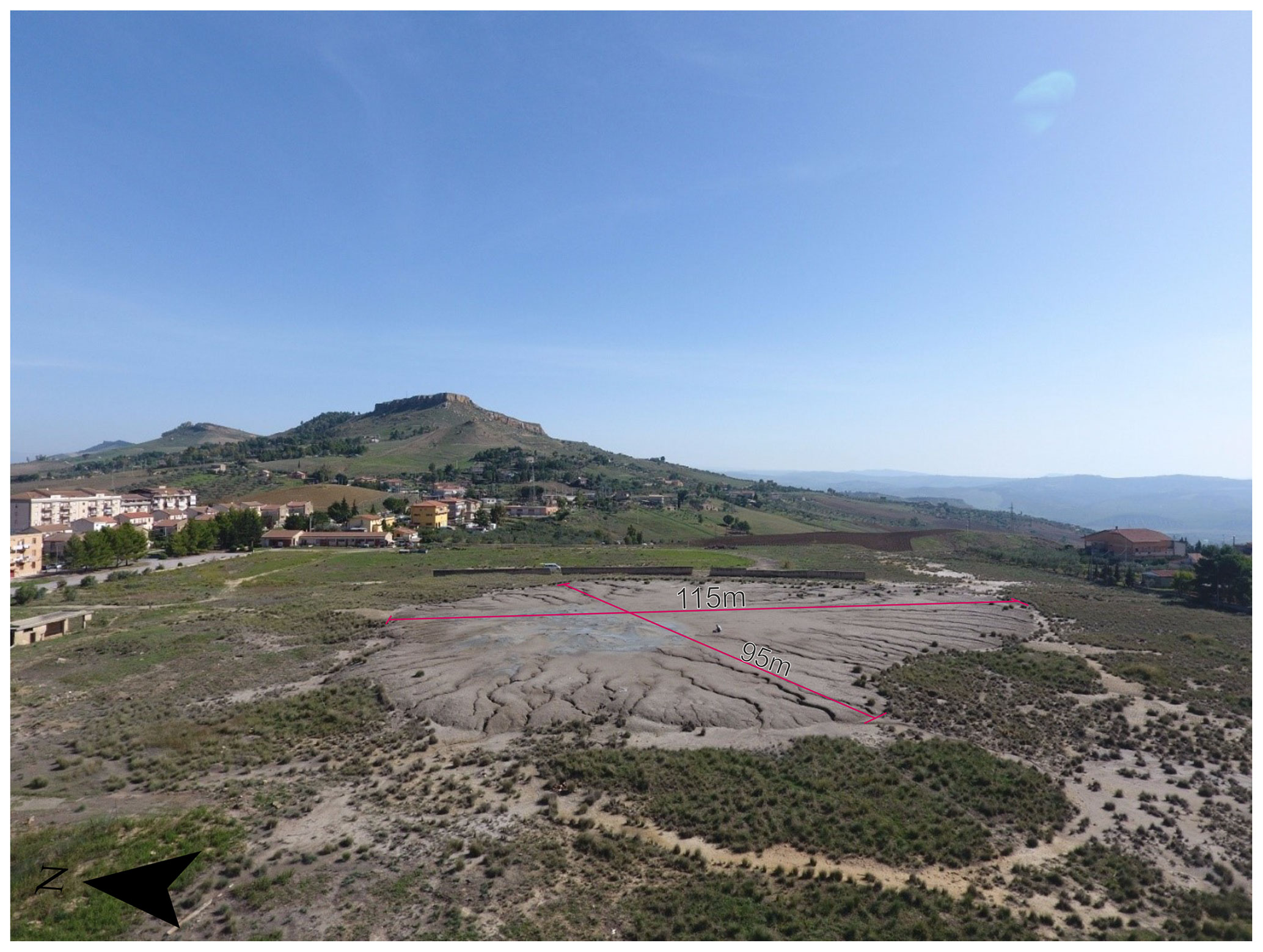
Figure 1Aerial view of the Santa Barbara mud volcano. Photo taken by the UAV from the west side of the mud volcano.
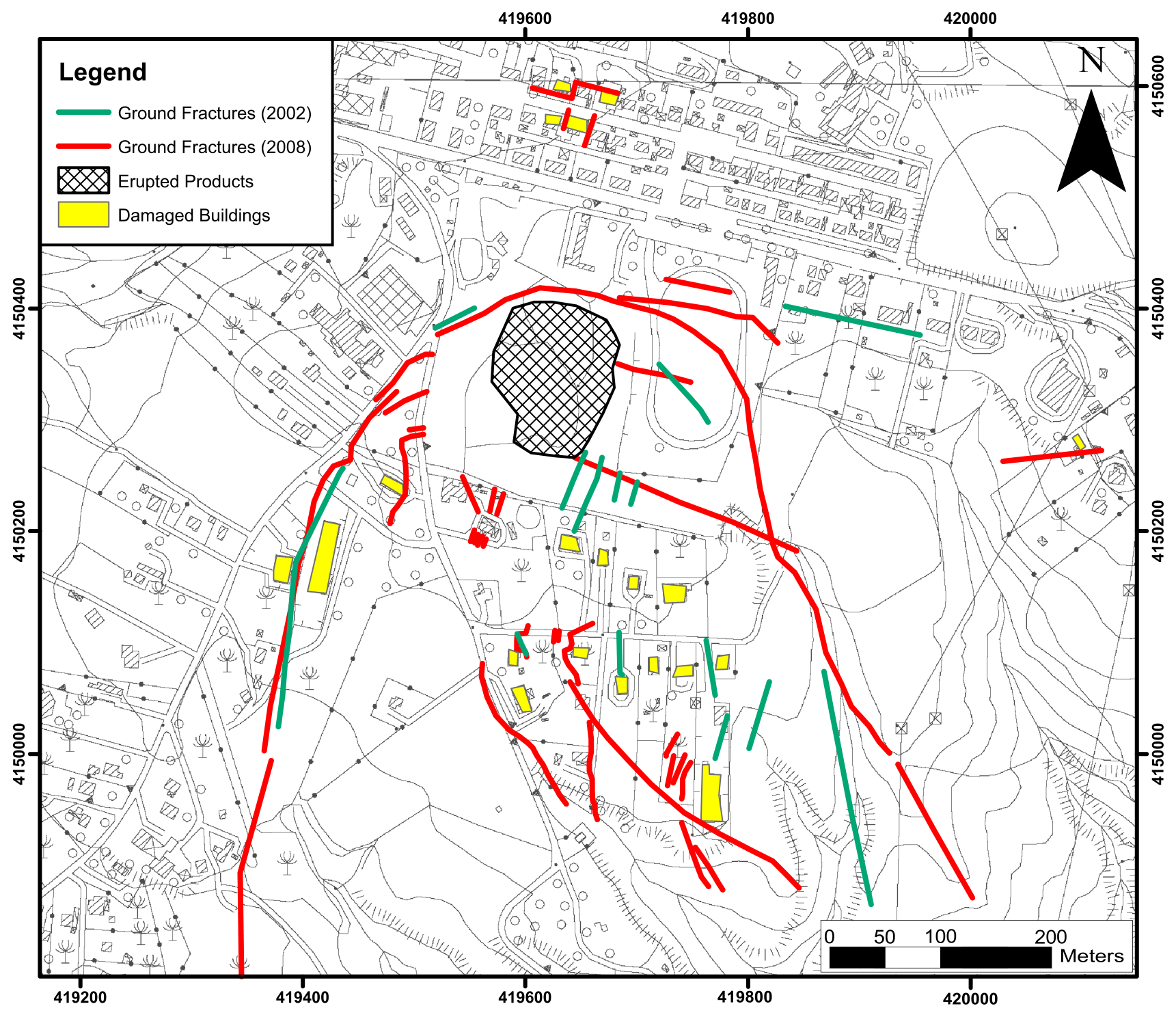
Figure 2Cartographic extract with the location of the major fractures (in red) detected on the ground and the damaged structures (in yellow) related to the paroxysmal event of 2008. In green are fractures detected in 2002. The base map is Carta Tecnica Regionale 2008 (CTR). The reference system is WGS 84/UTM zone 33N.
The mud volcano of Santa Barbara is located within the Caltanissetta foredeep basin of the Apennines–Maghrebian collisional chain which developed from the late Miocene to the Quaternary along the border of the converging Eurasia–Nubia plate (Catalano et al., 2008; Dewey et al., 1989; Serpelloni et al., 2007). This structural domain is formed by a foreland fold and thrust belt involving the deposition of clastic sediments which were gradually deformed from the late Miocene to the Pleistocene (Monaco and Tortorici, 1996; Lickorish et al., 1999, and references therein).
According to Madonia et al. (2011) mud volcanoes are most of the time in stasis, but they represent a preferential way for rising fluids rich in methane and sludge; therefore they can be considered a risk to urbanized areas or sites with an economy dedicated to natural attractions.
At several mud volcanoes (e.g., Ayaz-Akhtarma and Khara Zira island mud volcanoes in Azerbaijan), certain geomorphic and/or structural features have been observed within the year preceding a paroxysmal event (Antonielli et al., 2014; Madonia et al., 2011). The area of the Santa Barbara volcano was also affected in 2008 by a paroxysmal mud eruption which was preceded by deformation features (Fig. 2). Moreover, the surface of the mud volcanic cone is incised by a drainage system (Fig. 1) characterized by hydrographic basins with elongated dendritic geometry arranged for a centrifugal development from the areas of the summit craters towards the lower slopes of the volcano complex. The higher order of the thalwegs presents deep recessed meanders (landscape rejuvenation process). This morphometric structure is typical of uplifting areas and therefore relative decrease in the base level. This suggests an inflection process of the volcano ground surface induced by an increase in fluid pressure inside of a shallower stagnation chamber which is located at a depth of about 30 m (Imposa et al., 2018). The stagnation chamber has a “sill-like” geometry, a radius of about 50 m and a thickness of about 30 m. This morphostructural configuration supported by geophysical data configures the active geological structure as a high potential geological hazard.
On the surface, fractures and shear lineaments extend outside the erupted mud area (Madonia et al., 2011; Bonini et al., 2012; INGV, 2008; Regione Siciliana, 2008), and they highlight the high stress and strain environment induced by the mud volcano (Fig. 2). Such structures have been detected in 2002 and 2008, and we speculate that they are still active (Fig. 2). This development has often been a precursor of paroxysmal events such as the 11 August 2008 event (INGV, 2008; Regione Siciliana, 2008).
2.1 Local network
In order to monitor active deformation in the mud volcano area, a local global navigation satellite system (GNSS) network was created according to the criteria described by De Guidi et al. (2017), in particular ensuring (i) the basic requirement of spatial and temporal stability, (ii) absence of possible gravitational instabilities in both static and dynamic conditions at sites, and (iii) a panoramic and elevated position for the theodolite total station (TST).
According to these criteria two GNSS benchmarks were created, CTN0 and CTN1, located on the roof of a building in the northern sector of the studied area (Fig. 3).
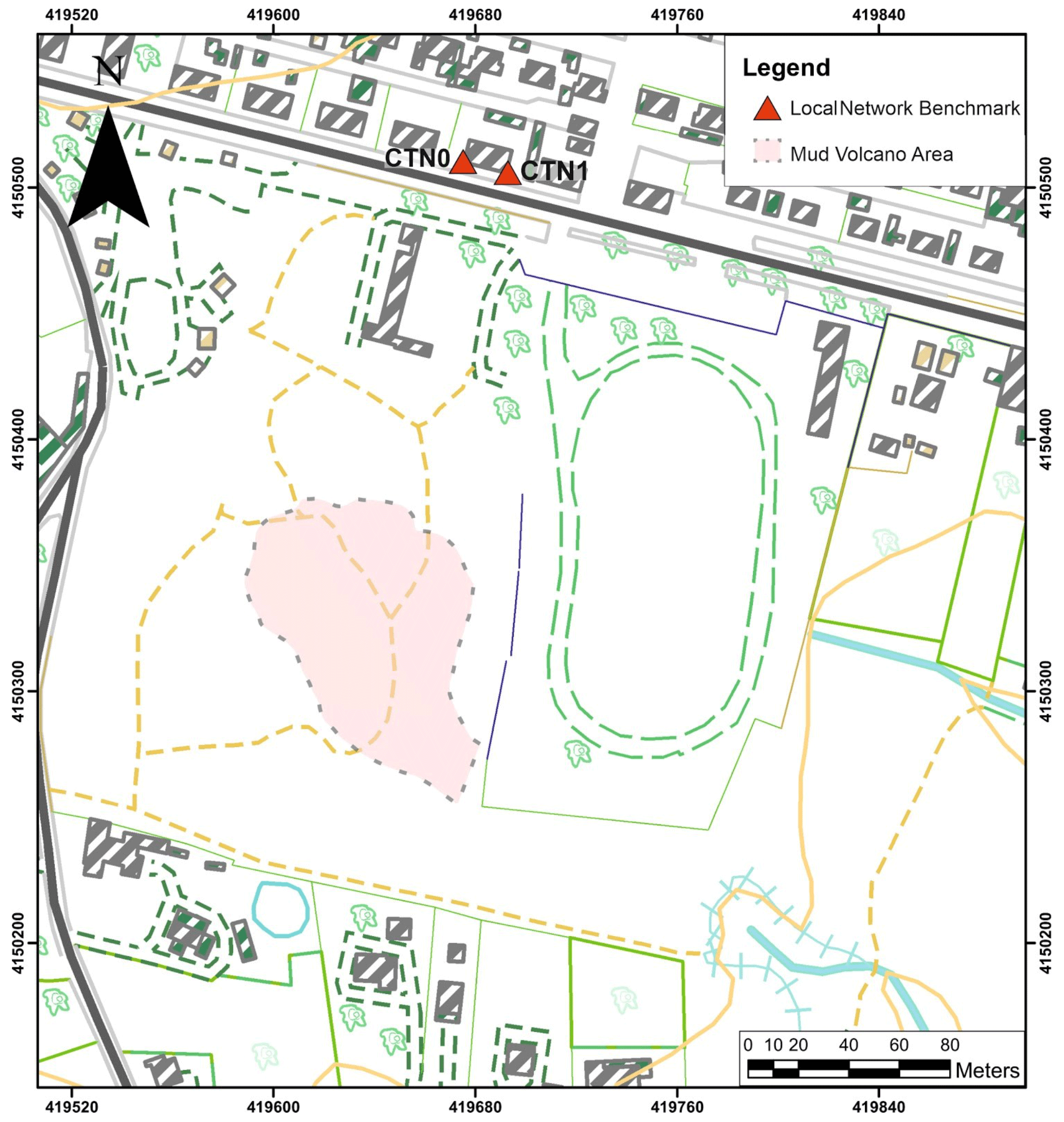
Figure 3Chorography of the eastern periphery of the inhabited area of Caltanissetta (Santa Barbara Village). The base map is Carta Tecnica Regionale 2008 (CTR). The reference system is WGS 84/UTM zone 33N.
The benchmarks were surveyed using double frequency (L1/L2) receivers (Topcon HiPer V and HiPer SR) in static mode. Once the stability of the benchmarks has been assessed, we surveyed CTN0 and CTN1 five and two times, respectively.
Post-processing of GNSS data was carried out by AUSPOS online service (Geoscience Australia, 2011; Jia et al., 2014).
To process the CTN0 data of the 28 February 2018 survey, AUSPOS used 15 International GNSS Service (IGS) stations to compute the baselines – ANKR, BOR1, BRUX, BUCU, GANP, GRAS, GRAZ, LROC, MAT1, MEDI, SOFI, TLSE, VILL, YEBE and ZIM2 – with an average ambiguity resolution of 90.0 %; position uncertainties (95 % C.L., confidence level) are respectively 0.005, 0.005 and 0.016 m for east, north and ellipsoidal height.
To process the CTN1 data of the 26 November 2018 survey, AUSPOS used 15 IGS stations to compute the baselines – ANKR, BOR1, BRUX, BUCU, GANP, GRAS, GRAZ, LROC, MAT1, MEDI, SOFI, TLSE, VILL, YEBE and ZIM2 – with an average ambiguity resolution of 84.5 %; position uncertainties (95 % C.L.) are respectively 0.007, 0.007 and 0.024 m for east, north and ellipsoidal height.
Finally, the optimal ITRF2014-UTM33N coordinates have been definitively assigned to CTN0 and CTN1.
Table 1Average RMSE of GCPs obtained for each survey and for each technique used to determinate the GCPs coordinates: X (easting), Y (northing), Z (altitude) and the total error. The image residual (“Img error” in the table) is shown.
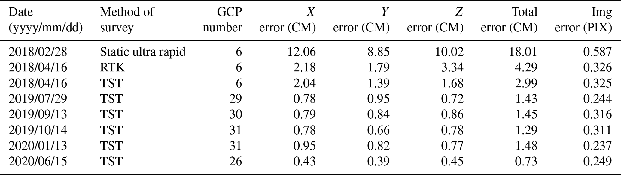
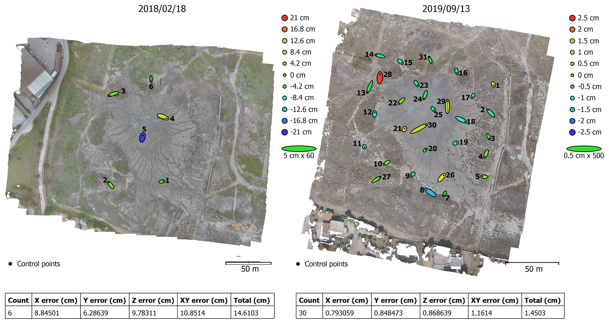
Figure 4GCPs locations and error estimates. Z error is represented by the color of the ellipse. X and Y errors are represented by ellipse shape. GCP locations are marked with a dot. Note that the different scale of the error ellipse in green: in the left image the ellipse in X direction is enlarged 60 times, and in the right image it is enlarged 500 times. The reference system is WGS 84/UTM zone 33N.
2.2 Ground control points (GCPs)
Various acquisition methods of ground control points (GCPs) were tested in order to define the most suitable one. The main function of GCPs is to georeference outcomes from SfM.
Initially (2016–2018) we used only GNSS receivers in different configurations: real-time kinematics (RTK) and static ultra rapid. The GCPs were made of 50 cm × 50 cm alveolar polypropylene square targets. Using these configurations (Table 1), errors ranging from centimeters to decimeters were recorded. In these early phases, errors were only computed by the SfM software PhotoScan (v 1.4.5.7554).
PhotoScan provides different types of error estimation: XY error (m) – root mean square error for horizontal coordinates for a GCP location; Z error (m) – error for elevation coordinate for a GCP location; error X, Y and Z (m) – root mean square error for X, Y and Z coordinates for a GCP location; error img (pix) – root mean square error for X and Y coordinates on an image for a GCP location averaged over all the images; and total error (m) – implies averaging over all the GCP locations.
Using static ultra rapid mode, the total error was about 18 cm, whereas using the RTK configuration the total error was reduced to approximately 4 cm (Brighenti et al., 2018).
From 2018 the use of the Topcon DS-103 TST was introduced, obtaining lower values for the GCP errors than those measured with the GNSS technique (Table 1). With this measurement technique the total error has been reduced to about 3 cm. On the first three campaigns, we used six GCPs to georeference the cloud points (Fig. 4). In the following section, these first three campaigns will not be considered in the computation of the significant changes for their incomparability with the last campaigns. Since 2019, we preferred to use only the TST for the GCP survey, and, according to Tahar et al. (2013), the number of GCPs has been increased (Table 1). Considering these two improvements, the total error has been reduced to about 1.4 cm and in the last campaign about 0.7 cm.
In the last two campaigns we used the TST to obtain the coordinates of the GCPs. The TST was positioned on the CTN0 point of the local network (Fig. 3) which coincides with the roof of the nearby private houses in the northern part (Fig. 5a). A classic celerimetric survey was carried out.
The measurements of the GCPs were carried out with a surveying ranging rod equipped with a reflecting prism (offset of −30 mm) assisted by a tripod with a spirit level (Fig. 5b) to ensure the upright and stability of the measurement.
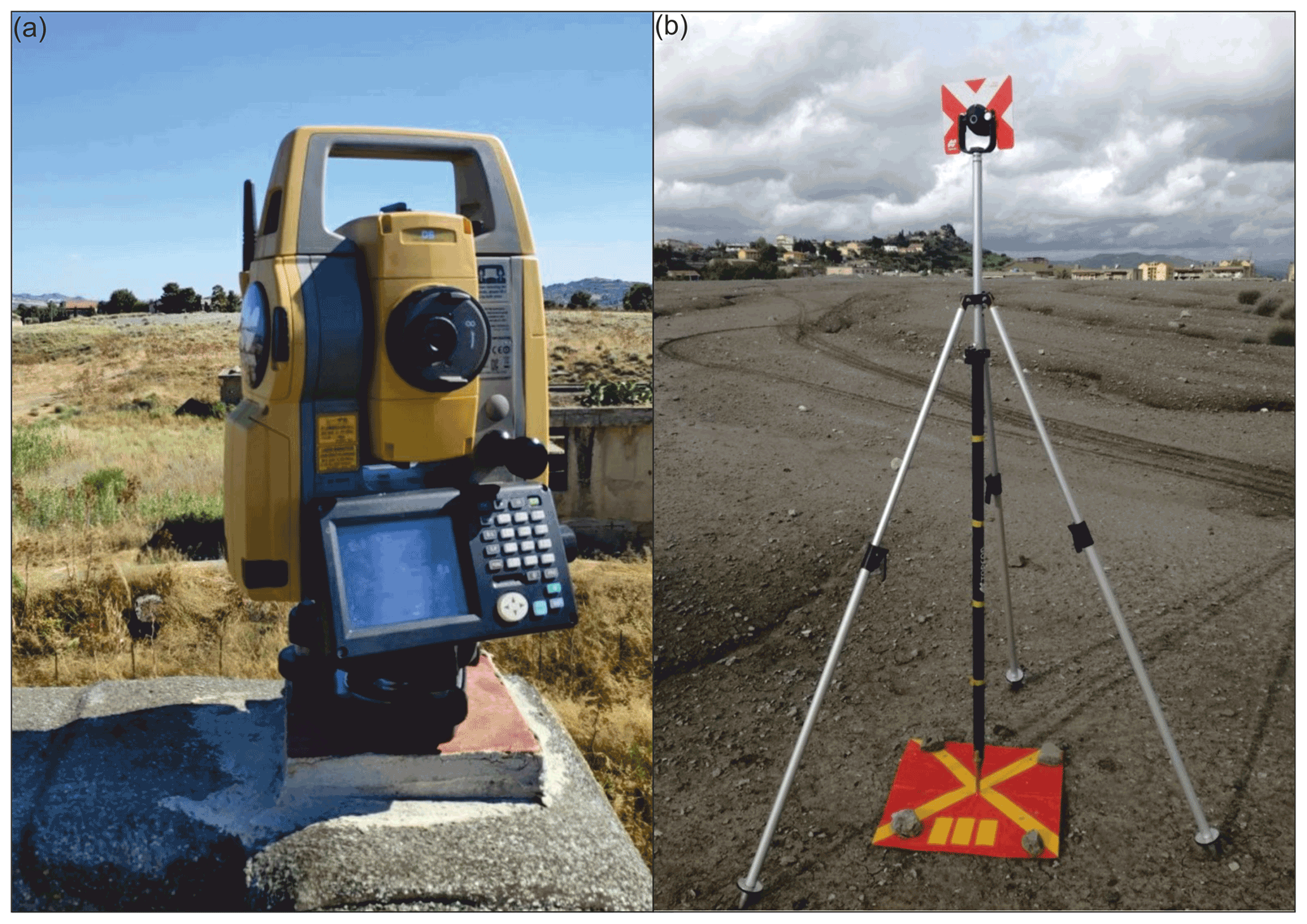
Figure 5(a) TST DS 103 placed on the fixed metal base in coincidence with point CTN0. (b) Surveying ranging rod on the mud volcano during the survey phase.
We assumed a “marker accuracy” on PhotoScan of 5 mm due to the instrumental error. This value has been assumed due to the uncertainty of the CTN0 and CTN1 point coordinates, obtained through GNSS measurements, considering that the uncertainty derived from the TST is negligible.
To validate GCP data we performed an analysis using the python script “Monte_Carlo_BA.py”, with a statistical iterative approach (Monte Carlo approach) (James et al., 2017a). For clarity, the following terminology will be used in the text:
-
GCPs are the points measured in the field. They can be used as control points or check points within the bundle adjustment (James et al., 2017a).
-
Control points are GCPs when they are tied to the model in the bundle adjustment.
-
Check points are GCPs when they are not tied to the model in the bundle adjustment.
This script modifies the percentage of GCPs which are used as check points or control points and applies to the check points random variations (James et al., 2017a). To be more precise values ranging from 10 % up to 80 % of GCPs have been set.
2.3 Photo acquisition
We have performed five measurement campaigns in approximately 1 year. The same flight plan was used for all five of them. The AOI (area of interest) was captured by a DJI Phantom 4 Standard, a quadcopter UAV, at a flight height of 33 m above the ground. The sensor size of the UAV's digital camera is 6.17 mm by 4.55 mm, capable of shooting images with a resolution of 12 MP (4000 × 3000 pixels) with a mechanical shutter. Each flight planning was carried out with the Pix4D Mapper software, adopting a frontal and side overlapping of 80 % and 70 %, respectively. The camera was set up in a nadir orientation to capture vertical imagery. The flight was carried out in a single grid (simple geometric flight patterns without intersections). An average of 280 images for each survey were acquired with about 1.1 cm ground sampling distance (GSD).
2.4 Data processing through structure from motion (SfM) techniques
The photogrammetric processing was performed using the commercial software Agisoft PhotoScan. The photogrammetric processing is based on the workflow formulated by the USGS (2017). Steps of the processing chain regarding tie point accuracy and marker accuracy have been performed according to James (2017a) (Fig. 6).

The procedure above is conventional, but we modified some parameters during the cleaning procedure of the sparse point cloud. We adopted the optimal values defined on the workflow (Fig. 6) of “reconstruction uncertain” and “projection accuracy” in the “gradual selection” option in PhotoScan. The “reconstruction uncertain” improves the geometric reconstruction of the cloud point. The “projection accuracy” improves pixel mismatches in images.
Thus, the obtained cleaned sparse cloud point was tied to the GCPs in order to georeference it.
We perform the “gradual selection” option, adjusting the “reprojection error” values to reduce the residual pixel errors (Fig. 6) (USGS, 2017).
Furthermore, appropriate pixel values of tie point accuracy and marker accuracy are set following the suggestions of James et al. (2017b).
We applied the “precision_estimate.py” script (James et al., 2017b). The script operates by an interactive Monte Carlo approach to estimate the accuracy of SfM surveys through photogrammetric and georeferencing parameters, which are then used to provide spatially variable confidence limits for the detection of surface variations.
The precision estimates are calculated through multiple “bundle adjustments” (“optimize camera alignment” in PhotoScan) with different pseudo-random offsets (in this case 4000 pseudo-random offsets) (Fig. 7) applied to each image and checkpoint. The pseudo-random offsets are derived from normal distributions with standard deviations representative of the appropriate accuracy within the survey (James et al., 2017b).
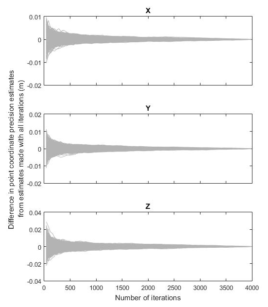
Figure 7Example of the iterative approach in the 29 July 2020 survey. Estimates of uncertainties on X, Y and Z improve as the number of iterations increase.
The SfM-Georef software (James and Robson, 2012) reads the output given by the Monte Carlo python script, setting to each point of the sparse cloud different values of precision on the three spatial components. The results of the script, read by SfM-Georef, are estimates of the error of the individual points of the sparse cloud point in the three different spatial dimensions (Fig. 8).
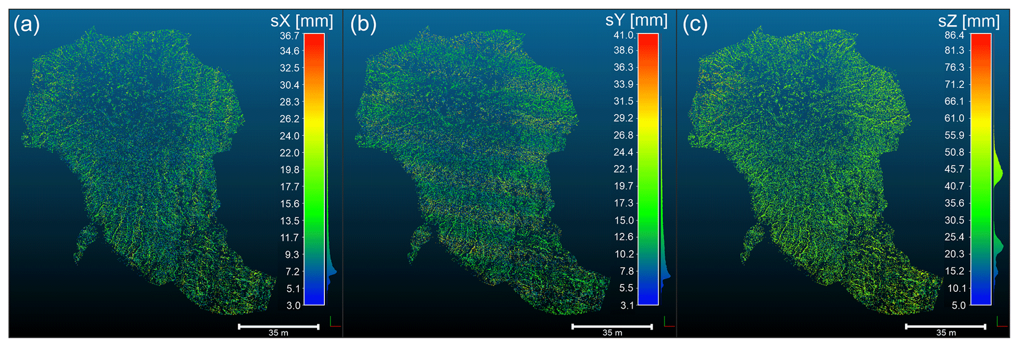
Figure 83D error estimates of each point of the sparse cloud of the 13 September 2019 survey. The error (sX, sY, sZ) is in millimeters. (a) and (b) The horizontal errors (X and Y component) are shown. (c) The vertical errors (Z component) are shown. The reference system is WGS 84/UTM zone 33N.

Figure 9Estimates of the 3D error of the dense point cloud obtained by interpolation with the sparse cloud of the 13 September 2019 survey. The error (sX, sY, sZ) is in millimeters. (a) and (b) The horizontal errors (X and Y component) are shown. (c) The vertical errors (Z component) are shown. The reference system is WGS 84/UTM zone 33N.
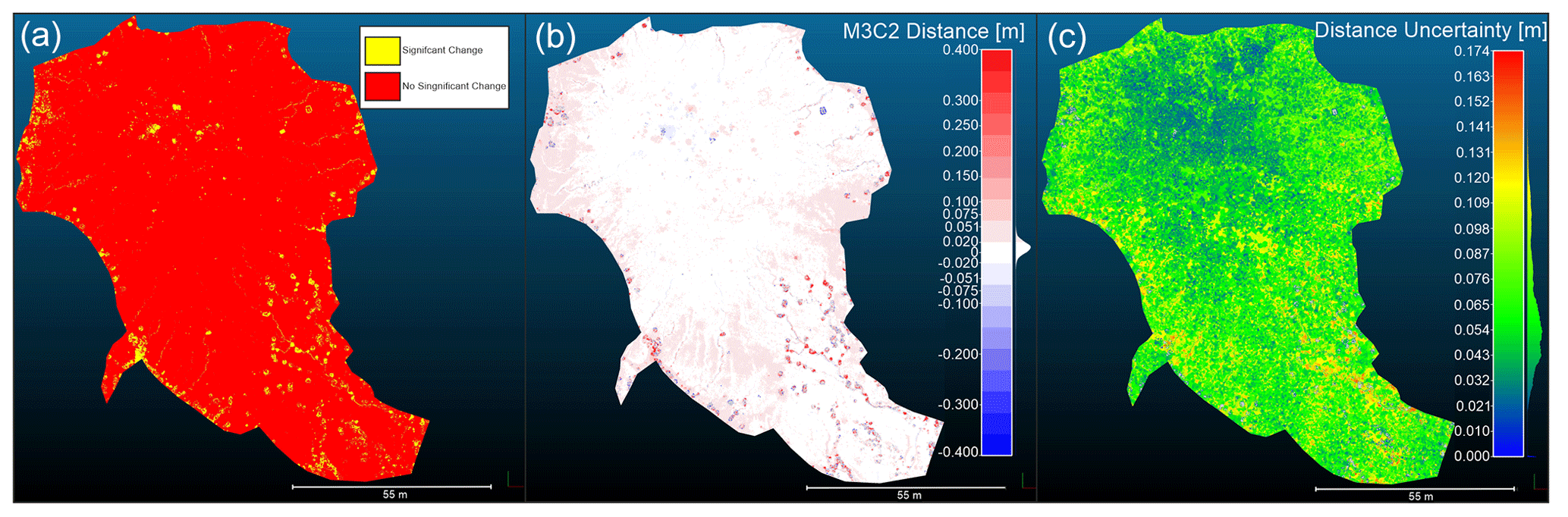
Figure 10Point clouds resulting from M3C2-PM processing – comparison between 29 July 2019 and 15 June 2020: (a) significant changes between the two point clouds with LOD% 95, (b) distances between the two point clouds and (c) uncertainty of the distance between the two point clouds. The reference system is WGS 84/UTM zone 33N.
The 3D topographic change is usually detected from sparse point clouds that have been cleaned to exclude the vegetation that interferes with the comparison techniques. The next step is to link those points to the precision estimates of the sparse cloud; this has been done in CloudCompare v. 2.11 (http://www.cloudcompare.org/, last access: 15 October 2019).
Through CloudCompare the sparse cloud is interpolated (with the relative precision values on the 3D components) with the dense point cloud. In this phase we decide which interpolation technique is the most suitable; in this case we chose the “nearest neighbors” that are the three closest points to the sparse cloud, using the median value (better outlier mitigation) to assign the error values to the dense point clouds (Fig. 9). This methodology has been chosen due to the heterogeneous distribution of the points in the sparse cloud, avoiding points with null values.
Once the precise dense point cloud and their error have been obtained, it is possible to compare the surveys in order to determine the changes between them. Comparisons between the surveys were performed on CloudCompare by the M3C2-PM plugin (James et al., 2017b; Lague et al., 2013) that identifies a statistically significant change where the topographical differences exceed a value of spatially variable uncertainty. According to James et al. (2017b), the M3C2-PM is particularly suited for point clouds derived from SfM. The M3C2-PM (James et al., 2017b) uses estimates of the precision of the coordinates of points (3D precision map) that we have previously calculated.
The outputs of M3C2-PM are scalar values applied to the cloud:
-
significant change (Fig. 10a)
-
M3C2 distance (Fig. 10b)
-
distance uncertainty (Fig. 10c).
The first output (Fig. 10a) shows the changes which exceed the uncertainty values in both point clouds. It represents a confidence interval constrained by values with a level of detection at 95 % confidence (LoD95 %) which are spatially variable. This is applicable in any morphological setting, providing a reliable 3D analysis of topographical change.
The second output (Fig. 10b) shows the calculated distances between the two clouds.
The third output (Fig. 10c) shows the uncertainty values of the distances and their spatial variation between the two clouds. Once the uncertainty value is defined, the changes are significant when they overtake the value of the uncertainty.
In the 15 June 2020 survey, we used callipers to test and validate the method of the measurements. Five numbered callipers, with steps of increasing height of about 2 cm, were positioned on the mud dome. The heights are 2, 4, 6, 8 and 10 cm.
These were used to obtain an instrumental sensitivity of the measures (Fig. 11). All callipers are detected, and we show as an example the smallest (Fig. 11).
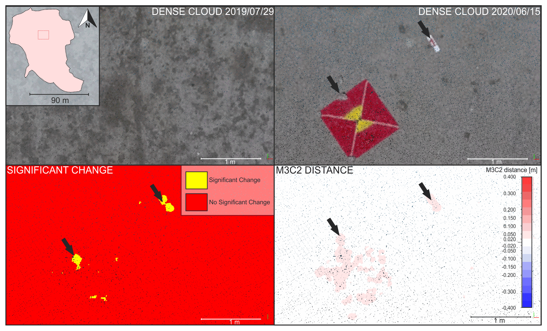
Figure 11In the upper part of the figure, the dense point clouds of the two surveys of the same area carried out on 29 July 2019 (left) and 15 June 2020 (right) are shown. In the lower part are the clouds with the significant change (left) and the M3C2 distance (right). The arrows indicate the significant changes between the surveys. The calculated changes between the two clouds estimate an altitude increase of about 6.3 cm for the fragment of rock used to maintain the target in position and an increase in height of about 2.5 cm for the calliper which is 2 cm thick. The reference system is WGS 84/UTM zone 33N.
As illustrated in Sect. 2.2, the results show that using between 40 % and 60 % of the GCPs (as control points) the RMSE value has minimal variation. Thus, the optimal minimum number of GPCs is between 12 and 18. When the threshold of 60 % is exceeded, there are no significant improvements (Fig. 12). This result has been confirmed in all campaigns.

Figure 12The boxes represent the distribution of the RMSE of GCPs (13 September 2019 survey) on the three components: magnitude (3D), horizontal and vertical according to the percentage of the GCPs used as control points. RMSE is calculated on 50 self-calibrating bundle adjustments for each percentage of GCPs used as control points. The GCPs are randomly selected for each self-calibrating bundle adjustment. The central bars indicate the median RMSE values, which are included in the boxes that extend from the 25th to 75th percentile, and the outliers are indicated by the + symbols.
The results obtained from the photogrammetric comparisons supported by geodetic topographic survey have an average uncertainty of about 6.4 cm, with a minimum of about 2 cm and a maximum of about 12 cm, relative to an area of 42 700 m2 (Fig. 13a). The uncertainty of the central area has an average value of about 3.9 cm, with a minimum of about 2 cm and maximum of 10 cm, on an extension of 360 m2 (Fig. 13b).
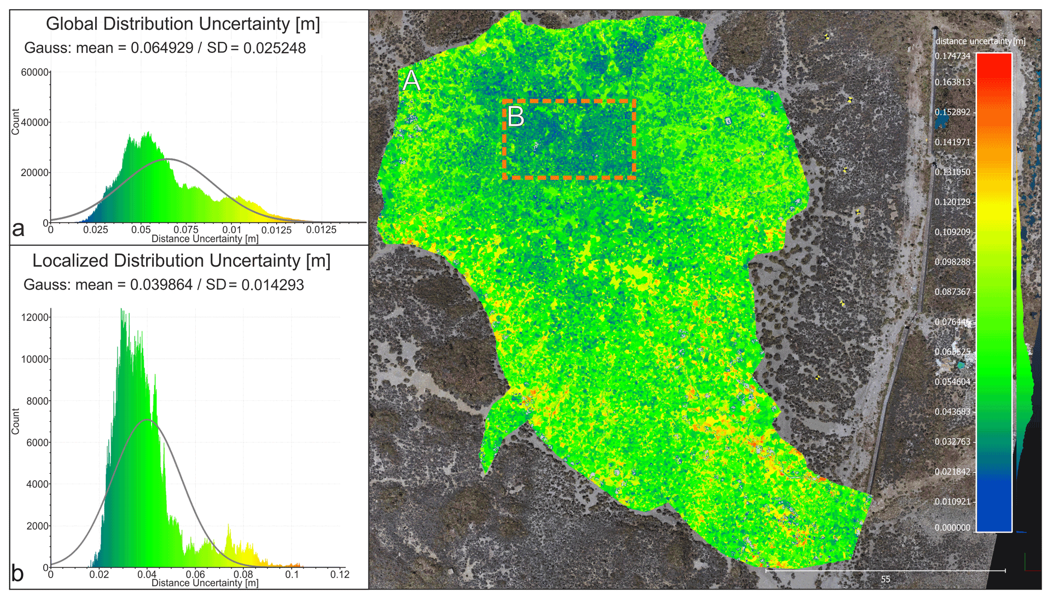
Figure 13Point clouds with uncertainty distance values between 29 July 2019 and 15 June 2020 (right). On the left, (a) the Gaussian distribution of the distance uncertainty over the whole area is shown; the mean is about 6.4 cm, and the standard deviation is about 2.5 cm. (b) The Gaussian distribution of the distance uncertainty of the central emission area is shown; the mean is about 3.9 cm, and the standard deviation is about 1.4 cm. The reference system is WGS 84/UTM zone 33N.
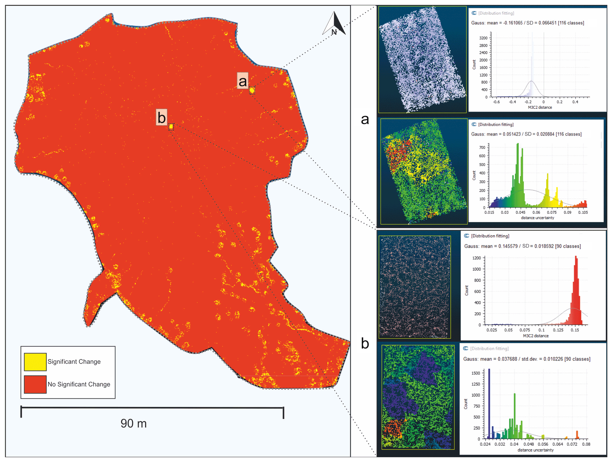
Figure 14Enlargement of the comparison between the point clouds of the 13 September 2019 and 14 October 2019 campaigns with significant changes. Two significant changes (a and b) are shown, which highlight an anthropogenic action, i.e., the movement of a wooden platform about 15 cm high. (a, upper part) A lowering of an average height of 16 cm is detected, and the Gaussian distribution of the M3C2-PM distances with the mean and the standard deviation is shown. (a, lower part) The distance uncertainty varies spatially with an average value of about 5 cm, and the Gaussian distribution of the M3C2-PM distances with the mean and the standard deviation is shown. (b, upper part) An increase in height of 14 cm is recorded, and the Gaussian distribution of the M3C2-PM distances with the mean and the standard deviation is shown. (b, lower part) The distance uncertainty has an average value of about 3 cm, and the Gaussian distribution of the M3C2-PM distances with the mean and the standard deviation is shown. The reference system is WGS 84/UTM zone 33N.
During the monitoring period, in addition to natural changes, we recorded anthropogenic action due to the relocation of objects (garbage) in the area after unauthorized access. These changes have a decimetric order of magnitude and are easily detected by the technique used (Fig. 14).
Two types of analysis were carried out: semi-quantitative and quantitative. The surveys on 29 July 2019 and 15 June 2020 (time interval of about 1 year) were chosen to perform the semi-quantitative analysis. This analysis was carried out on the whole mud volcano area, and the objective is to detect significant deformations (on the order of decimeters). In order to visualize this deformation (Fig. 15), the values of M3C2 distance ranging between −2 and 2 cm were excluded according to the minimum value of distance uncertainty. This range was verified instrumentally with the use of callipers.

Figure 15Orthophoto with M3C2 distance. The distance scale has been adjusted to exclude values between −2 and +2 cm. The positive distances, observed at the margin of the mud dome, are interpreted as mud flow or sediment deposition coming from peripheral griffon vent eruptions or erosion of summit area. The reference system is WGS 84/UTM zone 33N.
Comparing the 29 July 2019 and 15 June 2020 surveys (Fig. 15), we observe that the surface of the volcanic cone is not affected by deformations. Only morphological changes in the volcanic structures can be underlined, such as small eruptive cones, gryphons, sauces and mud pools.
The quantitative analysis was performed on small central portions of the mud volcano. The aim of the quantitative analysis is to estimate the trend and evolution of the deformation. To assess the deformation and the local morphostructural evolution, two temporal series have been developed in two areas: Z1 (collapse zone) and Z2 (uplifting zone) (Figs. 16 and 17). The zones were chosen in relation to the significant change. For the selected zone, the average distances between points with significant change were computed by M3C2-PM. Z1 has an extension of 1 m2 (Fig. 16), and Z2 has an extension of 0.84 m2 (Fig. 17).
The campaign of 29 July 2019 (T0) was chosen as the master (Table 2).
Table 2Surveys used to generate the time series. Dates are given in yyyy/mm/dd.

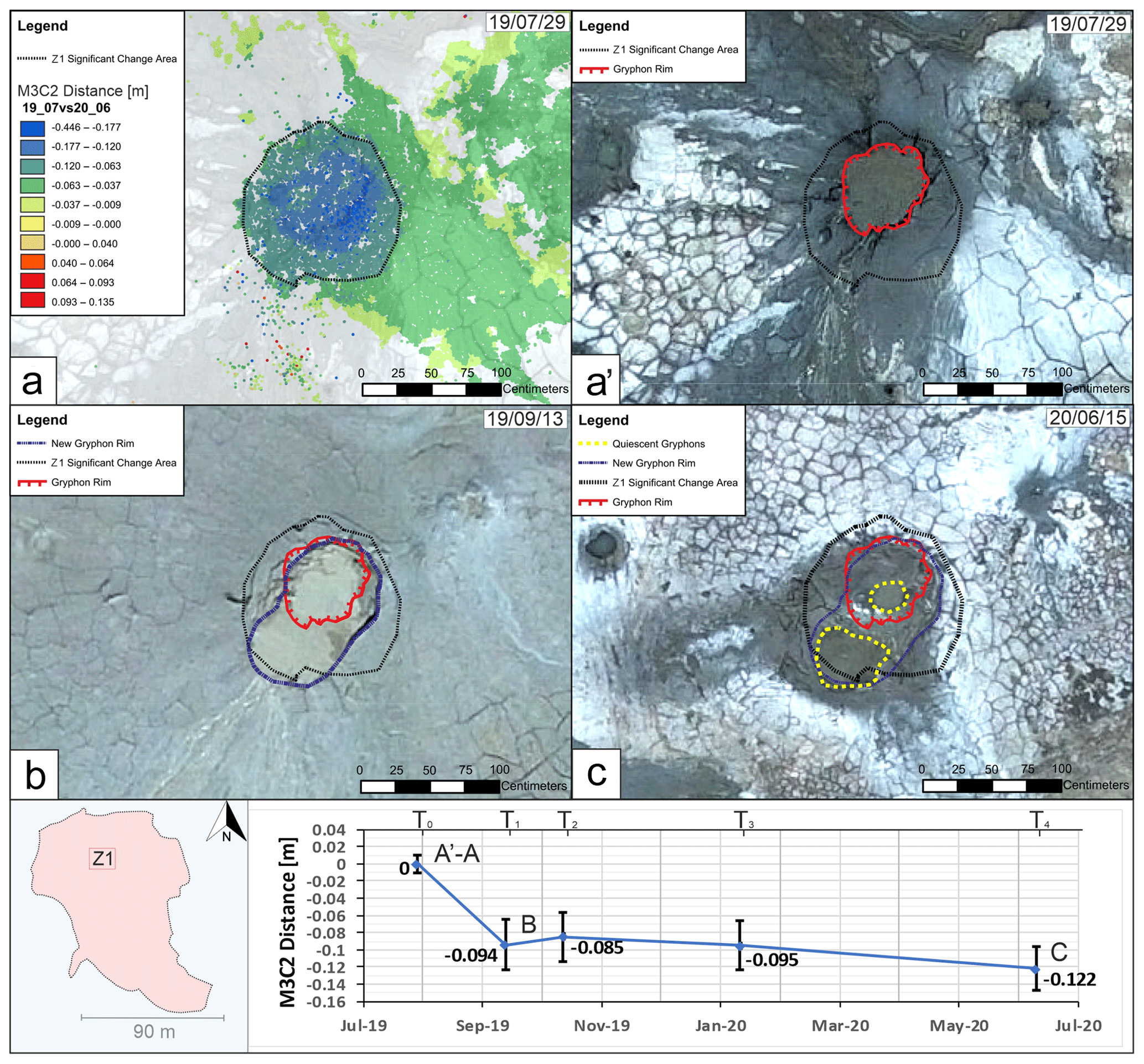
Figure 16(a) M3C2 distance (29 July 2019 vs. 15 June 2020) of Z1; the area used to create the time series is delimited with a dashed line (selected by significant change). (a') Orthophoto of 29 July 2019 with the gryphon border in red. (b) The orthophoto of 13 September 2019 highlights the expansion of the gryphon border in blue. (c) Orthophotos of 15 June 2020 showing the gryphon during the quiescence phase and the split of the channel in yellow. Below, the time series with a decreasing trend is shown. The reference system is WGS 84/UTM zone 33N.
In Fig. 16, the subsidence (about 10 cm per 60 d) of gryphon is represented by the southwest migration of the mud pool edge. In Fig. 17, the uplift (about 4 cm per 60 d) of a blind gryphon is represented by the development of radial fractures on the cone surface. Close to the growing gryphon, another indication of deformation is the deviation of a mudslide flowing in the north–south direction towards the southern sector of the analyzed area. Finally, the sudden appearance of the gryphon is well highlighted in the orthophoto of the last survey (Fig. 17).
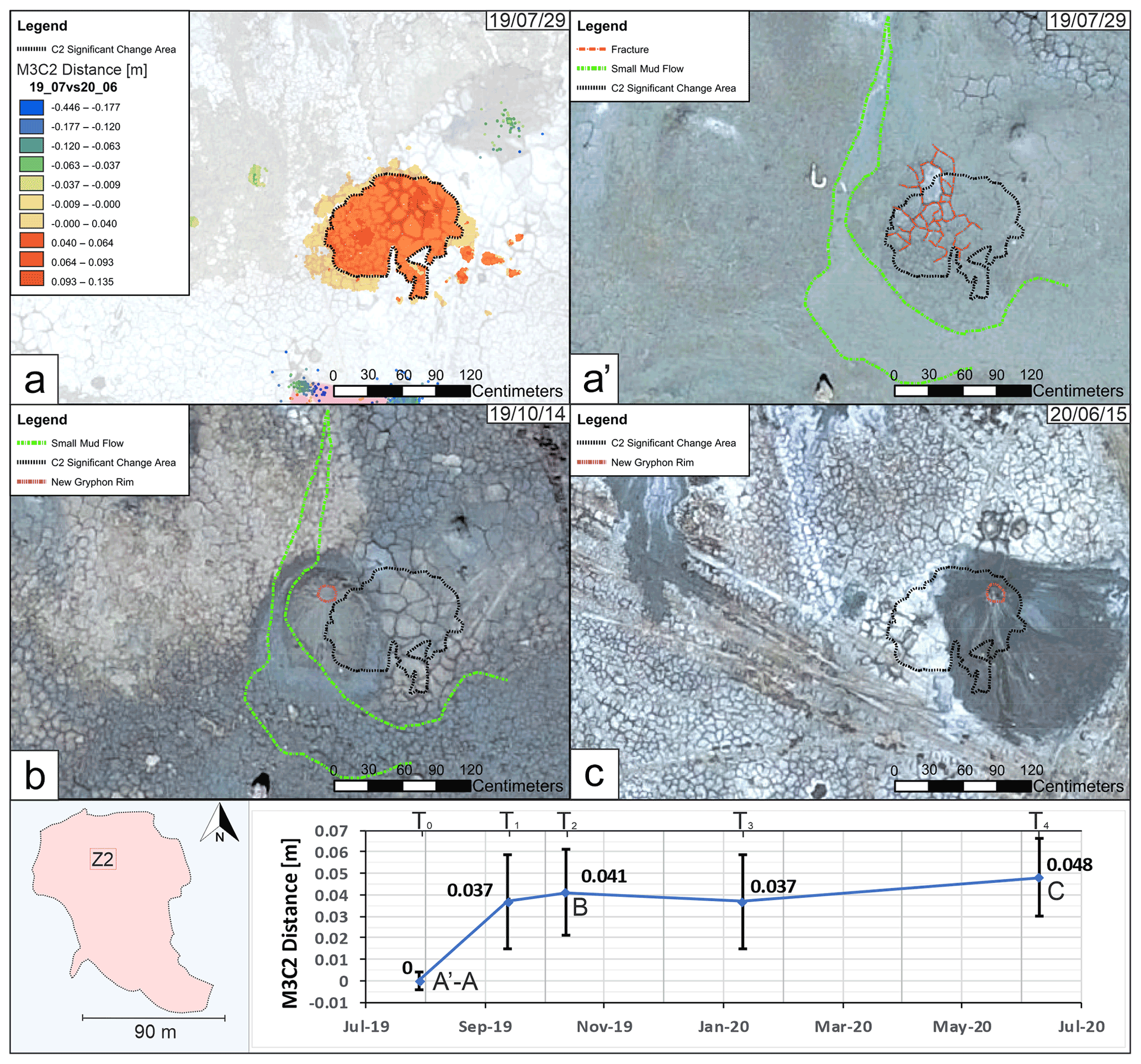
Figure 17(a) M3C2 distance (29 July 2019 vs. 15 June 2020) of the Z2; the area used to create the time series is delimited with a dashed line (selected by significant change). (a') Orthophoto of 29 July 2019, the margin of the deflected flow in green and the radial fractures in red. (b) Orthophoto of 14 October 2019, formation of a new emission gryphon in red and the previous flow in green. (c) Orthophoto of 15 June 2020, formation of a new emission gryphon in red. Below, the time series with upward trend is shown. The reference system is WGS 84/UTM zone 33N.
UAV technology combined with SfM is a valuable tool in geological risk assessment and monitoring; however, some issues must be considered.
The first is the quantity and quality of the acquired GCPs. According to the results, the minimum optimal number for georeferencing is 12 GCPs. A slight improvement is observable up to 18 GCPs, while no appraisable improvement is detected for a higher number of GCPs (Fig. 12). In addition, the method of acquiring GCPs reduces their error by using the total station theodolite (Table 1). The combined use of high-precision topographic instruments with an optimal number of GCPs improves the reliability of the datasets.
The second aspect to be considered is the evaluation of distance uncertainty when two surveys are compared. The distance uncertainty between two datasets (surveys) can be considered as an estimate of the sensitivity of the methods to detect measurable topographic changes. The results of the M3C2-PM show that the average distance uncertainty between the first and the last surveys is about 6.5 cm over the whole area at the 95 % confidence level (Fig. 13a). Furthermore, considering a smaller portion of the area, the uncertainty decreases to about 3.9 cm at the 95 % confidence level (Fig. 13b). This allows us to analyze certain morphological changes and anthropogenic activity on the mud surface (Fig. 14). The anthropogenic activity determined a height decrease of about 16 cm where a wood platform was previously located. Moreover, a height increase of about 14 cm is recorded at the place where the wood platform has been relocated. The values recorded are consistent with the real thickness of the object detected, differing by 2 cm (Fig. 14). The callipers show that it is possible to measure changes of at least 2 cm (Fig. 11).
After the uncertainty and sensitivity of the surveys were computed, the time series were made. Considering the significant changes and their errors, we computed the trend of deformation of two areas in order to reconstruct the evolution of the phenomena which generated these changes (Figs. 16 and 17).
Considering the results obtained by SfM, we propose a monitoring system of the Santa Barbara mud volcano based on a semi-quantitative approach. We defined three states by setting a space-time range:
-
normal state if the deformation value does not exceed 5 cm in the range between 1 and 2 months
-
pre-alert state if the deformation value is between 5 cm and 10 cm during a period of between 1 and 2 months
-
alert state if the deformation value exceeds 10 cm in the range between 1 and 2 months.
To define the state of the activity of the mud volcano, the area affected by deformation must be a significant area of the total surface of the volcano. The definition of the activity is an important aspect of the monitoring of hazard because there are many natural phenomena that can produce deformation in a small area (like a gryphon) or in a larger portion (like the sedimentation occurring at the border of the mud volcano). The significant area affected by deformation must be correctly defined by an operator (public agency, university, institute of research or Dipartimento della Protezione Civile) which really knows the natural phenomena that can occur on the Santa Barbara mud volcano.
The methodological approach is valuable and efficient from the point of view of quantity and quality of data collected in relation to the work and time spent. This monitoring technique is a useful tool to detect the early unrest phase of the mud volcano usually induced by changes in pressure and volume of fluid rising from the stagnation chamber.
The pre-eruptive deformation consists of a marked uplift and occasional small subsidence which are probably related to the redistribution of the subsoil of the pressurized fluids (Antonelli et al., 2014). According to Antonelli et al. (2014), soil uplift can occur up to a year before the eruption.
In hazard management, the SfM technique (Gomez and Purdie, 2016; Kaab, 2000; Fugazza et al., 2018; Giordan et al., 2017, 2018) is starting to be widely used by the scientific community. In the monitoring of potentially dangerous active sites, the UAVs are very advantageous because they are not used only as a support in the post-disaster events (Rokhmana and Andaru, 2017; Hisbaron et al., 2018) but also for the pre-event monitoring.
According to Kopf (2002), Antonielli et al. (2014), Madonia et al. (2011), INGV (2008), and Regione Siciliana (2008), the deformations of the surface shell of mud volcanoes can occur up to 1 year before the paroxysmal event with doming and the development of structural lineaments with an order of magnitude from centimeters to decimeters.
The results allow us to define the criteria for monitoring and analyzing the study area. For the mud volcano of Santa Barbara, the monitoring criteria are as follows:
-
Monitoring interval is between 1 and 2 months.
-
The optimal number of GCPs is between 12 and 18.
-
Acquisition of GCPs is by high-precision topographical instrumentation (TST).
-
The processing chain of the sparse point cloud according to workflow of USGS (2017) was enhanced by the correct value of “tie point accuracy” and “marker accuracy” as suggested by James (2017a).
-
An assessment of the state of activity of the mud volcano is based on a semi-quantitative approach.
The frequency of the campaigns depends on the status of activity, while the other criteria depend on the object/structure of the monitoring.
These criteria allow us to detect events with deformation of at least 2 cm. In the case of anomalous values detected, the monitoring campaigns must be improved. This involves extensive monitoring, such as (i) developing time series localized in key areas and (ii) combining different methodologies, e.g., micro-seismicity monitoring and 3D geophysical prospecting (Imposa et al., 2016), to improve the monitoring system of the active geological process.
The codes used in this paper are provided by authors cited in the text. The links to these codes or software are as follows: Precision_estimates.py: https://www.lancaster.ac.uk/staff/jamesm/software/python/pe_1.4.0/precision_estimates.pySfm_georef (James, 2018), http://www.lancaster.ac.uk/staff/jamesm/software/sfm_georef.htmMonte_Carlo_BA.p (James, 2017b), https://www.lancaster.ac.uk/staff/jamesm/software/python/gcp_1.3.0/Monte_Carlo_BA.py (James, 2016).
The data are available on request by email to the corresponding author (giorgio.deguidi@unict.it) and to Fabio Brighenti (fabio.brighenti@unict.it).
FB conducted the photogrammetric processing and all the statistical analysis of the point clouds. DM and GDG conducted the UAV flight campaigns. FB, FC, DM and GDG conducted the topographic and geodetic surveys. FC conducted the GNSS processing and analysis. FB and FC conducted the topographic processing and analysis. FB, FC and GDG wrote the paper. FB produced the figures. GDG was the supervisor. All the authors were involved in the conceptualization, discussion of the results and editing of the manuscript.
The authors declare that they have no conflict of interest.
Publisher’s note: Copernicus Publications remains neutral with regard to jurisdictional claims in published maps and institutional affiliations.
This article is part of the special issue “Remote sensing and Earth observation data in natural hazard and risk studies”. It is not associated with a conference.
We thank Silvia Rita Popolo for her valuable support. Finally, we are gratefull to the two anonymous referees and to Elena Russo who helped us to enhance the clarity and structure of the content of this manuscript.
This research has been supported by the Presidenza del Consiglio dei Ministri (Project Code E98D19000000001, Monitoraggio e Studio dei Processi di 10 Deformazione Superficiale Connessi al Vulcanismo-Sedimentario delle Maccalube di Santa Barbara (Caltanisetta) within the DPCM 25 May 2016 – Riqualificazione Urbana e la Sicurezza delle Periferie delle Città Metropolitane, dei Comuni Capoluogo e delle Città di Aosta; scientific supervisor: Giorgio De Guidi). Moreover, the publication of the paper has been supported by the PhD in Earth and Environmental Sciences fund (PhD coordinator Agata Di Stefano), the PIAno di inCEntivi per la RIcerca di Ateneo (PIACERI 2020/2022) (fund manager Giorgio De Guidi) and UPC Piano Della Ricerca (fund manager Carmelo Monaco).
This paper was edited by Michelle Parks and reviewed by Elena Russo and two anonymous referees.
Amici, S., Turci, M., Giammanco, S., Spampinato, L., and Giulietti, F.: UAV Thermal Infrared Remote Sensing of an Italian Mud Volcano, Advances in Remote Sensing 2, 358–364, https://doi.org/10.4236/ars.2013.24038, 2013a.
Amici, S., Turci, M., Giulietti, F., Giammanco, S., Buongiorno, M. F., La Spina, A., and Spampinato, L.: VOLCANIC ENVIRONMENTS MONITORING BY DRONES MUD VOLCANO CASE STUDY, Int. Arch. Photogramm. Remote Sens. Spatial Inf. Sci., XL-1/W2, 5–10, https://doi.org/10.5194/isprsarchives-XL-1-W2-5-2013, 2013b.
Andaru, R. and Rau, J.-Y.: LAVA DOME CHANGES DETECTION AT AGUNG MOUNTAIN DURING HIGH LEVEL OF VOLCANIC ACTIVITY USING UAV PHOTOGRAMMETRY, Int. Arch. Photogramm. Remote Sens. Spatial Inf. Sci., XLII-2/W13, 173–179, https://doi.org/10.5194/isprs-archives-XLII-2-W13-173-2019, 2019.
Antonielli, B., Monserrat, O., Bonini, M., Righini, G., Sani F., Luzi, G., Feyzullayev, A. A., and Aliyev, C. S.: Pre-eruptive ground deformation of Azerbaijan mud volcanoes detected through satellite radar interferometry (DInSAR), Tectonophysics, 637, 163–177, https://doi.org/10.1016/j.tecto.2014.10.005, 2014.
Bakker, M. and Lane, S. N.: Archival photogrammetric analysis of river–floodplain systems using Structure from Motion (SfM) methods, Earth Surf. Proc. Land., 42, 1274–1286, https://doi.org/10.1002/esp.4085, 2015.
Balaguer-Puig, M., Marqués-Mateu, Á., Lerma, J. L., and Ibáñez-Asensio, S.: Estimation of small-scale soil erosion in laboratory experiments with Structure from Motion photogrammetry, Geomorphology, 295, 285–296, https://doi.org/10.1016/j.geomorph.2017.04.035, 2017.
Bemis, S. P., Micklethwaite, S.,Turner, D., James, M. R., Akciz, S., Thiele, S. T., and Ali Bangash, H.: Ground-based and UAV-Based photogrammetry: A multi-scale, high-resolution mapping tool for structural geology and paleoseismology, J. Struct. Geol., 69, 163–178, https://doi.org/10.1016/j.jsg.2014.10.007, 2014.
Boccardo, P., Chiabrando, F., Dutto, F., Tonolo, F. G., and Lingua, A.: UAV deployment exercise for mapping purposes: evaluation of emergency response applications, Sensors, 15, 15717–15737, https://doi.org/10.3390/s150715717, 2015.
Bonali, F. L., Tibaldi, A., Marchese, F., Fallati, F., Russo, E., Corselli, C., and Savini, A.: UAV-based surveying in volcano-tectonics: An example from the Iceland rift, J. Struct. Geol., 121, 46–64, https://doi.org/10.1016/j.jsg.2019.02.004, 2019.
Bonini, M.: Mud volcanoes: Indicators of stress orientation and tectonic controls, Earth-Sci. Rev., 115, 121–152, https://doi.org/10.1016/j.earscirev.2012.09.002, 2012.
Bretar, F., Arab-Sedze, M., Champion, J., Pierrot-Deseilligny, M., Heggy, E., and Jacquemoud, S.: An advanced photogrammetric method to measure surface roughness: Application to volcanic terrains in the Piton de la Fournaise, Reunion Island, Remote Sens. Environ., 135, 1–11, https://doi.org/10.1016/j.rse.2013.03.026, 2013.
Brighenti, F., Carnemolla, F., Messina, D., Lupo, M., De Guidi, G. and Barreca, G.: Geo-referencing techniques of 3d models (SfM): Case study of mud volcano, Village Santa Barbara, Caltanissetta (Sicily), 89∘ Congresso SGI – SIMP, Geosciences for the environment, natural hazard and cultural heritage, Catania, 12–14 September, 2018.
Brunier, G., Fleury, J., Anthony, E. J., Gardel, A., and Dussouillez, P.: Close-range airborne Structure-from-Motion Photogrammetry for high-resolution beach morphometric surveys: Examples from an embayed rotating beach, Geomorphology, 261, 76–88, https://doi.org/10.1016/j.geomorph.2016.02.025, 2016.
Carr, B. B., Clarke, A. B., Arrowsmith, J. R., Vanderkluysen, L., and Dhanu, B. E.: The emplacement of the active lava flow at Sinabung Volcano, Sumatra, Indonesia, documented by structure-from-motion photogrammetry, J. Volcanol. Geoth. Res., 382, 164–172, https://doi.org/10.1016/j.jvolgeores.2018.02.004, 2018.
Casella, E., Rovere, A., Pedroncini, A., Mucerino, L., Casella, M., Cusati, L. A., Vacchi, M., Ferrari, M., and Firpo, M.: Study of wave runup using numerical models and low-altitude aerial photogrammetry: a tool for coastal management, Estuar. Coast. Shelf S., 149, 160–167, https://doi.org/10.1016/j.ecss.2014.08.012, 2014.
Casella, E., Collin, A., Harris, D., Ferse, S., Bejarano, S., Parravicini, V., Hench, J. L., and Rovere, A.: Mapping coral reefs using consumer-grade drones and structure from motion photogrammetry techniques, Coral Reefs, 36, 269–275, https://doi.org/10.1007/s00338-016-1522-0, 2016.
Castillo, C., Pérez, R., James, M. R., Quinton, N. J., Taguas, E. V., and Gómez, J. A.: Comparing the accuracy of several field methods for measuring gully erosion, Soil Sci. Soc. Am. J., 76, 1319–1332, https://doi.org/10.2136/sssaj2011.0390, 2012.
Catalano, S., De Guidi, G., Romagnoli, G., Torrisi, S., Tortorici, G., and Tortorici, L.: The migration of plate boundaries in SE Sicily: influence on the large-scale kinematic model of the African promontory in southern Italy, Tectonophysics, 449, 41–62, https://doi.org/10.1016/j.tecto.2007.12.003, 2008.
De Beni, E., Cantarero, M., and Messina, A.: UAVs for volcano monitoring: A new approach applied on an active lava flow on Mt. Etna (Italy), during the 27 February–02 March 2017 eruption, J. Volcanol. Geoth. Res., 369, 250–262, https://doi.org/10.1016/j.jvolgeores.2018.12.001, 2019.
De Guidi, G., Vecchio, A., Brighenti, F., Caputo, R., Carnemolla, F., Di Pietro, A., Lupo, M., Maggini, M., Marchese, S., Messina, D., Monaco, C., and Naso, S.: Brief communication: Co-seismic displacement on 26 and 30 October 2016 (Mw = 5.9 and 6.5) – earthquakes in central Italy from the analysis of a local GNSS network, Nat. Hazards Earth Syst. Sci., 17, 1885–1892, https://doi.org/10.5194/nhess-17-1885-2017, 2017.
Deng, F., Rodgers, M., Xie, S., Dixon ,T., H., Charbonnier, S., Gallant, E., A., Vélez C., M., L., Ordoñez, M., Malservisi, R., Voss, N. K., and Richardson, J., A.: High-resolution DEM generation from spaceborne and terrestrial remote sensing data for improved volcano hazard assessment – A case study at Nevado del Ruiz, Colombia”, Remote Sens. Environ., 233, 111348, https://doi.org/10.1016/j.rse.2019.111348, 2019.
Dewey, J. F., Helman, S., Knott, D., Turco, E., and Hutton, D. H. W.: Kinematics of the western Mediterranean, Geological Society, London, Special Publications, 45, 265–283, https://doi.org/10.1144/GSL.SP.1989.045.01.15, 1989.
Diefenbach, A. K., Adams, J., Burton, T., Koeckeritz, B., Sloan, J., and Stroud, S.: The 2018 U.S. Geological Survey-Department of Interior UAS Kılauea Eruption Response, AGU Fall Meeting Abstracts, Vol. 2018, AGU, V23D–0107, 2018.
Dietrich, J. T.: Applications of structure-from-motion photogrammetry to fluvial geomorphology, PhD Thesis, University of Oregon, Eugene, 2014.
Dietrich, J. T.: Bathymetric Structure-from-Motion: extracting shallow stream bathymetry from multi-view stereo photogrammetry, Earth Surf. Proc. Land., 42, 355–364, https://doi.org/10.1002/esp.4060, 2016a.
Dietrich, J. T.: Riverscape mapping with helicopter-based Structure from-Motion photogrammetry, Geomorphology, 252, 144–157, https://doi.org/10.1016/j.geomorph.2015.05.008, 2016b.
Di Felice, F., Mazzini, A., Di Stefano, G., and Romeo, G.: Drone high resolution infrared imaging of the Lusi mud eruption, Mar. Petrol. Geol., 90, 38–51, https://doi.org/10.1016/j.marpetgeo.2017.10.025, 2018.
Eltner, A., Baumgart, P., Maas, H. G., and Faust, D.: Multi-temporal UAV data for automatic measurement of rill and interrill erosion on loess soil, Earth Surf. Proc. Land., 40, 741–755, https://doi.org/10.1002/esp.3673, 2015.
Favalli, M., Fornaciai, A., Nannipieri, L., Harris, A., Calvari, S., and Lormand, C.: UAV-based remote sensing surveys of lava flow fields: a case study from Etna's 1974 channel-fed lava flows, B. Volcanol., 80, 1192–1196, https://doi.org/10.1007/s00445-018-1192-6, 2018.
Federico, C., Liuzzo, M., Giudice, G., Capasso, G., Pisciotta, A., and Pedone, M.: Variations in CO2 emissions at a mud volcano at the southern base of Mt Etna: are they due to volcanic activity interference or a geyser-like mechanism?, B. Volcanol., 81, 2, https://doi.org/10.1007/s00445-018-1261-x, 2019.
Fonstad, M. A., Dietrich, J. T., Courville, B C., Jensen, J. L., and Carbonneau, P. E.: Topographic Structure from Motion: A New Development in Photogrammetric Measurement, Earth Surf. Proc. Land., 38, 421–430, https://doi.org/10.1002/esp.3366, 2013.
Fugazza, D., Scaioni, M., Corti, M., D'Agata, C., Azzoni, R. S., Cernuschi, M., Smiraglia, C., and Diolaiuti, G. A.: Combination of UAV and terrestrial photogrammetry to assess rapid glacier evolution and map glacier hazards, Nat. Hazards Earth Syst. Sci., 18, 1055–1071, https://doi.org/10.5194/nhess-18-1055-2018, 2018.
Geoscience Australia: AUSPOS – Online GPS Processing Service, available at: https://www.ga.gov.au/scientific-topics/positioning-navigation/geodesy/auspos (last access: 25 March 2020), 2011.
Gomez, C. and Purdie, H.: UAV- based Photogrammetry and Geocomputing for Hazards and Disaster Risk Monitoring, Geoenviron. Disasters, 3, 23, https://doi.org/10.1186/s40677-016-0060-y, 2016.
Gomez-Gutierrez, A., Schnabel, S., Berenguer-Sempere, F., Lavado-Contador, F., and Rubio-Delgado, J.: Using 3D photo-reconstruction methods to estimate gully headcut erosion, Catena, 120, 91–101, https://doi.org/10.1016/j.catena.2014.04.004, 2014.
Giordan, D., Manconi, A., Remondino, F., and Nex, F.: Use of unmanned aerial vehicles in monitoring application and management of natural hazards, Geomatics, Natural Hazards and Risk, 8, 1–4, https://doi.org/10.1080/19475705.2017.1315619, 2017.
Giordan, D., Hayakawa, Y., Nex, F., Remondino, F., and Tarolli, P.: Review article: the use of remotely piloted aircraft systems (RPASs) for natural hazards monitoring and management, Nat. Hazards Earth Syst. Sci., 18, 1079–1096, https://doi.org/10.5194/nhess-18-1079-2018, 2018.
Greco, F., Giammanco, S., Napoli, R., Currenti, G., Vicari, A., La Spina, A., Salerno, G., Spampinato, L., Amantia, A., M. Cantarero, M., Messina, A., and Sicali, A.: A multidisciplinary strategy for in-situ and remote sensing monitoring of areas affected by pressurized fluids: Application to mud volcanoes: A multidisciplinary environmental monitoring strategy, 2016 IEEE Sensors Applications Symposium (SAS), IEEE, https://doi.org/10.1109/sas.2016.7479861, 2016.
Harwin, S. and Lucieer, A.: Assessing the Accuracy of Georeferenced Point Clouds Produced via Multi-View Stereopsis from Unmanned Aerial Vehicle (UAV) Imagery, Remote Sensing, 4, 1573–1599, https://doi.org/10.3390/rs4061573, 2012.
Heindel, R. C., Chipman, J. W., Dietrich, J. T., and Virginia, R. A.: Quantifying rates of soil deflation with Structure-from-Motion photogrammetry in west Greenland, Arct. Antarct. Alp. Res., 50, SI00012, https://doi.org/10.1080/15230430.2017.1415852, 2018.
Hisbaron, D., R., Wijayanti, H., Iffani, M., Winastuti, R., and Yudinugroho, M.: Vulnerability mapping in Kelud volcano based on village information, IOP Conference Series: Earth and Environmental Science, 148, 012008, https://doi.org/10.1088/1755-1315/148/1/012008, 2018.
Immerzeel, W., Kraaijenbrink, P., and Andreassen, L.: Use of an Unmanned Aerial Vehicle to assess recent surface elevation change of Storbreen in Norway, The Cryosphere Discuss. [preprint], https://doi.org/10.5194/tc-2016-292, 2017.
Imposa, S., Grassi, S., De Guidi, G., Battaglia, F., Lanaia, G., and Scudero, S.: 3D Subsoil Model of the San Biagio `Salinelle' Mud Volcanoes (Belpasso, Sicily) derived from Geophysical Surveys. Surv. Geophys., 37, 1117–1138, https://doi.org/10.1007/s10712-016-9380-4, 2016.
Imposa, S., Grassi, S., De Guidi, G., Patti, G., Brighenti, F., and Carnemolla, F.: Geophysical and geodetic surveys for the characterization of the Santa Barbara mud volcano subsoil (Caltanissetta, Sicily): preliminary results. Conference: XXXVII Convegno Annuale Gruppo Geofisica della Terra Solida – sessione 3.2 “Geofisica applicata per le strutture superficiali e i rischi ambientali”, Bologna, 19–21 November 2018, 2018.
INGV: Comunicato sull'eruzione di fango in C.da Terrapelata-Santa Barbara (Cl) 11 Agosto 2008 – Aggiornamento del 16 Agosto, Istituto Nazionale di Geofisica e Vulcanologia, Sezione di Palermo (2008), availble at: http://www.pa.ingv.it/ (last access: 1 March 2017), 2008.
Jalandoni, A., Domingo, I., and Taçon, P. S. C.: Testing the value of low-cost structure-from-motion (SfM) photogrammetry for metric and visual analysis of rock art, J. Archaeol. Sci., 17, 605–616, https://doi.org/10.1016/j.jasrep.2017.12.020, 2018.
James, M. R.: Monte_Carlo_BA.py [code], available at: https://www.Monte_Carlo_BA.pylancaster.ac.uk/staff/jamesm/software/python/gcp_1.2.6/Monte_Carlo_BA.py (last access: 4 October 2019), 11 November 2016.
James, M. R.: SfM-MVS PhotoScan image processing exercise, IAVCEI 2017 UAS workshop, Lancaster University, available at: https://www.academia.edu/34862609/SfM-MVS_PhotoScan_image_processing_exercise (last access: 12 June 2019), 2017a.
James, M. R.: SfM_georef [code], available at: https://www.lancaster.ac.uk/staff/jamesm/software/sfm_georef.htm (last access: 4 October 2019), 16 June 2017, 2017b.
James, M. R.: Precision_estimates.py [code], available at: https://www.lancaster.ac.uk/staff/jamesm/software/python/pe_1.4.0/precision_estimates.pySfm_georef (last access: 4 October 2019), 15 March 2018.
James, M. R. and Robson, S.: Straightforward Reconstruction of 3D Surfaces and Topography with a Camera: Accuracy and Geoscience Application, J. Geophys. Res.-Earth, 117, 1–17, https://doi.org/10.1029/2011JF002289, 2012.
James, M. R. and Robson, S.: Sequential digital elevation models of active lava flows from ground-based stereo time-lapse imagery, ISPRS J. Photogramm., 97, 160–170, https://doi.org/10.1016/j.isprsjprs.2014.08.011, 2014.
James, M. R. and Varley, N.: Identification of structural controls in an active lava dome with high resolution DEMs: Volcán de Colima, Mexico, Geophys. Res. Lett., 39, L22303, https://doi.org/10.1029/2012GL054245, 2012.
James, M. R., Robson, S., d'Oleire-Oltmanns, S., and Niethammer, U.: Optimising UAV topographic surveys processed with structure-from-motion: Ground control quality, quantity and bundle adjustment, Geomorphology, 280, 51–66, https://doi.org/10.1016/j.geomorph.2016.11.021, 2017a.
James, M. R., Robson, S., and Smith, M. W.: 3-D uncertainty-based topographic change detection with structure-from-motion photogrammetry: precision maps for ground control and directly georeferenced surveys, Earth Surf. Proc. Land., 42, 1769–1788, https://doi.org/10.1002/esp.4125, 2017b.
James, M. R., Carr, B., D'Arcy, F., Diefenbach, A., Dietterich, H., Fornaciai, A., Lev, E., Liu, E., Pieri, D., Rodgers, M., Smets, B., Terada, A., von Aulock, F., Walter, T., Wood, K., and Zorn, E.: Volcanological applications of unoccupied aircraft systems (UAS): Developments, strategies, and future challenges, Volcanica, 3, 67–114, https://doi.org/10.30909/vol.03.01.67114, 2020.
Javernick, L., Brasington, J., and Caruso, B.: Modeling the topography of shallow braided rivers using Structure-from-Motion photogrammetry, Geomorphology, 213, 166–182, https://doi.org/10.1016/j.geomorph.2014.01.006, 2014.
Javernick, L., Hicks, D. M., Measures, R., Caruso, B., and Brasington, J.: Numerical modelling of braided rivers with structure-from-motion derived terrain models, River Res. Appl., 32, 1071–1081, https://doi.org/10.1002/rra.2918, 2016.
Jia, M. and Dawson, J.: AUSPOS: Geoscience Australia's online GPS positioning service, 27th International Technical Meeting of the Satellite Division of the Institute of Navigation, ION GNSS 2014, 1, 315–320, 2014.
Jia, M., Dawson, J., and Moore, M.: AUSPOS: Geoscience Australia's On-line GPS Positioning Service, Proceedings of the 27th International Technical Meeting of the Satellite Division of The Institute of Navigation (ION GNSS+ 2014), Tampa, Florida, September 2014, 315–320, 2014.
Johnson, K., Nissen, E., Saripalli, S., Arrowsmith, J. R., McGarey, P., Scharer, K., Williams, P., and Blisniuk, K.: Rapid mapping of ultrafine fault zone topography with structure from motion, Geosphere, 10, 969–986, https://doi.org/10.1130/GES01017.1, 2014.
Jordan, S., Moore, J., Hovet, S., Box, J., Perry, J., Kirsche, K., Lewis, D., and Tse, Z. T. H.: State‐of‐the‐art technologies for UAV inspections, IET Radar, Sonar Navig., 12, 151–164, https://doi.org/10.1049/iet-rsn.2017.0251, 2018.
Kaab, A.: Photogrammetry for early recognition of high mountain hazards: New techniques and applications, Phys. Chem. Earth Pt. B, 25, 765–770, https://doi.org/10.1016/S1464-1909(00)00099-X, 2000.
Kopf, A. J.: Significance of mud volcanism, Rev. Geophys., 40, 1005, https://doi.org/10.1029/2000RG000093, 2002.
Lague, D., Brodu, N., and Leroux, J.: Accurate 3D comparison of complex topography with terrestrial laser scanner: application to the Rangitikei canyon (N-Z), ISPRS J. Photogramm., 82, 10–26, https://doi.org/10.1016/j.isprsjprs.2013.04.009, 2013.
Lickorish, W. H., Grasso, M., Butler, R. W. H., Argnani, A., and Maniscalco, R.: Structural styles and regional tectonic setting of the “Gela Nappe” and frontal part of the Maghrebian thrust belt in Sicily, Tectonics, 18, 655–668, 1999,
Lucieer, A., de Jong, S. M., and Turner D.: Mapping landslide displacements using Structure from Motion (SfM) and image correlation of multi-temporal UAV photography, Prog. Phys. Geogr., 38, 97–116, https://doi.org/10.1177/0309133313515293, 2014.
Madonia, P., Grassa, F., Cangemi, M., and Musumeci, C.: Geomorphological and geochemical characterization of the 11 August 2008 mud volcano eruption at S. Barbara village (Sicily, Italy) and its possible relationship with seismic activity, Nat. Hazards Earth Syst. Sci., 11, 1545–1557, https://doi.org/10.5194/nhess-11-1545-2011, 2011.
Marteau, B., Vericat, D., Gibbins, C., Batalla, R. J., and Green, D. R.: Application of Structure-from-Motion photogrammetry to river restoration, Earth Surf. Proc. Land., 42, 503–515, https://doi.org/10.1002/esp.4086, 2016.
Mercer, J. J. and Westbrook, C. J.: Ultrahigh-resolution mapping of peatland microform using ground-based structure from motion with multiview stereo, J. Geophys. Res.-Biogeo., 121, 2901–2916, https://doi.org/10.1002/2016JG003478, 2016.
Monaco, C. and Tortorici, L.: Clay diapirs in Neogene-Quaternary sediments of central Sicily: evidence for accretionary processes, J. Struct. Geol., 18, 1265–1269, https://doi.org/10.1016/S0191-8141(96)00046-6, 1996.
Morgan, J. A., Brogan, D. J., and Nelson, P. A.: Application of Structure-from-Motion photogrammetry in laboratory flumes, Geomorphology, 276, 125–143, https://doi.org/10.1016/j.geomorph.2016.10.021, 2017.
Müller, D., Walter, T., R., Schöpa, A., Witt, T., Steinke, B., Gudmundsson, M. T., and Dürig, T.: High- Resolution Digital Elevation Modeling from TLS and UAV Campaign Reveals Structural Complexity at the 2014/2015 Holuhraun Eruption Site, Iceland, Front. Earth Sci., 5, 59, https://doi.org/10.3389/feart.2017.00059, 2017.
Niethammer, U., James, M., Rothmund, S., Travelletti, J., and Joswig, M.: UAV-based remote sensing of the Super-Sauze landslide: Evaluation and results, Eng. Geol., 128, 2–11, https://doi.org/10.1016/j.enggeo.2011.03.012, 2012.
Pearson, E., Smith, M., Klaar, M., and Brown, L.: Can high resolution 3-D topographic surveys provide reliable grain size estimates in gravel bed rivers?. Geomorphology, 293, 143–155, https://doi.org/10.1016/j.geomorph.2017.05.015, 2017.
Piermattei, L., Carturan, L., de Blasi, F., Tarolli, P., Dalla Fontana, G., Vettore, A., and Pfeifer, N.: Suitability of ground-based SfM–MVS for monitoring glacial and periglacial processes, Earth Surf. Dynam., 4, 425–443, https://doi.org/10.5194/esurf-4-425-2016, 2016.
Prosdocimi, M., Burguet, M., Di Prima, S., Sofia, G., Terol, E., Comino, J. R., Cerdà, A., and Tarolli, P.: Rainfall simulation and Structure-from-Motion photogrammetry for the analysis of soil water erosion in Mediterranean vineyards, Sci. Total Environ., 574, 204–215, https://doi.org/10.1016/j.scitotenv.2016.09.036, 2017.
Regione Siciliana: Emergenza “Maccalube” dell'11 Agosto 2008 nel Comune di Caltanissetta,Descrizione dell'evento e dei danni, Regione Siciliana, Presidenza, Dipartimento della Protezione Civile, Servizio di Caltanissetta, Settembre 2008, report, p. 30, 2008.
Rokhmana, C., A. and Andaru, R.: Some technical notes on using UAV-based remote sensing for post disaster assessment, AIP Conference Proceedings, Vol. 1857, 1, AIP Publishing LLC, https://doi.org/10.1063/1.4987115, 2017.
Rosa, M., O'Brien, G., and Vermeiren, V.: Spain–UK–Belgium Comparative Legal Framework: Civil Drones for Professional and Commercial Purposes. Ethics and Civil Drones: European Policies and Proposals for the Industry, edited by: de Miguel Molina, M. and Campos, V. S., Springer International Publishing, 43–75, https://doi.org/10.1007/978-3-319-71087-7_4, 2018.
Russell, T. S.: Calculating the Uncertainty of a Structure from Motion (SfM) Model, Cadman Quarry, Monroe, Washington, University of Washington report available at: https://digital.lib.washington.edu/researchworks/bitstream/handle/1773/36262/Russell_MESSAGeReport030.pdf?sequence=1&isAllowed=y (last access: 4 November 2019), 2016.
Ryan, J. C., Hubbard, A. L., Box, J. E., Todd, J., Christoffersen, P., Carr, J. R., Holt, T. O., and Snooke, N.: UAV photogrammetry and structure from motion to assess calving dynamics at Store Glacier, a large outlet draining the Greenland ice sheet, The Cryosphere, 9, 1–11, https://doi.org/10.5194/tc-9-1-2015, 2015.
Saito, H., Uchiyama, S., Hayakawa, Y. S., and Obanawa, H.: Landslides triggered by an earthquake and heavy rainfalls at Aso volcano, Japan, detected by UAS and SfM-MVS photogrammetry, Progress in Earth and Planetary Science, 5, 15, https://doi.org/10.1186/s40645-018-0169-6, 2018.
Sapirstein, P.: Accurate measurement with photogrammetry at large sites, J. Archaeol. Sci., 66, 137–145, https://doi.org/10.1016/j.jas.2016.01.002, 2016.
Sapirstein, P.: A high-precision photogrammetric recording system for small artifacts, J. Cult. Herit., 31, 33–45, https://doi.org/10.1016/j.culher.2017.10.011, 2018.
Sapirstein, P. and Murray, S.: Establishing Best Practices for Photogrammetric Recording During Archaeological Fieldwork, J. Field Archaeol., 42, 337–350, https://doi.org/10.1080/00934690.2017.1338513, 2017.
Seitz, L., Haas, C., Noack, M., and Wieprecht, S.: From picture to porosity of river bed material using Structure-from-Motion with Multi-View-Stereo, Geomorphology, 306, 80–89, https://doi.org/10.1016/j.geomorph.2018.01.014, 2018.
Serpelloni, E., Vannucci, G., Pondrelli, S., Argnani, A., Casula, G., Anzidei, M., Baldi, P., and Gasperini, P.: Kinematics of the Western Africa-Eurasia plate boundary from focal mechanisms and GPS data, Geophys. J. Int., 169, 1180–1200, https://doi.org/10.1111/j.1365-246X.2007.03367.x, 2007.
Smith, M. W. and Vericat, D.: From experimental plots to experimental landscapes: topography, erosion and deposition in sub-humid badlands from Structure-from-Motion photogrammetry, Earth Surf. Proc. Land., 40, 1656–1671, https://doi.org/10.1002/esp.3747, 2015.
Smith, M. W., Quincey, D. J., Dixon, T., Bingham, R. G., Carrivick, J. L., Irvine-Fynn, T. D. L., and Rippin, D. M.: Aerodynamic roughness of glacial ice surfaces derived from high-resolution topographic data, J. Geophys. Res.- Earth, 121, 748–766, https://doi.org/10.1002/2015jf003759, 2016.
Snapir, B., Hobbs, S., and Waine, T.: Roughness measurements over an agricultural soil surface with Structure from Motion, ISPRS J. Photogramm., 96, 210–223, https://doi.org/10.1016/j.isprsjprs.2014.07.010, 2014.
Stöcker, C., Bennett, R., Nex, F., Gerke, M., and Zevenbergen, J.: Review of the Current State of UAV Regulations, Remote Sensing, 9, p. 459, https://doi.org/10.3390/rs9050459, 2017.
Tahar, K. N.: AN EVALUATION ON DIFFERENT NUMBER OF GROUND CONTROL POINTS IN UNMANNED AERIAL VEHICLE PHOTOGRAMMETRIC BLOCK, Int. Arch. Photogramm. Remote Sens. Spatial Inf. Sci., XL-2/W2, 93–98, https://doi.org/10.5194/isprsarchives-XL-2-W2-93-2013, 2013.
Turner, N. R., Perroy, R., L., and Hon, K.: Lava flow hazard prediction and monitoring with UAS: a case study from the 2014–2015 Pāhoa lava flow crisis, Hawaii, J. Appl. Volcanol., 6, 17, https://doi.org/10.1186/s13617-017-0068-3, 2017b.
USGS: Unmanned Aircraft Systems Data Post-Processing, United States Geological Survey, UAS Federal Users Workshop 2017, available at: https://uas.usgs.gov/pdf/PhotoScanProcessingDSLRMar2017.pdf (last access: 30 May 2018), 2017.
Vinci, A., Todisco, F., Brigante, R., Mannocchi, F., and Radicioni, F.: A smartphone camera for the structure from motion reconstruction for measuring soil surface variations and soil loss due to erosion, Hydrol. Res., 48, 673–685, https://doi.org/10.2166/nh.2017.075, 2017.
Walter, T. R., Salzer, J., Varley, N., Navarro, C., Arámbula-Mendoza, R., and Vargas-Bracamontes, D.: Localized and distributed erosion triggered by the 2015 Hurricane Patricia investigated by repeated drone surveys and time lapse cameras at Volcán de Colima, Mexico, Geomorphology, 319, 186–198, https://doi.org/10.1016/j.geomorph.2018.07.020, 2018.
Westoby, M. J., Brasington, J., Glasser, N. F., Hambrey, M. J., and Reynolds, J. M.: Structure-from-Motion Photogrammetry: A Low-Cost, Effective Tool for Geoscience Applications, Geomorphology, 179, 300–314, https://doi.org/10.1016/j.geomorph.2012.08.021, 2012.
Westoby, M. J., Brasington, J., Glasser, N. F., Hambrey, M. J., Reynolds, J. M., Hassan, M. A. A. M., and Lowe, A.: Numerical modelling of glacial lake outburst floods using physically based dam-breach models, Earth Surf. Dynam., 3, 171–199, https://doi.org/10.5194/esurf-3-171-2015, 2015.
Witt, T., Walter, T. R., Müller, D., Guðmundsson, M. T., and Schöpa, A.: The Relationship Between Lava Fountaining and Vent Morphology for the 2014–2015 Holuhraun Eruption, Iceland, Analyzed by Video Monitoring and Topographic Mapping, Front. Earth Sci., 6, 235, https://doi.org/10.3389/feart.2018.00235, 2018.
Woodget, A. S., Carbonneau, P. E., Visser, F., and Maddock, I. P.: Quantifying submerged fluvial topography using hyperspatial resolution UAS imagery and structure from motion photogrammetry, Earth Surf. Proc. Land., 40, 47–64, https://doi.org/10.1002/esp.3613, 2015.
Zahorec, P., Papco, J., Vajda, P., Greco, F., M. Cantarero, M., and Carbone, D.: Refined prediction of vertical gradient of gravity at Etna volcano gravity network (Italy), Contributions to Geophysics and Geodesy, 48, 299–317, https://doi.org/10.2478/congeo-2018-0014, 2018.