Optimizing and validating the Gravitational Process Path model for regional debris-flow runout modelling

Knowing the source and runout of debris flows can help in planning strategies aimed at mitigating these hazards. Our research in this paper focuses on developing a novel approach for optimizing runout models for regional susceptibility modelling, with a case study in the upper Maipo River basin in the Andes of Santiago, Chile. We propose a two-stage optimization approach for automatically selecting parameters for estimating runout path and distance. This approach optimizes the random-walk and Perla et al.'s (PCM) two-parameter friction model components of the open-source Gravitational Process Path (GPP) modelling framework. To validate model performance, we assess the spatial transferability of the optimized runout model using spatial cross-validation, including exploring the model's sensitivity to sample size. We also present diagnostic tools for visualizing uncertainties in parameter selection and model performance. Although there was considerable variation in optimal parameters for individual events, we found our runout modelling approach performed well at regional prediction of potential runout areas. We also found that although a relatively small sample size was sufficient to achieve generally good runout modelling performance, larger samples sizes (i.e. ≥80) had higher model performance and lower uncertainties for estimating runout distances at unknown locations. We anticipate that this automated approach using the open-source R software and the System for Automated Geoscientific Analyses geographic information system (SAGA-GIS) will make process-based debris-flow models more readily accessible and thus enable researchers and spatial planners to improve regional-scale hazard assessments.

1 Introduction

Knowledge of where debris flows are initiated and how far they travel is crucial for assessing their impact over large regions (Aleotti and Chowdhury, 1999; van Westen et al., 2006). Commonly, debris-flow runout modelling for large areas is performed by first delineating source areas and then applying empirical–statistical or process-based numerical methods for simulating the runout characteristics (Blahut et al., 2010a; Horton et al., 2013; Mergili et al., 2019). There is a wide selection of heuristic, statistical and machine-learning methods suitable for predicting source areas in large regions (Chung and Fabbri, 1999; Carrara et al., 1999; Brenning, 2005; Goetz et al., 2015b; Lombardo et al., 2018). There are also many empirical–statistical and numerical methods available to model runout patterns; see McDougall (2017) for an overview.

Not all runout methods are suitable for application to large areas. Many of the physically based methods require event-specific geotechnical and rheological parameters, such as material composition (e.g. bulk density and source depths) and flow characteristics (e.g. flow discharge rates). These parameters, such as debris-flow volume, can be extremely difficult to obtain for large areas, let alone single unobserved events (Marchi and D'Agostino, 2004; Dong et al., 2009). Consequently, runout modelling at larger scales has been progressing towards applying simplified conceptual models to simulate debris-flow patterns across different environmental conditions. These models combine spreading algorithms to control the runout path with empirical–statistical or numerical friction models to simulate likely runout paths and distances (Guthrie et al., 2008; Horton et al., 2013; Wichmann, 2017; Mergili et al., 2019). Many of the spreading algorithms, including multiple flow direction models (Holmgren, 1994), cellular automata (Guthrie et al., 2008) and random walk (Gamma, 2000; Mergili et al., 2015), simulate runout paths using only topographic data.

Calibration of model parameters continues to be one of the main challenges in runout modelling for single events and over large areas (Hungr, 1995; van Westen et al., 2006; Schraml et al., 2015; McDougall, 2017; Mergili et al., 2019). The objective of model calibration is to determine parameter values that best capture main debris-flow characteristics, such as runout distance, velocity and distribution of deposits (Hungr, 1995; McDougall, 2017). Approaches for model calibration include adjusting parameters based on visual inspection (i.e. trial and error; Hungr, 1995; Mergili et al., 2012), expert knowledge (Horton et al., 2013), posterior analysis (Mergili et al., 2019; Aaron et al., 2019) and optimization algorithms that aim to minimize a cost function, i.e. a quantitative measure of runout model performance. Some measures of performance include estimates of the intersection over union (Galas et al., 2007), area under the receiver-operating characteristic curve (AUROC; Cepeda et al., 2010; Mergili et al., 2015) and depth error (Aaron et al., 2019) of simulated and observed debris flows. Since most of these calibration approaches are for single observed events, they rarely consider how transferable tuned parameter sets are from local to regional applications.

Assessing spatial transferability is essential for testing the assumption a trained model based on a sample of events captures the generic debris-flow characteristics across a region (Fabbri et al., 2003). The distribution of training data and the sample size can have a strong influence on the model calibration and performance of regional models (Heckmann et al., 2014; Petschko et al., 2014; Rudy et al., 2016). For spatially distributed models, spatial transferability can be assessed by exploring model parameter selection and performance under different spatial partitioning scenarios of training and test data (Wenger and Olden, 2012; Brenning, 2012; Schratz et al., 2019; Mergili et al., 2019). Although spatial transferability has been well explored for regional landslide susceptibility models (Brenning, 2005; Lombardo et al., 2014; Petschko et al., 2014; Goetz et al., 2015b; Cama et al., 2017; Knevels et al., 2020), such analysis is not common for regional runout modelling.

In this study, we developed an optimization procedure for process-based models applied for regional simulation of debris-flow runout patterns. The performance evaluation focuses on the spatial transferability and sensitivity to sample size of an optimized regional debris-flow runout model. We achieve this by utilizing the open-source statistical R software to add optimization and evaluation functionality to the open-source Gravitational Process Path (GPP) modelling framework (Wichmann, 2017). Additionally, this study demonstrates the use of spatial cross-validation and visualization techniques to diagnose uncertainties in the prediction of source areas, runout paths and runout distances, including the sensitivity of optimized parameter selection. The aim of this research is to contribute to improving the development of quantitative techniques for runout model calibration and uncertainty estimation (McDougall, 2017). This is especially important in large and inaccessible mountainous areas where various types of mass movements pose unique challenges to the safety of the local population, the integrity of transportation infrastructure and the reliability of drinking water supplies.

2 Materials and methods

2.1 Study area

Our study area is the upper Maipo River basin (33^∘03^′ to 34^∘18^′ S; 800 to 6108 m a.s.l.), located in the semi-arid Andes of central Chile. Debris-flow activity in remote and populated areas of the Maipo River basin have caused many deaths and severe disruptions to critical transportation and water supply infrastructure supporting Chile's capital city Santiago (Hauser, 2002; Sepúlveda et al., 2015; Moreiras and Sepúlveda, 2015).

High-intensity rainfall (Sepúlveda et al., 2015), rapid snowmelt (Moreiras et al., 2012) and seismic activity (Serey et al., 2019) are the main triggers of debris flows in this region. They occur in steep gullies and talus slopes consisting of gravel, small boulders and a fine sandy–silty matrix. Much of this material is from weathered volcanic and sedimentary rocks of the Abanico and Farellones formations in the western Main Cordillera (Sepúlveda et al., 2006). A typical runout track will cut through previously formed debris-flow channels and alluvial fans, resulting in new erosion and deposition paths (Sepúlveda et al., 2015). Rainfall-triggered runout distances in this area have been observed up to 5.5 km, and the thickness of deposits varies from 1 to 2 m in deposition areas (Sepúlveda et al., 2015).

Table 1 Runout characteristics of the debris-flow inventory.

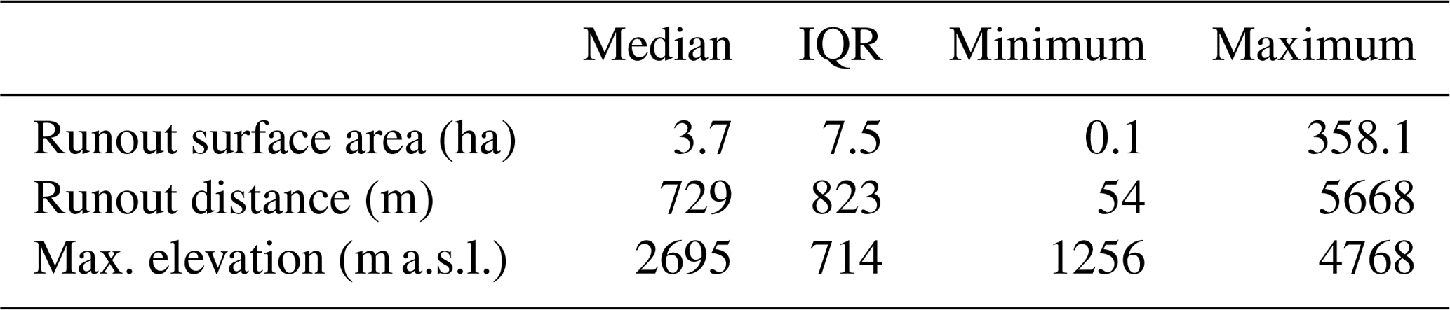
Note: IQR is the interquartile range.

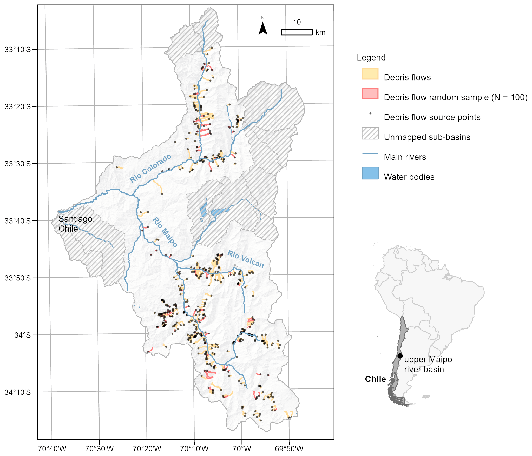
Figure 1 Map providing an overview of the debris-flow polygons and source points mapped in the upper Maipo River basin.

2.2 The debris-flow inventory

Debris-flow polygons and source points were mapped based on photointerpretation of high-spatial-resolution (0.50 m) satellite imagery (2000 to 2019) from CNES/Airbus and Maxar Technologies available through Google Earth Pro software, field observations, reviewed news articles and the compilation of data collected by public authorities. Each mapped polygon represents a debris-flow track that includes source, runout and deposition area. In total, 541 source points and 521 debris-flow polygons were mapped (Table 1). Manually mapping all debris flows across the upper Maipo basin is a challenging task due to its large geographical extent and its high abundance of mass movements. Therefore, a mapping strategy was employed that divided the basin into 58 sub-drainage basins (5439 km²), 45 (3936 km²) of which were selected for mapping (Fig. 1).

2.3 Modelling debris-flow source areas

Potential debris-flow source areas were spatially predicted using a generalized additive model (GAM). In general, GAMs demonstrate good performance for susceptibility modelling compared to other commonly used physically based and machine-learning techniques (Goetz et al., 2011, 2015b). To improve model generality and avoid overfitting, the GAM smoothing spline parameters were allowed a maximum five effective degrees of freedom (Wenger and Olden, 2012; Goetz et al., 2015a). The training and test data were based on the common 1:1 sampling strategy (Heckmann et al., 2014) of presence to absence of source points. The non-source (i.e. absence) points were randomly sampled within the mapped sub-basins outside of the mapped debris-flow polygons. The resulting training and test data contained 541 source points and 541 non-source points.

The predictor variables of source areas included hillslope angle, elevation, catchment area, plan curvature and distance to faults. These predictor variables generally have a high importance for modelling debris-flow initiation susceptibility as observed in previous works (Blahut et al., 2010b; Goetz et al., 2015b; Angillieri, 2020). The publicly available ALOS PALSAR radiometrically terrain corrected (RTC) high-resolution (12.5 m) digital elevation model (DEM; ASF DAAC, 2011) was used to derive terrain attributes. Before deriving the terrain attributes, mesh denoising was applied to the DEM to mitigate the propagation of artefacts such as high-frequency noise (Brock et al., 2020) in the prediction of source areas (Sun et al., 2007; Stevenson et al., 2010). We used the implementation of this algorithm in the System for Automated Geoscientific Analyses geographic information system (SAGA-GIS). After denoising, an algorithm to fill sinks (Planchon and Darboux, 2002) was applied to the DEM, and the terrain attributes were processed. Distance to faults was calculated as the Euclidean distance from the fault lines (Servicio Nacional de Geología y Minería de Chile 2003; scale 1:1 000 000).

The performance of the source-area prediction model was assessed using repeated k-fold spatial cross-validation (Brenning, 2012). Like cross-validation, spatial cross-validation randomly splits the data (e.g. source points and non-source points) into k disjoint subsets, where the model is trained using k−1 sets and tested with the remaining set during each cross-validation iteration. For spatial cross-validation, the data are divided into spatially disjoint sub-areas, in our case using the k-means clustering algorithm (Ruß and Brenning, 2010). This approach should provide a rigorous estimate of the spatial transferability of a model by attempting to reduce spatial autocorrelation between test and training data (Brenning, 2005; Wenger and Olden, 2012; Schratz et al., 2019). We estimated model performance by repeating 5-fold spatial cross-validation 1000 times. Model performance was measured using the AUROC, which is an overall measure of goodness of fit that is independent of any particular decision threshold.

2.4 Modelling debris-flow runout

The GPP (Wichmann, 2017) model was used to regionally model runout. The GPP model is an open-source framework in the SAGA-GIS software that provides users with various model components to simulate runout path, distance, velocity and deposition of material of mass movements (e.g. snow avalanches, rockfalls and debris flows). Due to the extent and remoteness of the study area, we focus on modelling the likely spatial patterns of runout. That is, we are not modelling flow velocity and depth.

Runout path was modelled using the random-walk process path component of the GPP model (Gamma, 2000). It is a common approach for debris-flow runout path modelling at medium scales (Mergili et al., 2012; Heckmann and Schwanghart, 2013; Mergili et al., 2015). Random-walk models the potential path of runout by iteratively simulating (via Monte Carlo simulation) the downslope movement of debris flows originating from source-area grid cells. These simulations result in a grid with runout frequencies that indicate how many times a grid cell is traversed: this is a cumulative frequency based on simulations from all source areas. There are three parameters that need to be calibrated to obtain a desired runout path: (1) a slope threshold (^∘) defining where divergent flow is allowed; (2) the exponent of divergence that controls the amount of divergence or lateral spreading in areas below the slope threshold; and (3) a persistence factor that controls the direction of movement (Wichmann, 2017). Flow path is determined using a 3×3 window that first controls the path of a central cell by considering only neighbouring cells with lower elevation. If the neighbouring cells are above the slope threshold, the neighbouring cell with the steepest descent is selected; otherwise, neighbours are assigned transition probabilities based on slope. These probabilities are adjusted using the exponent of divergence and the persistence factor. A higher exponent of divergence will result in more even probabilities across the neighbouring cells, allowing for a higher likelihood of not selecting the steepest descent path. The persistence factor considers the previous flow direction in weighting the probabilities. A higher persistence factor increases the probability that the selected neighbour will follow the direction of the previous cell. Based on these transition probabilities, a pseudo-random number generator selects a cell to define the flow path (see Wichmann, 2017, for a more detailed description). With this random-walk implementation, the flow path stops when the neighbouring cells have a higher or equal elevation compared to the central cell.

Runout distance was constrained using the two-parameter friction model (PCM; Perla et al., 1980) component of the GPP model. The PCM model, which is also a component of the Flow-R model (Horton et al., 2013), has also been used for modelling debris-flow behaviour at medium scales (Mergili et al., 2012; Heckmann and Schwanghart, 2013; Mergili et al., 2015). It is a centre-of-mass model where motion is mainly controlled by (1) the sliding friction coefficient μ and (2) the mass-to-drag ratio ($M/D$). In the GPP implementation of the PCM model, the velocity (m s⁻¹) at any grid cell v_i along a runout path can be characterized by the velocity of the previous grid cell v_i−1 (m s⁻¹), the local slope θ (^∘), distance between grid cells L_i (m), the acceleration due to gravity g (m s⁻²) and the friction parameters μ and $M/D$ (m):

$$\begin{array}{}\text{(1)}& v_i=\sqrt{{\mathit{\alpha }}_i\cdot (M/D)\cdot (\mathrm{1}-e^{{\mathit{\beta }}_i})+(v_{(i-\mathrm{1})}{)}^{\mathrm{2}}\cdot e^{{\mathit{\beta }}_i}\cdot \cos (\mathrm{\Delta }{\mathit{\theta }}_i)},\end{array}$$

where

$$\begin{array}{}\text{(2)}& {\displaystyle }{\mathit{\alpha }}_i=& {\displaystyle }g(\sin {\mathit{\theta }}_i-{\mathit{\mu }}_i\cos {\mathit{\theta }}_i),\text{(3)}& {\displaystyle }{\mathit{\beta }}_i=& {\displaystyle }{\displaystyle \frac{-\mathrm{2}{L}_i}{(M/D{)}_i}},\end{array}$$

and

$$\begin{array}{}\text{(4)}& {\displaystyle }\mathrm{\Delta }{\mathit{\theta }}_i=\left\{\begin{array}{lll}{\mathit{\theta }}_{\left(i-\mathrm{1}\right)}-{\mathit{\theta }}_i& & \text{if}{\mathit{\theta }}_{(i-\mathrm{1})}>{\mathit{\theta }}_i\\ \mathrm{0}& & \text{if}{\mathit{\theta }}_{(i-\mathrm{1})}\le {\mathit{\theta }}_i\end{array}\right\}.\end{array}$$

For the case of a concave transition in the slope direction between grid cells, a velocity correction (Eq. 4) based on the conservation of linear momentum is applied (Wichmann, 2017). The μ controls the velocity of movement through the runout path and $M/D$ controls velocity movement over steep terrain. The conditions for acceleration along the runout path can be described by

$$\begin{array}{}\text{(5)}& \tan {\mathit{\theta }}_i>{\mathit{\mu }}_i,\end{array}$$

and deceleration by

$$\begin{array}{}\text{(6)}& \tan {\mathit{\theta }}_i<{\mathit{\mu }}_i.\end{array}$$

We can use Eq. (6) to help interpret μ, as it can be used to characterize the slope angle under which deposition begins and termination of runout occurs (Perla et al., 1980).

2.4.1 Optimizing model parameters

For regionally applying the runout model, we needed to determine the combination of model parameters that result in the best match to our debris-flow inventory. Determining optimal parameters was based on two criteria: (1) the ability of the model to capture our observed runout paths and (2) its ability to match the observed runout distances. Therefore, we performed this optimization task using a two-stage approach that first optimizes the random-walk model and then the PCM model parameters.

A random sample of 100 debris-flow tracks and corresponding source points was used for optimizing the runout models. This sample of the inventory was chosen to facilitate quality control and reduce the computational complexity of the optimization. Source areas were determined by buffering each source point by 50 m and masking away the buffered area that exceeds the runout trimline; this ensures the source area is contained within a mapped debris-flow polygon. A sink-filled version of the original DEM was used for the runout modelling.

For each model component, an exhaustive grid search in parameter space was used to find parameter sets that achieve optimal model performance across all sampled debris flows. The search ranges were similar to Wichmann's (2017) suggested parameter limits for debris flows (see Table 2 for value ranges). We additionally tested the use of a spatially varying sliding friction coefficient. The value for this spatially varying sliding friction coefficient μ_i was calculated as a function of catchment area a (km²) for maximum runout (Gamma, 2000; Wichmann and Becht, 2006; Mergili et al., 2012; Wichmann, 2017):

$$\begin{array}{}\text{(7)}& {\mathit{\mu }}_i=\mathrm{0.13}{a}^{-\mathrm{0.25}}.\end{array}$$

Similar to Mergili et al. (2012) and suggested by Wichmann (2017), the spatially varying μ_i was set to a maximum of 0.3 and minimum of 0.045. Runout was computed using 1000 model iterations.

Table 2 Runout model grid-search optimization setup and results. Optimization performance was assessed using spatial cross-validation (CV).

Note: IQR is the interquartile range; a is the catchment area (km²).

The AUROC was used as a performance measure for the random-walk model. The receiver-operating characteristic (ROC) is a plot of the true positive rate versus the false positive rate. AUROC values range from 0.5 (random discrimination between classes) to 1.0 (a perfect classifier; Zweig and Campbell, 1993). Model performance was rated higher if the random-walk model contained observed debris-flow tracks within its simulated paths. After optimizing the random-walk model, we fixed these parameters for the PCM model and optimized the μ and $M/D$ parameters for determining runout distance. The performance of the PCM model was measured using the relative error of runout distance. Relative error was used so that each debris flow was weighted equally regardless of its magnitude. The AUROC was used to break any ties in relative error performance between multiple optimal parameter sets.

Runout distance was measured in terms of horizontal length of the debris-flow track. This distance was measured as the length of a minimum area bounding box containing the observed debris-flow track (Fig. 2; Niculiţa, 2016; Taylor et al., 2018). Estimated debris-flow tracks were defined as grid cells with values greater than a median runout frequency (Fig. 2). In this case, the median value represents the most typical simulated debris-flow track. It also provides a conservative estimate of runout distance, which helps mitigate the chance that the optimized model regionally underestimates runout distances.

Figure 2 Illustration of runout-distance optimization of the sliding friction coefficient μ using a minimum-area bounding box as a measure of travel distance – $M/D$ fixed at 40 m.

In addition to determining a global optimal parameter set, the best-performing parameters for individual debris-flow events were also explored. We similarly applied a grid search to each event and determined optimal parameter sets based on the performance (AUROC and relative error) of each runout model component.

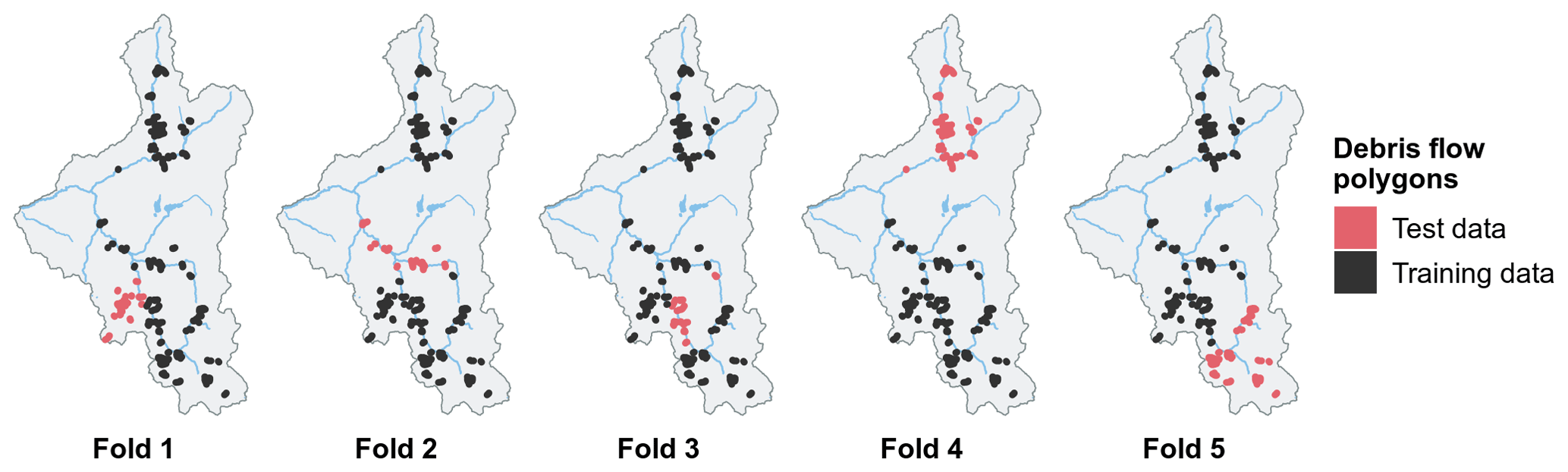
Figure 3 An example realization of random partitions based on k-means clustering of debris-flow polygons for a single repetition of 5-fold spatial cross-validation. The selection of these debris-flow polygons was based on a random sample.

2.4.2 Assessing spatial transferability

Based on our random sample of 100 debris-flow tracks, we assessed the transferability of optimized runout model (random-walk and PCM) parameters by performing 5-fold spatial cross-validation with 1000 repetitions (Fig. 3). This approach allows us to explore the sensitivity of grid-search optimized parameter combinations to spatial variation in training and test data. To do this, we observed the frequency of variations in optimized parameter combinations within all cross-validated iterations. Optimal parameter combinations that occurred more frequently were considered to have a higher degree of transferability, thus being considered more reliable for application to the entire study area.

We also assessed if there were any spatial patterns in the optimized performance for each model component. That is, were there any spatial trends in model performance that may indicate our model is locally overfitting? We explored such spatial trends by mapping the distribution of individual debris-flow runout model performance based on the optimized parameters. Additionally, we were concerned if the optimized parameters had a stronger fit to debris flows of a certain magnitude or initiating conditions. Therefore, the potential to overfit to certain debris-flow characteristics was assessed by determining Spearman's rank correlation (ρ) of individual debris-flow performance (for each model component) with observed runout distance and the elevation, catchment area and hillslope angle of the corresponding source points.

2.4.3 Testing sample-size dependence of performance

We explored how runout model parameter selection, performance and robustness were affected by the number of debris flows used for optimization. Spatial cross-validation was applied to data sets of varying training sample sizes using the random sample of 100 debris flows used for model optimization. To ensure a fair comparison, the size of the test data for each cross-validation iteration was set to 20 debris flows, which is the maximum test sample size when performing 5-fold spatial cross-validation with a sample of 100 debris flows. We tested training samples sizes from 10 to 80. Model performance for each runout modelling component was summarized using the median and interquartile range (IQR) (AUROC and relative error). The optimal parameter sets for a given sample size were determined as the parameter combinations that were most frequent.

2.4.4 Finding a suitable source-area prediction threshold

For regionally applying the runout model for susceptibility mapping or exposure analysis, a dichotomous classification of the predicted source areas is required to define the grid cells where simulated debris flows initiate. In the case of basing the source areas on a susceptibility model, a suitable threshold of the prediction values needs to be selected. In this study, we determine a suitable prediction threshold to classify source areas by searching for the threshold that results in the best-performing runout model for the entire area. Using the optimized model parameters, we tested runout models based on source areas that were delineated using prediction thresholds from 0.5 to 0.95 with a step of 0.05. The performance of each these models was measured using the AUROC. The AUROC was calculated using a sample of 1000 debris-flow runout locations and 1000 locations outside of the debris-flow polygons. The source-area prediction threshold resulting in the highest AUROC values was selected for regionally computing a debris-flow runout map for our study area.

2.5 Geocomputing and visualization software

The methods for runout modelling optimization, validation and visualization of the source-area prediction and runout modelling were implemented using the open-source statistical software R (ver. 3.6.2; R Core Team, 2019) and SAGA GIS (version 6.1; Conrad et al., 2015) with its GPP model tool (Wichmann, 2017). Coupling SAGA GIS with R was done using a combination of the RSAGA (Brenning et al., 2018) and Rsagacmd (Pawley, 2019) packages. The GAM was implemented using the mgcv package (Wood, 2011). General handling of spatial data in R used the sf (Pebesma, 2018), sp (Pebesma and Bivand, 2005), rgeos (Bivand and Rundel, 2019), rgdal (Bivand et al., 2019) and raster (Hijmans, 2020) packages; spatial cross-validation was applied using the sperrorest (Brenning, 2012) and ROCR (Sing et al., 2005) packages. Parallelization of the optimization and validation procedure used foreach (Microsoft and Weston, 2020). Visualization was done using R's ggplot2 (Wickham, 2009) and metR (Campitelli, 2020) packages and ESRI's ArcMap (ver. 10.5).

3 Results

3.1 Source-area model performance

The overall performance of the source-area prediction based on the GAM was good with a spatially cross-validated median AUROC of 0.80 and an IQR of 0.001. We found the source-area prediction map was also geomorphologically plausible. Locations most likely to be source areas were within steep terrain associated with channels, gullies and scree slopes. Shallow-flat terrain and areas along ridgelines were modelled as least likely to be source areas (Fig. 4). This geomorphological knowledge was also expressed in the plots of the GAM spline transformations (Fig. 5). Relatively steep terrain, slightly concave plan curvature and areas near faults were modelled as more likely being source areas.

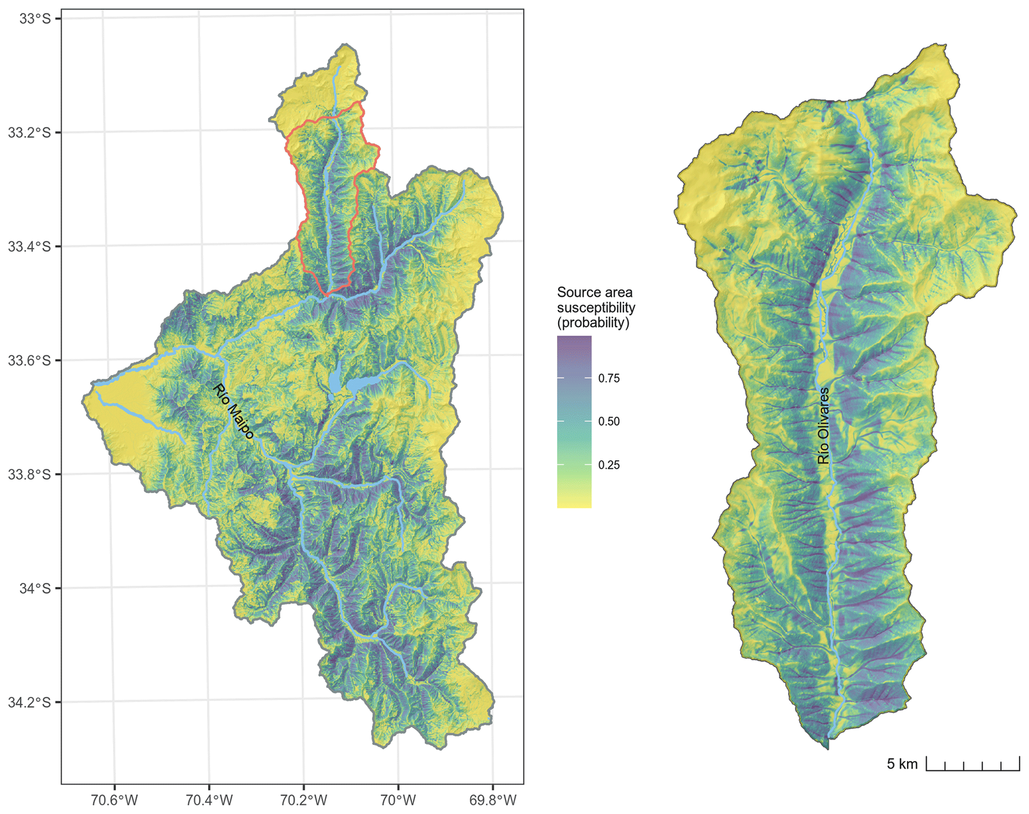
Figure 4 Map of the debris-flow source-area prediction based on a GAM.

Figure 5 Transformation of predictor variables in the generalized additive model, where the y axis can be interpreted as the associated likelihood (log odds) of being a source area. Terms of the form s(predictor) indicate a nonlinear smoothing spline transformation. The effective degrees of freedom (EDFs) refer to the flexibility of the smoothers. The dashed lines represent confidence bands at a 95 % level.

3.2 Runout model parameter optimization

The parameter optimization produced runout models with a good spatially cross-validated performance. The optimal parameters for the runout-path model were a slope threshold of 40^∘, an exponent of divergence of 3.0 and a persistence factor of 1.9 with a median AUROC of 0.94 (IQR=0.02; Table 2). Using these values as plug-in estimates for the PCM runout-distance model component, the optimal μ and $M/D$ were 0.11 and 40 m, respectively. The median spatially cross-validated relative length error of the runout-distance model was 0.11 or 11 % (IQR=0.09). We also found that the model based on a global μ estimate performed better than the runout-distance model using the spatially varying μ_i (optimal $M/D=\mathrm{95}$ m; Table 2), which had a median relative error of 0.19 (IQR 0.09).

By visualizing the runout-distance optimization results across grid search space, we can observe model performance and sensitivity to different parameter combinations. In this case, we observed only slight model performance differences for μ values just under 0.2 to 0.04 and $M/D$ values from 20 to 150 m (Fig. 6a). In general, the values in this band across grid search space would result in good performance with median relative errors ≤0.15. However, in terms of controlling the spread of error (Fig. 6b), μ values from about 0.05 to 0.15 and $M/D$ values from 20 to 95 m had the lowest IQRs (≤0.2).

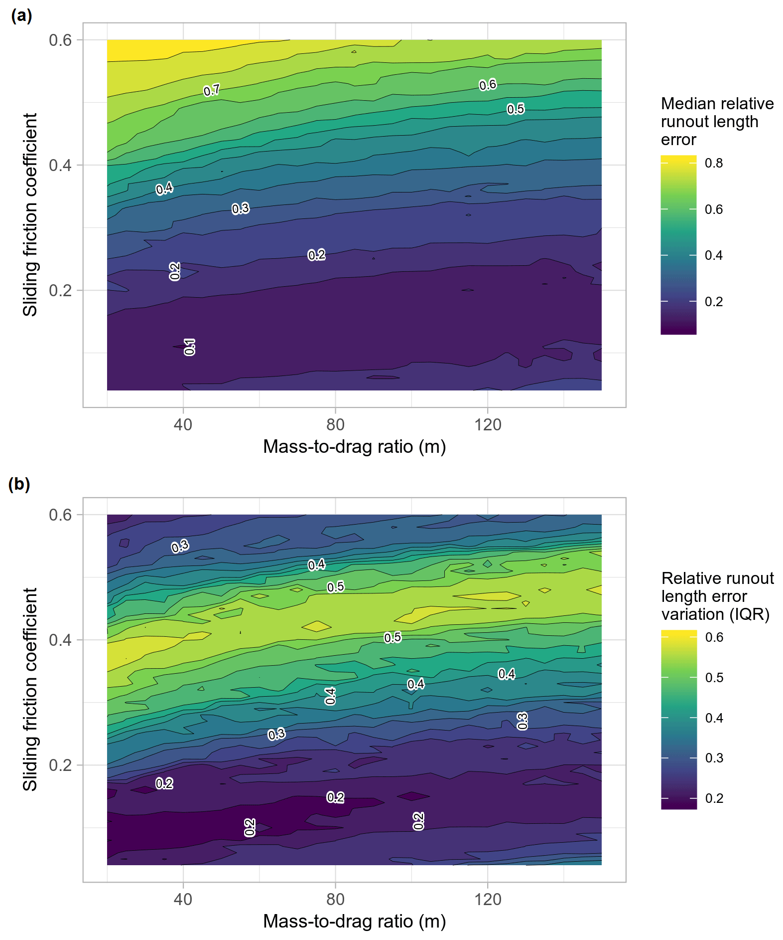
Figure 6 Density contour plots of parameter optimization of sliding friction coefficient μ and $M/D$ in the PCM model, illustrating median relative runout length errors (a) and the associated variations in relative error (b) using the IQR.

Exploring the optimal combination of parameter values using spatial cross-validation provides insights into performance reliability of the optimized model. Given different spatial combinations of testing and training data, we found that the optimal combinations of parameters were associated with high performance values (AUROC=0.94, relative error=0.11) and high relative frequencies (61 %–69 %) of occurring in each cross-validation iteration (Fig. 7). Additionally, the spatial-cross-validated optimal parameter sets were generally clustered in grid search space, showing there was little variation in optimized parameters depending on the spatial partitions (Fig. 7). In terms of obtaining multiple optimal solutions, only 5 % of the total 5000 cross-validation iterations had ties in relative error performance.

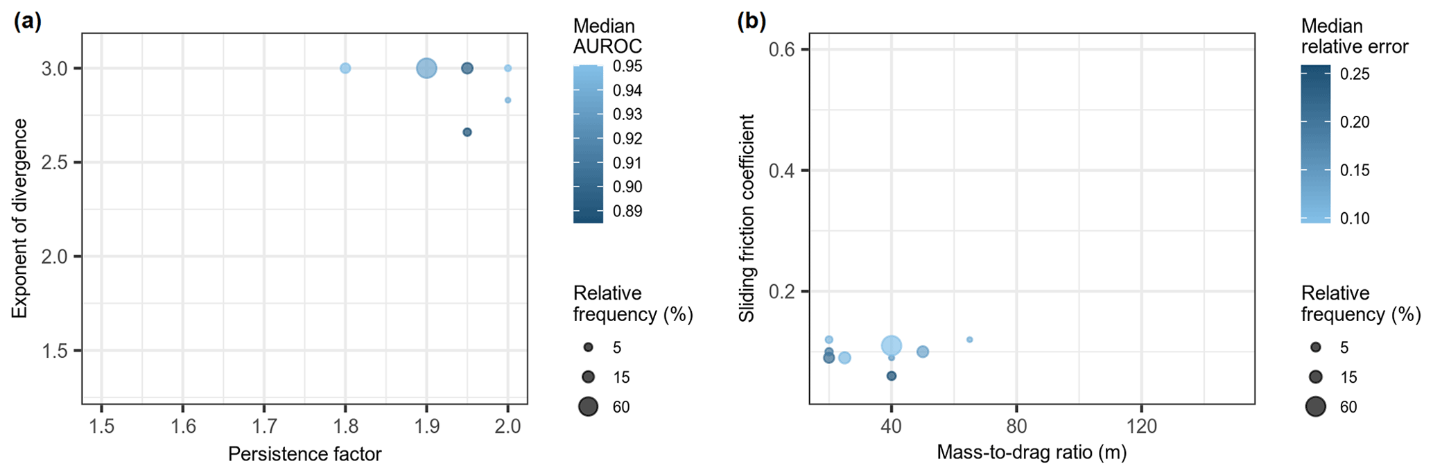
Figure 7 Model performance and frequency of optimal parameters for the runout path (a; given an optimized slope threshold of 40) and runout-distance models (b) estimated using 1000 repetitions of 5-fold spatial cross-validation. Relative frequency is the percentage of all repeated spatial-cross-validation iterations where a given parameter combination was optimal.

3.3 Thresholding source areas for runout analysis

The best threshold for delineating source areas from the GAM prediction for runout modelling was 0.7, which results in runout affecting 22 % of the study area. This threshold had the peak AUROC value of 0.83. The performance of the runout model drastically decreased with thresholds >0.8 and gradually decreased towards a threshold of 0.5: lower thresholds spatially predicted more runout area (Fig. 8). The runout prediction map resulting from the best threshold (Fig. 9) appears to be geomorphologically plausible. The locations of the runout deposit areas are similar to what we have observed in the satellite imagery. Additionally, lateral spreading is generally low in narrow gullies and much broader on talus slopes, which is what we would expect for debris flows occurring in our study area.

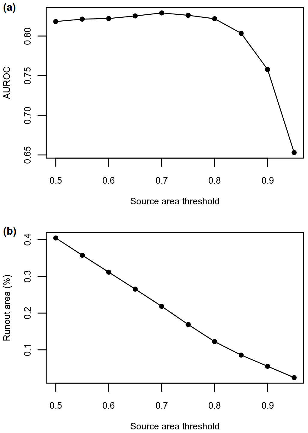
Figure 8 Performance of debris-flow runout model for different source-area thresholds (a) and percentage of study area impacted by runout (b). Optimal threshold was a threshold of 0.70 (AUROC = 0.83) with runout affecting 22 % of the study area.

Figure 9 Map of optimized debris-flow runout model based on global parameters and source-area threshold of 0.70.

3.4 Exploring patterns in model performance

We observed no clear spatial pattern of individual debris-flow performance of the runout model components (Fig. 10), which is evidence that there was no local overfitting to a particular region of the study area. The distribution of individual AUROC performance of the runout path model was generally high for most of the region, showing that optimization of the path model performs well across the study area. One debris flow was not captured within the runout path model (AUROC<0.5; Figs. 10 and 11). Having a closer look at this occurrence, we found that the modelled runout paths failed to follow the flow direction of the observed debris flow and source point.

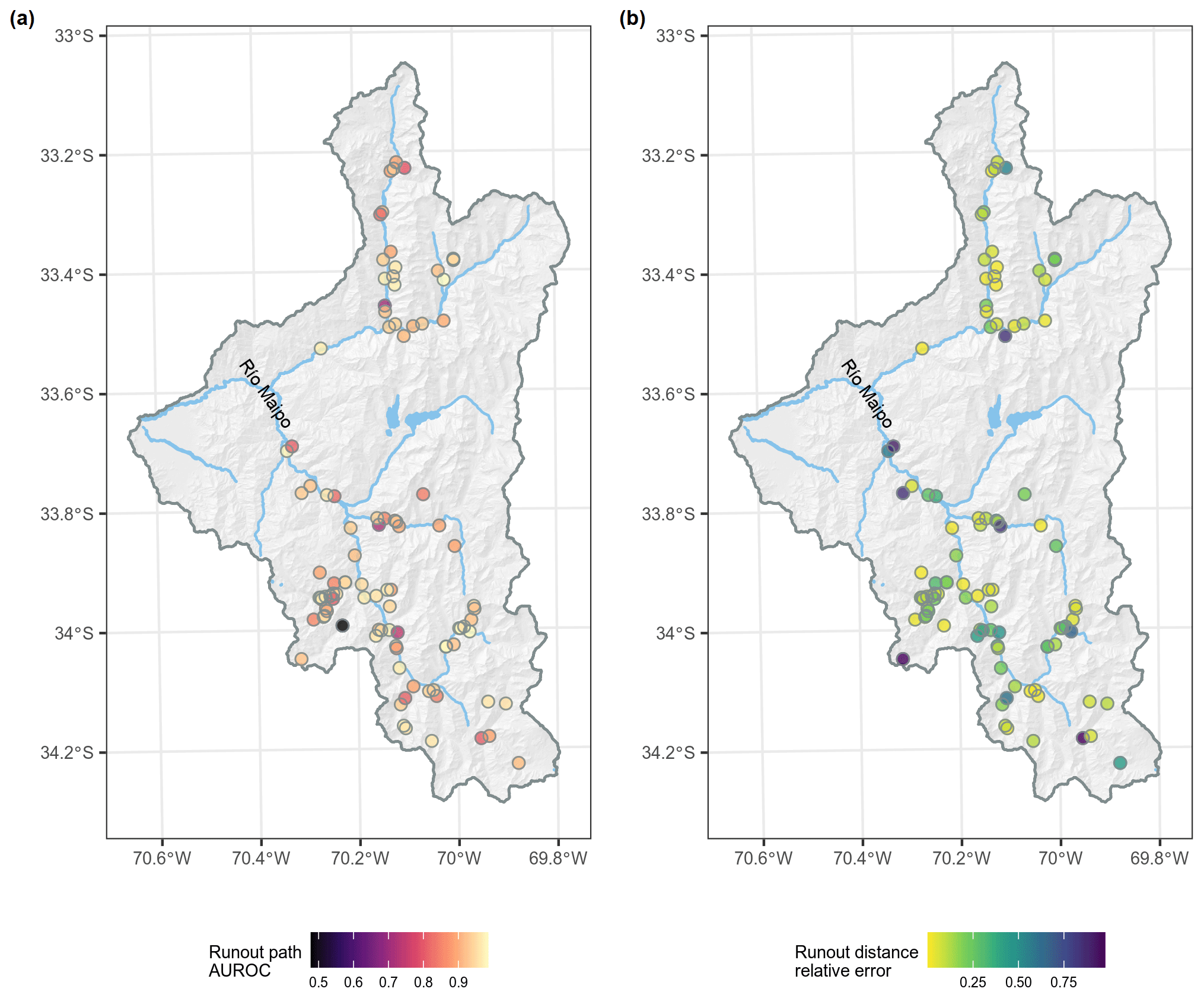
Figure 10 Maps of the performance of the runout path (a) and runout-distance models (b) for individual debris flows based on the global optimal parameters.

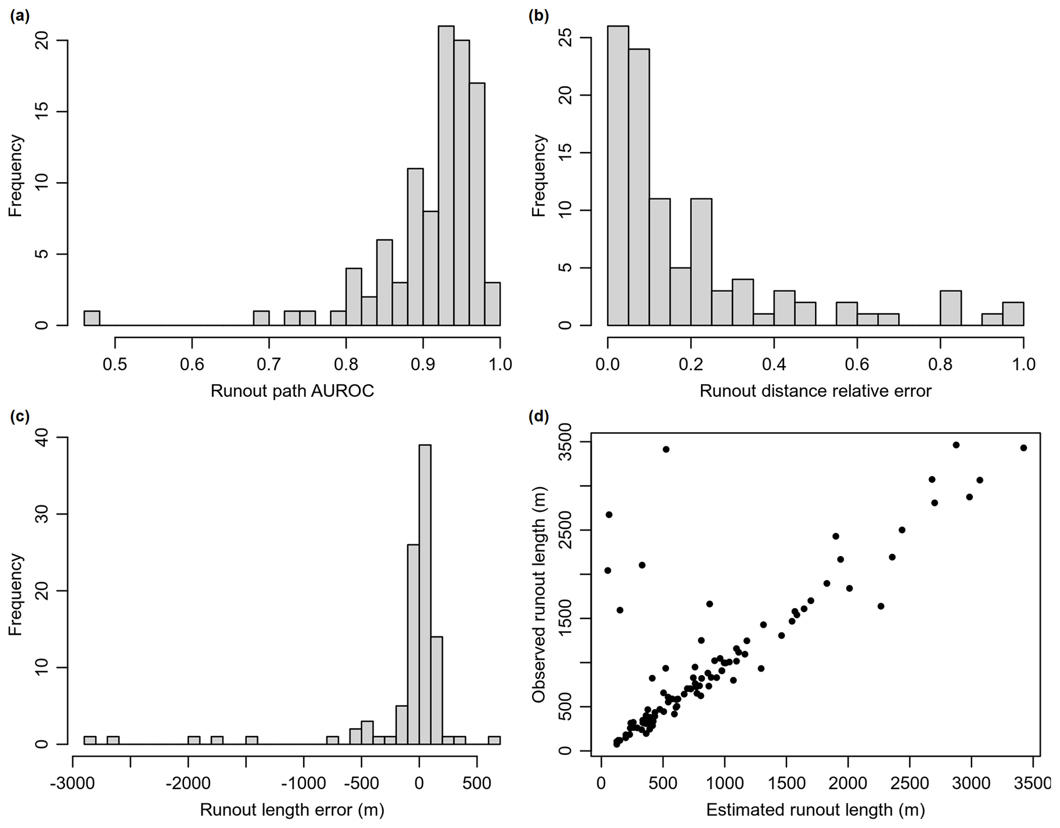
Figure 11 Histogram of performance of the runout path (a), runout-distance models based on relative error (b), actual runout length error (c) and a plot of observed runout lengths versus modelled runout lengths (d).

The runout-distance model had generally more spatial heterogeneity in performance (Fig. 10), but again no clear spatial patterns in the distribution of relative errors were observed. We investigated the debris flows that did not perform well for modelling runout distance (relative error >0.8) by looking at the satellite imagery used for mapping and the DEM derived hillslope angle. It was found that these cases were related to misclassifying stream erosion in relatively shallow and long-hillslope channels as debris flows.

Overall, the regionally optimized runout modelled distances fit well with our mapped observations (Fig. 11). It tended to slightly overestimate debris-flow travel lengths with a median runout-distance error of 16.6 m (Fig. 11). This error is just slightly over a single grid cell size of the DEM. The highest runout-distance errors were due to misclassified debris flows, as previously mentioned. The optimization of the runout model avoided overfitting to debris-flow tracks of a certain magnitude and general terrain conditions. That is, we did not observe a strong correlation between runout-distance performance to length of observed debris flow ($\mathit{\rho }=-\mathrm{0.36}$), starting elevations (−0.21), catchment area (0.11) or hillslope angle (0.29) of source points used for model training.

3.5 Optimization for individual debris flows

The optimal parameters for individual debris flows were also computed for general comparison to the regional model. We found that the optimized runout model parameters were highly variable for individual debris flows (Fig. 12). The relative errors were low (median=0.002, IQR=0.007), except for a few debris flows that failed to optimize (Fig. 11). Multiple optimal solutions for the PCM model occurred in 56 % of the events. However, after tie breaking using the AUROC, the number of multiple optimal solutions was down to 3 %.

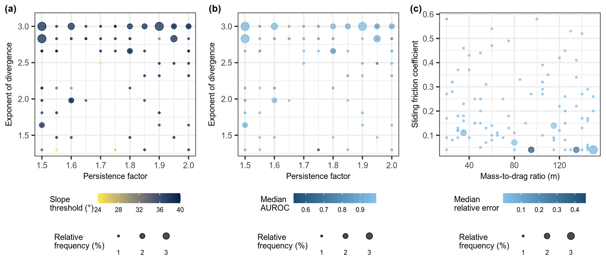
Figure 12 Performance and frequency of runout path (a, b) and distance (c) optimal parameters determined for individual debris flows. Relative frequency is the percentage of all repeated spatial-cross-validation iterations where a given parameter combination was optimal.

Most individual events optimized runout paths with parameter sets leading to high lateral spreading. The optimal-path parameters for most of the individual events had a 40^∘ slope threshold, high exponent of divergence and low persistence values (Fig. 12a). By individually examining the optimal simulated paths for each training event, we observed that ∼60 % of the observed debris-flow tracks did occur within the most frequent simulated paths. The other events were typically located on the fringes of the most frequent paths.

There was no clear spatial pattern in optimal μ and $M/D$ parameter combinations across the study area, which shows that runout characteristics were quite diverse for individual debris flows across this large study area (Fig. 13). We also observed no strong relationships between terrain attributes and optimal parameters. Spearman's correlations of μ and $M/D$ with elevation, slope and catchment area were $\le \left|\mathrm{0.29}\right|$.

Figure 13 Map of runout-distance model optimal parameters determined for individual debris flows.

3.6 Runout model robustness to sample size

Runout model performance and variation tends to improve slightly when using larger sample sizes (Fig. 14). Large sample sizes also resulted in more consistently selected model parameters across spatial-cross-validation iterations (Fig. 15). The larger spread across grid search space of the relative frequency of optimal parameter combinations for smaller sample sizes illustrates that we may be less likely to find the best model parameters that generalize well for a large region (Fig. 15). In general, as we increased sample size, we reduced sampling variability and narrowed the number of optimal combinations of parameters in grid search space, meaning we became more confident that the selected parameters would transfer better to estimate runout distance in adjacent areas.

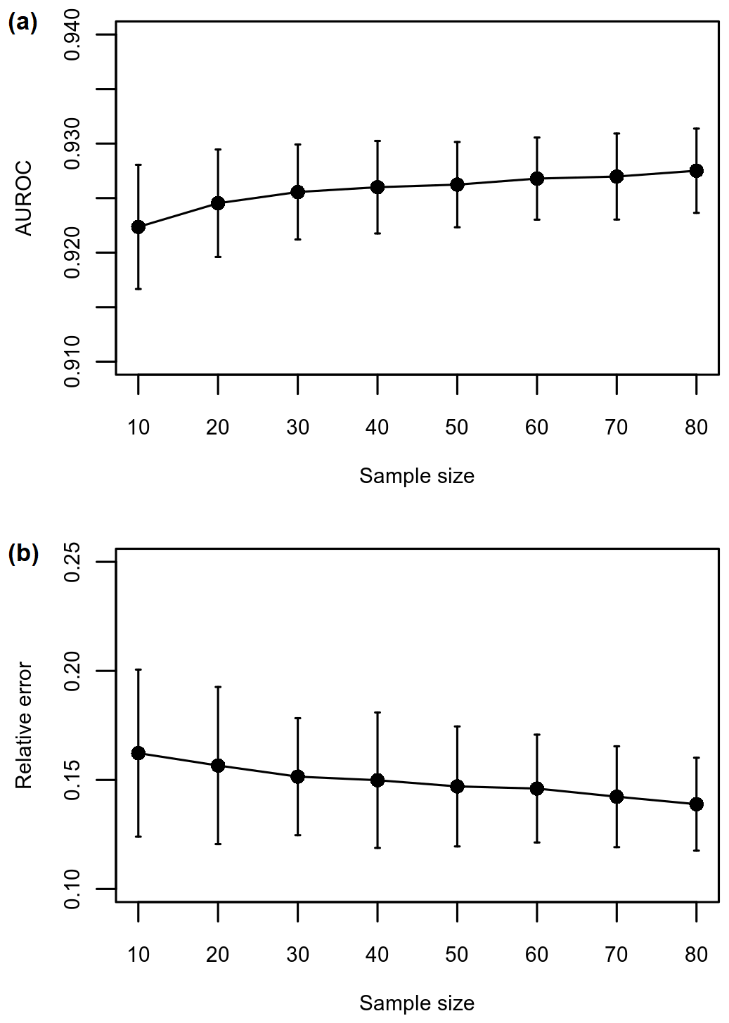
Figure 14 Comparison of runout path (a) and distance (b) performance for different model training samples sizes assessed using spatial cross-validation. The error bars indicate the standard deviation in performance.

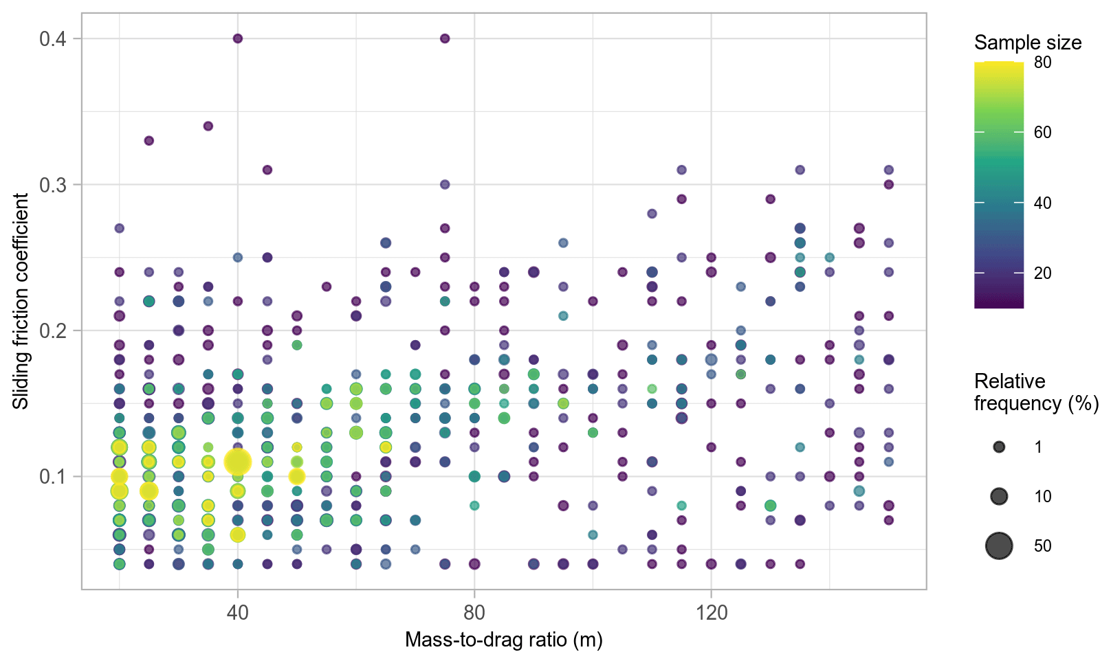
Figure 15 Relative frequencies of optimal parameter combinations for different training sample sizes computed using spatial cross-validation.

4 Discussion

4.1 Model performance and transferability

Assessing the spatial transferability of runout models is essential when extending their use from single or local events to regionally modelling runout across unknown space. Overall, this study demonstrates that our novel optimization approach performed well at regionally modelling the spatial distribution of runout path and distances across the upper Maipo River valley basin. A key component of the success of our modelling approach was its ability to generalize. The transferability of a regional runout model can be affected by the generalization ability of both the source-area prediction and the optimized process-based runout model.

4.1.1 Source-area modelling

In the development of our source-area prediction model, we aimed to produce a simplified empirical model that would result in good performance and transferability. Wenger and Olden (2012) recommended to control the flexibility of the GAM smoothing parameters to avoid overfitting that would lead to poorer model transferability. Therefore, similarly to previous landslide susceptibility studies using the GAM (Goetz et al., 2011, 2015a; Bordoni et al., 2020), we limited the degrees of freedom for smoothing-spline fitting.

A detailed model based on a large set of predictors can impede its ability to transfer to other locations (Tuanmu et al., 2011). As we and others have demonstrated, good predictive performance of susceptibility models of debris flows can be achieved with a relatively small set of predictors, which are primarily DEM-derived terrain attributes (Blahut et al., 2010b; Heckmann et al., 2014; Goetz et al., 2015b). Additionally, by fitting our models with multi-temporal data, we may be more likely to achieve better transferability in time (Tuanmu et al., 2011; Knevels et al., 2020). Event-specific inventories may not be large enough for regional optimization and risk the potential of overfitting source conditions to spatially varying conditions of that event (e.g. precipitation and snowmelt patterns). A smaller sample may also lead to not capturing the range of terrain conditions across the study area required for robust empirical modelling of source-area locations (Petschko et al., 2014; Rudy et al., 2016).

The interpretability of the GAM allows us to explore modelled behaviour. For our study, the GAM did well at representing the general geomorphic characteristics of source areas. Some of the relationships between predictors, such as elevation, and debris-flow activity can be complex. In the upper Maipo River basin, elevation can be a proxy for vegetation, snow cover duration, terrain ruggedness, permafrost and glacial bodies, and geology. It is therefore difficult to discern any direct relationships between elevation and likelihood of being debris source areas. However, we suspect that lower elevations were predicted to be less prone to be source areas due to increased vegetation cover and less rugged terrain. The decrease observed at the highest elevations may relate to permafrost and glacial bodies holding potentially mobilized sediment (e.g. Sattler et al., 2011). A decrease in predicted likelihood of source areas occurring at high slope angles ($\sim >\mathrm{45}{}^{\circ }$) may be associated with steep rock faces that were more likely sources of rockfalls than debris flows (Loye et al., 2009).

4.1.2 Runout analysis

The best-performing regional random-walk parameters allowed for maximum lateral spreading of the runout path given the range of parameters for optimization. Individual events tended to also optimize for high lateral spreading but not as strongly as the regional model. We believe this high lateral spreading may be due to the location of the observed debris flows relative to simulated paths and the quality of the DEM. A large proportion of the observed debris-flow tracks were located at the fringe of the most frequent simulated paths. Thus, a higher slope threshold and exponent of divergence are required to capture these fringe debris flows. Additionally, the surface of DEMs with resolutions greater than 20 m can be too general to capture minor gullies that may have high flow accumulation (Blahut et al., 2010b). The 12.5 m resolution ALOS DEM used in this study is derived from downsampled Shuttle Radar Topography Mission (SRTM) data and would likely contain some of the topographic generalizations of the original DEM (∼30 m spatial resolution). Despite potential issues with DEM quality, similarly to Horton et al. (2013), we illustrated valuable results can still be achieved.

By optimizing the runout-distance model using the median relative error as a metric, we managed to reduce the impact of possible outliers in our training and test data. We additionally reduced our chances of overfitting the regional model to larger debris-flow events, which was crucial for a model to maintain a generalization that makes it transferable across large areas.

Plotting the individual optimized models and exploring correlations between terrain attributes and optimal parameters allowed us to see if there were any broad trends in the parameter selection. In our study, we observed high variability in optimal parameters of the PCM model. While applying a trial-and-error approach, Mergili et al. (2012) also observed different optimal parameter combinations for individual events when modelling runout for a couple of debris flows just north of our study area. It seems apparent that determining runout parameter values for regional modelling without an optimization procedure would be difficult. It is also no surprise that the errors of the individually optimized debris flows were low (Fig. 12). Whether meaningful or not, the optimization approach should be able to match the runout distance with very low error. Poorly individually optimized events could be attributed to locally poor DEM quality (Horton et al., 2013) and mapping uncertainties (Ardizzone et al., 2002).

The two-parameter PCM model has a uniqueness problem (Perla et al., 1980). Possibly infinitely many pairs of μ and $M/D$ can result in the same runout distances. When optimizing individual events, we did observe this phenomenon. The majority of individual events had more than one optimal combination of parameters. Obtaining a unique solution was not an issue for the regional optimization in our study for the given grid search space. Likely this is due to having to satisfy the runout distances for a variety of hillslope conditions and lengths across the study area. The observed reduced variability in optimal solutions for larger sample sizes (Fig. 15) provides some evidence for this conjecture.

Although we obtained a unique regional model solution, runout-distance relative errors were only slightly higher than the best performer for combinations of μ and $M/D$ across a band in grid-search space of lower μ values (Fig. 6). We believe this model performance insensitivity to μ is due to decrease in slope being one of the main factors controlling runout distance. The lowest relative errors tended to occur when the slope condition for deceleration was in the range of 2.3 to 11.3^∘, and the optimal was 6^∘ (μ>0.04, μ>0.20 and μ>0.11; Eq. 6; Fig. 6). This range matches well to the slope values observed at or near the stopping locations of the debris flows used to train the PCM model. These results are also very similar to modelled observations of debris-flow runout in the semi-arid Andes by Mergili et al. (2012). They observed that best PCM runout modelling results for individual events occurred when deposition began at slope angles ranging from 2.6 to 14.0^∘ (μ>0.045 and μ>0.25). Additionally, this range fits within other global observations of debris-flow deposition occurring on slopes smaller than 6 to 17^∘ (Hungr et al., 1984; Ikeya, 1989; Rickenmann and Zimmermann, 1993; Bathurst et al., 1997; Lorente et al., 2003). The insensitivity across $M/D$ values (Fig. 6) is due to many possible solutions for obtaining similar runout distances with different combinations of μ and $M/D$ (i.e. the uniqueness problem). The range of μ values resulting in low relative error only slightly increased with higher $M/D$ value, which indicates that μ had a much stronger role than $M/D$ in governing runout distances.

In theory, it is possible that the minimum area-bounding box could contribute to parameter insensitivity. Abrupt changes in flow perpendicular to the initial flow direction, such as a flow meeting a channel, may only slightly increase the length of the bounding box for several iterations of decreasing μ (or increasing $M/D$). However, we did not observe this to be an issue within our training data for our given parameter ranges of μ and $M/D$.

4.2 Regionally optimizing runout models

As with any optimization problem, using a suitable cost function is critical to ensure the model parameters are optimized to solve a very specific problem. It can be difficult to define a single metric that simultaneously measures both performance of path and distance simulations. As shown in this study, it may also not be necessary. The modular framework of the GPP model provides the ability to optimize two distinct runout components, the runout path including lateral spreading and the runout distance. In our study, we used the random-walk and PCM components of the GPP model to simulate spatial extent of runout. By using the two-stage approach to optimization, where we first optimize the runout path model and then plug in those values to optimize the runout-distance model component, we can considerably reduce computational complexity, while ensuring that our final model result explicitly optimizes for runout distance – a key characteristic for spatially predicting areas potentially impacted by debris-flow runout. In our case, we only needed to solve two separate problems with three (random-walk) and two (PCM) unknown parameters, as opposed to solving simultaneously for five unknowns. We used an exhaustive grid search to optimize the runout model components because it allowed us to visualize and assess model performance across parameter space. However, a drawback of this optimization method is that it can be computationally slow to explore all candidate parameter combinations. If speed is a requirement for regional runout analysis, then a faster method like random search (Bergstra and Bengio, 2012) may be preferred (Schratz et al., 2019).

In terms of model improvement, analysis of the spatial distribution of optimal parameters may lead to better parameter optimization based on terrain or geological characteristics. The spatially varying values used in this study were based on modelling for alpine regions (Gamma, 2000) and do not account for the potential variability in sliding conditions between different catchments (Guthrie, 2002). This challenge may be overcome by using regional modelling strategies already applied for landslide initiation susceptibility modelling, where the study area is divided into geologically similar regions, runout model optimization is performed for each region and then combined (e.g. Petschko et al., 2014).

5 Conclusions

Modelling the spatial pattern of debris-flow runout in large, mainly remote areas, with sparse data, requires model calibration and validation methods that ensure spatial transferability. In this study, we demonstrated that the combination of the statistical prediction (GAM) of source areas and our regional optimization of the GPP runout model (random walk and PCM) performed well at generalizing runout patterns across the upper Maipo River basin. In addition to high model performance, the transparency and interpretability of the GAM provided further confidence in the prediction of source areas by illustrating regionally geomorphically plausible modelled behaviour. The optimized runout model parameters sets were consistently similar within grid search space when assessing transferability using spatial cross-validation. We believe this strong transferability of our runout model was due to the hillslope gradient of the deposition area being one of the major controls of runout distance in the PCM model. The regionally optimized runout model also resulted in geomorphically plausible results, with best-performing μ and $M/D$ combinations occurring when simulated debris-flow deposition and termination occurred on slopes less than 11^∘. Although obtaining unique PCM parameter solutions for individual events can be an issue, we were able to obtain a unique PCM model solution for our regional model. In general, we found unique regional-optimal PCM model solutions were more prone with larger sample sizes, as well as higher model performance and lower uncertainties. Future improvements to our approach may include building a model that allows for more spatial variation in optimized parameters, especially in regions with better availability of soil physical information. Overall, our open-source modelling approach, which enhanced the GPP model by adding support for automated model calibration and transferability assessment, provides an accessible and extendible modelling framework for such advances in regional runout modelling.