the Creative Commons Attribution 4.0 License.
the Creative Commons Attribution 4.0 License.
 | 25 Jan 2021
Trivariate copula to design coastal structures
Olivier Orcel
Philippe Sergent
François Ropert
Some coastal structures must be redesigned in the future due to rising sea levels caused by climate change. The design of structures subjected to the actions of waves requires an accurate estimate of the long return period of such parameters as wave height, wave period, storm surge and more specifically their joint exceedance probabilities. The simplified Defra method that is currently used in particular for European coastal structures makes it possible to directly connect the joint exceedance probabilities to the product of the univariate probabilities by means of a single factor. These schematic correlations do not, however, represent all the complexity of the reality because of the use of this single factor. That may lead to damaging errors in coastal structure design. The aim of this paper is therefore to remedy the lack of robustness of these current approaches. To this end, we use copula theory with a copula function that aggregates joint distribution functions to their univariate margins. We select a bivariate copula that is adapted to our application by the likelihood method. In order to integrate extreme events, we also resort to the notion of tail dependence. The optimal copula parameter is estimated through the analysis of the tail dependence coefficient, the likelihood method and the mean error. The most robust copulas for our practical case with applications in Saint-Malo and Le Havre (in northern France) are the Clayton copula and the survival Gumbel copula. The originality of this paper is the creation of a new and robust trivariate copula with an analysis of the sensitivity to the method of construction and to the choice of the copula. Firstly, we select the best fitting of the bivariate copula with its parameter for the two most correlated univariate margins. Secondly, we build a trivariate function. For this purpose, we aggregate the bivariate function with the remaining univariate margin with its parameter. We show that this trivariate function satisfies the mathematical properties of the copula. We finally represent joint trivariate exceedance probabilities for a return period of 10, 100 and 1000 years. We finally conclude that the choice of the bivariate copula is more important for the accuracy of the trivariate copula than its own construction.
- Article
(1902 KB) - Full-text XML
- BibTeX
- EndNote


The design of coastal structures requires the multiplicity of variables and their degree of correlation to be taken into account. We must therefore address the lack of robustness in the modelling procedure of the dependencies between the different variables characterizing the sea state (Sergent et al., 2014; Hawkes, 2005) such as wave height H, wave period T and storm surge S. The design of coastal structures is based in particular on the return periods of wave overtopping or of armour damage (Ciria et al., 2007). Since the applications on wave overtopping and armour damage depend on the parameters of the coastal structure, we do not deal with the return periods of these quantities. The aim of this paper is however to improve the methods of estimating them in order to avoid costly and inappropriate decisions (Li et al., 2008). To this end, we provide accurate estimates of the correlations between the variables H, T and S and obtain reliable return period estimates. Currently, in reference manuals such as the Rock Manual (Ciria et al., 2007), it is recommended that a factor be applied to the product of univariate survival functions in order to determine the joint period. This method is named the simplified Defra method.
Copulas are mathematical tools for modelling the dependence structure of several random variables. The theory of copulas was developed by the mathematician Abe Sklar (1959). The copula is a written form of the joint distribution function that provides all the information on the dependency structure. The recent interest in copulas started in financial risk management and insurance. Its use in environmental science especially concerns hydrology with the works for example of De Michele and Salvadori (2003), Favre et al. (2004), Grimaldi and Serinaldi (2006), Genest and Favre (2007), Zhang and Singh (2007), Aghakouchak et al. (2010), Lee et al. (2013), and Chang et al. (2016).
In coastal engineering, in order to estimate the probability of failure of coastal or offshore structures caused in particular by the critical appearance of the combinations of parameters during a storm, Salvadori et al. (2007) use a copula in order to link the intensity of storm surge to its duration. Using the copula theory, Hawkes (2005) obtains, for example, the set of pairs of variables wave height H and surge S for a given return period. The bivariate return period can be generalized to the multivariate case (Charpentier, 2014).
In this paper we propose the use of copulas to take into account the dependence between three variables: H, T and S. We want to show the relative importance of the choice of the copula family and of the copula construction. Tiloy et al. (2020) illustrated the importance of having a range of bivariate models when attempting to capture interrelations between pairs of hazards. In this paper we compare at the same time the choice of the copula family and the choice of the copula construction. Copulas aggregate easily two random variables. The construction of a trivariate copula requires specific attention as stated by Nelsen (2006). The purpose of this article is the creation of a new trivariate copula and the evaluation of its robustness. In the literature the Chakak and Koehler (1995) method is commonly used, in particular by Joe (1997) and Salvadori et al. (2007). This method is based on bivariate conditional distributions and requires the use of three bivariate copulas. The method has a compatibility problem. There is indeed no guarantee that the method gives the same result when the order of variables is changed. Corbella and Strech (2013) study the trivariate copula based on storm magnitude, storm duration and wave height. They show that the fully nested method of creating hierarchical copulas provides the best results for their case study compared to Chakak and Koehler (1995) and conditional mixture. The latter method is similar to Chakak and Koehler (1995). The three-dimensional distribution is obtained from the conditional distributions through an integration.
Aas and Berg (2009) propose copula construction with conditional sets: the pair copula construction (PCC). Gouldby et al. (2014) also propose a methodology for deriving extreme nearshore sea conditions for structural design with waves, winds and sea levels as offshore variables also using conditional distributions. This model is referred to as a conditional extreme model in Tiloy et al. (2020). PCC provides a powerful tool to construct flexible multivariate distributions which can be used to model complex dependencies. This method often performs better than other methods of construction of a trivariate copula. Jane et al. (2020) show for example with multivariate statistics between rainfall, ocean-side water level and groundwater level that PCC better captures the dependence than any of the five tested standard higher-dimensional copulas. Despite its performance, we did not use PCC for two reasons. Our objective is firstly the construction of a trivariate copula that can be easily used by coastal engineers. PCC requires complicated calculation of full conditional probabilities and the construction of vine trees. Secondly, the bivariate copulas that are selected as the most promising in our application are Archimedean copulas. If they satisfy some properties, these Archimedean copulas enable simpler methods of construction of multivariate copulas.
Opting for a balance between accuracy and complexity, we propose to use a fully nested hierarchical trivariate copula and to test the sensitivity of the results to the method of construction and to the choice of the copula. Showing that Archimedean copulas give the best results for bivariate copulas, we keep them for trivariate copulas. We can then adopt a fully nested hierarchical copula.
The paper is divided into three parts. In a first part, we define the theory by presenting, partly in the Appendix, the marginal distribution, the recommended method of the Rock Manual, the copula, the bivariate copula, the tail dependence, the survival copula, the trivariate copula and contours of equal joint exceedance probability for different return periods. We obtain a bivariate copula and the copula parameter by the method of maximum likelihood and the method of the error. We show that the trivariate function that is obtained satisfies the mathematical properties of a copula. In a second part, we present contours of equal joint exceedance probability for applications at the ports of Le Havre and Saint-Malo (northern France) with bivariate copulas corresponding to different return periods. We select the Clayton copula and survival Gumbel copula as the most robust survival copulas for our coastal engineering-based applications. Finally, in a third part, we apply trivariate copulas in Le Havre.
The notations and the main notions of a copula for a bivariate distribution function are recalled in Appendix A. In order to determine the return period of events that lead to wave overtopping or armour damages, we choose to use survival functions. As mentioned by Serinaldi (2015), this option is not unique and will lead to a specific return period that is denoted by TAND. For two random variables, TAND is directly related to the bivariate survival function that is also noted in Appendix A.
We present here the sets of data on the sites, the selection of the best bivariate copula and the construction of trivariate copulas.
2.1 Sets of data
The approach is applied in two ports in northern France, Saint-Malo and Le Havre, which are presented in Fig. 1.
To characterize oceanic forcing, we introduce three random variables: wave height H, wave period T and storm surge S. The wave height is the significant wave height that is noted H in order to simplify the notation. By convention, the random variables are written in capital letters, and the realizations of these random variables are written in lowercase (h, t, s). The wave data are derived from the Anemoc numerical database, which reconstructs sea conditions over a period of nearly 25 years by hindcast. Sea levels come from the tide gauges of various ports. The storm surges are deduced from these observations by removing from the water level the value of the astronomical tide obtained using the Shom Predit software. This software also allows the density of high tides to be obtained.
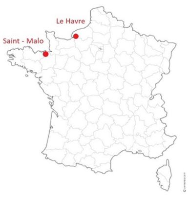
Figure 1The Saint-Malo and Le Havre sites.
As the study focuses on the integration of tidal range in a macrotidal environment in the calculation of the probability of joint occurrence of waves and water levels, the used data are those of waves and surges taken at high tide. The sample is made of 706 events per year using the same definition as in the Rock Manual. In coastal engineering, it is customary to calculate the probability of occurrence of extreme tidal sea levels by making the product of convolution of high tide densities with the survival function of storm surges. As 706 annual tides occur, the annual probability of exceeding a given level is chosen in reference to this figure of 1∕706. In addition, because coastal structures are located at shallow depths, the conditions that require the structures in terms of their stability or wave overtopping correspond to waves occurring with high water levels. That is why the privileged situations are high tides. The analysed samples are therefore pairs of storm surge associated with wave height at high tide. However, for safety, the wave height that is chosen is the maximum value over the 3 h time interval on either side of high tide. Kergadallan (2015) recommends selecting the maximum H value within a time window centred on the time of high water. Using the same data as him, this recommendation is followed. Statistical samples therefore contain tuples of wave and storm surge values at high tides at the rate of 706 annual pairs. Separated by about 12 h, the values may not fully meet the independent and identically distributed (i.i.d) assumption. However, this aspect is not considered here as it is often accepted in practice (see for example Hawkes, 2005).
Another approximation is the assumption of the presence of a unique wave population. This assumption is also not completely valid when we consider the wave direction of extreme events. The topic has already been discussed by Hawkes et al. (2002), Mazas (2019), and Mazas and Hamm (2017), among others. The treatment of wave direction can also be considered to be a fourth random variable of the oceanic forcing but has not been included in this work.
For low and moderate values the cumulative distribution functions (CDFs) FH, FT and FS are the empirical functions. For the strongest and extreme values, these cumulative distribution functions result from an adjustment of the exponential law. Survival functions, whether for storm surge or wave height, are therefore adjusted by piece by exponential-type analytical functions as close as possible to empirical frequencies, whereas extrapolations for extreme values use exponential laws.
2.2 Selection of the best bivariate copula by two methods
2.2.1 The error method
We illustrate the method for the random variables wave height H and storm surge S. This method consists of determining the mean error e between the calculated joint cumulative distribution function with the copula C, its parameter θ and the observed joint cumulative distribution function Fmes(h,s):
with n the number of pairs of values (hi, si).
For each copula, we first determine the parameter θ that minimizes the error e. We then select the copula with the lowest minimum mean error.
2.2.2 The maximum-likelihood method
Let us call X the sample of measures (x1, x2, …, xn) with bivariate , i=1, ..., n. The likelihood function L is defined by Eq. (2):
where fcal is the probability density function of the bivariate cumulative distribution function Fcal. θ is the parameter of the copula.
The maximum-likelihood method consists of finding the parameter θ, which maximizes the probability of obtaining the sample (Tassi, 2004). Since likelihood is a product of density we take its log-likelihood in order to facilitate calculations. We can thus work with the sum and derive it with respect to θ as shown below:
The best copula is the copula with the largest likelihood.
2.3 Construction of a trivariate copula
For more than two variables, C is not generally a copula (impossibility theorem of Genest, 1995). According to Nelsen (2006), it is difficult to construct n-order copulas from n−1 copulas. We present two methods for the construction of trivariate copulas. In the first method, a trivariate copula generalizes the bivariate copula with three random variables and one parameter. In the second method, a trivariate copula associates two bivariate copulas with their two respective parameters.
2.3.1 Definition of a copula in dimension d>2
A copula in dimension d is a distribution function on [0,1]d whose marginal laws are uniform on [0,1].
A copula is a function C: , which satisfies the following three conditions:
A function h: is called d-growing if for any hyper-rectangle [a,b] of Rd, , where
For each t, .
2.3.2 Trivariate copula with one parameter: a multi-level Archimedean trivariate
Since we are looking for the correlation between three variables, the first idea is to generalize the bivariate copula C(u1, u2) to obtain . We must check that is a copula, which is difficult. However Archimedean copulas like Gumbel and Clayton can be extended to an order greater than 2 using the property of Archimedean copulas (see Appendix A).
For a Clayton copula of order n, this gives
For Clayton copula of order 3, it gives
For Gumbel copula of order n, it gives
For Gumbel copula of order 3, it gives
By taking a single copula parameter for the three variables, we do not differentiate the pairwise correlations of the variables even though some variables may be more correlated than others.
2.3.3 Trivariate copula with two parameters: a fully nested hierarchical copula
To better take into account the correlations of variables two by two, one option is to build trivariate functions from bivariate copulas as a fully nested hierarchical copula as follows:
Corbella and Stretch (2013) tests a fully nested hierarchical copula, but he uses a unique bivariate copula and does not distinguish the two bivariate copulas C1 and C2. C1 is a bivariate copula with θ1 as copula parameter. C2 is a bivariate copula with θ2 as copula parameter. We must check that this function (Eq. 10) is a copula and satisfies the properties of Eq. (4). We first aggregate the two most correlated variables with the copula C2 and its copula parameter. We then add the third random variable with the copula C1 and its copula parameter. We show later that this order provides the most robust copula.
2.3.4 Validity of copula properties for Sect. 2.3.3
We do not know any general methods to build high-order copulas from low-order copulas (Durrleman, 2010). Generally is not a copula. To prove that is a copula, we must check that satisfies the three properties of Eq. (4) with d=3, which is difficult. However Charpentier (2014) points out that C is a copula if it satisfies (i) or (ii).
- i.
C1 and C2 are both Clayton or Gumbel copulas with parameters θ1 for C1 and θ2 for C2 and are positive and growing.
- ii.
C1 and C2 are both Archimedean copulas of respective generator ϕ1, ϕ2 with being the inverse of a Laplace transform.
For Gumbel and Clayton copulas C1 and C2 that are Archimedean copulas, we check the condition (ii) that there is a function f for which the inverse Laplace transform satisfies
with ϕ1, ϕ2 generators of the copulas C1 and C2. is the Laplace transform of f.
For C1 and C2 Clayton copulas we have as the generator of C2 and as the inverse generator of C1
This gives
We can find that
with Γ(a,x) the incomplete Gamma function set for a complex with real part (a) > 0
We conclude that there is a function f such that with
For C1 and C2 Gumbel copulas we have as the generator of C2 and as the inverse generator of C1
This gives
We can find that
with Γ Gamma function defined by
We conclude that there is a function f such that , with
2.4 Determination of the contour of equal joint exceedance probability
The determination of the contour of equal joint exceedance probability consists of obtaining all the variables (H, T, S) associated with different return periods: T10 (10-year event), T100 (100-year event) and T1000 (1000-year event).
2.4.1 Bivariate probability without tide
We deal with a set of pairs of values (h,s) that satisfy
is the selected bivariate survival copula. are survival functions associated with the variables. The values f10, f100 and f1000 are the frequencies corresponding to the 10-year, 100-year and 1000-year periods, i.e 1∕7060, 1∕70 600 and 1∕706 000.
2.4.2 Bivariate probability with tide
The bivariate probability with tide requires the development of the copula connecting wave height and storm surge. We can then define the joint survival function of the wave height and the storm surge. The chosen calculation method favours high tide. The sea levels considered are therefore the sums of the astronomical high tide (generated by the attraction of the moon and the sun without weather disturbance) and the storm surges raised at the time of these astronomical high tides. This method is of course valid only for macrotidal seas. The probability that the sea level at high tide N exceeds a given value n is expressed as follows:
with z the height of the high tide between the minimum and maximum values Mmin and Mmax, respectively, at high tide; fM(z)dz the probability that the high tide is between z and z+dz; and the probability of observing a storm surge S larger than s, thus . Equation (23) is established by Simon (1994).
The bivariate survival function for wave height H and sea level N is therefore written as follows:
Introducing the survival copula , the final equation is
The set of pairs (h,n) corresponding to the different return periods the 10-year, 100-year and 1000-year periods satisfies
It is thus possible to represent the contour of equal joint exceedance probability associated with the variables wave height and sea level.
2.4.3 Trivariate probability without tide
Here we have chosen the method of construction of a trivariate copula with two parameters known as fully nested hierarchical copula. We have
with and the selected bivariate survival copula. From Eqs. (27) and (28) we therefore obtain the equation that follows
The triplets of values () corresponding to the different return periods T10 (10-year event), T100 (100-year event) and T1000 (1000-year event) satisfy
It is thus possible to represent the contours of equal joint exceedance probability associated with the variables wave height, wave period and sea level.
2.4.4 Trivariate joint exceedance probability with tide
The trivariate survival function for wave height H, wave period T and sea level N is written as follows:
This can be written by introducing the selected survival copula :
Introducing the survival copula connecting and , the final equation is
The triplets of values () corresponding to the different return periods T10 (10-year event), T100 (100-year event) and T1000 (1000-year event) satisfy
It is thus possible to represent the contours of equal joint exceedance probability associated with the variables wave height, wave period and sea level with tide.
2.5 Tail dependence of the sample
It is necessary to treat the extreme events that are characterized by a very low occurrence. The difficulty of taking them into account is of a statistical nature: the scarcity of observations. In order to take the extreme events into account, we introduce the concept of tail dependence. For a bivariate copula, the tail dependence measures the probability of simultaneous extreme realizations (Clauss, 2008). It is a highly relevant tool for the study of extreme values. We distinguish lower- and upper-tail dependences. They are characterized by their lower- and upper-tail dependence coefficients that are deduced from the following conditional probabilities, whose value is given by Eqs. (35) and (36) that are given by Clauss (2008) for cumulative distribution functions U1 and U2:

Since we fix the lower-tail dependence coefficient λL and upper-tail dependence coefficient λU by equations
we deduce the definitions of tail dependence coefficients.
Definition: The lower-tail dependence coefficient is defined by
The copula C has a lower-tail dependence if λL exists with .
If λL=0 then the copula does not have a lower-tail dependence.
Definition: The upper-tail dependence coefficient is defined by
The copula C has an upper-tail dependence if λU exists with .
If λU=0 then the copula does not have an upper-tail dependence.
In the following section, we use survival copula and survival function . The lower-tail dependence corresponds then to high wave heights and water levels.
The tail dependences of the different copulas are determined in Nelsen (2006) and Roncalli (2002) from their tail dependence coefficients. They are expressed in Table 1. The Ali–Mikhail–Haq copula and Gaussian copula are noted AMH and Gauss, respectively, in what follows.
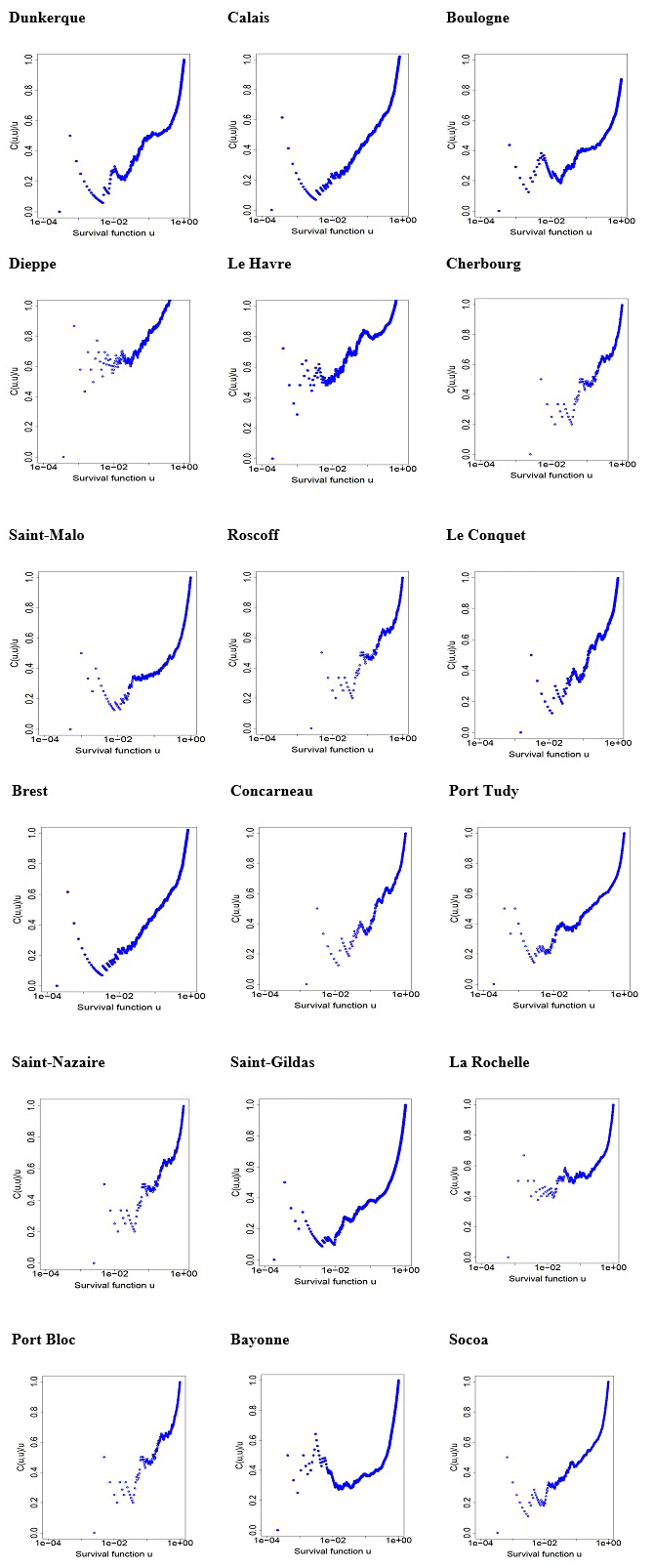
We find that some copulas do not have lower- and upper-tail dependence coefficients. They are inappropriate in case of extreme dependence. Some copulas have a lower-tail dependence; others have an upper-tail dependence. The tail dependence of the sample is firstly checked. For this we graphically represent the evolution of and determine its limit when tends to 0. Since is used, we note the tail dependence coefficients and . We can therefore decide whether the sample does or does not have a lower- or upper-tail dependence. In choosing the copula, it is essential to satisfy the class of tail dependence of the sample. If the sample does not have a tail dependence, then the use of the Gaussian copula or another copula with the same class or tail dependence is recommended. If the sample has a lower-tail dependence, the use of a copula with a lower-tail dependence or the survival copula with an upper-tail dependence is recommended. If the sample has an upper-tail dependence, the use of a copula with an upper-tail dependence or the survival copula with a lower-tail dependence is recommended. We can also deduce the parameter of the copula from the tail dependence coefficient given by the sample. The method that is proposed here for assessing the sample dependence refers to lower-tail dependence. Other methods exist such as the chi-plot proposed by Fisher and Switzer (1985, 2001) and used in coastal analyses by Mazas and Hamm (2017) for instance.

We select the most appropriate copulas at both the Le Havre and Saint-Malo (northern France) sites using two methods. We analyse the class of tail dependence of the two samples. We represent the contour of equal joint exceedance probability with the selected copulas for three return periods in order to assess the relevance of the copulas.
3.1 Statistical law for adjusting wave height, wave period and storm surge
The representation of the contours requires knowledge of the statistical laws of adjustment of the different parameters. We therefore present these laws. For the two sites of Saint-Malo and Le Havre, we have used data files that provide the values for wave height, wave period and storm surge at high tide over a time period of about 20 years. The file for the Le Havre site includes, for example, around 15 000 values. The wave data are extracted from the Anemoc numerical database. Sea levels at high tide are extracted from tide gauge measurements. The astronomical tide is obtained from the Shom Predit software.
Adjustments of the statistical laws are made according to the peaks-over-threshold (POT) method on the basis of the exponential law.
The copula parameters are calibrated from samples where wave height values less than 1 m are excluded (see Fig. 2), thus reducing the sample size to about 3000 values. The copulas are fitted to all pairs or triplets of observations where the wave height exceeds 1 m. This threshold of 1 m that is used for filtering wave height excludes the swells and leaves only a very homogeneous population of pure wind waves. This treatment removes long wave periods and increases the dependence between wave height and wave period.
3.2 Current pratice: Defra method
The use of the simplified Defra method in Ciria et al. (2007) is common among European coastal engineers for the study of wave overtopping or armour damages in coastal structures. It refers to the complete Defra method presented for example by Hawkes (2005) that is based on the Gauss copula. The complete Defra method is close to the method that is used in this paper. The main difference is the choice of the Gauss copula that does not present tail dependence. The simplified Defra method refers to univariate survival functions and rather than cumulative distribution functions of wave height and storm surge as coastal engineers usually work with exceedance probability rather than with non-exceedance probability. In this simplified method, the bivariate survival function is related to univariate survival functions by the expression
In France, the order of magnitude for the dependence factor FD coefficient is about 20. Kergadallan (2013) recommends however a minimum value of 25 for safety reasons. This factor corresponds to a weak dependence. For a very strong dependence, FD is between 500 and 1000.
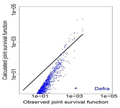
Figure 3Comparison of calculated (with Defra method) and observed joint frequency for Le Havre.
The bivariate survival functions of Table 4.15 of Rock Manual (Ciria et al., 2007) are determined with Eq. (41). Figure 3 shows the differences between observed bivariate survival functions and calculated bivariate survival functions using the simplified Defra method. The points of calculations in blue lie far from the first bisector in black in the figure. This shows that the use of the Defra simplified method is inappropriate. This is due mostly to the use of the simplified Defra method of Eq. (41), but the complete Defra method with the Gauss copula would not also perfectly represent the extreme events because the Gauss copula has no tail dependence, as we see later.
In order to improve the results, we now introduce the copula theory.
3.3 Analysis of the tail dependence
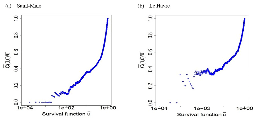
The sample is analysed in order to determine its tail dependence. Indeed, the result will condition the choice of the copula depending on whether the sample has the same class of tail dependence as the copula or not. In Eqs. (22), (26), (30) and (34), the survival copula is used with survival functions. In the following section, we use survival copula and survival function . Upper-tail dependence and lower-tail dependence will be inverted. We are interested in the extreme events with high wave heights and water levels. For survival copula , we determine below its limit for survival function tending to 0. The lower-tail dependence corresponds to these high wave heights and water levels.
For the Saint-Malo sample, tends to around 0.2 when tends to 0.
For the Le Havre sample, tends to around 0.4 when tends to 0.
Using the survival function , these two samples have a lower-tail dependence, which justifies the use of the Clayton copula. We determine the Clayton copula parameter from the lower-tail dependence coefficient of the sample. With the Clayton copula, we can determine the value of its copula parameter in Saint-Malo and Le Havre with the equation
This copula parameter is 0.43 and 0.76, respectively.
Note: as the Gumbel copula has an upper-tail dependence it is not recommended. In contrast, its survival copula with a lower-tail dependence is appropriate. This analysis of the sample makes it possible to understand why the survival Gumbel copula gives a minimum error close to the minimum error of the Clayton copula. We can therefore expect survival Gumbel copula results to be close to the results obtained by the Clayton copula.
3.4 Selection of the best bivariate copula for Le Havre and Saint-Malo samples
3.4.1 The log-likelihood method
For the set of survival copulas we determine their maximum likelihood with their parameter. We will select the survival copula with the largest likelihood among those which possess the same class of tail dependence as the sample with the largest likelihood. In bold in Table 2 are presented the survival copulas with a lower-tail dependence: Clayton, survival Gumbel and Student. AMH is added in bold when the copula parameter is close to 1. We come back later to this special property of the AMH copula. The Gauss copula has a relatively large likelihood. However, it does not have a tail dependence and therefore cannot correctly represent the tail dependence.
Table 2Copula parameter and maximum likelihood for the different survival copulas in Saint-Malo and Le Havre.
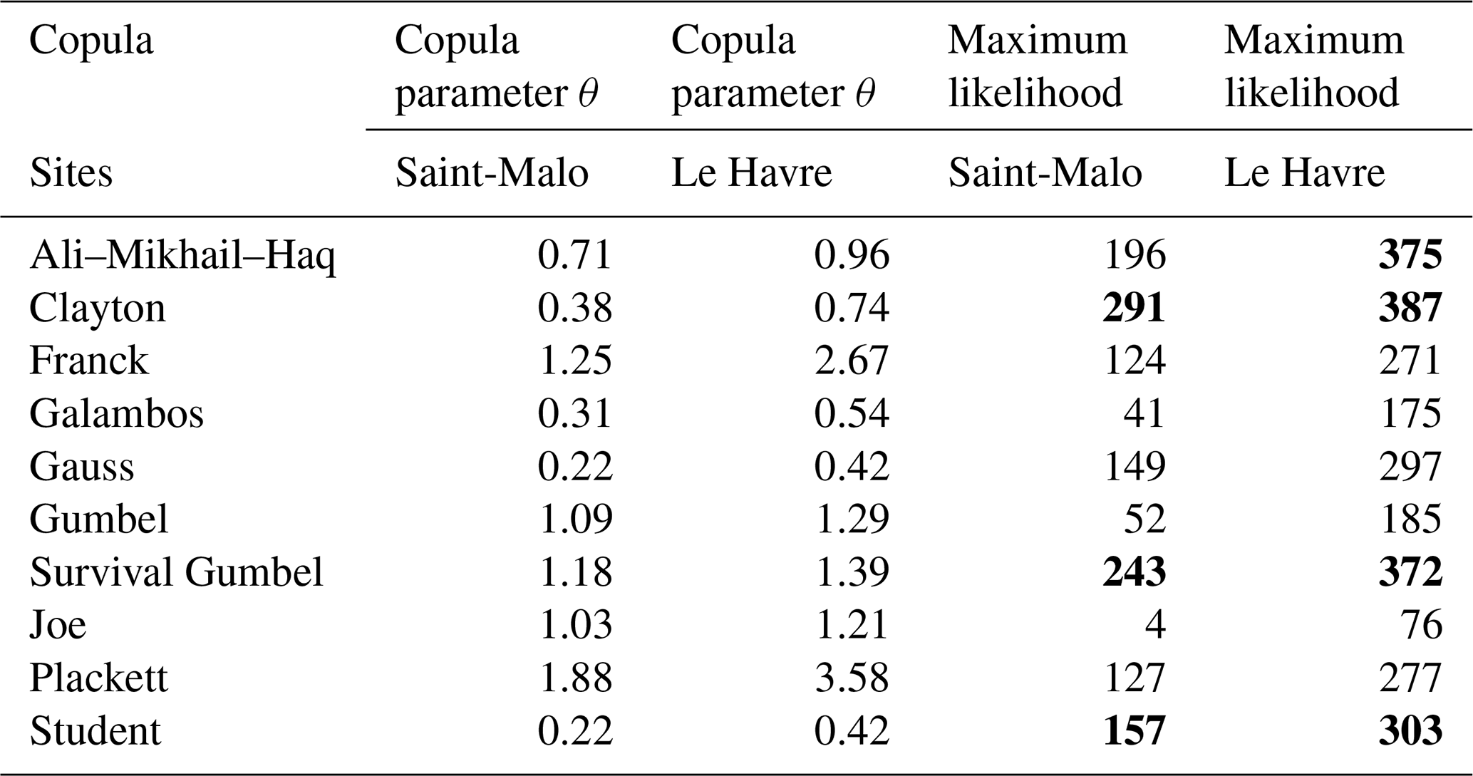
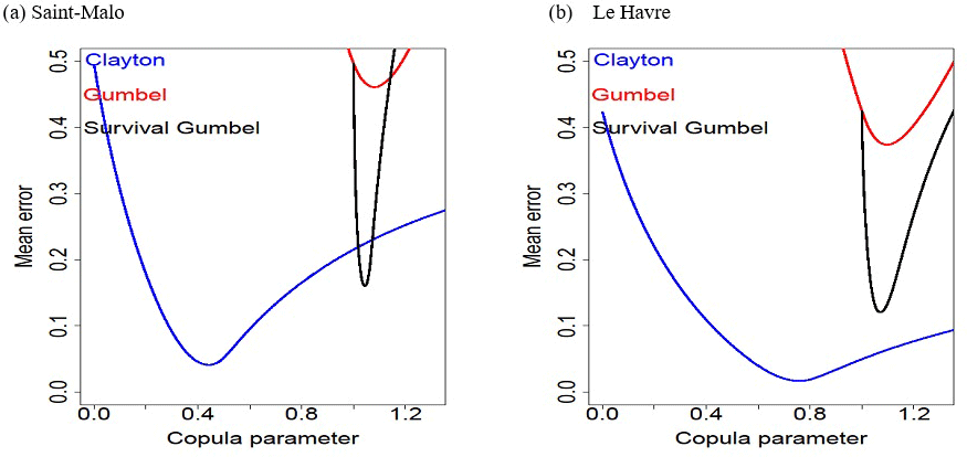
Figure 5Evolution of the error according to the Clayton, Gumbel and survival Gumbel copula parameter in (a) Saint-Malo and (b) Le Havre.
For the Saint-Malo sample, we choose the Clayton copula, which has the same class of tail dependence as the sample, with a log-likelihood of 291 in Table 2. For the Le Havre sample, we also choose the Clayton copula, which has the same class of tail dependence as the sample, with a log-likelihood of 387.
The Clayton copula parameters obtained by the tail dependence coefficients come close to those obtained by the log-likelihood method for the Le Havre sample (3040 values) and the Saint-Malo sample (5888 values).
For Saint-Malo, we obtain as 0.38 the parameter of the Clayton copula using the method of maximum likelihood and 0.43 with the tail dependence coefficient.
For Le Havre, we obtain 0.74 as the parameter of the Clayton copula using the method of maximum likelihood and 0.76 with the tail dependence coefficient.
Even if this comparison is satisfactory, the method can be sensitive to the data and the way to determine the limit. Caillault and Guegan (2005) propose for example two methods which allow the copula characterizing the bivariate distribution function of a pair of markets to be estimated. One method privileges the extreme behaviour of the bivariate distribution function of the pair, and the second one is based on the estimates of the copulas' parameter using a pseudo log-likelihood method. They conclude that the two approaches give different estimates of the tail dependence.
The value of the log-likelihood of the survival Gumbel copula is approximately as large as the log-likelihood of the Clayton copula. In addition, the survival Gumbel copula has the same class of tail dependence as the Clayton. It is therefore potentially as suitable as the Clayton copula.
3.4.2 The error method for the Clayton, Gumbel and survival Gumbel copula
In order to select the most relevant copula, we represent the mean error e between the calculated survival function with the copula C and its parameter and the measured Fmes(h,s).
Figure 5 for the ports of Saint-Malo and Le Havre shows that the error that is obtained with the survival Gumbel copula is very close to that obtained with the Clayton copula. The curve of the error obtained by the survival Gumbel copula however has a very acute minimum. Obtaining the parameter of this copula will therefore be very sensitive to the value of its minimum error. It will therefore be necessary to determine it very precisely.
Note: Gumbel and Clayton copula parameter supports are different and are [[ and ][, respectively.
Table 3Emin, error rate and copula parameter for the different survival copulas in the ports of Le Havre and Saint-Malo: Clayton, Gumbel and survival Gumbel.
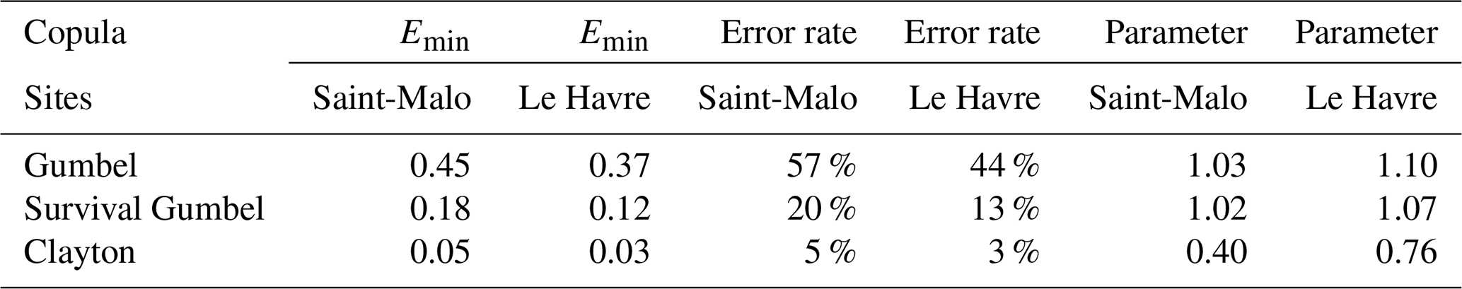
We note that Emin is the minimum of the mean error e and error rate + . Table 3 below shows the results obtained for Saint-Malo and Le Havre.
Table 3 is used to verify that the Clayton copula is the most robust copula. It appears that the survival Gumbel copula is also an appropriate option.
We have therefore shown by two methods that the Clayton copula is the most relevant for the Saint-Malo and Le Havre sites.
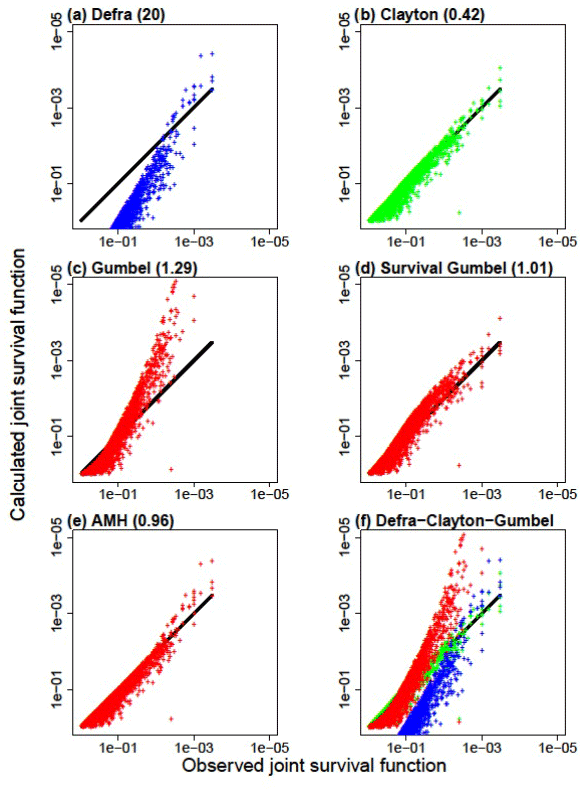
Figure 6Comparison of the observed joint survival and the calculated joint survival function for Le Havre with (a) the Defra method, (b) Clayton (0.42), (c) Gumbel (1.29), (d) Survival Gumbel (1.01), (e) AMH (0.96) and (f) Defra–Clayton–Gumbel.
The parameters of the copula obtained by the error method are close to those obtained by the method of maximum likelihood for the Clayton copula.
3.5 Comparison of observed and calculated joint frequencies
In order to assess the robustness of the copulas, we show in Fig. 6 the observed and calculated joint frequencies for the Le Havre sample (3 040 pairs of values). The copula represents reality more closely when the points approach the bisector y=x. The simplified Defra method currently in use does not give a good representation of the reality of the joint frequencies for wave height and storm surge. The Clayton copula provides a good representation. In contrast, the Gumbel copula gives a bad representation. The explanation is in the analysis of the sample carried out in Sect. 3.3: we show that the sample had a lower-tail dependence, whereas the Gumbel copula has an upper-tail dependence. In contrast, the survival Gumbel copula provides a good representation of the reality of joint frequencies for wave height and storm surge. The explanation lies in introducing the survival copula. The tail dependence of the survival Gumbel copula is opposite to the tail dependence of the Gumbel copula. The survival Gumbel copula therefore has the right class of tail dependence. The results obtained by the AMH copula are surprisingly correct. Kumar (2010) shows that the AMH copula does not have tail dependence except if the copula parameter is equal to 1. In our case, the copula parameter is close to 1. The copula therefore seems to behave like a copula with a lower-tail dependence. We show here the utility of the Clayton copula in comparison with the Gumbel copula and the Defra method that is currently in use.
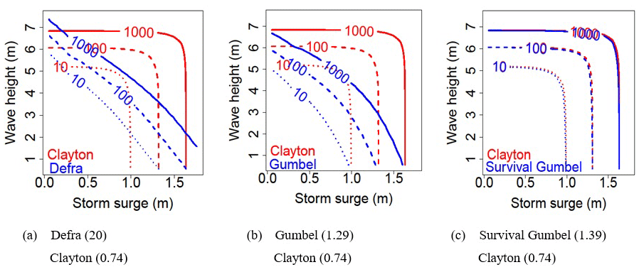
Figure 7Contours of equal joint exceedance probability with Clayton (0.74), Defra (20), Gumbel (1.29) and survival Gumbel (1.39) for return periods of 10, 100 and 1000 years for Le Havre.
The results highlight the importance of the class of tail dependence of the sample in copula selection. If the sample has a tail dependence it is necessary to select a copula with the same tail dependence. The Clayton copula that has the same class of tail dependence as the sample gives a calculated joint frequency close to the observed joint frequency. Conversely the Gumbel copula does not correctly represent the observed joint frequency: it moves away from the bisector for the extreme points. This is because the sample has a tail dependence opposite to that of the Gumbel copula. In order to restore the proper tail dependence, we resort to the survival copula. The latter comes close to the bisector but is slightly less robust than the Clayton copula. It should be noted that calibration is performed on the entire sample. By truncating the sample for joint frequency values below 0.01, we would have obtained a much larger parameter for the Gumbel copula with results that are closer to measurements.
3.6 Contours of equal joint exceedance probability with the bivariate copula
3.6.1 Contours without tide for the Clayton, Gumbel and survival Gumbel copulas and the Defra method
Figure 7 shows the joint exceedance probability (H,S) for the Le Havre (3040 values) samples, respectively, with Clayton, Gumbel and survival Gumbel copulas and the Defra method.
Figure 7a–c present the comparison of Clayton with, respectively, Defra, Gumbel and survival Gumbel. Contours of equal joint exceedance probabilities obtained by Clayton are very far from those obtained by Gumbel and the Defra method. In contrast, the joint exceedance curves obtained using the survival Gumbel copula are very similar to those obtained with Clayton. Results are therefore very sensitive to the choice of copula. A poor choice may lead to undersizing and may have economic consequences.
3.6.2 Contours with tide for the Clayton copula
Figure 8 shows the contours of equal joint exceedance probability, respectively, for the port of Saint-Malo (5000 tidal values) and the Le Havre sample (22 000 tidal values) with the Clayton copula.

Figure 8Joint exceedance probability obtained with (a) the Clayton copula (0.38) for Saint-Malo (b) with the Clayton copula (0.74) for Le Havre with tide for return periods of 10, 100 and 1000 years.
With tide the effect of storm surge on the sea level is small. The tidal range, which has an amplitude much larger than the storm surge, especially for the port of Saint-Malo, mitigates the variations due to the storm surge. In particular, for the port of Saint-Malo, it can be seen that sea level is less sensitive to variations in the return periods than storm surge (cf. Fig. 8).
3.7 Conclusion on selecting the best bivariate copula
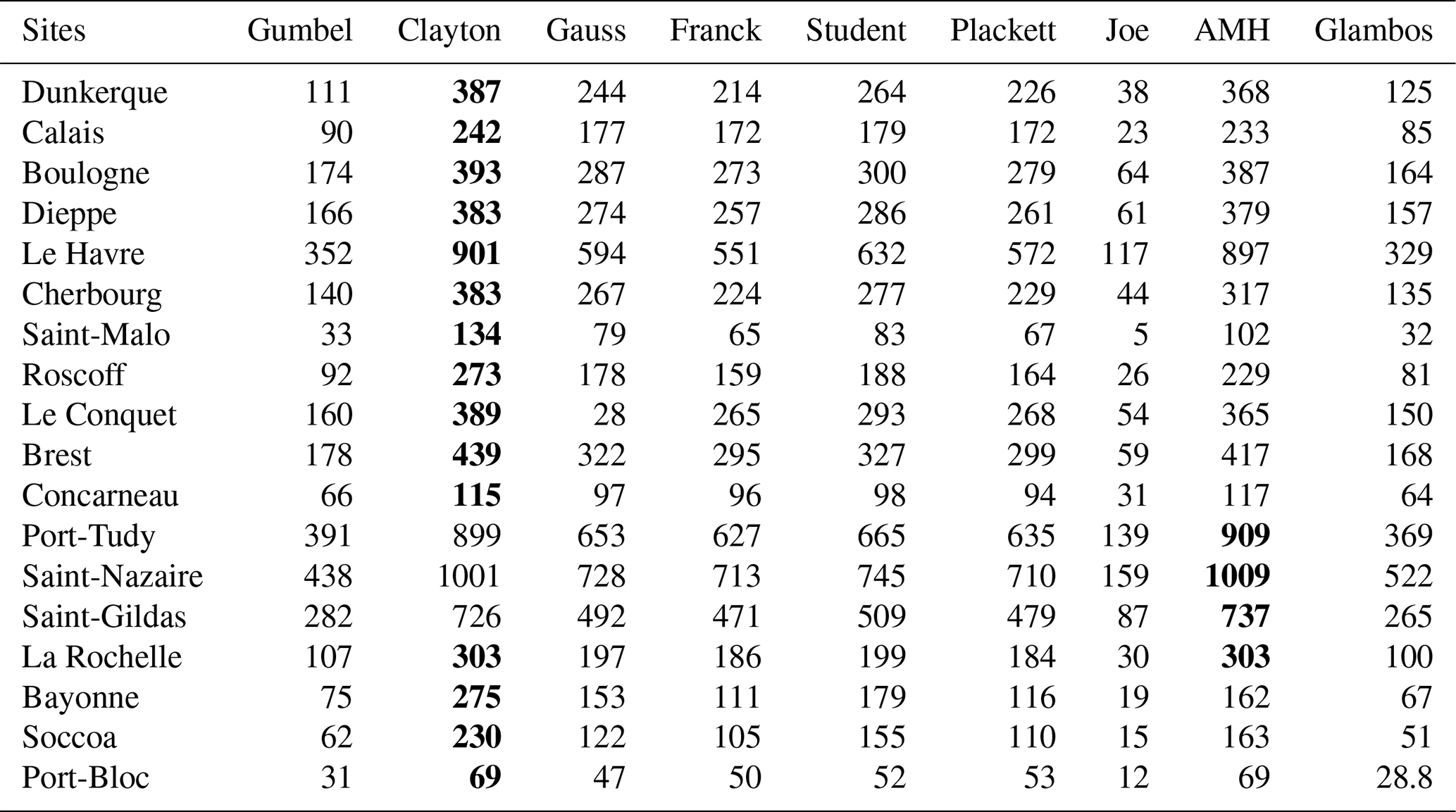
We selected the Clayton copula for the ports of Le Havre and Saint-Malo using three methods. In order to validate the Clayton copula, we analysed samples from 19 sites of the French coast along the Atlantic and English Channel with the maximum-likelihood method. We always obtained the greatest maximum likelihood with the Clayton copula or the AMH copula (see Appendix C). The sample always has lower-tail dependence (see Appendix B). Even though at some sites the AMH copula provides a larger likelihood than the Clayton copula, it should not be chosen because it has a particular kind of behaviour. It has a lower-tail dependence if the copula parameter is 1 (or close to 1 in practice). If the parameter is not 1, the AMH copula does not have tail dependence, and its interests disappear. Since the robustness depends on the copula parameter and on the site, it cannot be recommended for general use. We can therefore conclude that the Clayton copula is the most appropriate copula for our application. For this purpose, Table 4 gives the parameters of the different sites.
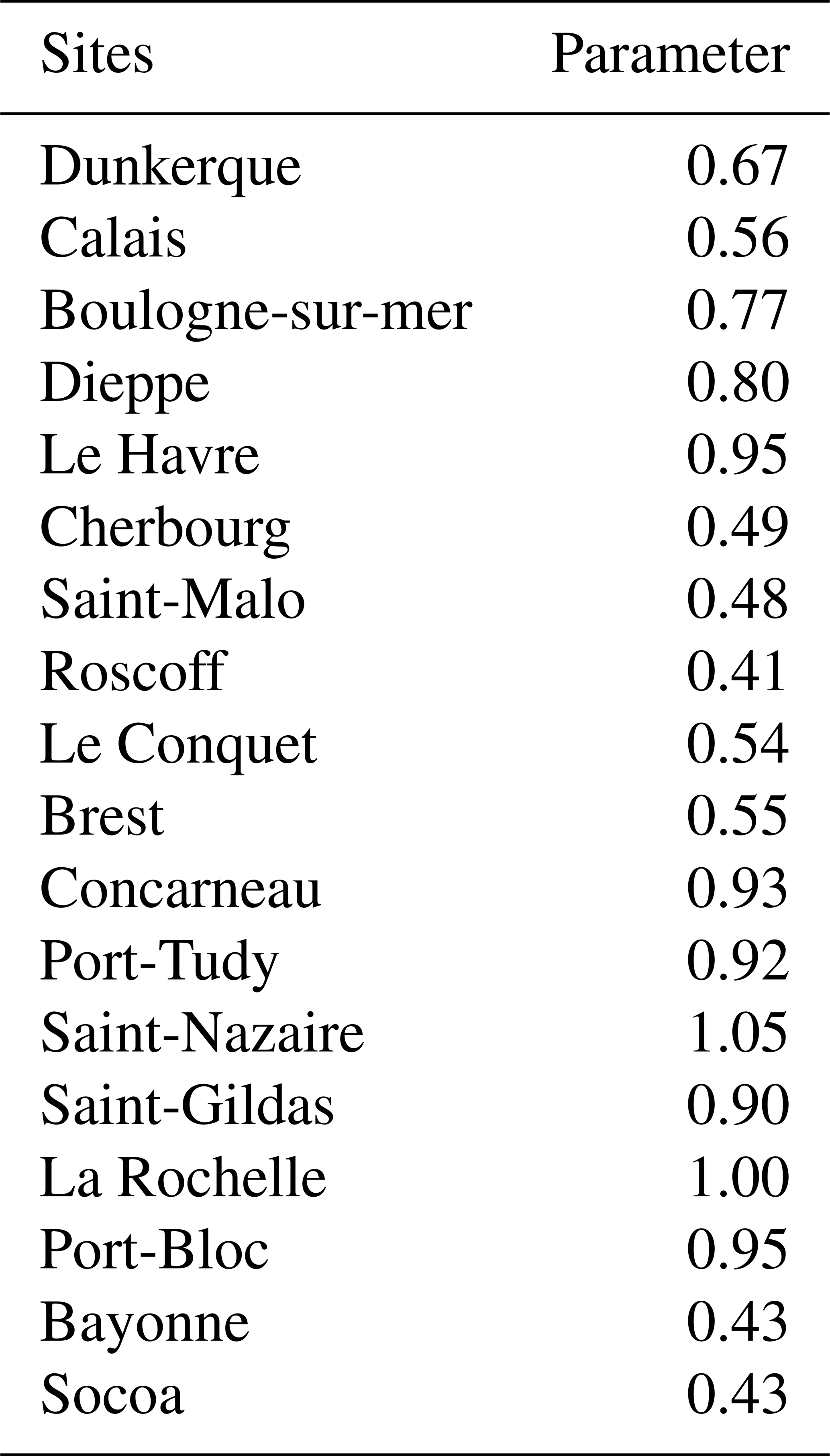

Figure 9The coast with the maximal dependence from Concarneau to Port-Bloc.
We show in Fig. 9 that there is a coastal area with a maximal dependence from Concarneau to Port-Bloc (in grey in the figure). This area is the most exposed to wind that comes mainly from the west direction along the French Atlantic coast.
4.1 Methodology
We have tested hierarchical construction using a fully nested hierarchical Archimedean copula. In this type of construction, we build a bivariate copula between two variables; then we create a trivariate copula with the previous copula and the third variable using another bivariate copula. Unlike Corbella and Stretch (2013), who uses the same copula parameter for the two bivariate copulas, we introduce two different copula parameters.
4.2 Construction of the best trivariate copula for the port of Le Havre
With the fully nested hierarchical copula method, we first determine the most appropriate bivariate copula for the three variables: (T,S), (H,T) and then (H,S). We construct the bivariate distribution function using the selected copula for the two most correlated variables. We determine the most relevant copula between the function obtained with the two most correlated variables and the third variable.
4.2.1 Bivariate copula for the three random variables
To determine the best bivariate copula we assess the maximum likelihood between (, , (, and (, with the different copulas in Table 5.
Table 5Log-likelihood and copula parameter for the different bivariate copulas between the parameters H and S, T and S, and H and T.
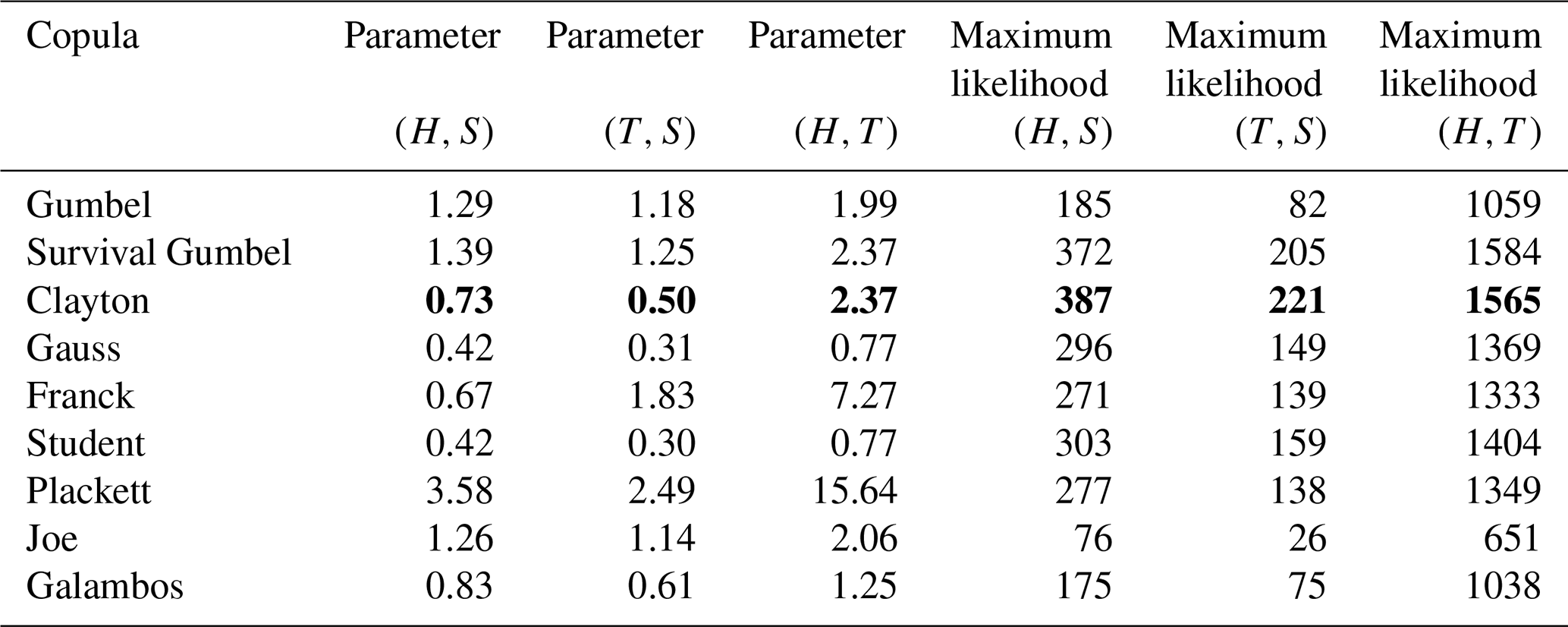
For all three combinations, the Clayton copula and survival Gumbel copula still have the largest maximum-likelihood value. In addition, we find that for the combination (H,T) the log-likelihood is significantly higher. This result is related to the fact that the parameters (H,T) are the most correlated parameters all the more since we deal with a very homogeneous population of pure wind waves, as noted in Sect. 3.1.
We can write
4.2.2 Determination of the best trivariate copula
We determine the maximum likelihood between and with the different copulas in Table 6.
Table 6Log-likelihood and copula parameter for different bivariate copulas between and .
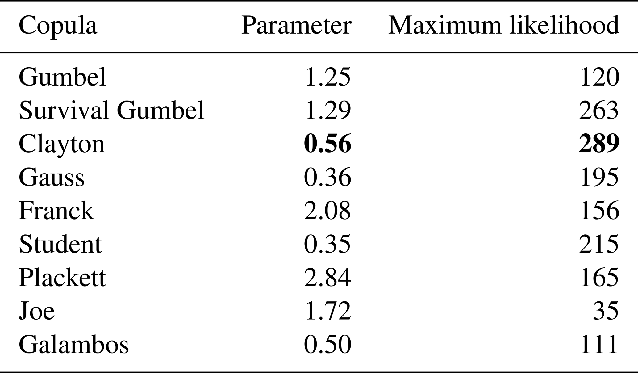
We obtain the largest log-likelihood for the Clayton copula, with a parameter of 0.56, which gives
In conclusion, we have thus aggregated the most correlated H and T parameters with the best-performing Clayton copula. We also used the Clayton copula to aggregate and . The aggregation requires two different parameters.
4.3 Contours of equal joint exceedance probability with a trivariate copula
We represent in Fig. 10 trivariate joint exceedance probability for return periods of 10, 100 and 1000 years. The trivariate copula used is therefore constructed from a Clayton copula parameter 2.37 connecting H and T and a copula parameter 0.56 connecting FHT and FS.
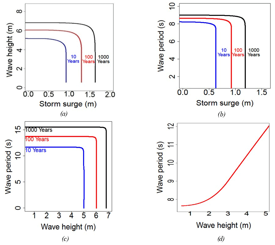
In order to better visualize the incidence of return periods on trivariate joint exceedance probability, cross sections along (H,T), (H,S) and (T,S) are shown for T=T1, H=H1 and S=S1 in Fig. 10a–c, respectively.
In Fig. 10a–c, a constant wave period, a constant wave height and a constant storm surge, respectively, are fixed corresponding to an annual return period. We show the joint exceedance probability of wave height and storm surge, of storm surge and wave period, and of wave height and wave period, respectively, for three return periods of 10, 100 and 1000 years. In the three figures we recognize the usual pattern and the characteristics of a strong correlation for (H,T). In Fig. 10c we recognize indeed the classic pattern of contours for very dependent variables. Wave height and wave period are the most correlated variables. This result is not surprising all the more since we deal with pure wind waves after we have removed the swell. In Fig. 10d, a relationship between H and T is obtained with a trivariate copula with (H,S) satisfying a joint exceedance probability of 1000 years and with T, which maximizes the trivariate joint probability density function. This relationship enables us to obtain the wave period from the wave height and the storm surge.
4.4 Error rate and goodness of fit for trivariate copulas
In order to show the utility of the constructed trivariate copula, we determine the error rate of the different copulas in the Le Havre area using the formula of the error given by Eq. (1) and the definition of the error rate given by exp (e)−1 (see Table 7).
Table 7Error rate of the different trivariate copulas for the port of Le Havre.

The results obtained by the trivariate copula constructed by two bivariate copulas and two parameters are the best of the four fitted trivariate copulas. However, by aggregating the most correlated variables first, the robustness improves, as stated by Charpentier (2014).
As expected, with one parameter the Archimedean copula is less robust than the fully nested hierarchical copula with two parameters.
It can also be seen that by associating the most correlated variables (H,T), the Clayton copula gives better results than the Gumbel copula. For a single parameter the trivariate copula constructed with the Clayton copula is significantly more accurate than the Gumbel copula.
Finally, Table 7 shows that the choice of the copula is much more important than the choice of the trivariate method of construction. This result validates our choice of a simple method of construction that can even lead to the most robust results according to Corbella and Stretch (2013).
Table 8Goodness of fit of the trivariate copulas for the port of Le Havre.

Table 8 presents the goodness of fit of the trivariate copulas for the port of Le Havre through the chi-squared test (CHI-2) and the Kolmogorv–Smirnov test (KS). The best results are obtained with two parameters. As expected, the fit of the single-parameter Archimedean copula and of the fully nested hierarchical copula is exactly the same copula as shown in Table 8. The results highlight the contribution of trivariate copulas constructed as a fully nested hierarchical copula with the help of two Clayton bivariate copulas and two parameters by first aggregating the two most correlated parameters.
Wave structure designers must accurately estimate return periods of parameters such as storm surge, wave height and wave period and, more specifically, their joint probabilities of exceedance. In engineering projects, this joint probability of exceedance is often related to the product of univariate probabilities by means of a simple factor. This method can cause damaging design errors. After highlighting the limitation of the current simplified Defra method, the theory of copula is introduced. Copulas make it possible to couple the marginal laws in order to obtain a multivariate law.
Analysis of the tail dependence of the sample is used to make an initial selection of the copulas. This is because if the sample has lower-tail dependence (upper-tail dependence, respectively), the copula with the same class of tail dependence or an inverse tail dependence is chosen by taking the survival copula. The correlation between the storm surge and wave height is modelled using the Clayton copula and the survival Gumbel copula.
In order to take into account the three variables (wave height, wave period and storm surge), we show that a fully nested hierarchical trivariate copula with two parameters is the best construction technique. This function satisfies the mathematical properties of the copulas. The error rate of 3.8 % is lower than the trivariate copula obtained by generalizing the Clayton copula with a single parameter (error rate of 8.8 %). We confirm that the best results are obtained by first aggregating the most correlated variables, which here are wave height and wave period. Nevertheless, the choice of method of aggregation is much less important than the choice of the copula.
A1 Bivariate cumulative distribution function
We denote by FX the cumulative distribution function (CDF) of a random variable defined by
where P is the probability.
We also introduce the survival function (SF) denoted by and defined by
The survival function is related to the probability density function fX by
Our objective is to obtain the bivariate cumulative distribution function or the bivariate survival function . For more information, the reader may refer to Dodge (1999), Revuz (1997), Ouvrard (1998) and Manoukian (1986).
We must model the correlation between, for example, wave heights H and storm surges S by proposing a relation defining the joint cumulative distribution function from the univariate cumulative distribution functions. We thus seek to obtain a function C which links the bivariate cumulative distribution frequency FXY(x,y) to the univariate cumulative distribution frequencies FX(x) and FY(y) by integrating a correlation parameter as follows:
A2 Current practice in coastal engineering
The simplified Defra method that is presented for example in Ciria et al. (2007) makes it possible to directly connect the joint probability density function fXY to the product of the univariate probability density functions fX and fY through a dependence factor, denoted FD, as follows:
The dependence factor FD depends on the correlation coefficient ρ obtained from the Gaussian copula (see definition in Sect. A.3.2). The variables X and Y for the bivariate analysis are generally wave height H and storm surge S. The dependence factor is region-specific and results from the analysis of the local correlation between wave heights and storm surges.
The correspondence table between the correlation coefficient ρ and the dependence factor FD is given by Kergadallan (2013). This table recommends, for example, for the North Sea, English Channel and Atlantic coast the use of a minimum dependence factor FD of 25 that is a weak dependence.
A3 Copulas
The copula is a statistical tool to characterize the dependence between several random variables where linear correlations are generally not able to represent them accurately (Charpentier, 2014). According to the latter, copulas have become an important tool for modelling a multivariate law that “couples” univariate cumulative distribution functions, hence the Latin name “copula” chosen by Sklar (1959).
If C is the copula associated with a random variable vector (X,Y), then the copula C couples the univariate cumulative distribution functions FX(x) and FY(y) using Eq. (A4).
Survival functions can also be coupled in the sense that there exists a survival copula such that
The survival copula is defined from the copula C as follows:
In the following description, the univariate cumulative distribution functions FX(x) and FY(y) are noted u1 and u2, respectively. A copula is a function C : which satisfies the following three conditions:
In the continuation of the paragraph on the description of the copula, the functions of distribution FX(x) and FY(y) are noted u1 and u2
Sklar (1959) states that there exists a copula C such that for each x and y . If the functions FX and FY are continuous, then C is unique. Four commonly applied copula families are the Archimedean, Elliptic, Marshall–Olkin and Archimax.
A3.1 Archimedean copulas
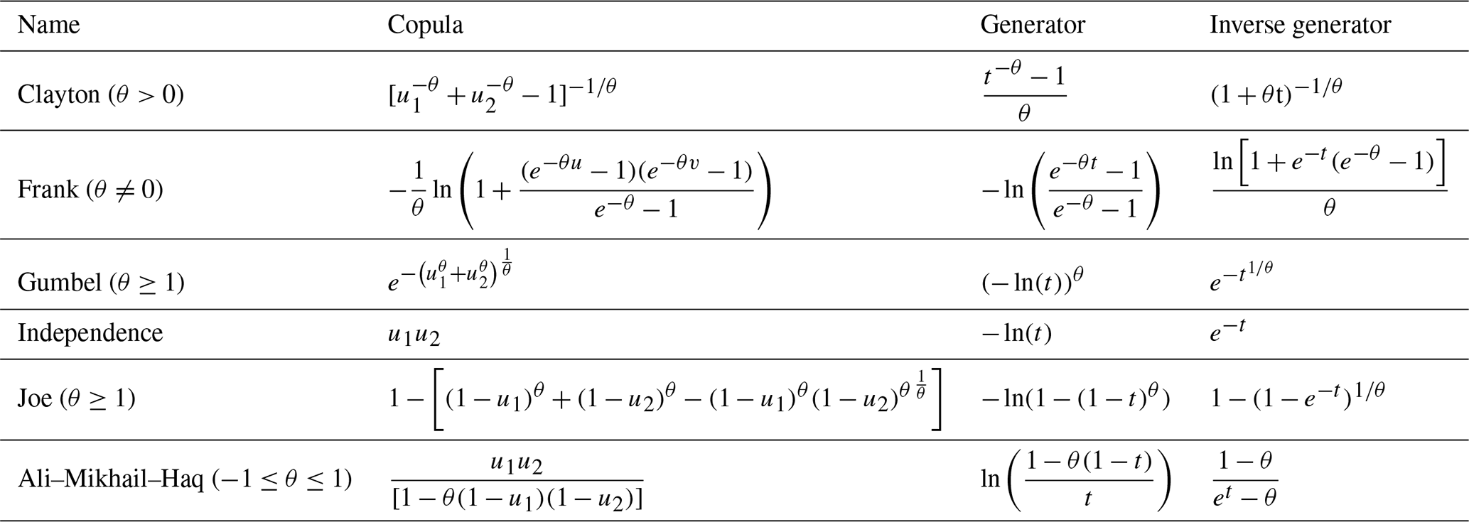
Archimedean copulas are defined as follows: ϕ is a decreasing function convex on , as ϕ(1)=0 and ϕ(0)=∞. We call a strict Archimedean copula of generator ϕ the copula defined as follows:
Archimedean copulas have interesting properties, in particular the possibility of aggregating more than two variables as follows:
Archimedean copulas are given in Table A1.
A3.2 Elliptic copulas
Elliptic copulas are Gaussian and Student's copulas.
The Gaussian copula is written as follows:
where ϕ is a distribution function of Xi, with a Gaussian random vector (), where ∑ is a covariance matrix.
Student's copula is written as follows:
with tν a distribution function of the univariate Student distribution law with ν degrees of freedom.
They are symmetrical copulas. They are widely used in finance. They are implicit and therefore do not have an explicit analytical form.
A3.3 Marshall–Olkin copula
Marshall–Olkin copula is written as follows:
A3.4 Archimax copulas
Archimax copulas include a large number of copulas, including Archimedean copulas.
A bivariate function is an Archimax copula if and only if it is of the form
A: such as for each t .
ϕ: is a convex, decreasing function that satisfies ϕ(1)=0.
We adopt the following notation: .
For more information, refer to reference books such as Joe (1997) and Nelsen (2006). The reader may also refer to Clayton (1978).
The used data can be accessed through http://anemoc.cetmef.developpement-durable.gouv.fr/doc/?p=conditions (ANEMOC, 2020; for waves), http://refmar.shom.fr/fr/partenaires/producteurs-de-donnees/reseau-maregraphique-ronim (RONIM, 2020; for sea levels) and https://maree.shom.fr/ (MAREES, 2020; for tides).
OO made applications in the programming language R. PS and FR proposed theoretical contributions and took part in writing the article.
The authors declare that they have no conflict of interest.
This article is part of the special issue “Advances in extreme value analysis and application to natural hazards”. It is a result of the Advances in Extreme Value Analysis and application to Natural Hazard (EVAN), Paris, France, 17–19 September 2019.
This paper was edited by Thomas Wahl and reviewed by two anonymous referees.
Aas, K. and Berg, D.: Models for construction of multivariate dependence – a comparison study, Eur. J. Financ., 15, 639–659, 2009.
Aghakouchak, A., Bardossy, A., and Habib, E.: Conditional simulation of remotely sensed rainfall data using a non-Gaussian v-transformed copula, Adv. Water Resour., 33, 624–634, 2010.
ANEMOC Atlas Numérique d'Etats de Mer Océanique et Côtier by Cerema, available at: http://anemoc.cetmef.developpement-durable.gouv.fr/doc/?p=conditions, last access: 31 January 2020.
Caillault, C. and Guegan, D.: Empirical estimation of tail dependence using copulas. Application to Asian markets. Quantitative Finance, Taylor & Francis, Routledge, 5, 489–501, 2005.
Chakak, A. and Koehler, K. J.: A strategy for constructing multivariate distributions, Commun. Stat. Simulat., 24, 537–550, 1995.
Chang, J., Li, Y., Wang, Y., and Yuan, M.: Copula-based drought risk assessment combined with an integrated index in the Wei River Basin, China, J. Hydrol., 540, 824–834, 2016.
Charpentier, A.: Copules et risques multiples, Approches statistiques du risque, Éditions Technip, Paris, 2014.
CIRIA, CUR, and CETMEF: Rock Manual: The use of rock in hydraulic engineering, second edn., C683, CIRIA, London, 2007.
Clayton, D. G.: A model for association in bivariate life tables and its application in epidemiological studies of familial tendancy in chronic disease incidence, Biometrika, 65, 141–151, 1978.
Clauss, P.: Théorie des copules, ENSAI, 2008.
Corbella, S. and Stretch, D.: Simulating a multivariate sea storm using Archimedean copulae, Coast. Eng., 76, 68–78, https://doi.org/10.1016/j.coastaleng.2013.01.011, 2013.
De Michele, C. and Salvadori, G.: A generalized pareto intensity-duration model of storm rainfall exploiting 2-copulas, J. Geophys. Res.-Atmos., 108, https://doi.org/10.1029/2002JD002534, 2003.
Dodge Y.: Premiers pas en statistiques, Springer-Verlag, Paris, 428 p., available at: https://www.springer.com/gp/book/9782287302787 (last access: 31 January 2020), 1999.
Durrleman, V.: Les fonctions copules. Définition exemples et propriétés. Cours de l'Ecole Polytechnique, Ecole Polytechnique, Palaiseau, 28 p., 2010.
Favre, A. C., El Adlouni, S., Perreault, L., Thiémonge, N., and Bobée B.: Multivariate hydrological frequency analysis using copulas, Water Resour. Res., 40, https://doi.org/10.1029/2003WR002456, 2004.
Fisher, N. I. and Switzer, P.: Chi-plots for assessing dependence, Biometrika, 72, 253–265, 1985.
Fisher, N. I. and Switzer, P.: Graphical assessment of dependence: is a picture worth 100 tests?, Am. Stat., 55, 233–239, 2001.
Genest, C.: De l'impossibilité de construire des lois à marges multidimensionnelles données à partir de copules, Comptes rendus de l'académie des sciences de Paris, 320, 723–726, 1995.
Genest, C. and Favre, A. C.: Everything you always wanted to know about copula modeling but were afraid to ask, J. Hydrol. Eng., 12, 347–368, 2007.
Gouldby, B., Méndez, F. J., Guanche, Y., Rueda, A., and Mínguez, R.: A methodology for deriving extreme nearshore sea conditions for structural design and flood risk analysis, Coast. Eng., 88, 15–26, 2014.
Grimaldi, S. and Serinaldi, F.: Design hyetograph analysis with 3-copula function, Hydrolog. Sci. J., 51, 223–238, 2006.
Hawkes, P. J.: Use of Joint Probability Methods in Flood Management: A Guide to Best Practice, Defra/Environment Agency and Flood and Coastal Defence R&D Programme, Defra – Flood Management Division, London, 2005.
Hawkes, P. J., Gouldby, B. P., Tawn, J. A., and Owen, M. W.: The joint probability of waves and water levels in coastal engineering design, J. Hydraul. Res., 40, 241–251, 2002.
Jane, R., Cadavid, L., Obeysekera, J., and Wahl, T.: Multivariate statistical modelling of the drivers of compound flood events in south Florida, Nat. Hazards Earth Syst. Sci., 20, 2681–2699, https://doi.org/10.5194/nhess-20-2681-2020, 2020.
Joe, H.: Multivariate models and dependence concepts, Ed. Chapman & Hall/CRC, Boca Raton, USA, 1997.
Kergadallan, X.: Analyse statistique des niveaux d'eau extrêmes, CETMEF, Compiègne, France, 179 p., 2013.
Kergadallan, X.: Estimation des niveaux marins extrêmes avec et sans l'action des vagues le long du littoral métropolitain (Doctoral dissertation), Université Paris-Est, Marne-la-Vallée, France, 2015.
Kumar, P.: Probability Distributions and Estimation of Ali-Mikhail-Haq Copula, Applied Mathematical Sciences, 4, 657–666, 2010.
Lee, T., Modarres, R., and Ouarda, T. B. M. J.: Data-based analysis of bivariate copula tail dependence for drought duration and severity, Hydrol. Process., 27, 1454–1463, 2013.
Li, Y., Simmonds, D., and Reeve, D.: Quantifying uncertainty in extreme values of design parameters with resampling techniques, Ocean Eng., 35, 1029–1038, https://doi.org/10.1016/j.oceaneng.2008.02.009, 2008.
Manoukian, E. B.: Guide de statistique appliquée, Herman, Editions Hermann, Paris, France, 202 p., 1986.
MAREES Horaires des marées by Shom, https://maree.shom.fr/, last access: 31 January 2020.
Mazas, F.: Extreme events: a framework for assessing natural hazards, Nat. Hazards, 98, 823–848, 2019.
Mazas, F. and Hamm, L.: An event-based approach for extreme joint probabilities of waves and sea levels, Coast. Eng., 122, 44–59, https://doi.org/10.1016/j.coastaleng.2017.02.003, 2017.
Nelsen, R. B.: An introduction to Copulae, Springer Series en Statistics, 269 p., 2006.
Ouvrard, J. Y.: Probabilités, Capes et aggregation, Cassini, Paris, 247 p., 1998.
Revuz, D.: Probabilités, Herman, Paris, France, 301 p., 1997.
Roncalli, T.: Gestion des risques multiples, cours ENSAI, available at: http://www.thierry-roncalli.com/download/Lecture-Notes-Copula-Ensai.pdf (last access: 31 January 2020), 219 p., 2002.
RONIM Réseau d'Observation du NIveau de la Mer by Shom, http://refmar.shom.fr/fr/partenaires/producteurs-de-donnees/reseau-maregraphique-ronim, last access: 31 January 2020.
Salvadori, G., De Michele, C., Kottengoda, N., and Rosso, R.: Extremes in nature. An approach using copulae, Water Science and Technology library, 56, Springer, Dordrecht, 2007.
Serinaldi, F.: Dismissing return periods!, Stoch. Env. Res. Risk A., 29, 1179–1189, https://doi.org/10.1007/s00477-014-0916-1, 2015.
Sergent, P., Prevot, G., Mattarolo, G., Brossard, J, Morel, G., Mar, F., Benoit, M., Ropert, F., Kergadallan, X., Trichet, J., and Mallet, P.: Adaptation of Coastal Structures to Mean Sea Level Rise, Houille Blanche, 6, 54–61, 2014.
Simon, B.: Statistique des niveaux extrêmes le long de la côte de France, Rapport d'étude n 001/94, Service Hydrographique et Océanographique de la Marine (SHOM), Brest, France, 1994.
Sklar, A.: Fonction de répartition à n dimensions et leurs marges, Publications de l'Institut de Statistiques de l'Université Paris, 229–231, 1959.
Tassi, P.: Méthodes statistiques. Collection Economie et statistiques avancées, Edition Economica, Paris, 2004.
Tilloy, A., Malamud, B. D., Winter, H., and Joly-Laugel, A.: Evaluating the efficacy of bivariate extreme modelling approaches for multi-hazard scenarios, Nat. Hazards Earth Syst. Sci., 20, 2091–2117, https://doi.org/10.5194/nhess-20-2091-2020, 2020.
Zhang, L. and Singh, V. P.: Trivariate flood frequency analysis using the Gumbel Hougaard copula, J. Hydrol. Eng., https://doi.org/10.1061/(ASCE)1084-0699(2007)12:4(431), 2007.
- Abstract
- Introduction
- Theoretical approach
- Results for bivariate copulas
- Results for trivariate copulas
- Conclusions
- Appendix A: Outlines of copula theory
- Appendix B: Tail dependence of the site
- Appendix C: Likelihood for 18 French sites
- Data availability
- Author contributions
- Competing interests
- Special issue statement
- Review statement
- References