Space-time clustering of climate extremes amplify global climate impacts, leading to fat-tailed risk

We present evidence that the global juxtaposition of major assets relevant to the economy with the space and time expression of extreme floods or droughts leads to a much higher aggregate risk than would be expected by chance. Using a century-long, globally gridded time series that indexes net water availability, every year we compute local occurrences of an extreme “dry” or “wet” condition for a specified duration and return period. A global exposure index is then derived for major mining commodities by weighting extreme event occurrence by local production exposed. We note significant spatial and temporal clustering of exposure at the global level leading to the potential for fat-tailed risk associated with investment portfolios and supply chains. This may not be a surprise to climate scientists familiar with the space-time patterns of interannual to decadal climate oscillations that can affect remote regions through teleconnections. However, the traditional approach of climate risk analysis only considers local or point extreme value analysis and hence does not account for temporal and spatial clustering of exposure for global portfolios. As multinational enterprises and supply chains assess and disclose physical climate risks, they need to consider the much higher chance that they may have multiple assets that may be exposed to extreme wet and/or dry climate extremes in the same year.

1 Introduction

A changing climate brings concerns as to whether there will be increasing business and societal disruptions, as well as conflicts associated with increasing water scarcity or flooding. Even if there were no significant impact of climate change, the growing world population and urbanization lead to increasing resource demands and imbalances whose changing exposure to climate risk needs to be understood. Yet, there are very few analyses (Bonnafous et al., 2017a, b) of the aggregate global annual exposure to hydroclimatic extremes over the last century for specific industries, activities, or population. Given the nonstationary nature of climate extreme occurrence and the intersection between the spatial structure of climate events and the concentration of human activity, there is potential for high risk. This climate risk remains even if structural or financial instruments (e.g., insurance) were used to mitigate it at each location, as is the norm. Typically, these instruments are designed based on the prior local climate record. Sometimes local information on local climate cycles (see for instance Khalial et al., 2007) or non-stationarity in event modeling (e.g., Lima et al., 2015; Hanel et al., 2009) is used. The implication at the portfolio level could be a fat-tailed, systemic risk for global enterprises.

From the perspective of a global investor or of a development or humanitarian aid agency, an assessment of the potential occurrence of many extreme hydroclimatic events across the planet in a given year is needed to assess potential supply chain risks, production shortfalls, conflict or needs for humanitarian relief. The World Bank noted that its development efforts can be compromised by climate extremes and climate change (World Bank, 2014). The 2011 floods in Thailand, the 2010 floods in Queensland and Pakistan, the 2014–2016 drought in São Paolo, and the 2016–2018 drought in Cape Town drew attention to their supply chain risk implications, as well as the potential for the disruption of tourism and global business. An area where the impacts of climate risk on global production has been highlighted is agriculture (USDA, 2010; Piao et al., 2010). Drought led to restrictions on exports of rice from key producing countries in 2008, leading to a doubling of the global price (Slayton, 2009; Bradsher, 2008). In this paper, we focus on another area of the economy, mining, but also show some results for urban areas and four major crops as a reference in the Supplement. We consider global socioeconomic exposure to the nominal once in 10-year local hydroclimate extreme for the annual production of four major mining commodities (using 2014 and 2013 production data) (SNL, 2016) at the major mining locations that represent a significant part (between 53 % and 78 %) of global production. Both dry and wet events are considered for mining given the potential additional expense on water sourcing in a drought and mine dewatering in wet years. The intention is to illustrate the nature of global exposure using a few globally relevant commodities.

2 Data and methods

The evolution through time of wet and dry extremes has primarily been studied through indices derived directly from precipitation (P) time series and through relationships between P, evapotranspiration (E), potential evapotranspiration (E_p), soil moisture (SM), runoff (R) and drought indices such as the Palmer Drought Severity Index (PDSI) and the Standardized Precipitation–Evapotranspiration Index (SPEI). The SPEI (Beguería et al., 2010, 2014) is a scalar index reported monthly. It is built after fitting a distribution on the cumulative P–E_p over a window of interest (e.g., 12 months). The dataset used is based on Climate Research Unit (CRU) (Harris et al., 2014) data for both precipitation and potential evapotranspiration and is accessible at http://spei.csic.es/database.html (last access: 7 March 2021). CRU is a gridded dataset with $\mathrm{0.5}{}^{\circ }\times \mathrm{0.5}{}^{\circ }$ spatial resolution of monthly temperature and precipitation built using the interpolation of station network data, which are accessible at https://crudata.uea.ac.uk/cru/data/hrg/ (last access: 7 March 2021). The SPEI is thus a measure of the net water supply, as estimated using local precipitation and potential evapotranspiration, over specified durations. We chose to use the SPEI for our analysis since a global reconstruction of this index covering 1901–2014 that has been well verified was available at a grid resolution of 0.5^∘. Since we are interested in an annual exposure, we used the 12-month duration values of the SPEI. We limit our analyses to the land area bounded by 60^∘ S to 60^∘ N and retain grid blocks that have no more than 10 % missing data. To define a dry (wet) event, we first record, for each year, at each site, the quantile of SPEI time series for the return-level of interest; e.g., for a 10-year return level, on the dry side, the threshold is defined as quantile (SPEI${}_{\mathrm{yr}}^{\min }$, 0.1), while on the wet side it will be quantile (SPEI${}_{\mathrm{yr}}^{\max }$, 0.9). Months for which the SPEI is below (above) these thresholds are marked as belonging to a dry (wet) event. It should be noted that CRU may not provide adequate spatial coverage far back in time, especially in the Southern Hemisphere. This may affect the SPEI. For our first analysis, we consider the global land area exposed. Each event is then weighted by the area of the grid-block it corresponds to divided by the total land area. Further, using CRU data, we consider extremes in P and E_p: for both of these variables, we aggregate monthly values over 12-month windows and define wet and dry events at a given location as above (inversing thresholds for E_p). In the Supplement (Fig. S18), we also compare the results with those based on data from the NOAA's 20th Century Reanalysis (20CR) project (Compo et al., 2011), accessible here: https://www.esrl.noaa.gov/psd/data/gridded/data.20thC_ReanV2c.html (last access: 7 March 2021) (the variable names are “prate” for precipitation and “pevpr” for potential evapotranspiration) . We use the P and E_p data of 20CR to compute a version of the SPEI. In each case, we study the proportion of the area of the world affected by dry or wet, dry, wet and dry, and wet events in a given year.

Production data are collected from SNL (2016) to find the location of bauxite, copper, gold and iron ore mines in 2014. Each climate event is then weighted with the 2014 share of production of each mine.

Wavelet and multitaper spectral analyses were performed to assess cycles in the exposure time series and their covariation patterns with climate indices. Using the package biwavelet (Gouhier et al., 2016), we investigate the spectra and the coherence across series. Spectra are also assessed using multitaper analysis (Rahim et al., 2017).

3 Results

The key findings from our analyses are illustrated in Figs. 1 and 2. We use the 1901–2014 data of the SPEI12 index, thus a measure of net water availability based on the cumulative difference between precipitation and potential evapotranspiration for a 12-month duration at each location, which is computed for each month in the record and then mapped to a probability distribution, yielding monthly time series. We consider the 90th (10th) percentile of the yearly maximum (minimum) of the SPEI time series at each location as a “dry” (“wet”) threshold, corresponding to a 10-year return period event. The exceedance of this threshold at a given location in each year of the climate record is then weighted by the production (assumed here to be constant) at that location and spatially aggregated to provide an estimate of annual exposure.

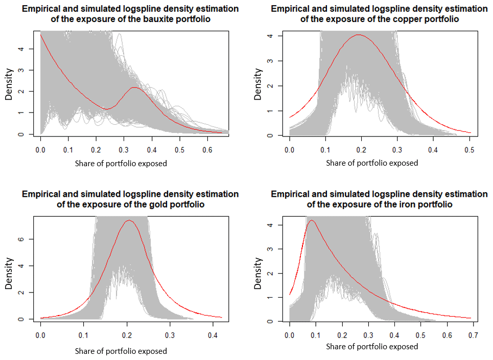
Figure 1 Empirical (red) and independent and identically distributed process-simulated (gray) density estimation of the yearly share of global production exposed to a wet or dry 10-year event according to the 12-month SPEI for four different portfolios.

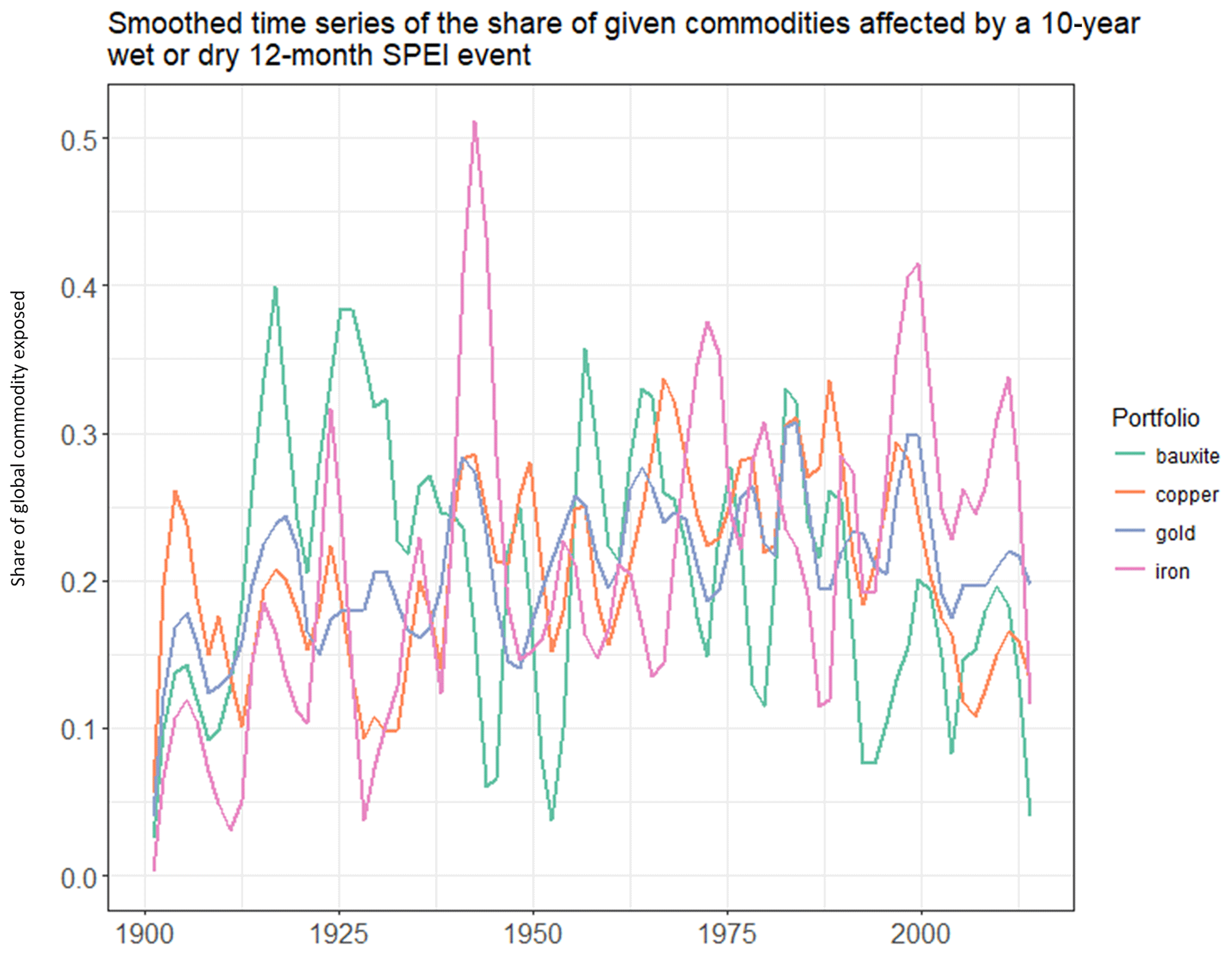
Figure 2 Time series of weighted global annual share of production exposed for different commodities with 11-year local regression-smoothed trends. Wet and dry events are considered.

In the worst year, nearly 40 % of the global land area experienced a 10-year dry or wet event. Sectoral impacts are heavily clustered when assets are concentrated in a few locations. This is for instance the case for phosphates, for which the worst year translated into a nearly 84 % exposure of global production, and for lithium and lead. Nearly 50 % of global copper production is exposed to a dry or wet event in the worst year of available data. For each of the portfolios considered, the worst exposure in the record has a negligible probability of occurrence if one were to consider the local 10-year return period events occurring independently and randomly over the earth. We assessed these probabilities using 100 000 simulations of the 114-year record assuming the same asset values at each mining site, as well as random sampling of hit or no hit independently at each location using the local marginal probabilities for the events. This illustrates that the spatial concentration of risk across the earth is dramatic for the tail events, highlighting the potential for multiple hits at the global scale a few years per century, much more frequently than may be expected by chance considering locations independent from each other. If, for a given commodity i, we call X_i the production exposed in a given year and M_i the maximum share of production exposed observed over 114 years, we have Table 1.

Table 1 Share of global commodity portfolios exposed to wet and dry events. M_i is the maximum share of production exposed observed over 114 years, and pexc(M_i) refers to the probability that this level of exposure or higher could occur across the different mining sites if the climate risks were not spatially correlated.

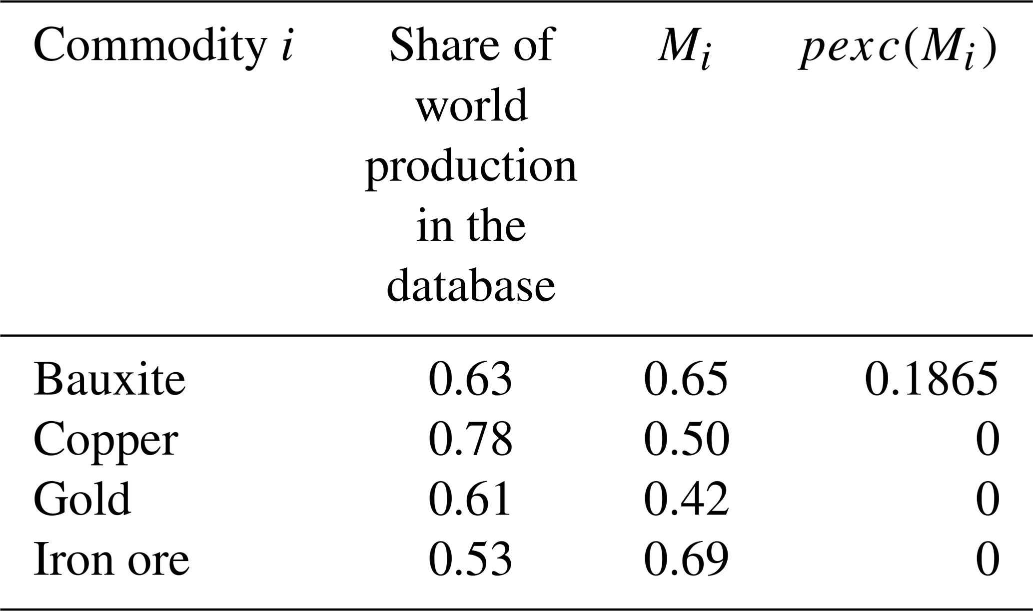
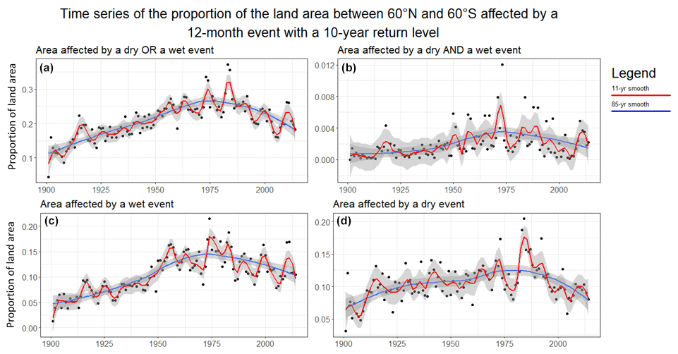
Figure 3 Proportion of global area affected annually by exceedance of the 10-year return level of the 12-month SPEI index for wet or dry (a), wet and dry (b), wet (c), and dry area (d) events with 95th confidence interval in shaded gray.

Density estimation (Fig. 1) also highlights the potential for fat tails, while smoothed time series of exposure with a smoothing window of 11 years (Fig. 2) make evident the existence of cycles.

Consistent with many analyses of longer duration hydrologic extremes (Greve et al., 2014; Sheffield and Wood, 2008; Sippel et al., 2017; Trenberth et al., 2014), the time series of global annual exposure for mining reveals a cyclical rather than monotonically increasing or decreasing trend (as may be expected from anthropogenic climate change). In several of the cases, using wavelet and spectral analyses we find evidence for connections to the El Niño–Southern Oscillation and to climate indices known to exhibit decadal variability (Figs. S9–S13).

Given these observations, we explored the global land area exposed. The temporal trend of the global land area exposed to the crossing of the dry and wet thresholds of the 12-month SPEI index is shown in Fig. 3. An increase in the area affected by events of all types occurred through the 1970s. This was followed by a decrease in the total affected area. Note that the threshold used to determine whether an extreme event occurred at a location or not is determined as the appropriate quantile at that location using the corresponding data source. Hence, generic biases in observations in the net water availability at any location are not an issue in determining whether or not an extreme event occurred.

The recent decrease in wet events is largely observed in the tropics and subtropics for the CRU data (Fig. S7). The 1982–1983 El Niño event corresponds to the highest number of extremes (Figs. 3 and 5). The 5 years that show up with the most events are (in decreasing order) 1983, 1984, 1973, 1974 and 1976. Except for 1984, these correspond to some of the strongest December–January–February (DJF) El Niño–Southern Oscillation (ENSO) conditions (El Niño for 1983 and 1973 and La Niña for 1974 and 1976) (NOAA ESRL, 2016). Wavelet analyses of the derived hit series (performed with biwavelet; Gouhier et al., 2016) show significant interannual and decadal variations and are coherent with the NINO3.4 index at interannual (4 years) and decadal (16 years) frequencies after 1970 (Fig. 4). Coherence is characterized by warmer colors, with significant regions circled in black. A multitaper spectral analysis (Rahim et al., 2017; Slepian, 1978; Thomson, 1982) also shows coherence for cycles of 4 years, consistent with the ENSO and North Atlantic Oscillation (NAO) phenomena (Fig. S14, where common oscillatory behaviors from multitaper analysis are marked by spikes with the x axes corresponding to cycles per year; thus a 0.2 value corresponds to a 5-year cycle) and with the Pacific Decadal Oscillation (PDO) index at scales of about 8 years.

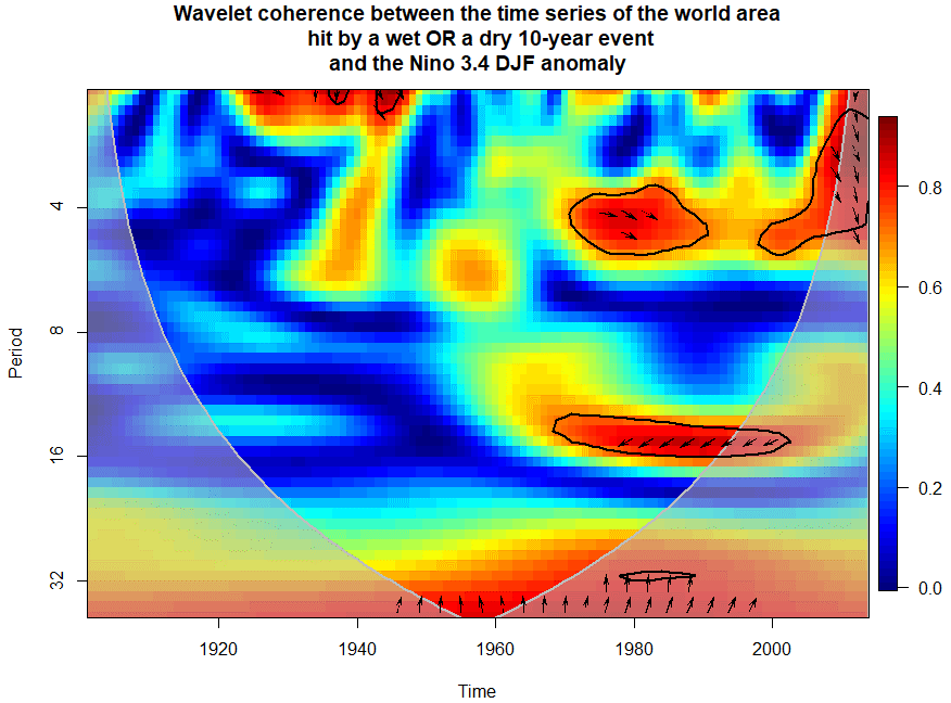
Figure 4 Wavelet coherence between the global share of area exposed and the Nino3.4 DJF anomaly. The arrow directions indicate the phase (0^∘ is concurrent, 180^∘ is perfectly out of phase) of the relationship between exposure and NINO3.4 for frequency bands and times when the coherence is statistically significant, as marked by the black encircled areas. The gray shaded zone indicates areas with edge effects that preclude a robust identification of significance given the combination of the sample size and the period of the oscillation.

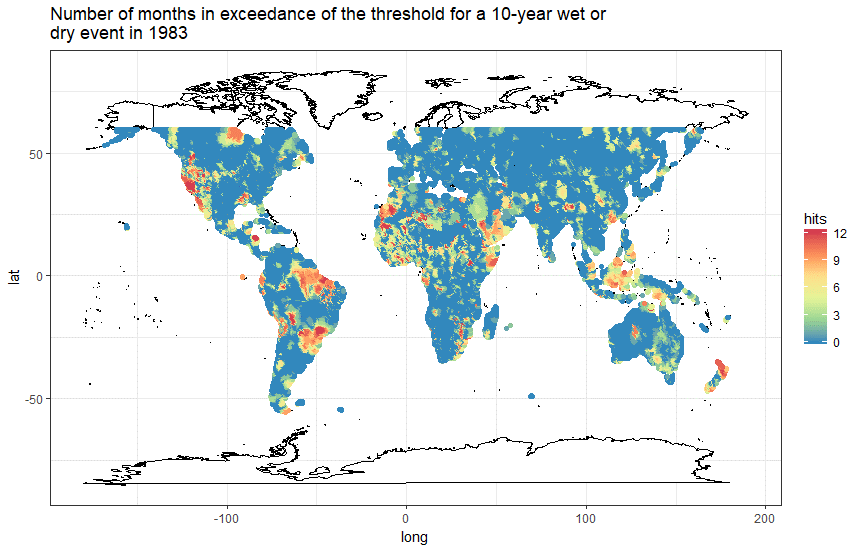
Figure 5 Map of the number of months in exceedance of a 10-year return level threshold for a wet or dry event in 1983. Here each month that exceeded either the wet or dry 10-year return level threshold counts as a “hit”.

The spatial teleconnections of hydrologic extremes to the El Niño–Southern Oscillation and other organized modes of interannual to decadal climate variability are well studied, and their impacts on agriculture and disasters are documented (Rojas et al., 2014). However, other than studies on the production of specific crops, an analysis of the impact of these climate modes on the aggregate global impact has not been previously done, especially considering a specific risk threshold.

4 Conclusion

In prior work (Bonnafous et al., 2017a, b) we illustrated impacts of hydrologic extremes with different return periods on mining company portfolios and the associated potential value at risk. For global companies and supply chains, the role of hydroclimatic risk clustering in space and time is not well studied, especially since the exposure could result from a combination of effects on real assets, transportation, energy, water and health infrastructure, production, and increase in local conflict under drought. A first step would be to develop influence diagrams that reflect the pathways of climate exposure for an investment portfolio or supply chain and then integrate social and economic factors to assess possible aggregate exposure. Critical path analyses on these exposure networks can then be performed to identify exposure pathways that contribute most significantly to the aggregate risk and to then develop risk mitigation strategies for those pathways. Such a framework would take into account compound events and simply “add” the space-time clustering of risk to a framework akin to the one advocated in Zscheischler et al. (2018). Examples of industry asset portfolios that could benefit from such analysis include (but are not limited to) renewable energy production facilities (e.g., dams for floods and droughts, windmills for extreme wind or low-wind periods) and transport infrastructure such as ports. Agriculture is a particular case, as much work has been done on it, and it would need to be properly integrated in the framework, for instance regarding the regional spatial extent and timing of droughts.

A question that arises once people understand the global portfolio-level risk due to the space-time correlation of exposure is how can someone who is exposed to such risk manage it? Examples of groups that could be exposed include (a) the World Food Program that provides food aid to regions that need it post-drought or post-flood for losses; (b) energy companies that are concerned with a disruption in the copper or lithium supply chain and associated shortages and price increases; and (c) multinational insurance companies faced with business interruption claims or correlated draws for payments. Parametric insurance and related financial instruments could provide an effective approach for risk mitigation in such cases. Examples of such products indexed to ENSO indices are available at scales ranging from farmer and micro-insurance to national banks to the World Food Program (Khalil et al., 2007; Carriquiry and Osgood, 2012; Hellmuth et al., 2009). Consider that a product were available where one could purchase a unit of insurance against a climate index (e.g., ENSO) exceeding a specified threshold, and the historical data for the index were publicly available. Then, a global or regional portfolio manager concerned with aggregate risk exposure could explore how often an exceedance of that threshold also led to an exceedance of the risk threshold for each element on their own exposure pathway and assess how well that index would influence their aggregate risk exposure. Where multiple climate indices are available for parametric insurance, the manager could optimize their allocation to a combination of those indices to mirror their risk exposure. Tradeoffs via reduction in exposure by considering alternate suppliers or by structural measures (e.g., storage or inventory) could also be considered.

Arguably, the SPEI provides a version of net precipitation and is advocated as a drought index. Indeed, for runoff, considerably more complex dynamics matter, but accurately modeling flooding risk at the asset scale globally is still confounded by considerable uncertainty.

Our intention here is to highlight the space-time clustering of the wet and dry risks for different sectors and not to model these effects at the asset scale. For this purpose, we considered the tail events of the long record of the SPEI to be useful. We did not consider the application of the state-of-the-art probabilistic drought and flood model at high spatial resolution globally to be necessary to make the same point. The uncertainty associated with the climatic and soil data and the lack of calibration and/or verification data from the application of such models may not justify the additional effort if the point to be made was one of the nature of space and time variation of climate and its implication for risk.

On the one hand, the quality of historical climate datasets degrades especially as one goes back before 1950. On the other hand, climate reanalysis products, as well as the Intergovernmental Panel on Climate Change (IPCC) climate model integrations for the 20th century, are known to show significant biases for hydroclimatic variables (Bozkurt et al., 2017; Ficklin et al., 2016; Liu et al., 2014). However, we expect the conclusion as to the space and time clustering that translates into a fat-tailed risk for global enterprises is robust.

On the other hand, one might advocate that the datasets used here may not fully represent extremes, especially on the wet side, as complex dynamics such as runoff conditions and hydrological routing are involved at the local level. However, accurately modeling flooding risk at the asset scale globally is still confounded by considerable uncertainty associated with the climatic and soil data and the lack of calibration and/or verification data from the application of state-of-the-art hydrological models. Plugging such a model into our approach is obviously feasible and could be part of a larger effort including exploring the risk-level space. Our goal was here to highlight that currently the space-time correlation structure of climate risk at the global scale due to quasi-periodic planetary-scale climate regimes is largely unaddressed by risk managers and to establish the need to do so, retrospectively and prospectively. Analyses of the biases and uncertainty attendant to future climate projections in this context are needed and will depend on the model and the space-time resolution of the analysis.