Analysis of meteorological parameters triggering rainfall-induced landslide: a review of 70 years in Valtellina

This paper presents an extended reanalysis of the rainfall-induced geo-hydrological events that have occurred in the last 70 years in the alpine area of the Lombardy region, Italy. The work is focused on the description of the major meteorological triggering factors that have caused diffuse episodes of shallow landslides and debris flow. The aim of this reanalysis was to try to evaluate their magnitude quantitatively.

The triggering factors were studied following two approaches. The first one started from the conventional analysis of the rainfall intensity (I) and duration (D) considering local rain gauge data and applying the I–D threshold methodology integrated with an estimation of the events' return period. We then extended this analysis and proposed a new index for the magnitude assessment (magnitude index, MI) based on frequency–magnitude theory. The MI was defined considering both the return period and the spatial extent of each rainfall episode.

The second approach is based on a regional-scale analysis of meteorological triggers. In particular, the strength of the extratropical cyclone (EC) structure associated with the precipitation events was assessed through the sea level pressure tendency (SLPT) meteorological index. The latter has been estimated from the Norwegian cyclone model (NCM) theory.

Both indexes have shown an agreement in ranking the event's magnitude (R²=0.88), giving a similar interpretation of the severity that was also found to be in accordance with the information reported in historical databases.

This back analysis of 70 years in Valtellina identifies the MI and the SLPT as good magnitude indicators of the event, confirming that a strong cause–effect relationship exists among the EC intensity and the local rainfall recorded on the ground. In respect of the conventional I–D threshold methodology, which is limited to a binary estimate of the likelihood of landslide occurrence, the evaluation of the MI and the SLPT indexes allows quantifying the magnitude of a rainfall episode capable of generating severe geo-hydrological hazards.

1 Introduction

In the context of geo-hydrological risk prevention, urban planners and infrastructure engineers still need instruments for carrying out trigger analysis (Ozturk et al., 2015; Papini et al., 2017; Piciullo et al., 2017). This is crucial to avoid human injures and material damage in those places where the natural landscape has been dramatically modified by uncontrolled urbanization (Albano et al., 2017b; Bronstert et al., 2018). Italy is a country historically affected by diffuse geo-hydrological fragility (Albano et al., 2017a; Ballio et al., 2010; Caine, 1980; Gao et al., 2018; Longoni et al., 2016). Alpine and Apennine mountain slopes represent the most vulnerable places of the country where shallow landslides and debris flow can occur more frequently (Ciccarese et al., 2020; Gariano and Guzzetti, 2016; Longoni et al., 2011; Montrasio, 2000; Montrasio and Valentino, 2016; Rossi et al., 2019; Vessia et al., 2014, 2016). We can cite several examples of past events such as the case of Valtellina (Lombardy) in 1987 as well as Piedmont in 1994 and 2000 and Genoa in 2011 and 2013 (ISPRA, 2018a). All of these catastrophic events have been caused by rather exceptional rainfall episodes that rarely occur and have particular features regarding their durations and their intensities (Ceriani et al., 1994; Corominas et al., 2014; Guzzetti et al., 2007; Rappelli, 2008). Here, the scientific literature has proposed some analytical methods for relating the triggering event to the occurrence of rainfall-induced landslides.

A first methodology consists of the analysis of the rainfall return period (RP) for establishing the intensity of the meteorological trigger (Caine, 1980; Iverson, 2000). The RP has a statistical meaning and represents the average recurrence time of a rainfall episode characterized by a certain intensity (I) and duration (D) that happened at a specified location (Bovolo and Bathurst, 2012; Frattini et al., 2009; Iida, 2004). This information can potentially be linked to the recurrence of the eventually triggered geo-hydrological phenomena in the case that we make the assumption of iso-frequency with the RP of precipitation (De Michele et al., 2005; ISPRA, 2018b). For a flood or a flash flood, that approximation is generally acceptable because an inundation represents the direct consequence of heavy precipitation (Albano et al., 2017a; De Michele et al., 2005). Instead, defining an RP for a landslide is not a common practice because the failure is not a periodic event but a sudden collapse (ISPRA, 2018b). For complex and deep-seated landslides the meteorological triggering factors are also intimately bounded with the local predisposing factors, i.e. the territory morphology, geology, etc. (Ciccarese et al., 2020; Guzzetti et al., 2007; ISPRA, 2018a; Longoni et al., 2016; Montrasio, 2000; Ozturk et al., 2015; Papini et al., 2017). The position of the surface rupture and the seasonal groundwater circulation can have a crucial interplay role influencing the overall stability of the landslide (Longoni et al., 2014; Ronchetti et al., 2009; Xiao et al., 2020). Therefore, it is not always clear how to identify the real cause of the collapse, and the correlation with rainfall triggers is sometimes weak (Ibsen and Casagli, 2004).

A certain degree of reciprocity with precipitation triggers is maintained mainly for rainfall-induced events such as shallow landslides, soil slips, and debris flows. Therefore, a common methodology consists of the investigation of rainfall intensity–duration (I–D) curves (Ceriani et al., 1994; Ciccarese et al., 2020; Crosta and Frattini, 2001; Gao et al., 2018; Guzzetti et al., 2008; Longoni et al., 2011; Olivares et al., 2014; Peruccacci et al., 2017; Rappelli, 2008; Rosi et al., 2016; Vessia et al., 2014, 2016; Segoni et al., 2014). The rainfall thresholds are valid for a specific region where in respect of the duration and the intensity of the precipitation episode a shallow terrain movement could be triggered or not triggered. These curves are created looking at the past events that occurred across a region; therefore, they are site-specific (Ceriani et al., 1994; Guzzetti et al., 2008; Rappelli, 2008; Rossi et al., 2012). Intrinsically they include the susceptibility of the local territory to landslide failure, so their use cannot always be extended to other regions with different geological and morphological characteristics (Caine, 1980; Guzzetti et al., 2007; ISPRA, 2018b; Longoni et al., 2011; Peruccacci et al., 2017; Ozturk et al., 2018). Moreover, due to their empirical nature, I–D curves are sometimes rather approximate and could detect “false alarms” or, conversely, miss some “true alarms” (Abbate et al., 2019; Guzzetti et al., 2007; Peres et al., 2018). Some studies have demonstrated their dependency on the humidity condition of superficial terrain (Jie et al., 2016; Lazzari et al., 2018). This characteristic adds further uncertainties to the reliability of the I–D method. However, the I–D thresholds are widely used in the field of geo-hydrological risk prevention because they permit the giving of a fast preliminary prediction of the occurrence of shallow soil failures as part of local meteorological predictions (Piciullo et al., 2017).

Through the I–D threshold methodology, it is possible to distinguish critical events from non-critical ones, but no further information can be retrieved directly about their magnitude. One possible solution is to try to integrate rainfall thresholds with the probability of temporal occurrence considering again the RP of the rainfall events, under the assumption of iso-frequency between the triggers and the geo-hydrological effects: low-magnitude events exhibit higher probabilities of occurrence, while greater-magnitude episodes have rare frequencies. In addition, I–D points that exhibit higher RPs are generally located at a higher distance from the I–D thresholds (Crosta and Frattini, 2001). This fact is explained by recalling the statistic of the precipitation extremes (De Michele et al., 2005) where, for any fixed rainfall duration, the increase in rainfall intensity determines an increase in the RP. For these reasons, that “point–threshold” distance is related to the RP and in principle could be considered for a magnitude classification of the critical event identified. Unfortunately, this assumption is generally valid only for events recorded around a very limited area where precipitation statistics are supposed to be spatially invariant.

Up to this point, we have presented the most common strategies adopted for describing the precipitation characteristics in rainfall-induced geo-hydrological events. In these methodologies only I and D parameters are investigated, but are these methods enough for a complete description of the rainfall triggering factors? Is the RP a good predictor of their magnitude? Can rainfall analysis be improved also considering other meteorological variables that are related to the magnitude of the trigger? In our study, we have tried to answer these questions by proposing an alternative to the conventional I–D rainfall analysis which is able to classify rainfall events according to the spatial extent of their impact. We propose a reanalysis of past meteorological events which provoked several landslide events. We have investigated rainfall triggers not only considering local rain gauge time series but also including a broader description of the events looking at meteorological reanalysis maps at a regional scale. The goal was to establish a magnitude ranking among the rainfall-induced geo-hydrological events studied in order to identify the most critical ones. In this light, a 70-year reanalysis study is presented starting from a group of past rainfall episodes that happened in the alpine region of northern Lombardy, Sondrio Province, Italy (Sistema Informativo sulle Catastrofi idrogeologiche, 2020; Rappelli, 2008; Tropeano, 1997). Triggering factors are interpreted following two approaches:

• In the first approach, we put the events in the context of the classical I–D approach, integrated with the estimation of the RP, as mentioned earlier. We then propose an alternative for the classification of the events' magnitude through the introduction of a magnitude index (MI). The index incorporates the return period of an event with the spatial extent of its impact in terms of landslide occurrence. The MI is defined as a substitution for the classical magnitude quantification adopted for geo-hydrological events (Corominas et al., 2014; Malamud et al., 2004).

• A second approach is based on a meteorological analysis of the triggers, considering their interpretation via the Norwegian cyclone model (NCM) (Godson, 1948; Martin, 2006; Stull, 2017). Here, the trigger's magnitude is expressed through a physically based meteorological index called the sea level pressure tendency (SLPT) which is a function of some atmospheric parameters evaluated at the synoptic scale and associated with the rainfall event.

To carry out our study two data sources are considered:

• ground-based meteorological series of rainfall events (ARPA Lombardia, 2020; SCIA, 2020), adopted for the I–D methodology and for the RP evaluation;

• meteorological maps provided by the National Centers for Environmental Prediction (NCEP) (Kalnay et al., 1996; MeteoCiel, 2020) for the NCM intensity assessment.

The paper will be organized as follows: in Sect. 2 a brief description of the historical databases and the meteorological reanalysis maps is presented; in Sect. 3 the two methodologies behind the definition of the MI, through the extended rain-series analysis, and the SLPT, through the NCM theory, are described; in Sect. 4 the outcomes from the two presented approaches are reported and the two indexes are then compared. A discussion is developed in Sect. 5 with some comments about the obtained results, with a focus on the SLPT index performances; in the last section some final remarks and conclusions about the ongoing research work are reported.

2 Data and materials

2.1 Historical database of geo-hydrological events and rainfall time series

A group of past geo-hydrological events has been considered from the alpine area of Sondrio Province, northern Lombardy, Italy (Fig. 1). In our study, we have investigated historical databases to identify events that in the recent past exhibited similar cause–effect behaviour, like the 1987 event. In July 1987 this area was affected by exceptional geo-hydrological events triggered by a rather intense and prolonged rainfall episode (Rappelli, 2008; Tropeano, 1997). The effects on the territory were severe: shallow landslides, debris flows, and flash floods were recorded causing human injuries; 35 fatalities; and extensive damage to infrastructure and buildings, estimated at EUR 2 billion (Sistema Informativo sulle Catastrofi idrogeologiche, 2020).

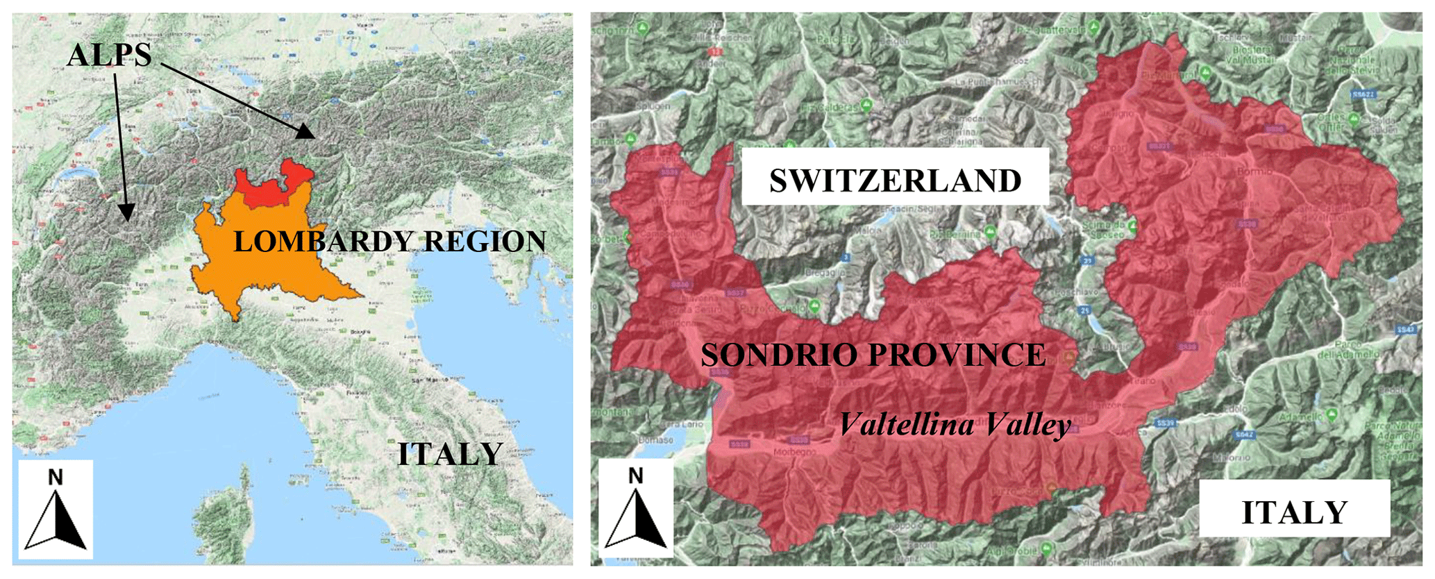
Figure 1 Case study area of Sondrio Province, northern Lombardy; base layer from © Google Maps 2020.

Two different data sources were investigated to collect historical data: the Aree Vulnerate Italiane (AVI) database and the Inventario Fenomeni Franosi Italiano (IFFI) database (Sistema Informativo sulle Catastrofi idrogeologiche, 2020). The data collect historical information from past natural disasters from the medieval age up to nowadays; the AVI database is directly available via a geoportal website (http://sici.irpi.cnr.it/; last access: July 2021) that is managed by CNR (Consiglio Nazionale delle Ricerche), and the IFFI database is available from a national geoportal website (Sistema Informativo sulle Catastrofi idrogeologiche, 2020). Available event time series were not homogeneous, so the consistency of the database was evaluated, redundant records have been dropped, and final integration between the AVI and the IFFI database information was carried out.

The period chosen for the reanalysis is between 1951 and 2019. Systematic monitoring of the precipitation and temperature was started in Italy in 1951 by SIMN (Servizio Idrografico e Mareografico Nazionale), and looking at the antecedent periods these data were missed or characterized by several uncertainties or errors (SCIA, 2020). The available rain gauge data series were gathered from local archives of SIMN (SCIA, 2020) and ARPA Lombardia (ARPA Lombardia, 2020). These series were conventionally recorded on a daily basis until the 2000s, so “daily rain” represents the maximum resolution of our dataset before that period. Starting from 2001, the available temporal resolution has moved to a sub-hourly time step, increasing the accuracy of the rainfall analysis.

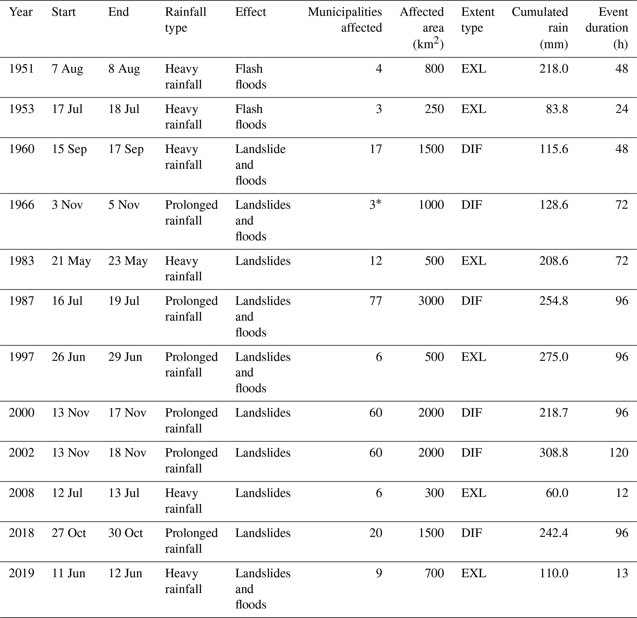
In the AVI and IFFI databases, the precise location of geo-hydrological episodes was not available even for the most recent events that happened after the 2000s. Therefore, some indications about locations were retrieved from the AVI database considering the municipalities affected by disasters. The spatial extent of affected areas (AAs) describes those locations that have experienced some damage due to geo-hydrological events that have occurred. This information is indicative of the area where the rainfall event has been supposed to be more intense. In fact, AA was then compared with ground-based rain gauge series from the entire Sondrio Province with the aim to reconstruct for each rainfall event its spatial distribution. Selected events have been classified in terms of the AA parameter: extremely localized events (EXLs), with an influence area lower than 1000 km², or diffuse events (DIFs), with significant territorial diffusion greater than 1000 km². This threshold has been motivated referring to the nature of the meteorological triggers: EXLs were generally associated with convective rainfall phenomena whose extent is of the order of 10×10 km², and DIFs were characterized by diffuse and uniform rainfall with an extent of around 100×100 km² (Martin, 2006; Rotunno and Houze, 2007). In Table 1 a list of geo-hydrological events analysed in our study is reported.

2.2 NCEP reanalysis maps

To improve the description of rainfall triggering factors, the meteorological reanalysis maps were examined considering the National Centre for Environmental Prediction (NCEP) data (Kalnay et al., 1996; MeteoCiel, 2020; NOAA, 2021). The latter has a spatial resolution of $\mathrm{2.5}{}^{\circ }\times \mathrm{2.5}{}^{\circ }$ latitude by longitude, covering the whole planet with a temporal frequency of 12 h. All the data stored in NCEP maps are useful for the interpretation of air mass dynamics in the middle latitudes such as the extratropical cyclones (ECs) that are responsible for the spatial and temporal evolution of intense precipitation phenomena. For the European region, ECs develop in the Atlantic Ocean near the British Isles. ECs are responsible for a large part of the precipitation recorded over the Alps mountain range (Rotunno and Houze, 2007) because they are generally advected eastward through the Mediterranean area by Rossby waves (RWs) (Grazzini and Vitart, 2015; Martin, 2006). At the boundary of the polar vortex, RWs can generate strong jet streams that can move air masses in the direction of the Southern Alps, enhancing vertical air motions. Across the southern flank of the Alps, this mechanism may trigger persistent and heavy precipitation (Rotunno and Houze, 2007) that can intensify if an orographic uplift of the incoming southerly flow is also triggered (Abbate et al., 2021; Grazzini, 2007). Rainfall can reach remarkably high amounts if these conditions are prolonged for several days, leading to up to 400 mm in 2 to 3 d (Grazzini, 2007; Rotunno and Houze, 2007). For each event listed in Table 1, we have examined correspondent NCEP maps to investigate the mechanism responsible for generating such intense precipitation over the target area.

3 Model and methods

The trigger analysis is presented here considering the I–D thresholds approach, its extension through the MI definition, and the NCM with SLPT index evaluation.

3.1 Rainfall I–D thresholds and return period analysis

The daily rainfall rate has been determined from the total amounts and the duration listed in Table 1. Rainfall amount (RA) was estimated keeping the distinction between EXLs and DIFs (Fig. 2a). For EXLs the nearest rain gauge or the two nearest rain gauges were chosen as reference. For DIFs, all the available daily rain data RA_i in the territory have been summed and averaged considering the number of rain gauge stations n to obtain a representative value for RA_avg (Eq. 1a). We have assumed a uniform spatial distribution of the rain gauge stations, Fig. 2b, neglecting any influence of elevation on rainfall data (Abbate et al., 2021). Then, the rainfall rate (RR) was computed as the ratio of the cumulative rainfall RA_avg to the duration D (Eq. 1b).

$$\begin{array}{}\text{(1a)}& {\displaystyle }& {\displaystyle }{\mathrm{RA}}_{\mathrm{avg}}={\displaystyle \frac{\sum _{i=\mathrm{1}}^n{\mathrm{RA}}_i}{n}}\mathrm{in}\mathrm{mm}\text{(1b)}& {\displaystyle }& {\displaystyle }\mathrm{RR}={\displaystyle \frac{{\mathrm{RA}}_{\mathrm{avg}}}{D}}\mathrm{in}\mathrm{mm}{\mathrm{h}}^{-\mathrm{1}}\end{array}$$

Figure 2 (a) Distribution of critical events across Sondrio Province and (b) the local rain gauge station network considered in the study; base layer from © Google Maps 2020.

Table 1 Geo-hydrological events recorded from 1951 up to 2019 considered for the back-analysis study. In the table the event classification is also reported considering the events' spatial extent: the extreme localized events (EXLs) and the more diffuse ones (DIFs). ^* indicates uncertain data.

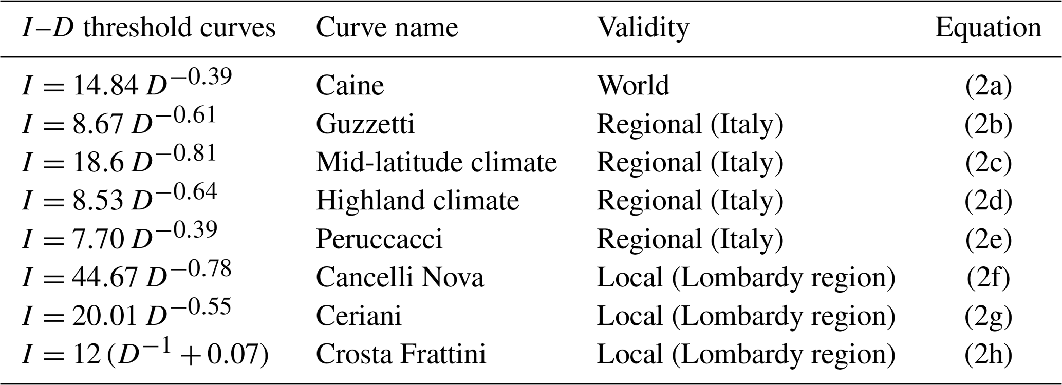
For the studied area, a set of thresholds proposed in the literature was considered, reported in Table 2. All the rainfall thresholds have a monomial expression, where D is the duration of the rainfall (hours), and I is the average rainfall intensity (mm h⁻¹). The “Caine” curve (Eq. 2a) (Caine, 1980) is the most general one, valid worldwide for shallow landslides and debris flow phenomena. At a regional scale, a more recent study conducted by Guzzetti et al. (2007) proposed a new set of curves valid for central and southern Europe, considering a distinction among different climate types. In our study, three of them were selected: the general one (“Guzzetti” curve; Eq. 2b), the curve valid for mid-latitude climate (“mid-latitude climate” curve; Eq. 2c), and the one suitable for highlands and mountain environments (“highland climate” curve; Eq. 2d). Another study from Peruccacci et al. (2017) further extended the previous study by Guzzetti et al. (2007), addressing a new I–D threshold (“Peruccacci” curve) valid for the Italian country. At the local scale, the “Cancelli Nova” (Eq. 2e) (Rappelli, 2008), the “Ceriani” (Eq. 2f) (Ceriani et al., 1994), and the “Crosta Frattini” curves (Eq. 2h) (Crosta and Frattini, 2001) were proposed in 1985, 1994, and 1998 respectively. All of them were calibrated directly on the recorded data available in Sondrio Province.

Table 2 I–D threshold curve set considered in this study.

For each event, the coupled points RR–D were plotted against the I–D threshold curves, and their return period (RP) was evaluated. The latter was determined following the methodology based on the IDF (intensity–duration–frequency) curves (De Michele et al., 2005) available for the Lombardy region and provided by ARPA Lombardia (2020). The coefficients of IDF curves are estimated through the analysis of rainfall extremes addressing the GEV (generalized extreme value) distribution. The dataset considered for the GEV was the SIMN time series (SCIA, 2020) gathered from 1960 up to 1990 across the whole territory of the region. Bearing in mind that our localized events (EXLs) have been distinguished from the diffuse events (DIFs), including for the RP calculation, we have considered the same assumptions as for RR evaluation. For the localized events, the on-site coefficient of IDFs has been taken, while for the diffusive ones, a spatially averaged value has been computed.

3.2 Trigger hazard estimation and the magnitude index (MI)

A further step in the precipitation analysis consists of the hazard and magnitude assessment for each event. According to Guzzetti et al. (2005) the general landslide hazard could be defined as a probabilistic function of three terms (Eq. 2a): the size A_l, the temporal occurrence T_l, and the spatial susceptibility S. The “size” term stores the information about the volume, the area, or the density of landslides that have occurred over a particular area. The temporal occurrence considers the periodical reactivation of a single landslide (deep-seated) or the recurrence of shallow landslides inside a catchment. The spatial susceptibility represents the quantification of the territory predisposition to a landslide phenomenon.

$$\begin{array}{}\text{(2a)}& {\displaystyle }& {\displaystyle }{H}_{\mathrm{landslide}}=P\left(A_{\mathrm{l}}\ge a_{\mathrm{l}}\right)\cdot P\left(T_{\mathrm{l}}\ge t_{\mathrm{l}}\right)\cdot S\text{(2b)}& {\displaystyle }& {\displaystyle }S=\mathrm{1}\text{(2c)}& {\displaystyle }& {\displaystyle }\log \left(P\left(A_{\mathrm{l}}\ge a_{\mathrm{l}}\right)\right)=a-b\mathrm{AA},\mathrm{where}a\mathrm{and}b\mathrm{are}\mathrm{the}\mathrm{coefficients}\text{(2d)}& {\displaystyle }& {\displaystyle }\log \left(P\left(T_{\mathrm{l}}\ge t_{\mathrm{l}}\right)\right)=c-d\mathrm{RP},\mathrm{where}c\mathrm{and}d\mathrm{are}\mathrm{the}\mathrm{coefficients}\end{array}$$

Starting from the definition of Eq. (2a), we have extended this concept and adapted it to interpret the events in our reanalysis study. The aim was to define a proper hazard and then a magnitude indicator for geo-hydrological events considering the temporal and spatial probability of occurrence of the triggering rainfall. According to Malamud et al. (2004) a scale for the magnitude is necessary to interpret quantitatively the episodes and to highlight the most severe ones. For landslides and rainfall-induced geo-hydrological events, a unique method that describes the “energy” does not exist because several variables may play an important role in its definition (Bovolo and Bathurst, 2011; Frattini et al., 2009; Gao et al., 2018; Iida, 2004; Reid and Page, 2003). Therefore, making some assumptions, we have proposed a new magnitude index (MI) as a quantitative parameter for assessing a proper magnitude ranking. Firstly, we have assumed that the investigated area had a homogeneous susceptibility S=1 to shallow landslides and debris flow triggering. This choice was motivated by geological and morphological features and also by looking at recent susceptibility maps proposed by ISPRA (2018b). Then we moved to other terms trying to determine the spatial and temporal probability of exceedance from AA and RP parameters, recalling the theory of the frequency–magnitude relationship.

The frequency–magnitude curve (FMC) was proposed by Gutenberg and Richter (1944) for earthquake studies and then was also extended for interpreting different types of natural phenomena (Gao et al., 2019). The MCF curve is obtained by plotting incremental frequency F_i against the magnitude M_i on a logarithmic scale. F_i represents the frequency of the event that has a magnitude greater than or equal to a certain value M_i. In our study, the MFCs were considered to evaluate the probability of occurrence of a certain event in time and space and then combined to determine its hazard as described in Eq. (2a). The temporal occurrence term requires the estimation P(T_l≥t_l) from the RP's frequency–magnitude relationship. This represents the probability of occurrence of an event T_l with RP ≥t_l. According to Guzzetti et al. (2005), the other hazard component is addressed by the landslide size (Eq. 2d). In this regard, in our database it was not possible to retrieve enough information about event features, such as the volumes and areas involved or the numbers of landslide failures. Therefore, the AA parameter was used as a proxy for the “trigger's size” and was treated similarly to the RP term. The probability of spatial occurrence P(A_l≥a_l) of an event A_l with AA ≥ a_l was retrieved from the FMC (Eq. 2c). Then, the hazard was estimated using Eq. (3a). Due to the modification of the first term P(A_l≥a_l), it does not properly represent the landslide hazard, but H_trigger is an indicator of the hazard as a function of the trigger's temporal frequency and spatial extent.

In most natural cases, the frequency of low-magnitude geo-hydrological events is rather high and vice versa. Therefore, we tried to estimate the trigger magnitude as an inverse function of the hazard. The latter is a combination of two probabilities of occurrence (Eq. 3b); therefore it can be transformed into a magnitude recalling again the FMC in Eq. (3c). Working out some algebra with Eq. (3a–c) we have obtained a representation of the magnitude expressed by the MI (Eq. 3d). The MI is a sum of two contributions: the first describes its spatial extent through the parameter AA, and the second describes its temporal occurrence through the RP. In this light, the MI was intended to be more complete rather than the single RP because through the AA term it is possible to consider the “integral effects” related to the trigger's extent. The MI was taken as a reference for testing the SLPT index presented in the next section.

$$\begin{array}{ll}\text{(3a)}& {\displaystyle }& {\displaystyle }{H}_{\mathrm{trigger}}=P\left(A_{\mathrm{l}}\ge a_{\mathrm{l}}\right)\cdot P\left(T_{\mathrm{l}}\ge t_{\mathrm{l}}\right)\text{(3b)}& {\displaystyle }& {\displaystyle }{H}_{\mathrm{trigger}}=\exp (a-b\mathrm{AA})\cdot \exp (c-d\mathrm{RP}){\displaystyle }& {\displaystyle }{M}_{\mathrm{trigger}}=-\log \left(H_{\mathrm{trigger}}\right)=-\log \left(\exp \right(a-b\mathrm{AA})\\ \text{(3c)}& {\displaystyle }& {\displaystyle }\cdot \exp (c-d\mathrm{RP}))\text{(3d)}& {\displaystyle }& {\displaystyle }\mathrm{MI}=M_{\mathrm{trigger}}=-\left(\right(a-b\mathrm{AA})+(c-d\mathrm{RP}\left)\right)\end{array}$$

3.3 NCM and SLPT index

The extratropical cyclone dynamic influences the rainfall intensities: if the EC is stronger, more precipitation is expected over an area, but, depending on EC spatial and temporal evolution, rainfall could exhibit different total amounts and durations. Therefore, using the NCEP maps, the Norwegian cyclone model (NCM) (Godson, 1948; Martin, 2006; Stull, 2017) was chosen for estimating a strength index of ECs. The NCM was formulated in the early 20th century. It describes an extratropical cyclone that develops as a disturbance along the boundary (front) between the polar and mid-latitude air masses. The model calculates indirectly the sea level pressure tendency (SLPT), the time $/$ variation ratio of sea level atmospheric pressure $\mathrm{\Delta }{p}_{\mathrm{sl}}/\mathrm{\Delta }t$ (hPa h⁻¹) that represents an indicator of the strength of a cyclone structure (Andrews, 2010; Godson, 1948; Martin, 2006; Stull, 2017; Wallace and Hobbs, 2006). When the EC is more intense, the absolute value of the SLPT ratio is higher, and, consequently, the EC can cause more rainfall. According to Stull (2017), this index is obtained as a sum of four different influencing factors that correspond to the processes implicated in the dynamic evolution of extratropical cyclones:

$$\begin{array}{}\text{(4)}& {\displaystyle \frac{\mathrm{\Delta }{p}_{\mathrm{sl}}}{\mathrm{\Delta }t}}=T_{\mathrm{1}}+T_{\mathrm{2}}+T_{\mathrm{3}}+T_{\mathrm{4}}=\mathrm{SLPT}.\end{array}$$

• T₁ expresses the “upper-layer divergence mechanism” due to jet streams, which removes air mass from the air column. In Eq. (5b), ρ_MID=0.5 kg m⁻³ is the average density of air column and g is 9.8 m s⁻². W_MID (m s⁻¹) is the mean air column vertical velocity that is evaluated considering Eq. (5a) in the proximity of the local change in the jet stream velocity gradient ΔW_js (m s⁻¹), where Δz is approximately equal to 5000 m and Δs₁ (m) is jet streak elongation. According to Stull (2017), Eq. (5a) is a strong approximation because it supposes air density to be constant over the air column, so we have considered a revised version (Stull, 2017) that expresses the W_MID in terms of other parameters such as the geostrophic wind velocity G (m s⁻¹), the curvature radius R (km) of Rossby waves, and the Coriolis parameter f_c (s⁻¹);

  $$\begin{array}{}\text{(5a)}& {\displaystyle }{W}_{\mathrm{MID}}={\displaystyle \frac{\mathrm{\Delta }{W}_{\mathrm{js}}}{\mathrm{\Delta }z/\mathrm{\Delta }{s}_{\mathrm{1}}}},\text{(5b)}& {\displaystyle }{T}_{\mathrm{1}}=-g{\mathit{\rho }}_{\mathrm{MID}}{W}_{\mathrm{MID}}.\end{array}$$

• T₂ is the “atmosphere boundary layer pumping”, which causes the horizontal wind to spiral inward toward a low-pressure centre. In Eq. (6b), the air density of the boundary layer is ρ_BL=1.112 kg m⁻³. W_BL (m s⁻¹) comprises the vertical velocities at the boundary layer calculated through Eq. (6a) following the approach proposed by Stull (2017) for cyclone structures; the b_BL factor is a function of boundary layer thickness that can be assumed equal to 1000 m on average, and the drag coefficient C_d≈0.005 is defined for flow over land;

  $$\begin{array}{}\text{(6a)}& {\displaystyle }{W}_{\mathrm{BL}}={\displaystyle \frac{\mathrm{2}{b}_{\mathrm{BL}}{C}_{\mathrm{d}}}{f_{\mathrm{c}}}}{\displaystyle \frac{G^{\mathrm{2}}}{\mathrm{\Delta }{s}_{\mathrm{2}}}},\text{(6b)}& {\displaystyle }{T}_{\mathrm{2}}=g{\mathit{\rho }}_{\mathrm{BL}}{W}_{\mathrm{BL}}.\end{array}$$

• T₃ expresses the horizontal air mass advection that moves a low-pressure centre in the direction of the target region (Eq. 7b). The advection velocity M_c (m s⁻¹) is a function of the celerity of Rossby waves c_RW (m s⁻¹) and the geostrophic wind G (Eq. 7a). The spatial pressure gradient at sea level is evaluated considering the distance Δs₂ (m) between the low-pressure centre and the target region;

  $$\begin{array}{}\text{(7a)}& {\displaystyle }{M}_{\mathrm{c}}=c_{\mathrm{RW}}-G,\text{(7b)}& {\displaystyle }{T}_{\mathrm{3}}=-M_{\mathrm{c}}{\displaystyle \frac{\mathrm{\Delta }{p}_{\mathrm{GW}}}{\mathrm{\Delta }{s}_{\mathrm{2}}}}.\end{array}$$

• T₄ is the “latent heating” due to water vapour condensation in rainfall. It comes from the theory of thermodynamic transformations of water vapour in the atmosphere where all the parameters for rain condensation processes are stored in the term b_AD. The precipitation that does reach the ground is related to the net amount of condensational heating during the time interval Δt of Eq. (8a) where T_v (K) is average air column virtual temperature, a is 10⁻⁶ km mm⁻¹, Δz (km) is the depth of the air column, the ratio of latent heat of vaporization to the specific heat of air is $L_{\mathrm{v}}/C_{\mathrm{p}}=\mathrm{2500}$ K per kilogram of air per kilogram of liquid and ρ_air and ρ_liq are air and liquid-water densities respectively, with ρ_liq=1000 kg m⁻³. The hypsometric equation relates to pressure–temperature changes as reported in Eq. (8b). For an air column with an average virtual temperature of T_v≈300 K, we obtain b_AD=0.082 kPa mm⁻¹ in Eq. (8c) which is considered for the description of the net column-average effect.

  $$\begin{array}{}\text{(8a)}& {\displaystyle \frac{\mathrm{\Delta }{T}_{\mathrm{v}}}{\mathrm{\Delta }t}}={\displaystyle \frac{a}{\mathrm{\Delta }z}}{\displaystyle \frac{L_{\mathrm{v}}}{C_{\mathrm{p}}}}{\displaystyle \frac{{\mathit{\rho }}_{\mathrm{liq}}}{{\mathit{\rho }}_{\mathrm{air}}}}\mathrm{RR}\text{(8b)}& {\displaystyle \frac{\mathrm{\Delta }{P}_{\mathrm{s}}}{\mathrm{\Delta }t}}=-{\displaystyle \frac{g}{T_{\mathrm{v}}}}{\displaystyle \frac{L_{\mathrm{v}}}{C_{\mathrm{p}}}}{\mathit{\rho }}_{\mathrm{liq}}\mathrm{RR}=-b_{\mathrm{AD}}\mathrm{RR}\text{(8c)}& {\displaystyle }{T}_{\mathrm{4}}=-b_{\mathrm{AD}}\mathrm{RR}\end{array}$$

When the balance in Eq. (4) is negative, cyclogenesis occurs. T₁, T₃, and T₄ bring a negative contribution to strengthening the EC cyclogenesis and lowering the SLPT index. In contrast, T₂ has a positive contribution and tends to weaken the EC structure, increasing the SLPT value. In Fig. 3a and b the mechanisms described by four terms (T_i) are depicted. Figure 3c reports how the model works considering the contribution of each four components across the timeline (A to G) that represents the stages of EC: the EC's formation phase (i.e. cyclogenesis) is from stages A to D, and the EC's dissipation phase (i.e. cyclolysis) is from D to G. The critical phase of the EC is in the proximity of point D where negative terms overcome the positive one. The SLPT index has been evaluated in connection to the C and D stages.

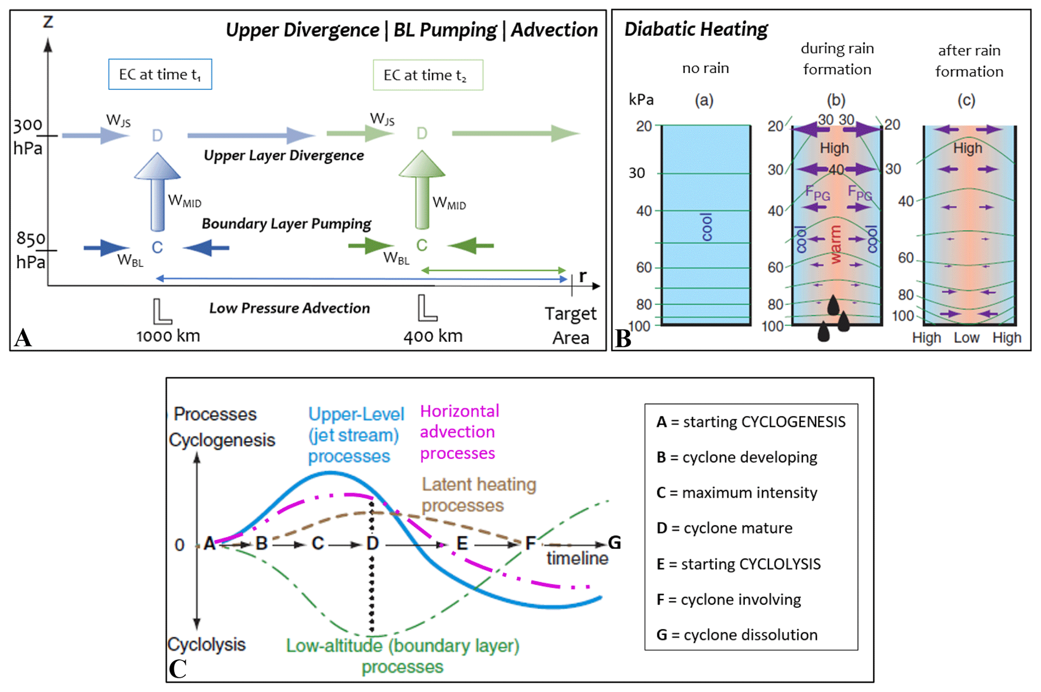
Figure 3 (a) Scheme of the mechanism represented by the T₁, T₂, and T₃ terms; (b) scheme of the mechanism represented by the T₄ term; (c) qualitative temporal evolution of each of the four terms T₁, T₂, T₃, and T₄ during cyclone phases (A to G) and their contribution to cyclone formation (cyclogenesis) and cyclone dissolution (cyclolysis), modified after Stull (2017).

4 Results

In this section, the results are presented in four steps. Firstly, the qualitative analysis coming from the direct interpretation of the database and NCEP maps is reported. Secondly, the I–D rainfall analysis is carried out and the MI evaluation is described. Thirdly, for each considered event, the SLPT is estimated and then compared with the MI.

4.1 Database interpretation and NCEP maps

The dataset of Table 1 shows a clear seasonal distribution of the events mainly concentrated during the summer and autumn seasons. July and November are the months more prone to geo-hydrological events, and this strong seasonality highlights that the trigger phenomena involved may have different origins (Martin, 2006; Rotunno and Houze, 2007). In July, meteorological events are characterized mainly by high intensity and short duration with a typical convective behaviour of precipitation (thunderstorms), and their average duration is generally around 1 or 2 d. In particular, 1951, 1953, 1987, 1997, 2008, and 2019 events happened during the summer season, and cumulated rainfall comprised between 100–200 mm, apart from in 1987 and 1997 which were rather exceptional (254 and 275 mm in 3 d). During October and November, rainfall events are characterized by higher persistency (4–5 d) and cumulated rainfall can easily reach amounts around 250–350 mm, such as for the events that happened in 2000, 2002, and 2018.

Through the analysis of NCEP maps, we have observed that all the events reported in Table 1 have been triggered in connection with EC structures that moved eastward from the Atlantic Ocean in the direction of the Alpine mountain range. In Fig. 4 three examples of reanalysis maps are reported that show the pressure distribution at a 500 hPa reference height across Europe during the 1966, 2002, and 2018 events. A qualitative comparison among the three maps highlights that three events have been characterized by the evolution of a rather intense EC that is recognizable from the deep low pressure (L) located near the British Isles. This recurrent configuration has been responsible for the torrential rainfall recorded in the Southern Alps across Sondrio Province. Consequently, the geo-hydrological effects could be directly attributed to the intensification of these EC structures. Starting from this qualitative evidence we have moved to a quantitative analysis following the two approaches proposed.

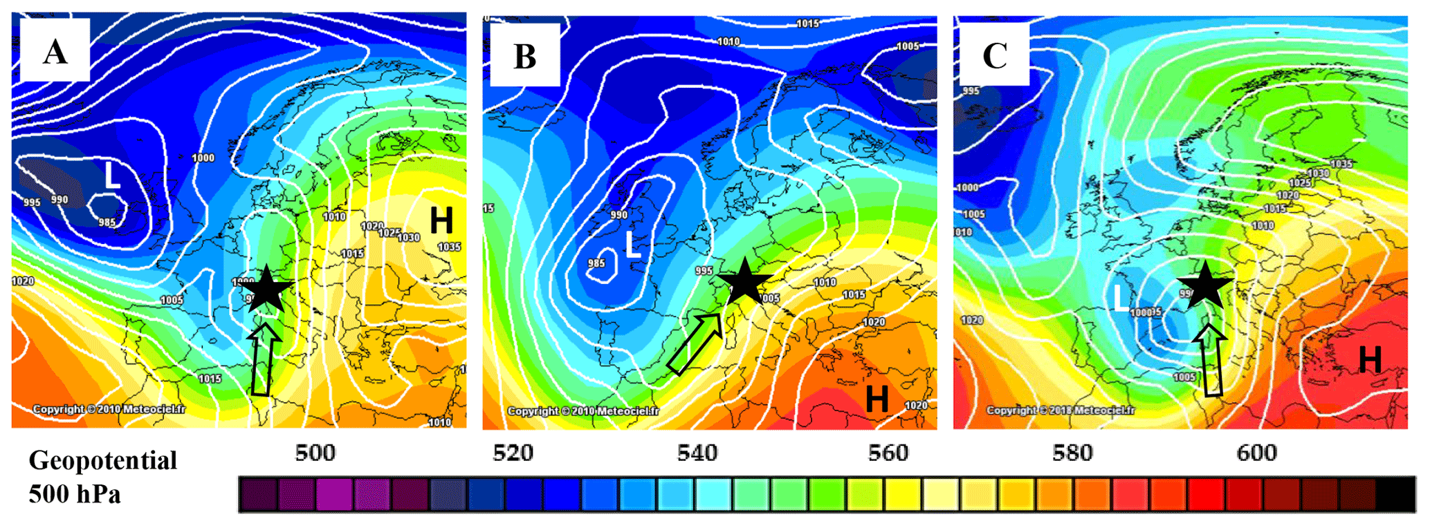
Figure 4 Reanalysis maps from NCEP reporting the sea level pressure and 500 hPa pressure (colours) for the 1966 (a), 2002 (b), and 2018 (c) events, where the black star is the Sondrio Province position and the black-outlined arrow indicates the incoming southerly flow responsible for huge precipitation enhancement, adapted from © MeteoCiel (2020).

4.2 Approach 1 – I–D threshold rainfall analysis and MI extension

In Fig. 5, the average daily rain rate I and the duration D of the rainfall episodes in Table 1 were plotted against the rainfall threshold curves listed from Eq. (2a–f). Most events can be clustered in the bottom right corner of the graph due to their characteristics of a rather long duration of 2–4 d and slightly low intensities. Only the events of 2019, 2008, and 1953 are dispersed on the other side of the graph where the duration is around or less than 1 d.

Figure 5 Intensity–duration thresholds for considered events and the relative rainfall RP.

Considering the thresholds proposed by Guzzetti et al. (2007), all the events are correctly identified above these curves (Fig. 5). No significant differences are seen between the general one (b), the curve valid for mid-latitude climate (c), and the one valid for highland climate (d). Peruccacci (e) and Crosta Frattini (h) are positioned intermediately between the regional threshold of Guzzetti and the local ones of Cancelli Nova (f) and Ceriani (g). It seems that Guzzetti, Peruccacci, and Crosta Frattini may overpredict critical events because they are positioned rather low, especially for short-duration events.

The thresholds of Caine (a), Cancelli Nova (f), and Ceriani (g) are placed above the previous ones. The Ceriani curve seems to fit the data very well, positioning only the 1966 event slightly below the curve and the 1953 and 1960 close to the curve. Also, Cancelli Nova works rather well positioning only 1953 below the threshold. These results were expected because both the (g) and the (f) thresholds were calibrated using a local dataset up to 1985 and 1994 respectively. Conversely, the Caine threshold seems to work the worst, leading to underprediction: the 1953, 1960, and 1966 events are not identified as critical and appear below the curve. Moreover, the 1997 and 2000 events are situated borderline on the curve.

The threshold curves analysed have divided our events into critical and non-critical ones, but no further information on their magnitude has been retrieved yet. Some authors have shown that a measure of magnitude may be established considering the relative distances between the I–D points and the threshold curve. According to Crosta and Frattini (2001), Gao et al. (2018), Iida (2004), and Rosso et al. (2006), a beam of rainfall I–D curves can be elaborated including their dependence on the RP. For the same area, rainfall events with a higher RP should be statistically located much more distantly from the threshold lines, but this fact strongly depends on the reference curve considered the lower bound. In our study, local thresholds of Ceriani and Cancelli Nova have been demonstrated to best fit the dataset, avoiding under- and overpredictions. Moreover, they are delimited by the 1953, 1960, 1966, and 2008 events which exhibit the lowest RPs comprising between 2–5 years. Taking these curves as a reference we can appreciate that other critical events showing higher RPs are also located at more distance from these curves. This represents a confirmation of what has been found in the literature, but, in our opinion, the magnitude assessment looking simply at relative threshold distance seems rather approximate. In fact, the RP estimation depends not only on rainfall I–D values but also on parameters of the GEV that take into account the spatial variability in local precipitation statistics (De Michele et al., 2005). In those cases where rainfall intensity and duration are fixed, changing the GEV parameters means the RP may also vary even though the relative distance from the curve is the same. In our dataset, we have encountered this fact two times comparing 1983 and 1987 events and 1997 and 2018 events that exhibit the same RP with the same duration but a different relative distance from the curves. As a result, these distances could be used as a proxy for the magnitude only for rainfall analysis carried out at the same location as where the GEV parameters remain constant, confirming what has been suggested by other authors. In our case study, this condition was not satisfied because the GEV parameters were not constant in space.

Looking at Fig. 6a, Sondrio Province has experienced at least four exceptional rainfall events with a return period equal to or higher than 100 years: in 1951, 1983, 1987, and 2002. From RP analysis, they were ranked with the same intensity, but among them, 1987 has been recorded historically as the most catastrophic one that affected the area in the second half of the 20th century. This apparent contradiction has a possible explanation if we also include the information about the spatial extent of the triggers, as reported in Fig. 6b, which is a property strictly related to the nature of the rainfall event (Corominas et al., 2014; Gao et al., 2018). This parameter is not explicitly considered in RP evaluation. As an example, we can compare the 1983 and 1987 events. If only the RP is considered, the 1983 intensity is equal to that of 1987, but considering the spatial distribution, the 1983 event affected only a limited area, while the 1987 event spread across the entire province. For this reason, if we are interested in determining the magnitude of meteorological triggers, the 1987 event should be seen as more critical than the 1983 one. In this regard, the RP information could be misleading.

Figure 6 Cumulated rainfall and RP of triggering events (a) and the area affected by geo-hydrological issues (b).

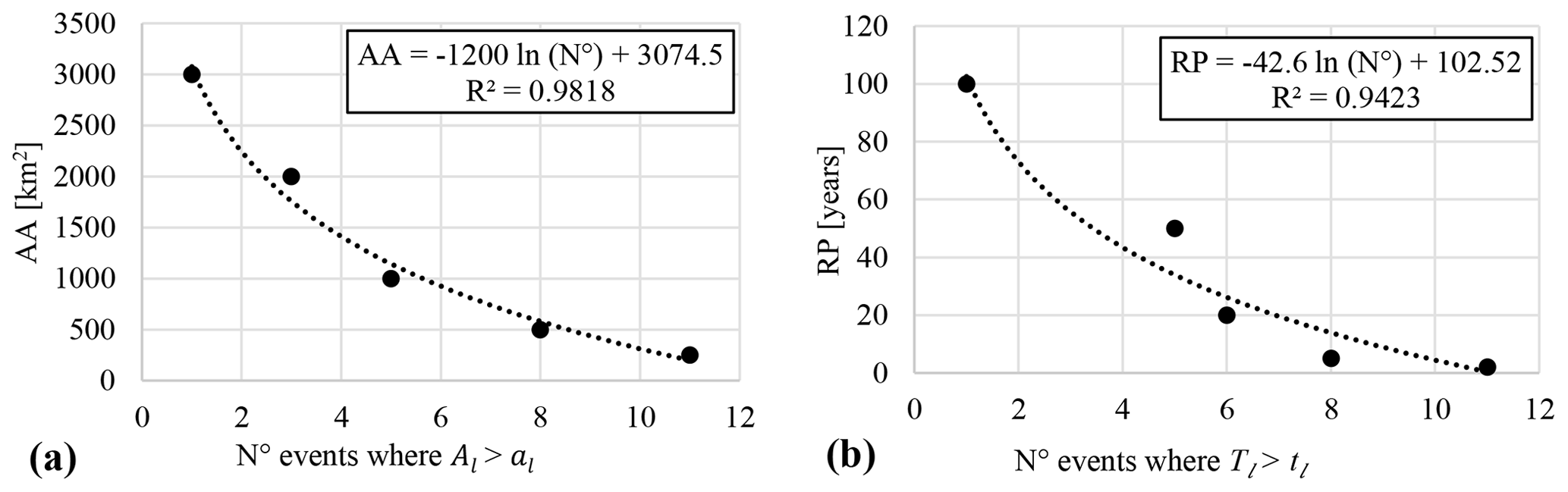
Figure 7 Frequency–magnitude relationship for (a) affected area (AA) parameter and (b) return period (RP) parameter. N^o is the number of events analysed in the study.

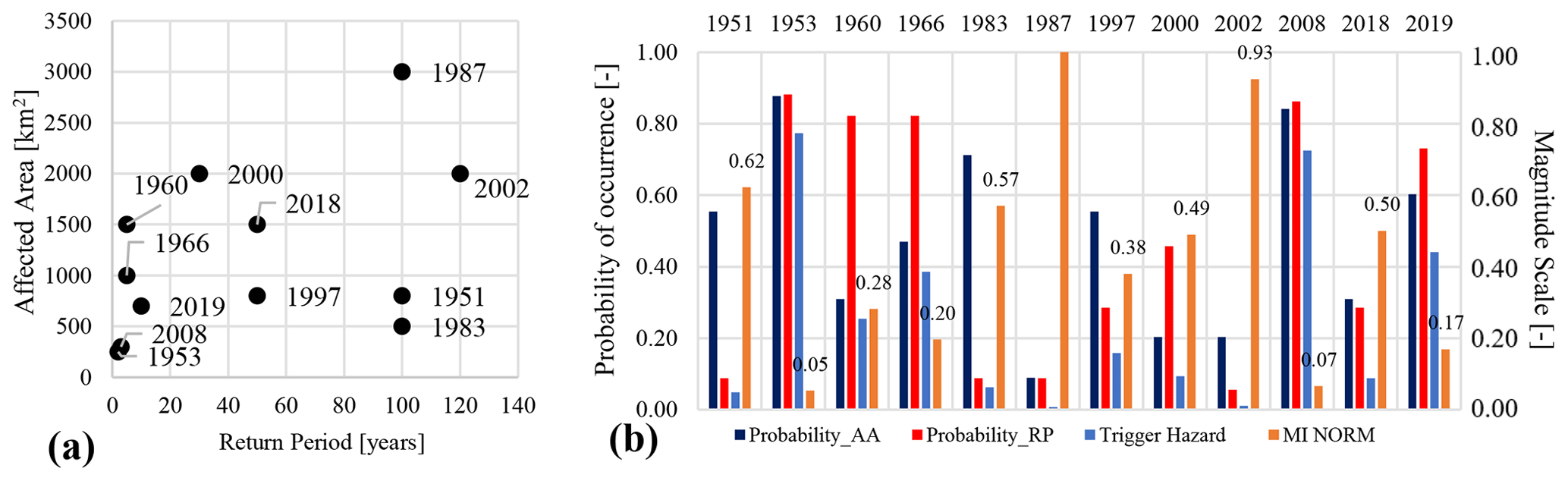
Figure 8 (a) Correlation between RP and AA parameters and (b) determination of the probability of occurrence of AA, the RP, and the trigger hazard for dataset events.

According to Corominas et al. (2014) and Guzzetti et al. (2005) and following the methodology proposed in Eqs. (2) and (3), we have moved further in considering both the RP and AA for determining the trigger hazard and magnitude. First of all, the FMCs have been established, allowing us to define the probability of spatial and time occurrence as a function of the parameters AA in Fig. 7a and RP in Fig. 7b. Secondly, AA has been plotted against the RP in Fig. 8a, and their low statistical correlation was observed. Then, considering Eq. (3a), the trigger hazard has been defined and reported in Fig. 8b. We can see that the trigger hazard is higher when the probabilities of spatial and temporal occurrence are higher. In particular, 1953, 2018, and 2019 represent the most hazardous events with lower RPs and AA. On the other hand, 1987 and 2002 represent the least hazardous events because, from a probabilistic viewpoint, they exhibit both the highest return period and the largest extent. Applying Eq. (3c) the trigger hazard has been translated into the magnitude index (MI), normalized in respect of its maximum and shown in Fig. 8b. We can see that the MI has highlighted 1987 and 2002 as the most severe events. On the other hand, 1953 and 2008 are depicted with the lowest magnitudes. An intermediate magnitude ranking was assessed for the 1951, 1983, 1997, 2000, and 2018 events, confirming historical evidence.

4.3 Approach 2 – EC intensity analysis and SLPT index

In the second approach, we applied the NCM described in Eq. (4). Using the NCEP data, atmospheric pressure gradients, wind velocities, and air masses advection through the Alpine region, the model components in Eqs. (5b)–(7b) and (8c) were studied.

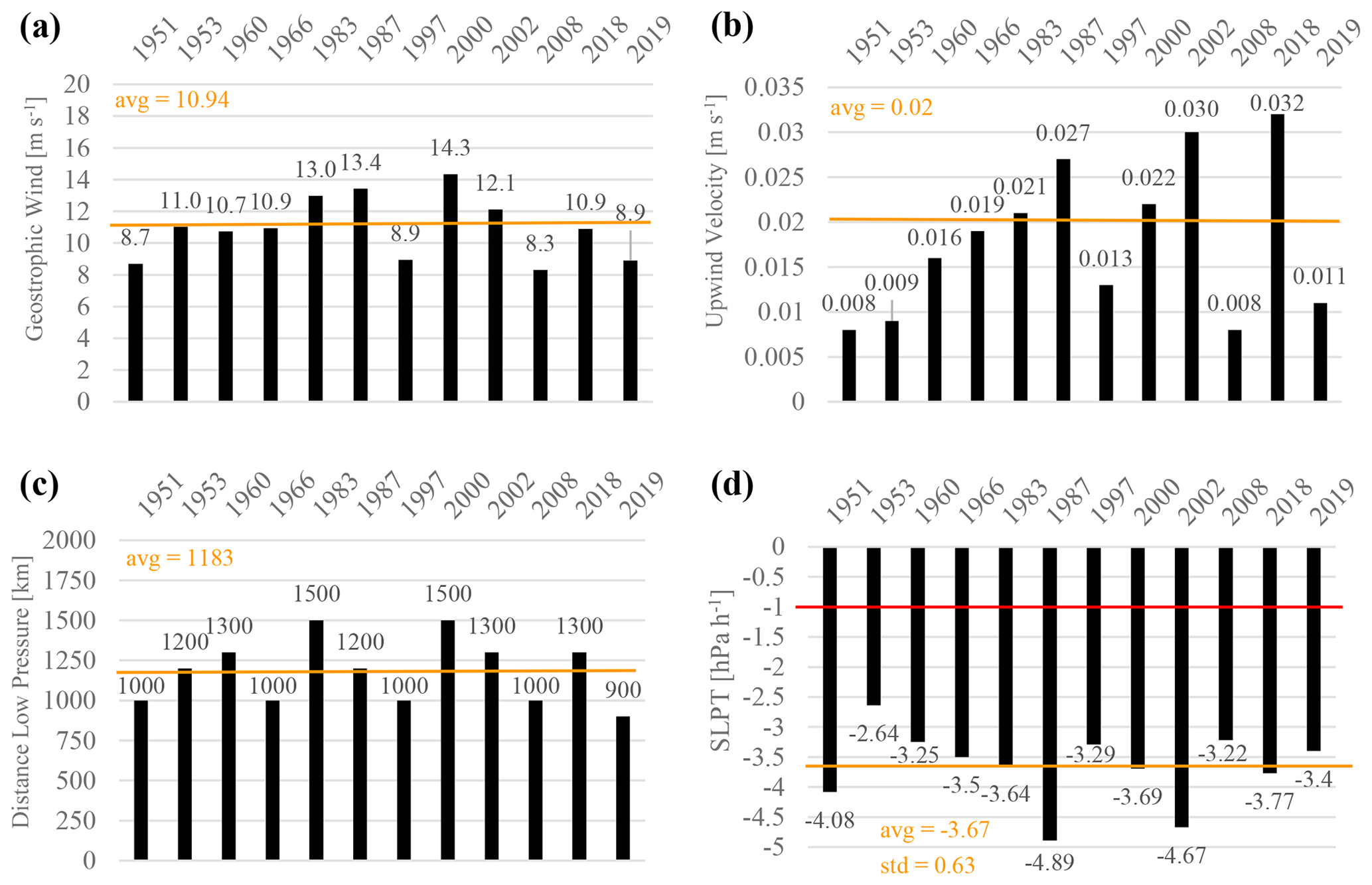
Figure 9 (a) Upwind velocity and (b) geostrophic wind velocity calculated for the T₁ term and (c) Δs₂ considered for the T₂ and T₃ terms. (d) The sea level pressure tendency (SLPT) index for the event analysed is computed. Orange lines represent the averages across the dataset while the red line indicates the threshold of explosive cyclogenesis (1 hPa h⁻¹).

For determining the T₁ term (Eq. 5b, upper-layer divergence), the geostrophic wind velocities were estimated. Geostrophic wind is the theoretical wind that would result from an exact balance between the Coriolis force and the pressure gradient force. It represents a first approximation of the general circulation of the air masses at a regional scale. Intense geostrophic velocities are generally associated with strong EC structures (Andrews, 2010; Martin, 2006; Stull, 2017). As reported in Fig. 9a, geostrophic velocities were higher for 1983, 1987, 2000, and 2002, a sub-group of the most intense events of our dataset. Upwind velocities in Fig. 9b are also correlated with the presence of sustained geostrophic winds. Again 1987, 2002, and now 2018 have shown the highest values of the entire dataset.

For determining the T₂ and T₃ terms (Eq. 6b, boundary layer pumping, and Eq. 7b, advection), the air masses' evolutionary paths were examined. Figure 9c shows the short distance Δs₂ between the low pressure (L) and Sondrio Province. We can see that the relative position of ECs does not vary too much, 1183 km on average. This represents a characteristic of the EC structures that tends to evolve across the Mediterranean and the Alpine area similarly. Nevertheless, some seasonal changes can be appreciated by looking at the advection path followed by the low-pressure centre (L). The larger part of the autumnal events exhibits a meridian motion of the low pressure from the northern part of Europe (North Sea) to the southern part, entering the Mediterranean Sea and moving eastward following the Rossby wave track (Rotunno and Houze, 2007; Stull, 2017). This is the case for the 1960, 1966, 2000, 2002, and 2018 events that occurred between September and November. Summer events of 1951, 1953, 1987, 1997, and 2019 exhibit a low-pressure tracking path that did not cross the Alps mountain range. This fact can be explained by considering that Rossby waves are in general shifted northward during the summer period (Grazzini and Vitart, 2015; Martin, 2006). This is reflected in the events that affect the southern side of the alpine region which are more rapid, less persistent, and locally intense but not well organized, such as the typical autumnal EC.

The T₄ term (Eq. 8c) is represented by a linear function of the daily rainfall rates (RRs) considered in the precipitation analysis. In the formulation adopted we made strong assumptions to make the problem more tractable. This is the only component that depends on the accurate estimation of the ground-based rainfall data.

After calculating the intermediate components T₁, T₂, T₃, and T₄, the sea level pressure tendency (SLPT) index of Eq. (4) was determined (Fig. 9d). Firstly, we can see that all these ECs have been characterized by explosive cyclogenesis. This definition applies when an extratropical cyclone exhibits a low-pressure deepening of 24 hPa in 24 h, which corresponds to an average rate of 1 hPa h⁻¹ (Sanders and Gyakum, 1980). Looking at Fig. 9d, the SLPT index shows a range between −2.64 hPa h⁻¹, recorded for the 1953 event, and −4.89 hPa h⁻¹, recorded for 1987. The latter and 2002 (−4.67 hPa⁻¹) are reported to have been the EC structures with the highest intensity that affected the northern Lombardy area. An average value of the SLPT index is reported at around $-\mathrm{3.67}\pm \mathrm{0.63}$ kPa h⁻¹ which is compatible with the EC structures shown by NCEP maps.

Figure 10 Comparison between the MI and SLPT index, normalized. The events recorded in 1951, 1987, 2002, and 2018 have the highest magnitude, while the 1953 and 2008 events have the lowest values.

4.4 Comparison between the MI and SLPT index

The two methodologies proposed for the trigger magnitude assessment are now compared. The two indexes MI and SLPT have been normalized in respect of their maximum and are shown in Fig. 10a. We can observe that it is rather clear how the two indexes give a similar magnitude rank for the events examined in our dataset. Looking at bias errors, the mean absolute error (MAE) is computed at around 7 % and the root mean square error (RMSE) is about 10.3 %. The highest absolute error values were addressed by the 2008 and 2019 events. Moreover, we can show that two indexes are in accordance, identifying 1987 as the episode with the highest magnitude, followed by 2002 and 1951. The lowest-ranking scores are established for the 1953 and 2008 events which were already identified by I–D analysis as borderline for the Cancelli Nova and Ceriani thresholds. In the middle, we found 1960, 1966, 1983, 1997, 2000, 2018, and 2019, which were also depicted by historical chronicles as rather intense but not catastrophic for Sondrio Province. In Fig. 10b the MI and the SLPT index have been plotted against each other. From Fig. 10b it can be appreciated that the points lie on the diagonal and the correlation index R² is about 0.88, which is rather high and near to 1.

5 Discussion

Considering the results obtained, we discuss here the questions that our study aimed to address. The first was, “are the I–D thresholds and the RP evaluation enough for a complete description of meteorological triggering factors?” The I–D thresholds are typically used for geo-hydrological risk assessment, but some uncertainties about their reliability have arisen around two aspects: the choice of the best-fitted threshold and the threshold's dependency on the RP parameter.

Regarding the first aspect, the thresholds can distinguish critical or non-critical events, giving only a binary outcome of the event classification. Shifting up and down the curve or changing the curve, the same event can be detected as a false negative or a false positive respectively, and this fact may lead to a prediction error. In the specific case of our dataset, the Guzzetti, Peruccacci, and Crosta Frattini curves seem to overpredict these events, while the Caine curve was found to underpredict them. On the other hand, the Cancelli Nova and Ceriani curves have been demonstrated to be more suitable for interpreting our dataset. In this regard, the local thresholds seem to be more accurate than the regional ones, but uncertainties remain about their correct application and interpretation. In fact, some recent studies have suggested that further investigation around their parameters' definitions is required to improve detection performances. According to several authors (Bogaard and Greco, 2018; Kim et al., 2021; Lazzari et al., 2018) the threshold may exhibit dynamic behaviour, shifting up and down when considering the soil moisture and the antecedent cumulated rainfall especially for short-duration events. This important condition has normally been neglected in the past definition of the thresholds, treating all the triggering events as uniform from a statistical point of view. Therefore, a wise disaggregation of these events in terms of antecedent conditions should be applied for creating a new threshold set that highlights the sensibility to those variables. In our opinion, this may help to improve further the performance of the I–D methodology especially for locally based thresholds under the reasonable assumption of a uniform spatial susceptibility of the territory. On the other hand, for the regional events, we think that the improvements would be less effective because other factors related to the more heterogeneous area, such as morphological or geological predisposing causes, may also play a more important role (Peruccacci et al., 2017). Including the RP in the threshold analysis can be useful to determine a preliminary magnitude ranking. Even though higher RPs are generally founded at a higher distance from the curve, the relative distance between the I–D point and the reference threshold cannot be always considered a proxy for the event magnitude. According to Gao et al. (2018) this assumption has not been so thoroughly reported, and this was also confirmed in our reanalysis study. A possible explanation can be found in the way the RPs are estimated. In principle, this interpretation of the trigger's magnitude is still valid only at a very local scale but cannot be adopted in our study since the GEV parameters used in RPs have changed in each rainfall episode. Our results have highlighted this fact two times, showing different point–threshold distances with respect to the same RP values. From this perspective, climate change will pose some challenges for updating the GEV in the future, considering that no stationary processes could affect the statistical distribution of critical precipitation (Albano et al., 2017b; Gariano and Guzzetti, 2016). This may add further uncertainties to this interpretation that considers only I–D thresholds and RPs for event magnitude estimation.

These two important observations represent a critical point in the I–D threshold methodology that has driven us to ask the following: “is the RP a good predictor of the magnitude?” Typically, the magnitude of a rainfall episode is described by the RP value, but this information is evaluated only from a time perspective. Taking inspiration from the landslide hazard definition proposed by Guzzetti et al. (2005), we defined a new magnitude index, MI, that was also representative of the “trigger energy”. In the definition of the MI, we have included the information about the trigger's spatial distribution AA. This choice aimed to address the lack of precise data about the landslide volumes, extents, or numbers, which are quantities considered for assessing an event magnitude scale (Malamud et al., 2004). The AA parameter can be interpreted as another proxy for the trigger's magnitude because indirectly it can describe the nature of the rainfall phenomena, distinguishing between a heavy, localized thunderstorm and persistent, more diffuse rain. As shown by our results, the RP and AA were uncorrelated, so both were considered for the assessment of the magnitude index (MI). The MI was estimated in our study with post-event information, but theoretically the index can be evaluated using weather forecasting, looking at expected rainfall rates and amounts across different areas. In this regard, local area meteorological models (LAMs) can be used to estimate the MI some hours in advance of the event. In our opinion, this represents one of the main advantages of using the MI because, in respect of the other magnitude indexes that require precise information about the “post-failure” effects (number of triggered landslides or peak discharge), the MI can be established using again only meteorological information, much like the SLPT index that we further propose.

As a matter of fact, we have implicitly answered the third question proposed: “can rainfall analysis be improved also considering other meteorological variables that are related to the trigger's magnitude?” The assessment of the MI has highlighted that the very local information about precipitation is not exhaustive, and spatial distribution of the rainfall is also needed to better comprehend the differences among the events. Moreover, if we are interested in the accurate trigger's description, looking only at the “final product” of a more complex meteorological process may not be enough (Copernicus C3S,2020; Rotunno and Houze, 2007; Stull, 2017). This is particularly true in mountain areas where the territory enhances the heterogeneity of the rainfall field (Abbate et al., 2021). For these reasons, other meteorological variables should be taken into account and included in the analysis. In our study, to pursue this goal we moved from a local perspective to a more regional one. This is crucial because it permits us to better describe the different precipitation types that may influence the occurrence of geo-hydrological failures (Corominas et al., 2014; Guzzetti et al., 2007). As an example, an intense thunderstorm during summertime could trigger a few shallow landslides or debris over a limited area (Abbate et al., 2021; Montrasio, 2000) in contrast to a persistent orographic rainfall that could affect an entire region, trigger diffuse terrain instabilities, and also reactivate deep-seated landslides (Longoni et al., 2011; Rotunno and Houze, 2007; Tropeano, 1997). In this regard, the local rain gauges series have been integrated with the NCEP reanalysis map data and the SLPT index was evaluated applying the theory of the Norwegian cyclone model. The implementation of this methodology has represented an innovative way to gain a comprehensive meteorological description of the rainfall triggers. In fact, in the NCM, the ground-based rainfall series represent only one term (T₄) that is involved in the EC intensification. The latter also depends on other processes: the upper-layer divergence (T₁), boundary layer pumping (T₂), and low-pressure advection (T₃). This additional information has been addressed to play an important role in EC evolution and helped us on better differentiate critical event characteristics.

The SLPT index formulation requires several data about triggers. These can be retrieved easily by looking at a reanalysis database such as the NCEP reanalysis maps. However, NCEP map interpretation is rather useful only for past events. Nowadays LAMs are much more suitable for interpreting the mechanism of ECs through a complex orographical area like the Alps (Ralph et al., 2004; Rotunno and Houze, 2007). In this regard, the NCM is still valid but the processes involved can be interpreted at a more detailed level with LAMs, avoiding some of the assumptions required by the NCM. The evaluation of the SLPT index should be intended as propaedeutic to further analysis, and it cannot be adopted in every situation. As we have foreseen from results, concerning the I–D thresholds methodology, the SLPT estimation requires moving from a very local perspective to a regional scale. This operation makes sense if the investigated area is extended to exclude very site-specific chain effects that can be triggered by isolated rainfall episodes, such as thunderstorm cells. Another important limitation on the applicability of the SLPT index regards the presence of a recognizable EC structure from meteorological maps. In fact, for weak ECs, the estimation of the trigger's magnitude may bring larger errors. In our study, this fact was experienced for the cases of 1953, 2008, and 2019 and was confirmed through visual inspection of NCEP maps. In these situations, the rainfall analysis should be restricted to a more local domain, trying to also include LAM outputs and radiosonde and satellite data (Abbate et al., 2021), and the application of the MI could be much more appropriate for the magnitude estimation.

As a result of our study, we have compared the two indexes, the MI and SLPT index, to assess the magnitude of critical events. Even though they come from different theories, the MI is based on frequency–magnitude theory and SLPT has a physical meaning in the meteorology field, it is clear that they are in accordance in depicting the same critical events with the highest magnitudes. This outcome has found confirmation in the qualitative information we retrieved in the historical database. These results have demonstrated that a strong cause–effect relationship exists between the strength of ECs developed at a regional scale and the effects recorded on a local scale, especially for strong events. For the dataset examined, the SLPT comparison with the MI was rather encouraging, R²=0.88, and the additional information retrieved from NECP maps has sharply improved the rainfall reanalysis completeness. In our opinion, both proposed indexes are useful instruments for describing the magnitude of the rainfall-induced events, overcoming the uncertainties in the I–D threshold methodology.

6 Conclusions

This study presents an extended reanalysis of the meteorological triggering factors that have caused several geo-hydrological issues in the past in the alpine mountain territory of Sondrio Province, northern Lombardy, Italy. Excluding the predisposing geomorphological causes in the area, attention was given to the characteristics of the rainfall. The main goal of our study was to assign a quantitative magnitude ranking to the meteorological trigger, following two approaches.

In the first one, the I–D threshold curve analysis was considered to identify critical rainfall events. We have demonstrated that the events fit some I–D thresholds, in particular the local thresholds of Cancelli Nova and Ceriani, and that the distance from the curve does not necessarily mean that an event has a higher RP. For this reason, to assign a magnitude to each of the events, we proposed the MI, which integrates the return period and the spatial extent of the event. The MI was determined analytically starting from the frequency–magnitude theory, according to the assumption that the event's magnitude was also a function of the spatial distribution of the trigger, described by the parameter AA. In the second approach, the trigger's analysis was conducted from a simply meteorological viewpoint, evaluating the strength of the extratropical cyclone structure through the NCM. Using the information of NCEP reanalysis maps, the SLPT index was determined and interpreted as another trigger magnitude index, much like the MI.

The two indexes have been compared, showing good agreement in the assessment of a magnitude ranking for the studied events. The SLPT index has confirmed the important relationship between the EC's intensity at a regional scale and the corresponding trigger's magnitude recorded locally, described by the MI. The two indexes are based on meteorological data; therefore, they may have an application in the nowcasting meteorology field. This could represent an important advancement, especially for the early warning systems adopted by municipalities for geo-hydrological risk mitigation.

In view of the future climate change that, with high confidence (Faggian, 2015), will affect the Mediterranean and the Alpine environment, extreme meteorological events are supposed to increase (Ciervo et al., 2017; Gariano and Guzzetti, 2016; Moreiras et al., 2018) and geo-hydrological hazards may also rise in frequency. Our study moves in this direction, trying to extend the interpretation of rainfall triggering factors through a more meteorological perspective.