the Creative Commons Attribution 4.0 License.
the Creative Commons Attribution 4.0 License.
 | 03 Jun 2021
Uncertainty analysis of a rainfall threshold estimate for stony debris flow based on the backward dynamical approach
Marta Martinengo
Daniel Zugliani
A rainfall threshold is a function of some rainfall quantities that provides the conditions beyond which the probability of debris-flow occurrence is considered significant. Many uncertainties may affect the thresholds calibration and, consequently, its robustness. This study aims to assess the uncertainty in the estimate of a rainfall threshold for stony debris flow based on the backward dynamical approach, an innovative method to compute the rainfall duration and averaged intensity strictly related to a measured debris flow. The uncertainty analysis is computed by performing two Monte Carlo cascade simulations: (i) to assess the variability in the event characteristics estimate due to the uncertainty in the backward dynamical approach parameters and data and (ii) to quantify the impact of this variability on the threshold calibration. The application of this procedure to a case study highlights that the variability in the event characteristics can be both low and high. Instead, the threshold coefficients have a low dispersion showing good robustness of the threshold estimate. Moreover, the results suggest that some event features are correlated with the variability of the rainfall event duration and intensity. The proposed method is suitable to analyse the uncertainty of other threshold calibration approaches.
- Article
(4953 KB) - Full-text XML
- BibTeX
- EndNote


In mountain regions, rainfall-induced natural phenomena, as shallow landslides and debris flows, are relatively frequent events that have a significant impact on the territory in which they occur, causing damages and, in some cases, casualties (Fuchs et al., 2013; Dowling and Santi, 2014; Cánovas et al., 2016). The risk management of these phenomena is crucial to reduce their effects on the territory, and it is based on both active and passive mitigation strategies. An early warning system is an example of a passive mitigation tool (Huebl and Fiebiger, 2005) as it allows the activation of prevention measures (e.g. evacuation sets out in the civil protection plans) before the expected event occurs.
The early warning systems for these phenomena are mainly based on rainfall thresholds (Chien-Yuan et al., 2005; Segoni et al., 2018), namely rainfall conditions beyond which the occurrence probability of a rainfall-induced event is considered significant. In this framework, most rainfall thresholds are power-law relations expressing the rainfall event cumulated or intensity as a function of the event duration (Segoni et al., 2018). A considerable literature deals with this topic (e.g. Caine, 1980; Guzzetti et al., 2008; Winter et al., 2010; Jakob et al., 2012; Staley et al., 2013; Marra et al., 2014, 2016; Zhou and Tang, 2014; Iadanza et al., 2016; Pan et al., 2018).
In some studies rainfall thresholds concern a wide typology of phenomena (Segoni et al., 2018), other works focus on both shallow landslides and debris flows (e.g. Baum and Godt, 2010; Cepeda et al., 2010), other works focus only on shallow landslides (e.g. Giannecchini, 2005; Frattini et al., 2009), and, finally, some studies are specifically conceived for debris flow (e.g. Nikolopoulos et al., 2014; Giannecchini et al., 2016; Li et al., 2016).
Power-law thresholds can be derived in the following way. Given a historical dataset of rainfall-induced events, the rainfall associated with each event is determined and described in terms of the couple of synthetic quantities employed in the threshold (e.g. rainfall event cumulated–event duration). Classically, these quantities are defined only on the basis of a hyetograph analysis (Segoni et al., 2018), without considering the characteristics of the rainfall-induced phenomenon. In a log–log plane, the resulting set of couples becomes a cloud of points and the power-law function is a straight line. Starting from these couples set, the threshold is determined by locating the straight line in the log–log plane using one of the several estimate strategies available in the literature, e.g. manual methods, statistical approaches and probabilistic procedures (Guzzetti et al., 2007; Segoni et al., 2018). The result is the calibrated rainfall threshold.
One of the critical issues of the calibration is the uncertainty related to both data and model parameters (Gariano et al., 2020). Here with the term “model” we indicate generically a single equation or a set of operations that, given some input data and model parameters, provide an output. In the case of the rainfall threshold, the uncertainties derive mainly from direct data error measurements (e.g. in rainfall), from the non-unique definition of the models parameters (e.g. distance within which to select the rain gauge to define the event precipitation) and from the strategy used to calibrate the threshold. The result is an uncertainty framework that can significantly impact the threshold estimate.
Some studies have already investigated the uncertainty in threshold determination, focusing on some aspects that can affect the hyetograph or the event synthetic quantities used in the threshold. For instance, Nikolopoulos et al. (2014) have analysed the consequences of the spatial variability of the precipitation while Marra (2019) and Gariano et al. (2020) have investigated the effects of the rainfall temporal resolution. Moreover, the uncertainty arising from the choice of the reference rain gauge and the differences between the radar and the rain gauge measurements have been examined in Rossi et al. (2017). Besides, the effect of the uncertainty in triggering rainfall estimate has been investigated in Peres et al. (2018), while Abraham et al. (2020) have analysed the consequences of the scale of analysis, the rain gauge selection and how the intensity is quantified.
Rosatti et al. (2019) have introduced an innovative method to calibrate an intensity-duration rainfall threshold for stony debris flow, a particular type of debris flow, frequent in some mountain areas as in the Alps, in which the presence of silt and/or clay in the mixture is negligible and the internal stresses are mainly caused by the collision among the particles (e.g. Takahashi, 2009; Stancanelli et al., 2015; Bernard et al., 2019). The new method, called the backward dynamical approach (BDA), starts from the knowledge of the volume of sediments deposited after an event, and, thanks to a schematic description of the stony debris-flow dynamic, it is able to identify, in the related hyetograph, the rainfall event volume, intensity and duration strictly pertaining to the debris-flow event. Hence, the BDA differs from the classical literature approaches since the synthetic quantities describing the rainfall events are defined involving not only the forcing (i.e. the hyetograph) but also the dynamic of the rainfall-induced event.
This work focuses on the uncertainty deriving from data and parameters inherent to the BDA, leaving out the uncertainty related to the hyetograph, already investigated in the literature. In particular, the aim is to perform an uncertainty analysis on the threshold calibration to check the robustness of the BDA. To reach this goal, among the different strategies and methods available in the literature (e.g. Helton et al., 2006; Coleman and Steele, 2018; Hofer, 2018), we have chosen the Monte Carlo (MC) approach. With this tool, we have developed a proper methodology composed of two MC cascade simulations, and we have applied it to a dataset concerning a specific study area. Detailed analysis of intermediate and final results have also been performed to better understand the uncertainty analysis outcomes.
The paper structure is the following. A brief description of the BDA method is presented in Sect. 2. The study area and data are described in Sect. 3. The method used to assess the uncertainty propagation in the BDA-based threshold calibration is described in Sect. 4. The obtained results are presented and discussed in Sect. 5. Conclusions end the paper.
As mentioned in the Introduction, the BDA determines the rainfall event intensity and duration, namely the couple (I,D), associated with a stony debris flow, by using not only the hyetograph but also information concerning the occurred debris flow.
The BDA starts from the knowledge of the deposited volume Vdep occupied by the sediments after a debris-flow event. Thanks to a simplified global volumetric description of the debris-flow dynamic (Fig. 1), the rainfall volume pertaining to the debris flow , defined as the volume of water necessary to convey downstream Vdep as a mixture, can be expressed as
where cb is the concentration of the sediment in the bed, constant and assumed equal to 0.65 (Takahashi, 2014), and c is a reference volumetric solid concentration of the given debris flow.
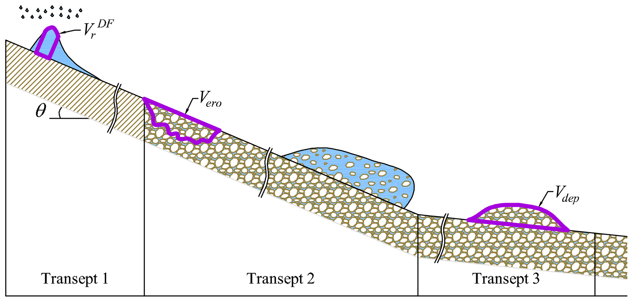
Figure 1Conceptual Lagrangian volumetric description of the debris-flow dynamic from Rosatti et al. (2019). The scheme is divided into three transepts: transept 1 is characterised by the run-off formation; the bed material erosion and the achievement of equilibrium conditions occur in transept 2; transept 3 is characterised by the deposition of sediments with water entrapment. is the rain volume pertaining to the debris flow, Vero is the bed volume variation related to the erosion, Vdep is the deposited volume occupied by the sediments and θ=arctan (if) is the inclination angle of the bed with respect to a reference horizontal direction.
The expression of Takahashi (1978) is valid in permanent and uniform conditions, and it can be used as reference concentration:
where if is the bed slope, ψ is the dynamic friction angle of the sediments and is the sediment relative submerged density, where ρl and ρs are, respectively, the liquid and solid constant density. Δ is constant and assumed equal to 1.65 (e.g. Prancevic and Lamb, 2015). According to the assumptions of the BDA, the reference concentration is evaluated considering the bed slope in the last portion of the debris-flow channel, just upstream of the deposition area. This means that the information concerning the triggering conditions and the detailed evolution of the debris flow in the upper part of the basin are not considered.
The rainfall volume pertaining to the debris flow can also be expressed as the product of the rainfall volume per unit area E and the event basin area Ab,
from which a backward dynamical expression for the rainfall volume per unit area can be obtained by equating Eq. (1) with Eq. (3):
On the other hand, E can be obtained from the forcing of the phenomenon, namely the hyetograph. Under the assumption of uniform rainfall over the basin, the hydrological expression for E is
where i(t) is the measured rainfall intensity, and t1 and t2 are the unknown start and end times related to the debris-flow duration. In the absence of detailed data of the event, these times are expressed as
where tmax is the instant of maximum intensity during the event, and Δt1 and Δt2 are unknown intervals. These intervals can be obtained by equating the right-hand side terms of Eqs. (5) and (4):
Because of the measurement technique, i(t) is a piecewise constant function on time intervals δt, namely i(k). Consequently, the reference times becomes t=kδt, , Δt1=n1δt and Δt2=n2δt, where M is the number of time intervals that identifies the peak, and now n1 and n2 are unknown integers. In addition, the integral in Eq. (7) must be rewritten in discrete form (namely a summation), and the previous equation cannot be satisfied exactly.
An approximation algorithm, able to determine in a univocal way the unknowns, can be introduced: starting from zero and increasing one unit alternatively n1 and n2, the first couple , for which the condition
is satisfied, is the searched couple. If a zero-intensity interval is reached, the sum stops being symmetrical with respect to M, and only either n1 or n2 is increased until the previous relation is satisfied.
Finally, the duration D and the average intensity I can be expressed as
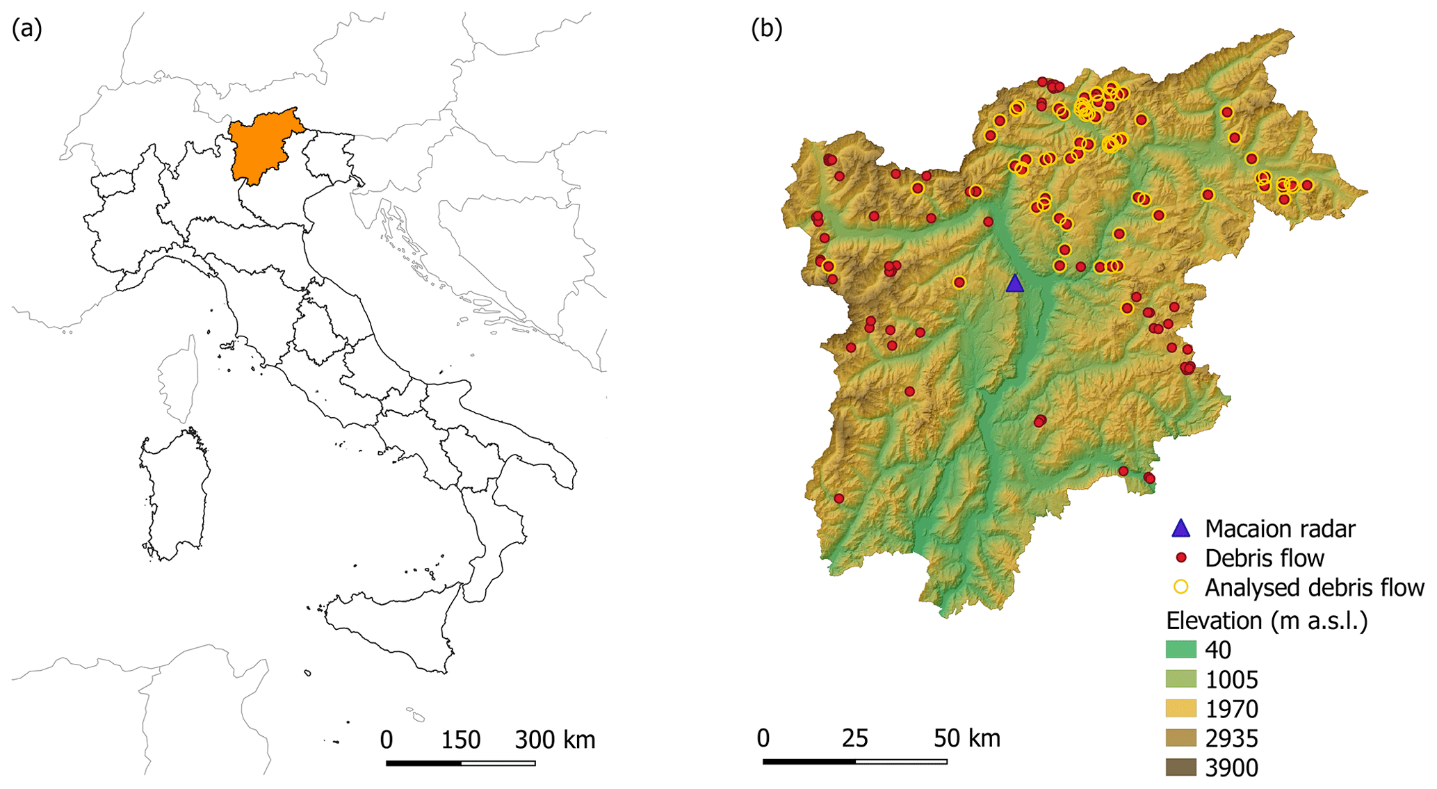
Figure 2(a) Location of the Trentino-Alto Adige/Südtirol region (Italy) and (b) the Macaion radar and debris-flow events: red dots show all debris flows, while yellow circles highlight the suitable ones for the study.
Once the (I,D) couple is computed for each event of the available dataset, the rainfall threshold is estimated by using the frequentist method (e.g. Brunetti et al., 2010; Peruccacci et al., 2012). According to this method, the (I,D) couples are plotted in a log–log I–D plane, and a straight line fitting these points is determined. The slope and the intercept of this straight line are the logarithms of the coefficient of the following power law:
The rainfall threshold is then obtained translating vertically the straight line in the log–log I–D plane so that the non-exceedance probability of the dataset events (namely the occurrence probability of debris flows related to (I,D) points located below the threshold) is equal to a given value. The final expression is
in which .
For more details on the BDA and the frequentist method, we refer the reader to the above-mentioned references.
The study area and data used in this analysis are the same as those used in Rosatti et al. (2019). In particular, the study area is the Trentino-Alto Adige/Südtirol region (also known as Trentino-South Tyrol), in the north-east of the Italian Alps (Fig. 2a). The region covers 13 607 km2, has an altitude range between 40 and 3900 m a.s.l. with mean about 1600 m a.s.l. (Fig. 2b), and has a climate characterised mostly by a continental regime (Bisci et al., 2004; Nikolopoulos et al., 2014).
The regional agencies between 2006 and 2016 have reported 161 debris flows (Fig. 2b), but only 139 events present the survey of the deposits, whose volumes range between 100 and 50 000 m3. In every event, sediments are characterised by the absence or, at least, the negligible presence of silt and clay thus resulting in stony debris flows.
The rainfall data related to these events derive from a radar located in a central position with respect to the region, on Mt Macaion at 1866 m a.s.l. (Fig. 2b). A C-band Doppler weather radar measures the reflectivity Z over an area of 120 km of radius, and the rainfall is computed converting Z into precipitation intensity I (e.g. Uijlenhoet, 2001). Since radar data in mountain regions are typically affected by the beam shielding (Germann et al., 2006), which can cause errors in the measurements, the debris-flow events located in an area with a weakening of the signal greater than 90 % have been excluded from the dataset. Overall, the debris flows suitable for the analysis were 84 and are highlighted in Fig. 2b with circles.
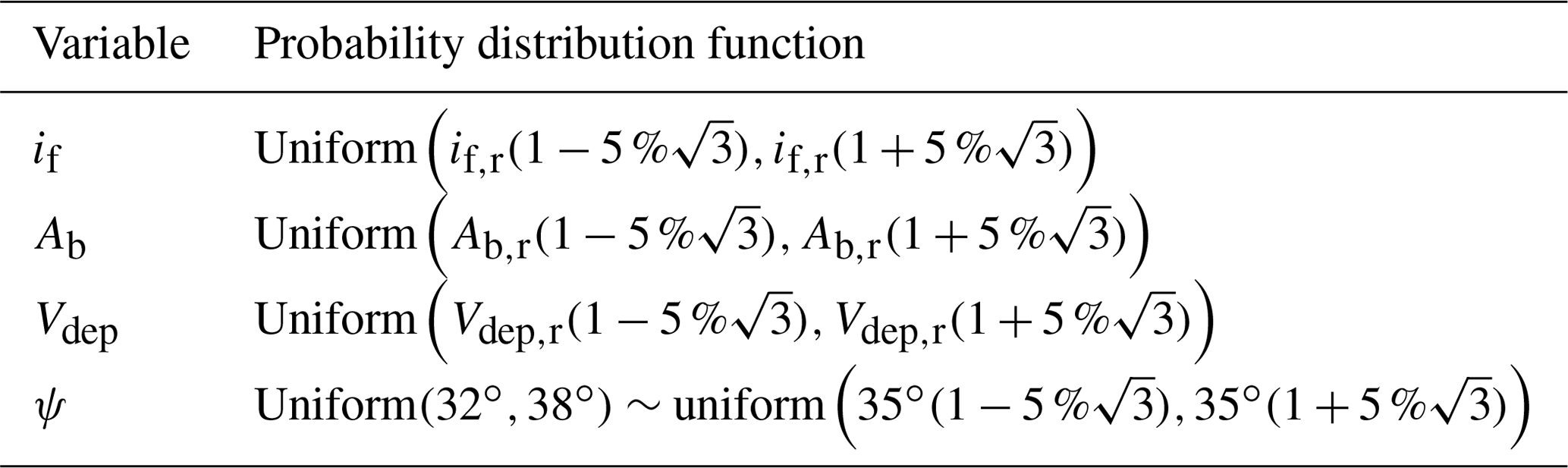
Table 1Probability distributions of the uncertain variables for each event. if,r, Ab,r and Vdep,r are the event reference values of the average slope, the basin area and the deposited sediments respectively.
Additional data required for the BDA, namely if, Ab, ψ and i(t), were defined for each event in the following way. The basin outlet was located downstream of a segment with a sufficiently constant slope just upstream of the deposition area, and the upstream basin area was determined. Then, if was calculated as the mean slope of the last 50 m of the torrent upstream of the outlet point. Besides, due to the scarcity of sediments information, ψ was assumed to be equal to 35∘ for all the events. The hyetograph i(t) was computed at each instant averaging over the respective basin area the radar intensities. In this way, both the spatial and temporal variability of the rainfall were taken into account.
Starting from these data and setting the non-exceedance probability equal to 5 %, Rosatti et al. (2019) obtained the following threshold:
From now on, the quantities involved in the calibration performed by Rosatti et al. (2019) will be considered as reference values, and they will be indicated with a subscript r.
As described in Sect. 2, the BDA-based threshold calibration starts from the definition of the following input parameters and data for each considered event: if, Ab, Vdep, ψ and i(t). Subsequently, based on these values, what we call the “event characteristics” are computed for each analysed debris flow: first c (Eq. 2) and E (Eq. 4) and then D (Eq. 9) and I (Eq. 10). Finally, the (I,D) couples of the events are used to calibrate the threshold, namely to quantify the threshold coefficients a and b of Eq. (12).
Coherently to the estimate procedure, the uncertainty analysis of the BDA-based threshold calibration is divided into three parts (Fig. 3). First, the uncertainty characterisation of the input parameters and data is determined (Fig. 3a). Then, for each debris flow, the uncertainty analysis of the event characteristics is performed with an MC simulation, starting from the above-defined uncertain quantities (Fig. 3b). Finally, a further MC simulation is carried out to perform the uncertainty analysis of the threshold, using as input the (I,D) couples of the events obtained from the first MC simulation (Fig. 3c). In this way, the impact of the uncertain parameters and data on the threshold is quantified. All the analyses are performed using the R software (R Core Team, 2013).
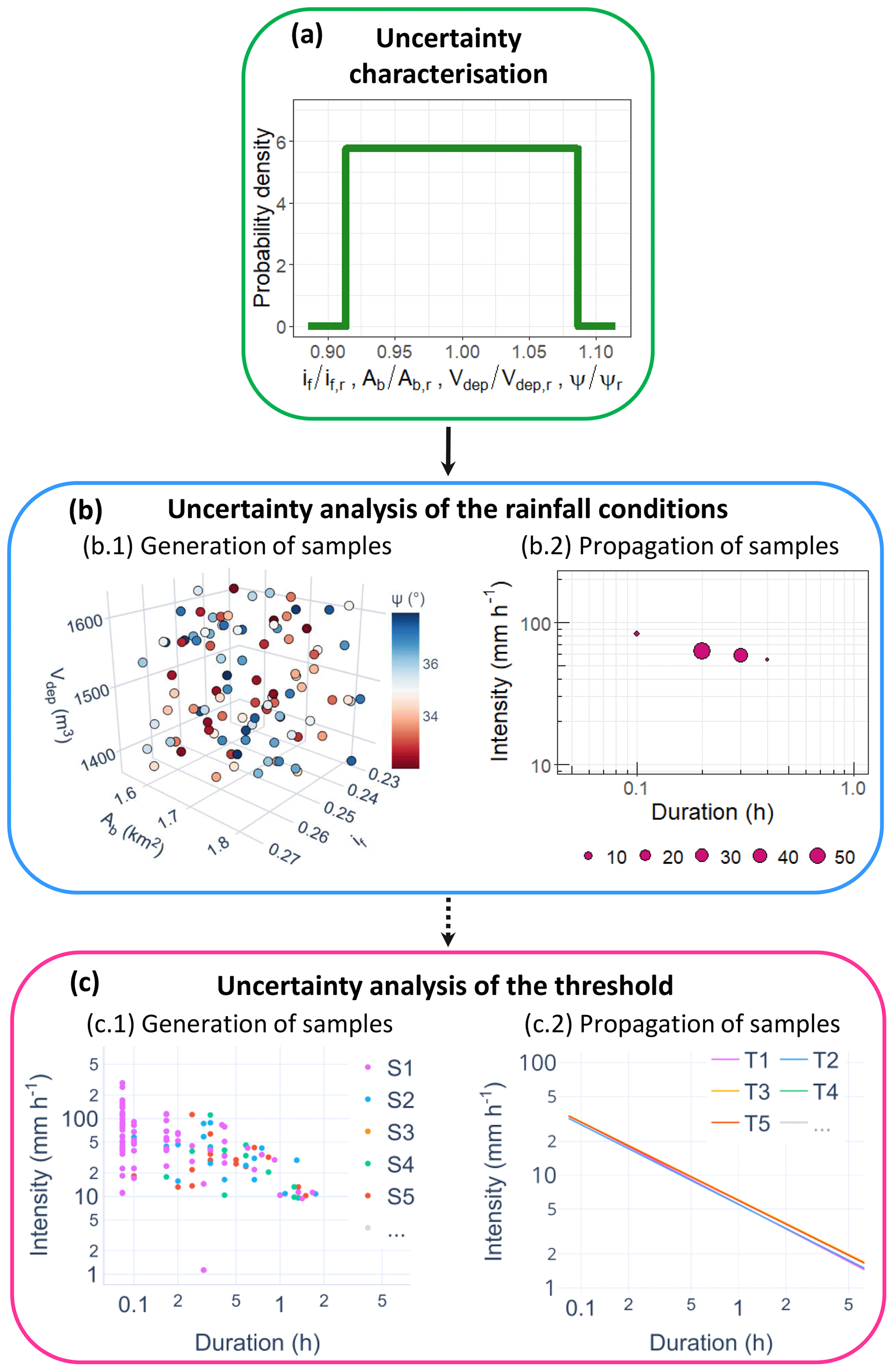
Figure 3Scheme of the uncertainty analysis performed with two cascade MC simulations. (a) Uncertainty characterisation of the parameters and data: the non-dimensional form of the uncertain parameters and data, obtained by dividing the variables by the reference values, are assumed to be uniformly distributed. (b) First MC simulation to compute the uncertainty analysis of the event characteristics for each debris flow: (b.1) sample generation performing the Latin hypercube sampling (LHS) and (b.2) propagation of samples to compute the event characteristics. The dot size in the log–log I–D plane indicates the absolute frequency of obtaining the (I,D) couples. (c) Second MC simulation to perform the uncertainty analysis of the threshold: (c.1) random sample S generation (one of the previous obtained (I,D) couples for each event) and (c.2) propagation of samples to estimate the thresholds T.
Regarding the uncertainty characterisation, as explained in the Introduction, the focus of this study is on the uncertainty in the physical and morphological parameters and data used in the BDA to describe, in a simplified way, the debris-flow dynamic. Therefore, in this analysis, the variables considered are if, Ab, Vdep and ψ. According to their estimate, described in Sect. 3, these variables are mainly affected by epistemic uncertainty due to measurement and estimate errors and lack of information (Oberkampf et al., 2004). The characterisation of the uncertainty in the variable, namely the probability distribution function (PDF) of their values, has to be defined both in term of distribution type and statistical quantities (e.g. mean and variation coefficient CV) (Fig. 3a). Lacking certain data concerning the PDFs, according to Marino et al. (2008), all the variables are assumed to be uniformly distributed, and, for each event, the means of the distributions are set equal to the corresponding reference values. Regarding the deviations from the means, ψ is the only variable whose variability is constrained by a validity range: for stony debris flow, according to Lane (1953) and Blijenberg (1995), ψ can vary between 32∘ and 38∘. Assuming 35∘ as the mean of the ψ distribution, the variability range (32∘, 38∘) can be obtained by imposing CV equal to about 5 %. The uncertainty in Vdep cannot be accurately estimated since the survey methodology, and the related measurement errors, used by regional agencies, is not univocal (Marchi et al., 2019). However, Brardinoni et al. (2012) has proposed, for a similar study area, a relative error of 10 % in the estimate of Vdep, namely a corresponding CV equal to about 5 %. Therefore, we assume that this uncertainty value is valid for this analysis. Moreover, the uncertainty in if and Ab is hardly quantifiable given their computation method. For these reasons and homogeneity, the degree of uncertainty of ψ and Vdep is considered suitable also for if and Ab. The resulting uncertainty characterisation is summarised in Table 1.
The procedure used to assess the propagation of the uncertainty in if, Ab, Vdep and ψ on the event characteristics (i.e. D, I, c and E), related to each debris flow, is schematised in Fig. 3b, and it is composed of two main steps. First, the input samples, namely the ordered sets of variable values in the form , must be obtained. These samples are generated by using the Latin hypercube sampling (LHS) (Fig. 3b.1), introduced by McKay et al. (2000). This method produces N samples starting with a division of each variable uncertainty range into N disjoint intervals of equal probability. Then, one value is randomly selected within every interval, thus obtaining N values for each variable. These values are then arranged in the LHS matrix, composed of N rows and k columns, where k is the number of the variables (four, in the specific case). In each column, the N values relevant to a single variable are inserted in random order (Helton et al., 2006). Each row of this matrix gives one of the N variable samples. According to Marino et al. (2008), to ensure accuracy, the sample size N should be at least greater than k. In this study, N is set to 100, and the (100×4) LHS matrix is generated for each event, based on the previously established PDFs.
Second, the event characteristics are obtained starting from each input sample, resulting in 100 (I,D) couples (Fig. 3b.2), together with the related c and E values, for each event. Therefore, the overall total of (I,D) couples obtained is , where 84 is the number of considered debris flows.
The uncertainty propagation in the threshold estimate is then quantified with a further MC procedure. In this case, a sample is generated selecting randomly one of the possible 100 (I,D) couples for each event, resulting from the previous MC simulation (Fig. 3c.1). Hence, one sample consists of 84 (I,D) couples. Following this procedure, 5000 samples are created and used to estimate as many thresholds (Fig. 3c.2), namely 5000 (a,b) couples.
5.1 Variability of the event characteristics
As described in Sect. 4, the outputs of the first MC simulation applied to the dataset are 100 possible event characteristics (i.e. D, I, c and E) for each debris flow. The relative variability of all these outputs is quantified through the computation of the CV of each event characteristics distribution. This allows providing a complete inspection and interpretation of all outputs. Then, the absolute variability is quantified through the computation of the variability range given by the difference between the minimum and the maximum values of the variable, and it is evaluated only for the D and I distributions. This analysis allows highlighting the variability of the (I,D) couples in the I–D plane for each event.
Table 2Coefficients of variation of the event characteristics related to each debris flow expressed as a percentage. CVD is the coefficient of variation of the duration distribution, CVI is the coefficient of the intensity distribution, and CVc is the coefficient of the concentration distribution and CVE is the coefficient of the rainfall volume per unit area distribution.
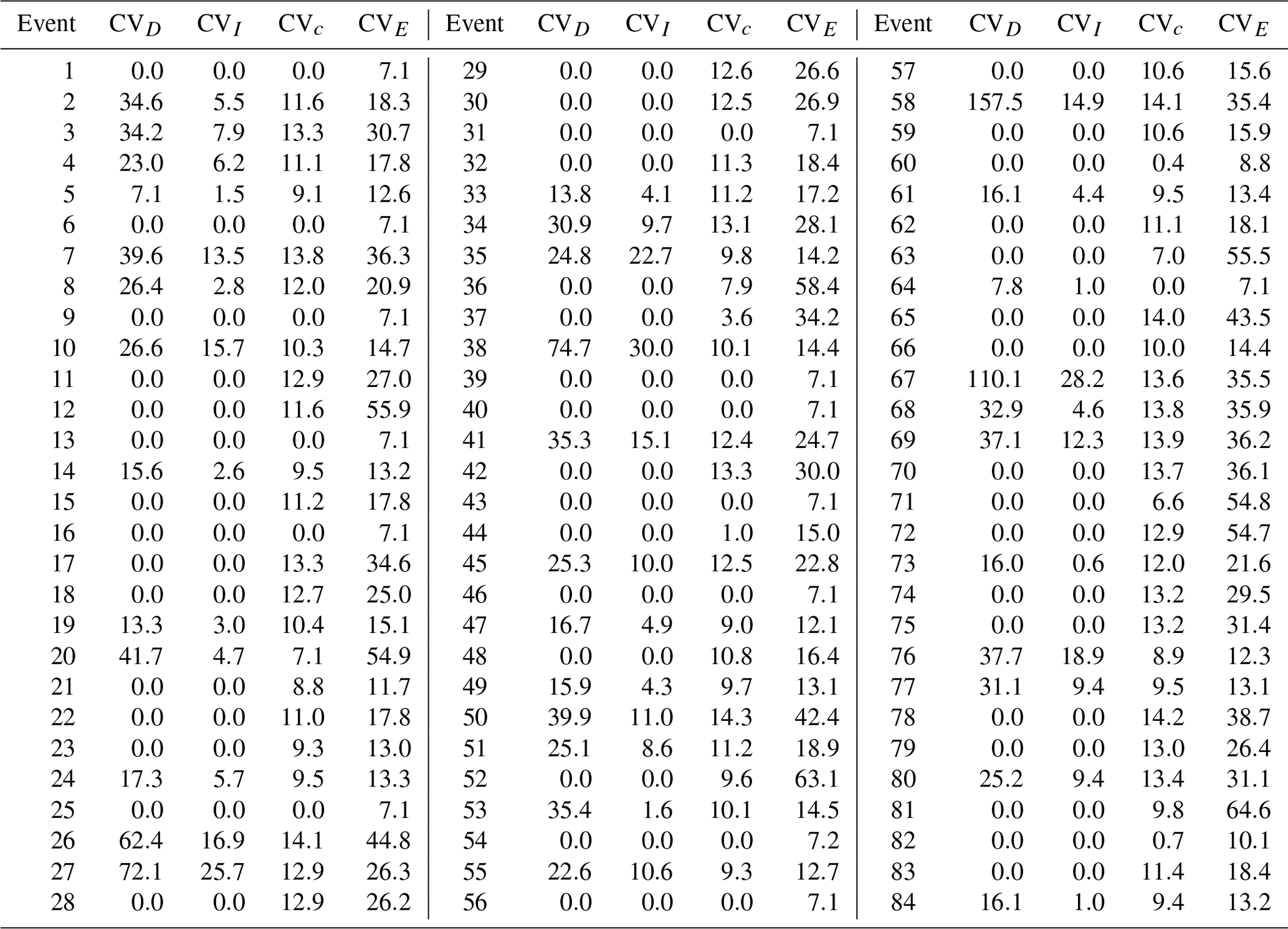
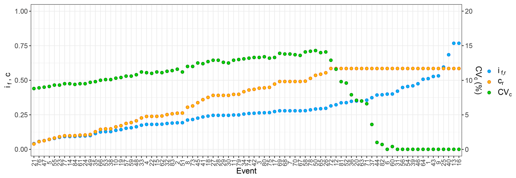
Figure 4Reference slope if,r and reference concentration cr and CVc of each event. The events have been sorted with increasing if,r.
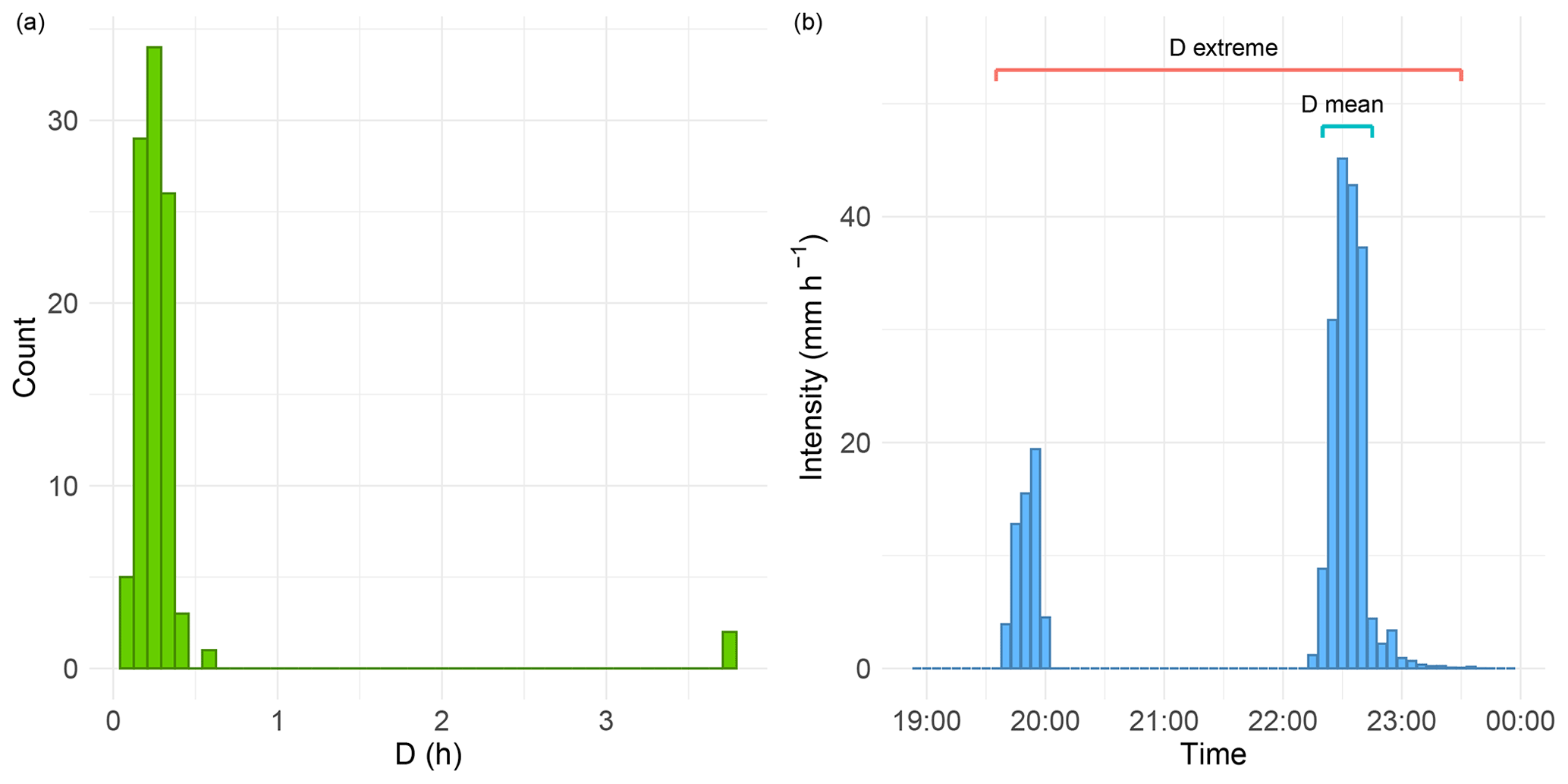
Figure 5(a) Duration distribution histogram and (b) hyetograph of event 58. The histogram shows the presence of an extreme isolated from the mass of the distribution. This extreme (D=3.75 h) is shown in the hyetograph and compared with the mean (D=0.32 h).
The CV, by definition, is a standardised measure of dispersion (Håkanson, 2000) and allows comparing the relative variability of the results independently of their measurement units (Abdi, 2010) and of their means. For this reason, the CV is chosen as the statistical quantity for comparing the relative variability between both the same characteristic of different events and different characteristics of the same event. The CVs of the distributions of D, I, E and c for each event are shown in Table 2. In the following, the trends and the differences in the CVs are highlighted and justified on the basis of some event aspects.
-
The D distributions have the largest and most variable CVs with respect to all the other event characteristics: CVD vary between 0 % and 157.5 %. The reason for this behaviour will be clarified later on.
-
The distributions of I are characterised by a lower spread with respect to the D distributions, with all the CVI values being within 0 % and 30.0 %. The reason for this behaviour is connected to the fact that I, by definition, is an average, and therefore the effects of the variable uncertainty are smoothed by the averaging. Also the reason why CVI can be zero will be explained later on.
-
In addition, the concentration distributions show a low spread. As c is characterised by an upper bound (i.e. 0.9cb), the CVc is strictly related to the proximity of cr to this maximum value and consequently, according to Eq. (2), to the value of if,r. As shown in Fig. 4, until the if,r is less than about 0.3, the CVc tends to go up by increasing the if,r since cr is sufficiently smaller than 0.9cb. Instead, if the if,r is between about 0.3 and 0.4, the CVc tends to decrease by increasing the if,r as c reaches the maximum, and it is equal to 0.9cb for an increasing number of if samples. Finally, the CVc becomes 0 % if the if,r is greater than about 0.4 as c is always equal to 0.9cb independently from the values of the if samples. However, even in the worst conditions in terms of variability, CVc is small and reaches a maximum value of 14.3 %.
-
The distributions of the volumes per unit area have CVE values that vary between 7.1 % and 64.6 %. It is worth noting that high uncertainty in the estimation of E does not necessarily imply large CVD and/or CVI (e.g. event 12) and vice versa (e.g. event 38). This suggests that the relative variability in I and D does not depend only on the relative variability in the needed rainfall volume per unit area but also on how the available rainfall volume is distributed into the hyetograph time intervals.
To better understand the variability of D and I, we classify the events into three categories based on the CVD values:
-
events with zero variability: CVD=0 %;
-
events with low variability: ;
-
events with high variability: CVD>30 %.
The first category comprises 48 events for which the 100 MC simulations have provided always the same (I,D) couple. For these events, the propagation of the variable uncertainty does not affect the (I,D) couple estimation resulting in . This type of result is related to two conditions:
-
Regardless of the uncertainty of the variable, the concentration is always equal to 0.9cb. In this case, also CVc is equal to zero (e.g. events 1, 13 and 25) and the variation in E is only due to the propagation of Ab and Vdep uncertainty (Eq. 4), namely CVE≃7.1 %. For these 14 events, such a small variation in E results in the constant computation of the same (I,D) couple.
-
Despite the fact that CVc is not zero and the CVE is greater than 7.1 % (e.g. event 28), the condition of Eq. (8) is satisfied, in all the 100 simulations, considering always the same hyetograph time intervals. A total of 34 events fall into this condition.
For the 19 events that belong to the second category, the uncertainty in the variables results in the computation of more (I,D) couples that, however, are relatively close to the mean values: the I and D distributions are characterised by a standard deviation much smaller than the mean.
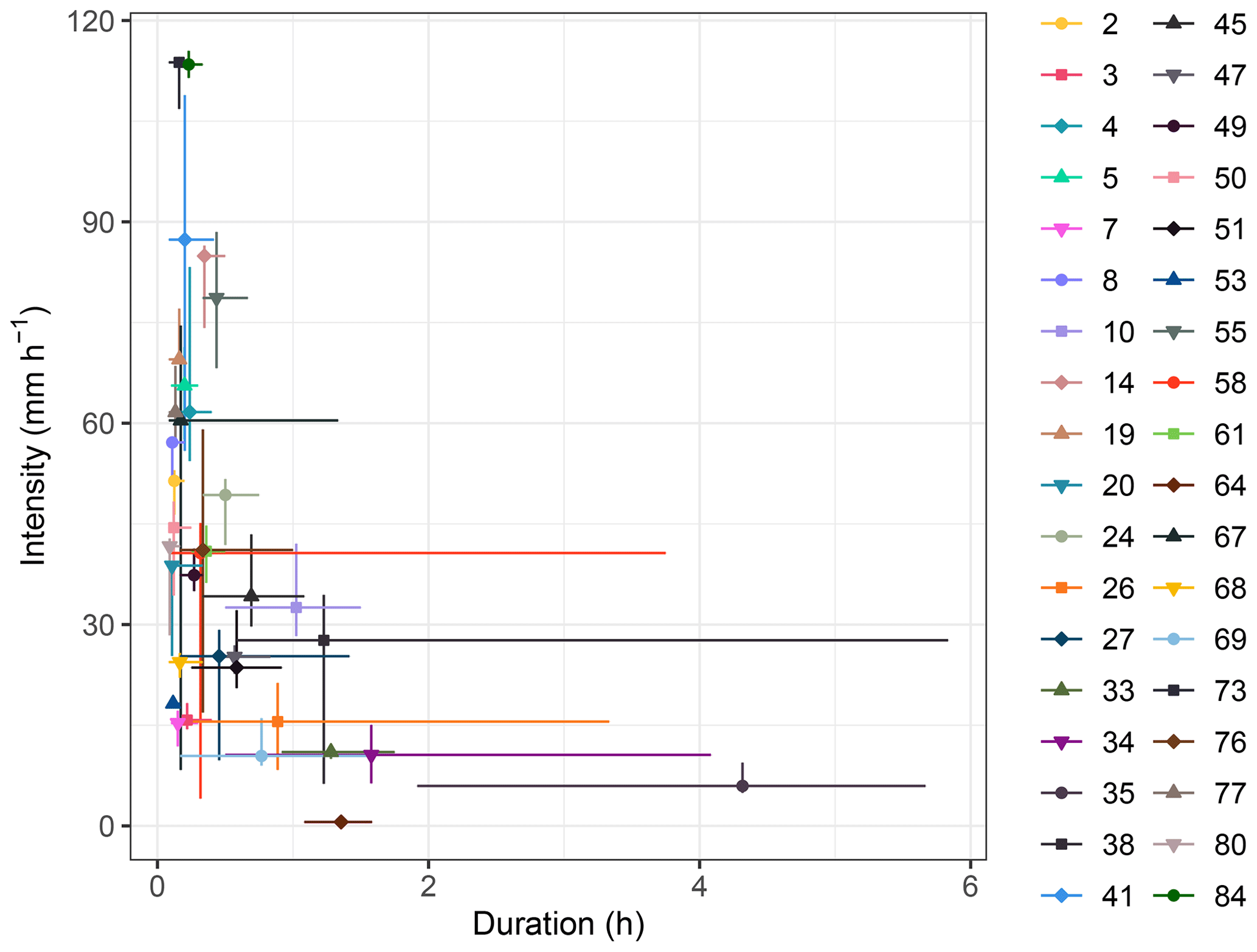
Figure 6Absolute variability in the (I,D) couples. The symbols are the mean values, and the horizontal and vertical lines are respectively the duration and intensity variability ranges. To make the graph clearer, the events with ranges equal to zero have not been represented and the linear scale is used for both axes.
The third category includes 17 events for which the uncertainty in the variables implies high values of CVD. This means that, for these events, the number of time intervals needed to satisfy the condition of Eq. (8) varies greatly with respect to the mean one: the variable uncertainty has a relatively great impact on the computation of D. Moreover, the highest values of CVD highlight the presence of extremes in the D distribution, namely of values of D very distant from the mean. Indeed, CV is very sensitive to the extremes (e.g. Chau et al., 2005; Arachchige et al., 2020), mainly if they are located in the right-hand tail of the distribution (Bendel et al., 1989). For instance, the effect of the extremes on the CVD is evident in event 58: the D distribution of this event has an extreme much greater than the mean (Fig. 5a). This is due to the presence of zero-intensity temporal instants in the middle of the hyetograph that must be considered (for two out of a hundred samples) to reach the highest values of E (Fig. 5b). This results in a high value of the standard deviation with respect to the mean, namely a high value of the CVD. It is worth noting that the effects of this condition on I are smaller thanks to the mean carried out to obtain this event characteristic.

Regarding the absolute variability, the (I,D) couples' variability ranges, in the I–D plane, allow us to get an idea of how variable an event as a whole is and to presume how this variability may affect the threshold estimate. Consistently with the relative variability, the events with have also zero-length absolute variability ranges. The non-zero ranges are shown in Fig. 6. As evident, the length of the ranges varies greatly depending on the event. In terms of intensity, the maximum length is 66.21 mm h−1, and it is reached with event 67, while, for the duration, event 38 is characterised by the maximum length that is equal to 5.25 h. Besides, the length of the range for D is less than 1 h in all but eight events, while for I it is less than 20 mm h−1 in all but seven events. Moreover, in most cases, the mean is located neither vertically nor horizontally in the middle of the variability ranges – namely the D and I distributions are asymmetrical. To quantify their asymmetry, the related skewness SKD and SKI are computed for each event and shown in Fig. 7. The events with zero variability are characterised by SKD=0 and SKI=0. Moreover, in most cases, SKD is positive while SKI is negative: the longest tail of the distributions of D and I tends to be located on the right and the left of the mean respectively. This suggests that, given an event, the majority of the D values are characterised by duration shorter than the mean and the greatest contribution to the absolute variability is given by the longest durations (i.e. by the D distribution right extremes) as in event 38. Consistently, comparing Fig. 7 and Table 2, the events with the highest positive SKD are the events with the highest CVD (e.g. events 58 and 67). Instead, given an event, the concentration of the intensity values is greater towards the highest values and the smallest intensities (i.e. the I distribution left extremes) mostly contribute to the absolute variability (e.g. events 20 and 73). However, as said before, the I extremes have a slight impact on the absolute variability of I thanks to the mean procedure necessary for its computation that reduces the interval ranges.
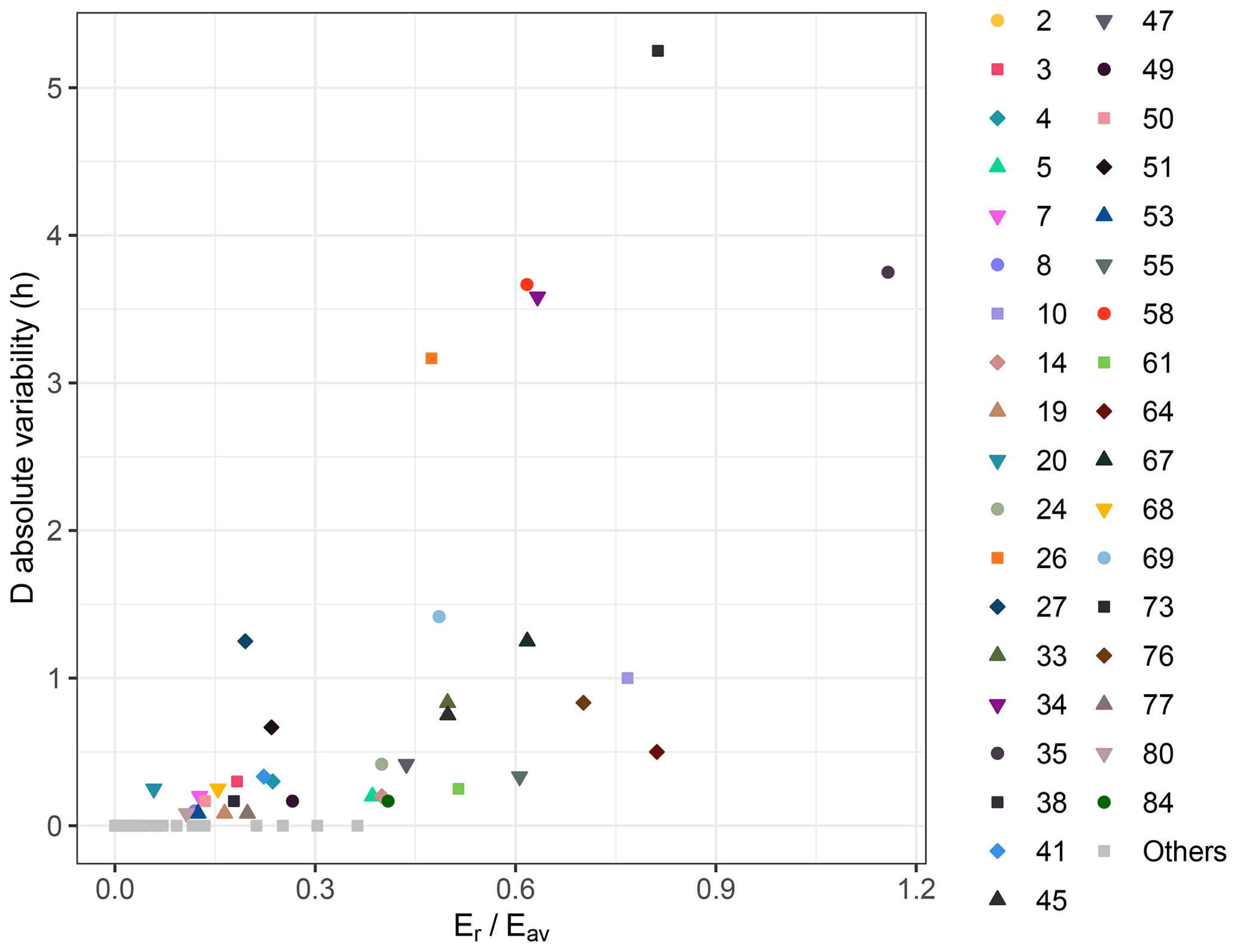
Figure 8Positive correlation between the absolute variability of D and , where Eav is the rainfall volume per unit area available in the main part of the hyetograph. The Spearman correlation coefficient is equal to 0.82 (). To make the graph clearer, the events with absolute variability of D equal to zero are represented with the same symbol.
5.2 Correlation between the D and I absolute variability and some event features
Despite the specificity of each considered event, it's possible to identify some event features that are correlated with the D and I absolute variability. It is worth noting that, in general, correlation does not imply causation (Wiedermann and Von Eye, 2016), but it is a starting point to understand if causality between the variables can be established.
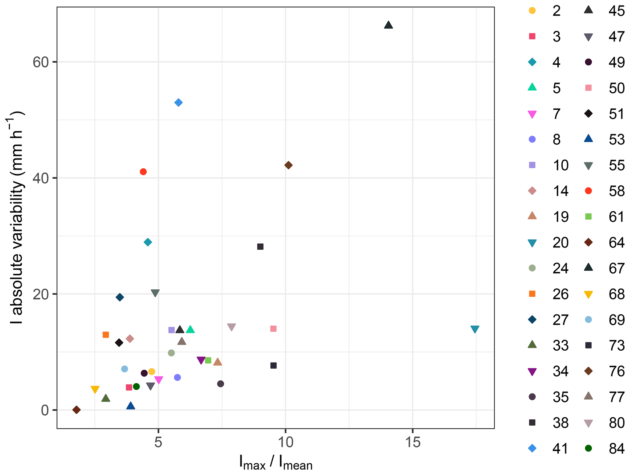
Figure 9Positive correlation between the non-null absolute variability of I and . Imax is the maximum intensity, and Imean is the mean intensity of the main part of the hyetograph. The Spearman correlation coefficient is equal to 0.48 (p=0.0035).
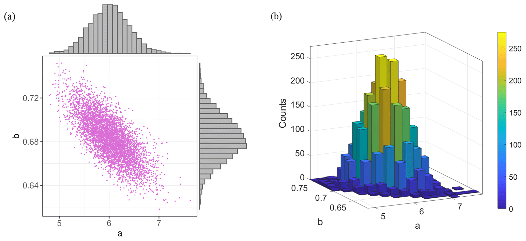
Figure 10Values a and b of Eq. (12) obtained performing 5000 MC simulations: (a) scatter plot and histogram and (b) 3D histogram.
We define Eav as the rainfall volume per unit area available in the “main part of the hyetograph”, namely the integral of the rainfall intensity on the smallest time interval comprising the peak and included between two instants with null intensities. We can then introduce the ratio . As shown in Fig. 8, the absolute variability of D and are positively correlated. A small value of means that the main part of the hyetograph is amply able to provide Er (i.e. to satisfy the condition of Eq. 8 in the reference conditions). This tends to avoid having to consider null intervals to achieve the values of E resulting from the MC simulation, namely to avoid D extremes. The opposite situation occurs if the ratio takes high values.
Regarding the intensity, we define Imax as the hyetograph maximum intensity and Imean as the mean intensity of the main part of the hyetograph for each event. The ratio provides a quantitative measure of the shape of the event hyetograph or, equivalently, of how impulsive the event is. As shown in Fig. 9, a positive correlation exists between the non-zero absolute variability of I and . If the shape of the hyetograph around the peak is flat, and the ratio is low, the variability of I, connected to the variability of D, is small since the average procedure, necessary to compute I, involves similar intensity intervals. The opposite occurs when the event is impulsive and the ratio is high. This consideration is valid only for events with non-zero absolute variability in I and D and tends to explain why some events with high variability in D have small variability in I (e.g. event 26).
5.3 Variability of the threshold
The result of the second MC simulation is 5000 (a,b) couples. The main statistical quantities of their distributions are given in Table 3. The relative variability is quantified through the CV that is equal to 6.46 % for a and 2.91 % for b. The low spread nature of a and b, highlighted by the small CV values, is also evident in the scatter plot and in the 3D histogram, respectively shown in Fig. 10a and b.
Table 3Mean, standard deviation, variation coefficient CV and mean 95 % confidence interval CI of the coefficients a and b of Eq. (12), computed by performing the second MC simulation.
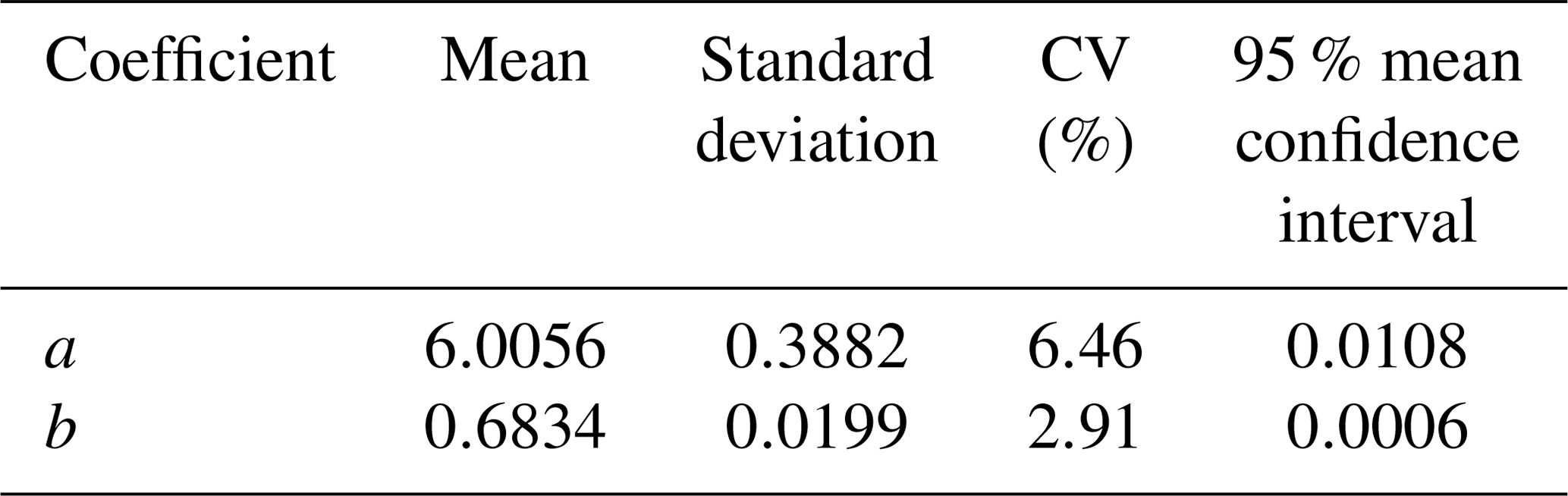
In addition, to analyse the absolute variability of the I–D threshold relation, the intensity values for each (a,b) couple are calculated for D values spanning from 5 min to 6 h with a 5 min time step. In this way, for each duration, we obtain an intensity distribution composed of 5000 samples. Then, the 2.5 and 97.5 percentiles of these distributions are chosen as upper and lower bounds of the threshold absolute variability. The result is shown in Fig. 11. According to the substantially symmetrical distributions of a and b (Fig. 10a), the threshold computed with the mean values of a and b (Table 3) is essentially equidistant from the lower and upper bounds. The variability bandwidth decreases monotonically by increasing the duration and varies between 5.61 and 0.64 mm h−1.
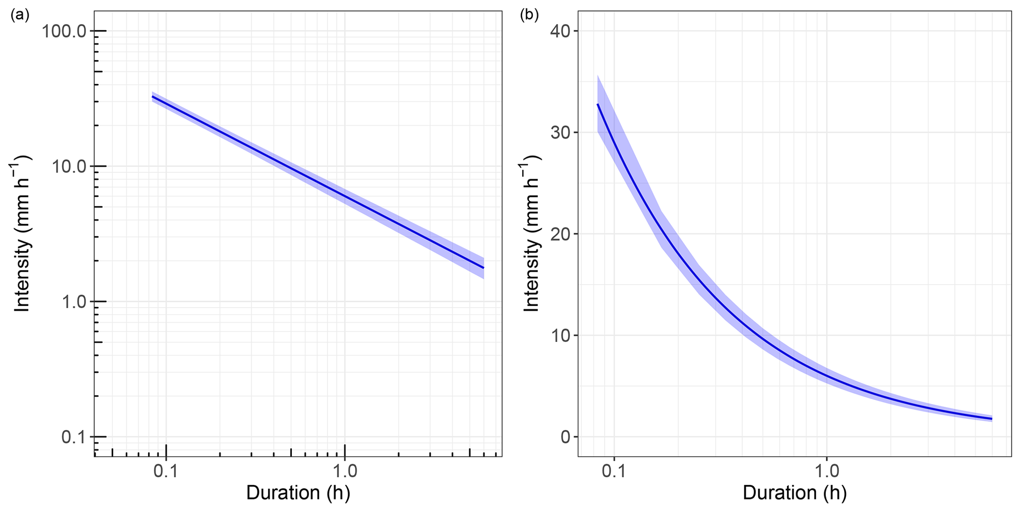
Figure 11(a) Log–log and (b) semi-log plot of the threshold absolute variability. The blue line is the rainfall threshold obtained using the mean value of a and b (Table 3). The shaded area represents the threshold absolute variability whose upper and lower bounds have been computed considering the 2.5 and 97.5 percentiles of the intensity distributions for fixed durations.
Hence, both the relative and the absolute variability highlight that the effect of the uncertainty in the variables on the threshold estimate is small. This is mainly due to the zero variability in the D and I distributions of 48 events out of 84: since the (I,D) points of these events are located in the same positions in all the 5000 MC simulations, they propagate zero uncertainty in the threshold computation.
5.4 Reference values versus MC means
Finally, a comparison between the results of the first and second MC simulation and the reference values is carried out. In particular, we compare
-
the means of the D and I distributions (Fig. 6) to the corresponding reference ones, for each event;
-
the mean threshold (i.e. threshold computed with the mean values of a and b) and the threshold absolute variability bounds (Fig. 11) to the reference threshold (i.e. Eq. 13).
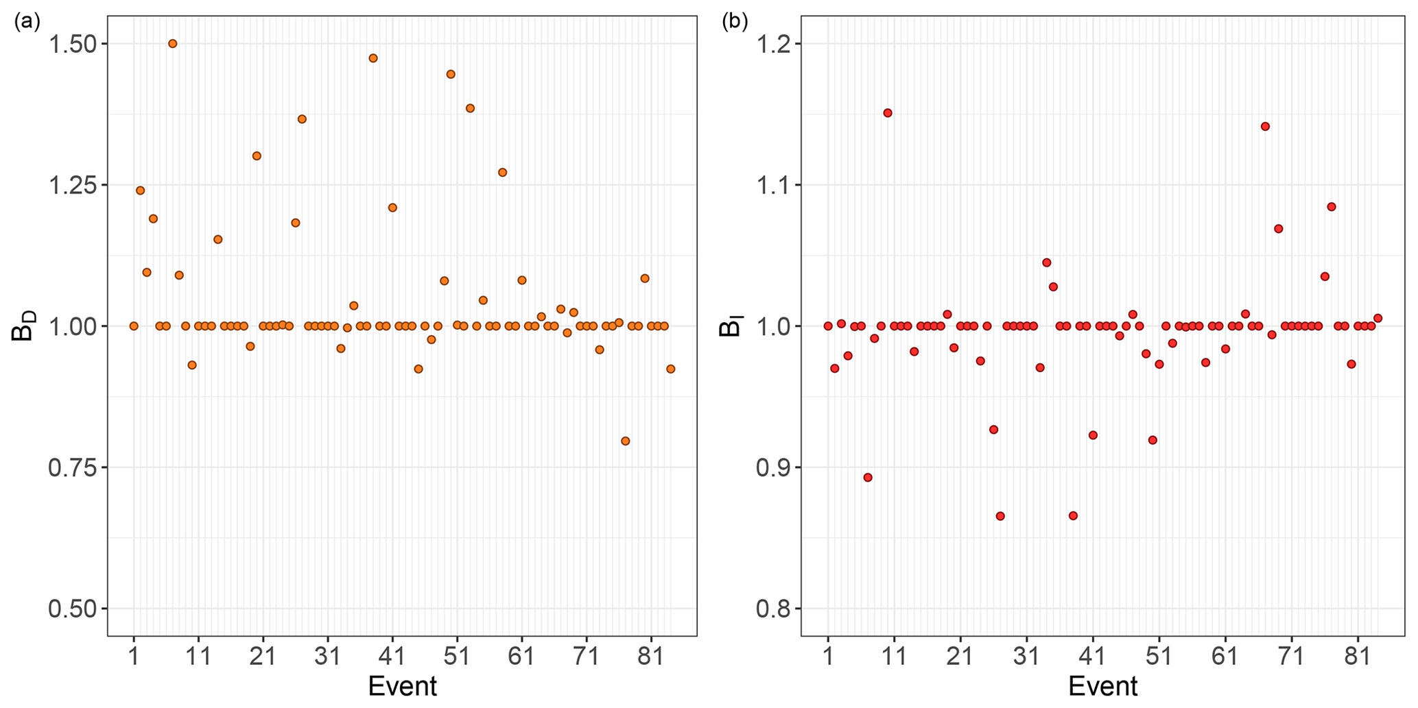
Figure 12Bias of (a) duration BD and (b) intensity BI between the mean values of the D and I distributions obtained performing the first MC simulation and the corresponding reference values for each event.
As regards D and I, according to Marra (2019), the bias of the duration BD and the intensity BI are computed for each event as
where the subscripts m represent the mean of the MC D and I distributions. The result is shown in Fig. 12: BD deviates between 0.8 and 1.5 (Fig. 12a), while BI deviates between 0.86 and 1.15 (Fig. 12b). Consistently with the variability analysis described in Sect. 5.1, most events (48) are characterised by . This means that for these zero-variability events, the reference duration and intensity are exactly the MC mean values of I and D, namely the only MC (I,D) couple. Moreover, most of the remaining events have BD>1 and BI<1. This signifies that the MC (I,D) mean couples tend to be located lower and more to the right than the reference ones in the log–log I–D plane.
Regarding the threshold, the differences between the MC intensities IMC,k, where k stands for mean, upper bound and lower bound, and the reference threshold ones It,r are carried out for the same durations used to define the absolute variability of the threshold:
The result is shown in Fig. 13a. For almost all durations, the intensities of the mean threshold are slightly lower than the reference threshold ones: a positive difference occurs only for the first time interval. Consistently with the obtained a and b mean values (Table 3) and the BD and BI trends, in the log–log I–D plane the mean threshold is respectively slightly more downward translated and clockwise rotated than the reference one. Instead, the upper and lower bounds are respectively always higher and lower than the reference threshold.
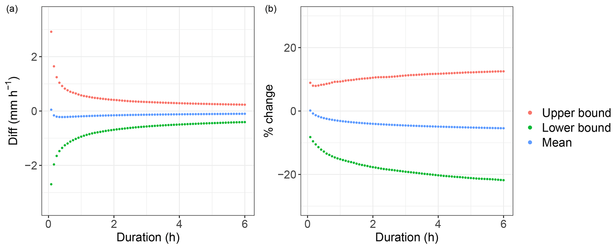
Figure 13(a) Difference between the MC intensities (upper bound, lower bound and mean) and the reference threshold ones as a function of the duration; (b) percentage change of the MC intensities with respect to the reference threshold ones, as a function of the duration.
Subsequently, the percentage changes, defined as
are computed to figure out how much the second MC outcomes deviate relatively from the reference threshold. The percentage changes are plotted in Fig. 13b: the mean threshold deviates between 0.14 % and −5.44 %, the upper bound between 8.06 % and 12.31 %, and the lower bound between −8.34 % and −22.94 % from the reference one.
It can therefore be generally stated that the outcomes of the uncertainty analyses, both (I,D) couples and threshold estimate, are consistent with the reference ones. Coherently with the previous analysis, also in this comparison, the duration is the quantity with the highest bias values. However, the mean threshold and the reference one are very close, pointing out the small effects of the differences between Dm and Dr on the threshold computation.
5.5 Further elements of uncertainty
In the calibration of the BDA-based threshold and in the assumptions of the developed method used to assess the uncertainty, it is possible to identify some elements that may introduce further uncertainty, beyond that considered in this analysis, in the calculation of the event characteristics and, consequently, in the estimate of the threshold. Firstly, the variability ranges and the probability distributions of the parameters and data, namely the uncertainty characterisation of the variables, are uncertain. Secondly, the equations of the BDA may be uncertain since they are based on some simplifications and hypothesis. Finally, the radar data may be affected by uncertainty due to other sources of error, beyond the beam shielding one (considered in this analysis), such as signal attenuation in heavy rain or wet radome attenuation (Marra et al., 2014). Nevertheless, at the present state of the research, it is not possible to assess the impact of these uncertainties on the event characteristics estimate, and further study is required.
This study has aimed to assess the effects of the uncertainty in the physical and morphological parameters and data on the BDA-based threshold calibration to evaluate the method robustness. To that end, a suitable methodology composed of two MC cascade simulations has been developed and applied to a specific study area and dataset. The first MC simulation has allowed examining the uncertainty propagation in the event characteristics estimate. The results have highlighted that most of the events (i.e 48 events out of 84) are characterised by zero variability in the estimation of the (I,D) couples, while the duration and the intensity related to the remaining events are affected by non-zero variability, which takes very different values depending on the event. Overall, the duration has found to be the most variable outcome in relative term while I, thanks to the average procedure, has a lower relative variability. In absolute terms, the variability of the (I,D) couples differs greatly between the events, and the D and I distributions tend to be skewed to the right and left respectively. Moreover, considering the mean values of the events with non-zero variability (36 events out of 84), the uncertainty in the variables tends to provide slightly longer durations and slightly smaller intensities with respect to the reference ones. Notwithstanding, the second MC simulation has shown that the threshold computation is affected by small variability. The low dispersion of the threshold coefficients is mainly due to the 48 events with zero variability. As a result, the BDA method, applied to the considered dataset, can be described as robust since it provides a calibrated threshold that is not as sensitive to the considered uncertainty in the parameters and data. This is also highlighted from the consistency between the uncertainty analysis mean threshold and the reference one.
Overall, the results of this analysis can be useful to calibrate a BDA-based threshold for a different study area since the investigation has highlighted the main elements that could undermine the BDA robustness. In particular, given a debris flow and the related rainfall event, it was noted that some event features are correlated with the variability of D and I. The percentage of the needed rainfall volume and the available one in the main part of the hyetograph is positively correlated with the absolute variability of D. Moreover, the shape of the main part of the hyetograph, described by the ratio between the maximum and the mean intensity, is positively correlated with the non-null absolute variability of I. Therefore, given an event, these trends can be used to presume the possible variability in the estimate of D and I, without carrying out a specific uncertainty analysis. In other words, if an event is characterised by (i) low availability of rainfall volume in the main part of the hyetograph with respect to the needed one and (ii) a peak intensity much greater than the mean one, variations in the parameters and data are likely to result in high variability in the D and I estimate. The presence of many events of this type could undermine the BDA robustness. Therefore, in these cases, it is advisable to put care in the estimate of the parameters and data.
Besides, given an event, further elements likely affecting the estimate of event characteristics have been highlighted in this study: (i) the variability ranges and the probability distributions of the parameters and data, (ii) the equations constituting the BDA model, and (iii) radar data. These elements can be affected by uncertainty and impact the event characteristics estimate. The uncertainty analysis performed in this study does not provide quantitative information on these impacts. Further analysis will assess how these three elements affect the (I,D) couple estimate and, consequently, the threshold calibration.
Moreover, the developed method, composed of two cascade MC simulations, can be applied to assess the uncertainty related to other threshold calibration approaches whose event characteristics estimate is based not only on the hyetograph but also on other variables (e.g. the one proposed by Zhang et al., 2020). Indeed, the developed method allows considering the entire range of uncertainty of the variables and, therefore, avoiding the analysis by scenarios, which are quite widespread in the literature for the uncertainty analysis of rainfall thresholds (e.g. Nikolopoulos et al., 2014; Peres et al., 2018). Analysing by scenarios may not be suitable if the uncertain parameters have a continuous range of variability. Indeed, a low number of input value combinations may not provide an overall assessment of the variability of the outputs.
Finally, it is worth noting that the results of this analysis are not useful to check the forecast capability of the threshold. Indeed, the variability in the threshold estimate due to the uncertainty of the inputs is not related to its forecast effectiveness but only to its robustness. The threshold forecast capability can be proved only by performing a proper validation analysis, which is essential to make this tool operational. Since the calibration method applied to the specific study area is proved to be robust, further analysis will assess the forecast capability of the threshold, developing an appropriate validation method.
The data used in this analysis are available upon request to the regional agencies of the Trentino-Alto Adige/Südtirol region.
MM designed the experiments, performed the analysis and wrote the paper. DZ and GR supervised the study, analysed the results and wrote the paper.
The authors declare that they have no conflict of interest.
This work has been carried out within the project “Progetto WEEZARD: un sistema integrato di modellazione matematica a servizio della sicurezza nei confronti di pericoli idrogeologici in ambiente montano” (CARITRO Foundation – Cassa di Risparmio di Trento e Rovereto). We thank Stefano Siboni for providing valuable suggestions and Ripartizione Opere Idrauliche and Ufficio Idrografico, Provincia Autonoma di Bolzano (Italy), and Servizio Bacini Montani and Ufficio Previsioni e Pianificazione, Provincia Autonoma di Trento (Italy), for supplying radar and debris-flow data.
This paper was edited by Filippo Catani and reviewed by two anonymous referees.
Abdi, H.: Coefficient of variation, Encyclopedia of Research Design, 1, 169–171, 2010. a
Abraham, M. T., Satyam, N., Rosi, A., Pradhan, B., and Segoni, S.: The Selection of Rain Gauges and Rainfall Parameters in Estimating Intensity-Duration Thresholds for Landslide Occurrence: Case Study from Wayanad (India), Water-SUI, 12, 1000, https://doi.org/10.3390/w12041000, 2020. a
Arachchige, C. N., Prendergast, L. A., and Staudte, R. G.: Robust analogs to the coefficient of variation, J. Appl. Stat., https://doi.org/10.1080/02664763.2020.1808599, in press, 2020. a
Baum, R. L. and Godt, J. W.: Early warning of rainfall-induced shallow landslides and debris flows in the USA, Landslides, 7, 259–272, 2010. a
Bendel, R., Higgins, S., Teberg, J., and Pyke, D.: Comparison of skewness coefficient, coefficient of variation, and Gini coefficient as inequality measures within populations, Oecologia, 78, 394–400, 1989. a
Bernard, M., Boreggio, M., Degetto, M., and Gregoretti, C.: Model-based approach for design and performance evaluation of works controlling stony debris flows with an application to a case study at Rovina di Cancia (Venetian Dolomites, Northeast Italy), Sci. Total Environ., 688, 1373–1388, 2019. a
Bisci, C., Fazzini, M., Dramis, F., Lunardelli, R., Trenti, A., and Gaddo, M.: Analysis of spatial and temporal distribution of precipitation in Trentino (Italian Eastern Alps): Preliminary Report, Meteorol. Z., 13, 183–187, 2004. a
Blijenberg, H.: In-situ strength tests of coarse, cohesionless debris on scree slopes, Eng. Geol., 39, 137–146, 1995. a
Brardinoni, F., Church, M., Simoni, A., and Macconi, P.: Lithologic and glacially conditioned controls on regional debris-flow sediment dynamics, Geology, 40, 455–458, 2012. a
Brunetti, M. T., Peruccacci, S., Rossi, M., Luciani, S., Valigi, D., and Guzzetti, F.: Rainfall thresholds for the possible occurrence of landslides in Italy, Nat. Hazards Earth Syst. Sci., 10, 447–458, https://doi.org/10.5194/nhess-10-447-2010, 2010. a
Caine, N.: The rainfall intensity-duration control of shallow landslides and debris flows, Geogr. Ann. A, 62, 23–27, 1980. a
Cánovas, J. B., Stoffel, M., Corona, C., Schraml, K., Gobiet, A., Tani, S., Sinabell, F., Fuchs, S., and Kaitna, R.: Debris-flow risk analysis in a managed torrent based on a stochastic life-cycle performance, Sci. Total Environ., 557, 142–153, 2016. a
Cepeda, J., Höeg, K., and Nadim, F.: Landslide-triggering rainfall thresholds: a conceptual framework, Q. J. Eng. Geol. Hydroge., 43, 69–84, 2010. a
Chau, T., Young, S., and Redekop, S.: Managing variability in the summary and comparison of gait data, J. Neuroeng. Rehabil., 2, 1–20, 2005. a
Chien-Yuan, C., Tien-Chien, C., Fan-Chieh, Y., Wen-Hui, Y., and Chun-Chieh, T.: Rainfall duration and debris-flow initiated studies for real-time monitoring, Environ. Geol., 47, 715–724, 2005. a
Coleman, H. W. and Steele, W. G.: Experimentation, validation, and uncertainty analysis for engineers, John Wiley & Sons, New York, 2018. a
Dowling, C. A. and Santi, P. M.: Debris flows and their toll on human life: a global analysis of debris-flow fatalities from 1950 to 2011, Nat. Hazards, 71, 203–227, 2014. a
Frattini, P., Crosta, G., and Sosio, R.: Approaches for defining thresholds and return periods for rainfall-triggered shallow landslides, Hydrol. Process., 23, 1444–1460, 2009. a
Fuchs, S., Keiler, M., Sokratov, S., and Shnyparkov, A.: Spatiotemporal dynamics: the need for an innovative approach in mountain hazard risk management, Nat. Hazards, 68, 1217–1241, 2013. a
Gariano, S. L., Melillo, M., Peruccacci, S., and Brunetti, M. T.: How much does the rainfall temporal resolution affect rainfall thresholds for landslide triggering?, Nat. Hazards, 100, 655–670, https://doi.org/10.1007/s11069-019-03830-x, 2020. a, b
Germann, U., Galli, G., Boscacci, M., and Bolliger, M.: Radar precipitation measurement in a mountainous region, Q. J. Roy. Meteor. Soc., 132, 1669–1692, 2006. a
Giannecchini, R.: Rainfall triggering soil slips in the southern Apuan Alps (Tuscany, Italy), Advances in Geosciences, 2, 21–24, 2005. a
Giannecchini, R., Galanti, Y., Avanzi, G. D., and Barsanti, M.: Probabilistic rainfall thresholds for triggering debris flows in a human-modified landscape, Geomorphology, 257, 94–107, 2016. a
Guzzetti, F., Peruccacci, S., Rossi, M., and Stark, C. P.: Rainfall thresholds for the initiation of landslides in central and southern Europe, Meteorol. Atmos. Phys., 98, 239–267, 2007. a
Guzzetti, F., Peruccacci, S., Rossi, M., and Stark, C. P.: The rainfall intensity–duration control of shallow landslides and debris flows: an update, Landslides, 5, 3–17, 2008. a
Håkanson, L.: The role of characteristic coefficients of variation in uncertainty and sensitivity analyses, with examples related to the structuring of lake eutrophication models, Ecol. Model., 131, 1–20, 2000. a
Helton, J. C., Johnson, J. D., Sallaberry, C. J., and Storlie, C. B.: Survey of sampling-based methods for uncertainty and sensitivity analysis, Reliab. Eng. Syst. Safe., 91, 1175–1209, 2006. a, b
Hofer, E.: The Uncertainty Analysis of Model Results, Springer International Publishing, Cham, 2018. a
Huebl, J. and Fiebiger, G.: Debris-flow mitigation measures, in: Debris-flow hazards and related phenomena, Springer, Berlin, Heidelberg, 445–487, 2005. a
Iadanza, C., Trigila, A., and Napolitano, F.: Identification and characterization of rainfall events responsible for triggering of debris flows and shallow landslides, J. Hydrol., 541, 230–245, 2016. a
Jakob, M., Owen, T., and Simpson, T.: A regional real-time debris-flow warning system for the District of North Vancouver, Canada, Landslides, 9, 165–178, 2012. a
Lane, E. W.: Progress report on studies on the design of stable channels of the Bureau of Reclamation, Proc. Am. Soc. Civ. Eng., 79, 246–261, 1953. a
Li, T.-T., Huang, R.-Q., and Pei, X.-J.: Variability in rainfall threshold for debris flow after Wenchuan earthquake in Gaochuan River watershed, Southwest China, Nat. Hazards, 82, 1967–1980, 2016. a
Marchi, L., Brunetti, M. T., Cavalli, M., and Crema, S.: Debris-flow volumes in northeastern Italy: Relationship with drainage area and size probability, Earth Surf. Proc. Land., 44, 933–943, 2019. a
Marino, S., Hogue, I. B., Ray, C. J., and Kirschner, D. E.: A methodology for performing global uncertainty and sensitivity analysis in systems biology, J. Theor. Biol., 254, 178–196, 2008. a, b
Marra, F.: Rainfall thresholds for landslide occurrence: systematic underestimation using coarse temporal resolution data, Nat. Hazards, 95, 883–890, 2019. a, b
Marra, F., Nikolopoulos, E. I., Creutin, J. D., and Borga, M.: Radar rainfall estimation for the identification of debris-flow occurrence thresholds, J. Hydrol., 519, 1607–1619, 2014. a, b
Marra, F., Nikolopoulos, E. I., Creutin, J. D., and Borga, M.: Space–time organization of debris flows-triggering rainfall and its effect on the identification of the rainfall threshold relationship, J. Hydrol., 541, 246–255, 2016. a
McKay, M. D., Beckman, R. J., and Conover, W. J.: A comparison of three methods for selecting values of input variables in the analysis of output from a computer code, Technometrics, 42, 55–61, 2000. a
Nikolopoulos, E. I., Crema, S., Marchi, L., Marra, F., Guzzetti, F., and Borga, M.: Impact of uncertainty in rainfall estimation on the identification of rainfall thresholds for debris flow occurrence, Geomorphology, 221, 286–297, 2014. a, b, c, d
Oberkampf, W. L., Helton, J. C., Joslyn, C. A., Wojtkiewicz, S. F., and Ferson, S.: Challenge problems: uncertainty in system response given uncertain parameters, Reliab. Eng. Syst. Safe., 85, 11–19, 2004. a
Pan, H.-L., Jiang, Y.-J., Wang, J., and Ou, G.-Q.: Rainfall threshold calculation for debris flow early warning in areas with scarcity of data, Nat. Hazards Earth Syst. Sci., 18, 1395–1409, https://doi.org/10.5194/nhess-18-1395-2018, 2018. a
Peres, D. J., Cancelliere, A., Greco, R., and Bogaard, T. A.: Influence of uncertain identification of triggering rainfall on the assessment of landslide early warning thresholds, Nat. Hazards Earth Syst. Sci., 18, 633–646, https://doi.org/10.5194/nhess-18-633-2018, 2018. a, b
Peruccacci, S., Brunetti, M. T., Luciani, S., Vennari, C., and Guzzetti, F.: Lithological and seasonal control on rainfall thresholds for the possible initiation of landslides in central Italy, Geomorphology, 139, 79–90, 2012. a
Prancevic, J. P. and Lamb, M. P.: Unraveling bed slope from relative roughness in initial sediment motion, J. Geophys. Res.-Earth, 120, 474–489, 2015. a
R Core Team: R: A Language and Environment for Statistical Computing, R Foundation for Statistical Computing, Vienna, Austria, http://www.R-project.org/ (last access: 2 February 2021), 2013. a
Rosatti, G., Zugliani, D., Pirulli, M., and Martinengo, M.: A new method for evaluating stony debris flow rainfall thresholds: the Backward Dynamical Approach, Heliyon, 5, e01994, https://doi.org/10.1016/j.heliyon.2019.e01994, 2019. a, b, c, d, e
Rossi, M., Luciani, S., Valigi, D., Kirschbaum, D., Brunetti, M., Peruccacci, S., and Guzzetti, F.: Statistical approaches for the definition of landslide rainfall thresholds and their uncertainty using rain gauge and satellite data, Geomorphology, 285, 16–27, 2017. a
Segoni, S., Piciullo, L., and Gariano, S. L.: A review of the recent literature on rainfall thresholds for landslide occurrence, Landslides, 15, 1483–1501, 2018. a, b, c, d, e
Staley, D. M., Kean, J. W., Cannon, S. H., Schmidt, K. M., and Laber, J. L.: Objective definition of rainfall intensity–duration thresholds for the initiation of post-fire debris flows in southern California, Landslides, 10, 547–562, 2013. a
Stancanelli, L., Lanzoni, S., and Foti, E.: Propagation and deposition of stony debris flows at channel confluences, Water Resour. Res., 51, 5100–5116, 2015. a
Takahashi, T.: Mechanical characteristics of debris flow, J. Hydr. Eng. Div.-ASCE, 104, 1153–1169, 1978. a
Takahashi, T.: A review of Japanese debris flow research, International Journal of Erosion Control Engineering, 2, 1–14, 2009. a
Takahashi, T.: Debris flow: mechanics, prediction and countermeasures, CRC Press, London, 2014. a
Uijlenhoet, R.: Raindrop size distributions and radar reflectivity–rain rate relationships for radar hydrology, Hydrol. Earth Syst. Sci., 5, 615–628, https://doi.org/10.5194/hess-5-615-2001, 2001. a
Wiedermann, W. and Von Eye, A.: Statistics and causality, John Wiley & Sons, Hoboken, New Jersey, 2016. a
Winter, M., Dent, J., Macgregor, F., Dempsey, P., Motion, A., and Shackman, L.: Debris flow, rainfall and climate change in Scotland, Q. J. Eng. Geol. Hydroge., 43, 429–446, 2010. a
Zhang, S. J., Xu, C. X., Wei, F. Q., Hu, K. H., Xu, H., Zhao, L. Q., and Zhang, G. P.: A physics-based model to derive rainfall intensity-duration threshold for debris flow, Geomorphology, 351, 2020. a
Zhou, W. and Tang, C.: Rainfall thresholds for debris flow initiation in the Wenchuan earthquake-stricken area, southwestern China, Landslides, 11, 877–887, 2014. a