the Creative Commons Attribution 4.0 License.
the Creative Commons Attribution 4.0 License.
 | 03 Jun 2021
Spatially compounded surge events: an example from hurricanes Matthew and Florence
Kelley DePolt
Jamie Kruse
Anuradha Mukherji
Jennifer Helgeson
Ausmita Ghosh
Philip Van Wagoner
The simultaneous rise of tropical-cyclone-induced flood waters across a large hazard management domain can stretch rescue and recovery efforts. Here we present a means to quantify the connectedness of maximum surge during a storm with geospatial statistics. Tide gauges throughout the extensive estuaries and barrier islands of North Carolina deployed and operating during hurricanes Matthew (n=82) and Florence (n=123) are used to compare the spatial compounding of surge for these two disasters. Moran's I showed the occurrence of maximum storm tide was more clustered for Matthew compared to Florence, and a semivariogram analysis produced a spatial range of similarly timed storm tide that was 4 times as large for Matthew than Florence. A more limited data set of fluvial flooding and precipitation in eastern North Carolina showed a consistent result – multivariate flood sources associated with Matthew were more concentrated in time as compared to Florence. Although Matthew and Florence were equally intense, they had very different tracks and speeds which influenced the timing of surge along the coast.
- Article
(4373 KB) - Full-text XML
- BibTeX
- EndNote


1.1 Spatially compounded weather events
Compound climate and weather events have been defined as the “combination of multiple drivers and hazards that contributes to societal or environmental risk” (Zscheischler et al., 2018), undermining hazard management (Raymond et al., 2020). For example, emergency managers and planners often use tools that only consider one hazard to estimate risk, whereas the combination of hazards leads to a nonlinear increase in risk (Moftakhari et al., 2017). This underestimation of risk leads to under-resourcing for prevention prior to an event and the adoption of extra measures for recovery once the risk is realized. Also, the complex nature of compound hazards in time and space during an event may stretch first responders to capacity. Thus, the entire emergency management cycle of response, recovery, mitigation, and preparedness needs to be reframed in the context of compounded hazards (Raymond et al., 2020).
Zscheischler et al. (2020) expanded the typology of compound weather and climate events to include four themes: preconditioned, multivariate, temporally compounding, and spatially compounding. They also include a modulator to the definition, which is a state of the atmosphere or climate, such as a climatic teleconnection, stationary weather pattern, or storm that increases the probability of the drivers. The present study adds to our understanding of the spatially compounding event type, which Zscheischler et al. (2020) define as “multiple-connected locations affected by the same or different hazards, within a limited time window, thereby causing an impact”. Spatially compounded events can restrict emergency response actions if the operational space (jurisdiction) experiences coincidental hazards (Leonard et al., 2014). This can lead to a disaster situation, as about 50 % of deaths typically occur within a few hours after an event (Narayanan and Ibe, 2012). Thus, the temporal component is an important consideration.
Several studies have used spatial statistics to better understand compounded hazards, mostly on a national scale. For example, Touma et al. (2018) used the semivariogram to characterize length scales of extreme daily precipitation (90th percentile) in the US. This analysis was refined to determine the spatial extent of extreme precipitation during the evolution of landfalling tropical cyclones (Touma et al., 2019). Du et al. (2020) used a rotating calipers algorithm to quantify the spatial scales of heavy Meiyu precipitation events, and Blanchet and Creutin (2017) modeled the probability of co-occurrence of extreme precipitation in the French Mediterranean region with the Brown–Resnick max-stable process. More recently the connectedness of fluvial flooding has been examined using the F-madogram (Brunner et al., 2020). While these studies provide important climatological information that will inform pluvial and fluvial flood risk, the current study analyzes another flood hazard – storm surge – and defines the spatially aggregate impacts within an individual storm.
Storm surge – or the rise of coastal waters generated by storm winds and severe drop in atmospheric pressure – is the greatest threat from tropical cyclones globally (NHC, 2020). In the US this hazard amounted to almost half of hurricane fatalities between 1963 and 2012 as people either could not or would not evacuate (Rappaport, 2014). Evacuation can become problematic in a spatially compounded event with the simultaneous inundation of roadways and railways within a region (Koks et al., 2019; Zscheischler et al., 2020). The goal of this study is to quantify the spatially compounded surge hazard over a large geographic area via two contrasting tropical cyclone cases, both of which had a severe impact on the US: Hurricane Matthew, which made landfall south of McClellanville, South Carolina (SC), as a category 1 storm at 15:00 UTC on 8 October 2016; and Hurricane Florence, which made landfall approximately 250 km to the northeast at Wrightsville Beach, North Carolina (NC), also a category 1 storm at the time, at 11:15 UTC on 14 September 2018. Eastern North Carolina (Fig. 1) is the focus of our study for a number of reasons. Firstly, Matthew and Florence caused more direct fatalities in North Carolina than any other state. Secondly, North Carolina has a large estuary system and extensive inhabited barrier island complex comprising 17 152 km of shoreline, which complicates evacuation and rescue operations during storm surge but is conducive to a spatial analysis. Finally, this study is part of a larger project related to compound flood risk and management in rural eastern North Carolina.

Figure 1Orientation map of North Carolina counties that fall within the eastern branch of the North Carolina Department of Emergency Management. © OpenStreetMap contributors 2020. Distributed under a Creative Commons BY-SA License.
1.2 Hurricanes Matthew and Florence
According to the National Hurricane Center's (NHC) cyclone reports, hurricanes Matthew and Florence were the 10th and 9th most destructive storms in the US (Stewart, 2017; Stewart and Berg, 2019). In North Carolina alone, Matthew caused USD 1.5 billion in property damage, while Florence caused USD 22 billion. However, Matthew caused more direct fatalities in the state (25) as compared to Florence (15). Casualties and damages were primarily attributed to pluvial and fluvial flooding and storm surge. Thus, these storms would be appropriately categorized as multivariate compound events (Zscheischler et al., 2020). However, Zscheischler et al. (2020) recognize that their defined typology has soft boundaries and that events can fall into multiple categories. Figure 2a shows the track of Hurricane Matthew. The storm paralleled the study area from 18:00 UTC on 8 October 2016 and exited off the coast of North Carolina around 09:00 UTC on 9 October (∼15 h in total). During this time much of the coast experienced winds greater than 26 m s−1 (50 kn). Matthew's highest recorded storm surge in North Carolina was 1.76 m above mean highest high water (MHHW) on Hatteras Island (Stewart, 2017). Hurricane Florence's track (Fig. 2b) was nearly perpendicular to Matthew's as the storm approached the coast at 00:00 UTC on 14 September 2018 from the east and exited the study area around 00:00 UTC on 15 September (∼24 h in total). During Florence's passage through the study area wind speeds diminished from hurricane force in the south to tropical storm force in the north (Fig. 2b). Florence then turned northward and became a post-tropical cyclone. The last NHC report located its center at 42.6∘ N and 71.9∘ W (near Boston, MA) at 15:00 UTC on 18 September. The storm was elongated so at this time southeasterly winds were observed in the northern portion of the study area. Florence's highest recorded storm surge in North Carolina was 3.17 m above MHHW near New Bern (Stewart and Berg, 2019).
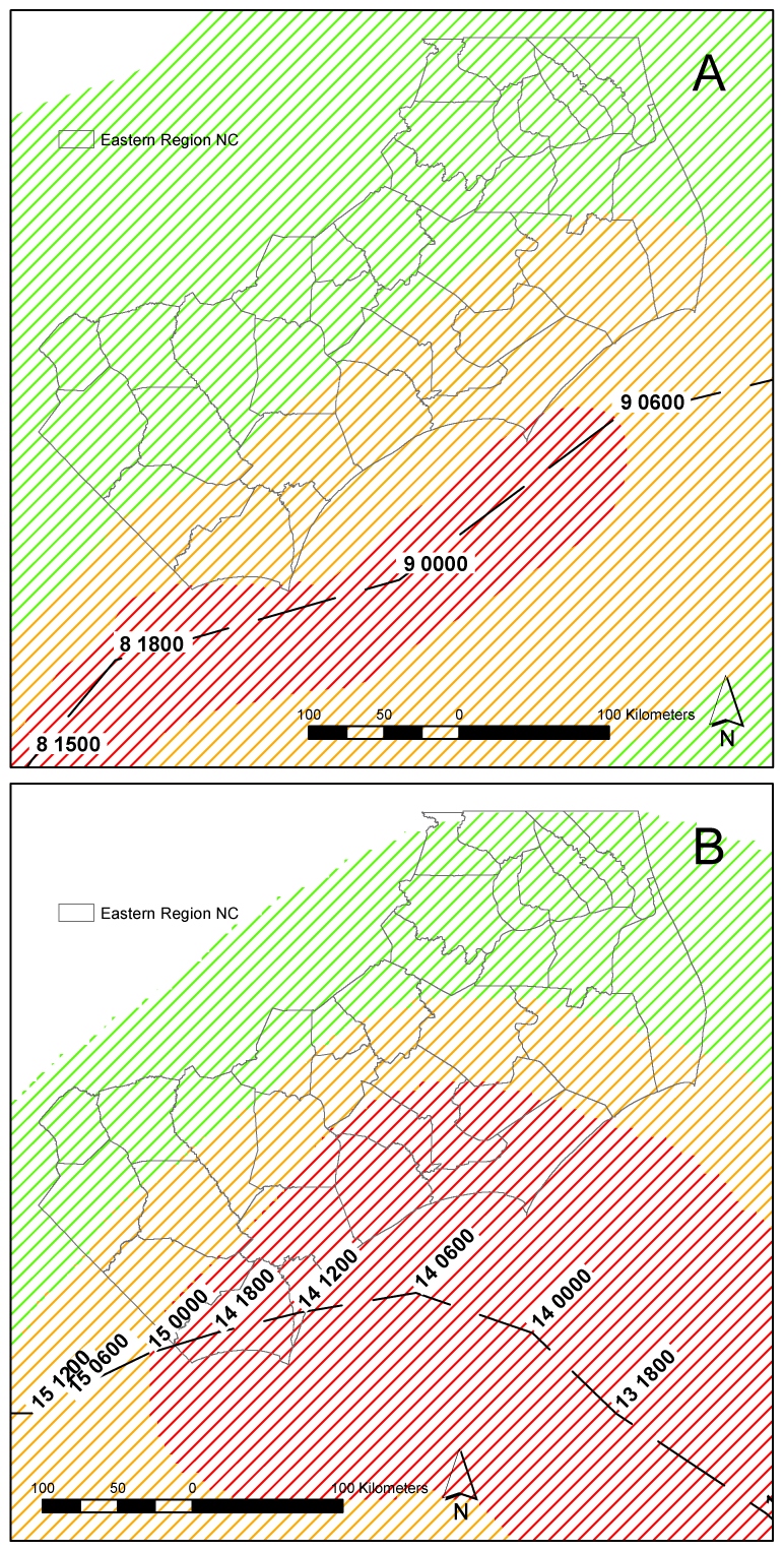
Figure 2Track and wind speeds during the passage of hurricanes (a) Matthew and (b) Florence off the coast of North Carolina. Red stippling indicates hurricane force winds (>33 m s−1), orange storm force (>26 m s−1), and green tropical storm force (>17 m s−1). The track is denoted by the dashed line. The first number is the day, and the second number is the time (UTC) in October 2016 for (a) and September 2018 for (b).
Storm tide data for hurricanes Matthew and Florence were collected from the US Geologic Survey (USGS) Flood Event Viewer (https://stn.wim.usgs.gov/FEV/, last access: 1 June 2021). Flood Event Viewer provides a file of locational data for all tidal stations – rapid deployment and pressure transducers – in operation during significant weather events. For Hurricane Florence a peak summary file was also available, which includes the unfiltered peak water level recorded in feet above NAVD88 and the time of the recording. Matthew did not have such a summary, so these attributes were manually recorded from each sensor's page and appended to the locational data. Heights were converted to meters, and data from outside North Carolina were removed. Some of the stations in the peak summary file had an initial storm-tide-related value and a subsequent river runoff value. Only the surge information was retained. The final number of peak storm tides in North Carolina after a quality control was 82 for Matthew and 123 for Florence.
To understand how an event is spatially compounded requires quantifying either the spatial extent over a predefined time interval or the temporal extent over a predefined spatial domain. An example of the former definition would be delineating roadways impacted by flooding over the duration of the storm. However, characterizing the capacity of emergency responders to perform their job within a set jurisdiction would fall under the later definition. It is argued that if peak storm tide occurs simultaneously within the jurisdiction, it would stretch the ability of search and rescue teams, such as Swiftwater, part of the North Carolina Division of Emergency Management (NCDEM). The tide gauge data collected for both storms fall under the eastern branch of the NCDEM (see Fig. 1 for boundary). To complement the tide gauge analysis over the defined spatial domain, we obtained other indicators of flooding that were operational during Matthew and Florence, namely 10 USGS stream gauges that had defined flooding thresholds and two US National Centers for Environmental Information 15 min rain gauges. It is assumed that the geographic extent of surge flooding will be greatest at the time the tide gauge is at its maximum. To compare the temporal evolution of peak surge across storms requires a reference time. Here we selected the time of landfall: 08:00 UTC on 9 October 2016 for Matthew and 11:15 UTC on 14 September 2018 for Florence. Differences between time of peak surge and landfall (Δtps-lf) were calculated in days and added to the peak surge tables.
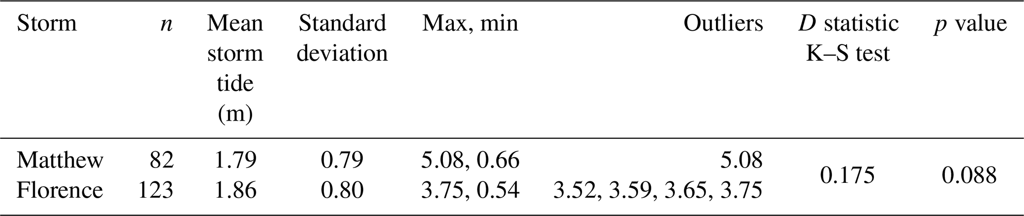
Table 1Basic statistics on North Carolina peak storm tide during hurricanes Matthew and Florence. A measure of the difference in the distributions is given with the Kolmogorov–Smirnov D statistic. The significance level is denoted by the p value.
A Kolmogorov–Smirnov (K–S) test was used to determine if the distributions of (i) maximum tide magnitudes and (ii) their timings (Δtps-lf) between the Matthew (n=82) and Florence (n=123) tide records were significantly different. The D statistic is calculated as the maximum difference between two cumulative distributions, and :
Next, two tests were performed in ArcGIS to understand the spatial correlation of Δtps-lf: global Moran's I and the range of the semivariogram function. Moran's I is an inferential statistic, for which the null hypothesis is that a variable x, here x=Δtps-lf, is randomly distributed throughout a spatial range:
where z is the deviation of x from its mean, wi,j is the spatial weight between xi and xj, and n is the total number of tide gauge stations. So is the sum of all spatial weights:
An expected Moran's I is computed and compared to the observed value to generate a z score and p value for significance testing. A significantly positive (negative) value of Moran's I would suggest that the variable x is clustered (dispersed). A Moran's I test has been used previously to determine the spatial clustering of precipitation within the Gulf of Mexico during phases of the El Niño–Southern Oscillation (Munroe et al., 2014). Next, we follow the procedure of Touma et al. (2018, 2019) and use the semivariogram to test the hypothesis that variables closer in space would be more similar than those far apart. Thus, the raw semivariogram is a function of distance h between variables xi and xj and is simply half the variance or
The data can then be modeled statistically with a family of functions. The most appropriate fitted semivariogram for our data was provided by the following stable model:
where Co is the sill of the semivariogram, s is the shape parameter, a is the range, and b is the nugget. We experimented with other functions, but it was discovered that over half produced unphysical results, while the others yielded the same basic results as the stable model. An added advantage of the stable model is the shape parameter, s, which transforms the function to be more like an exponential or spherical model when and more like a Gaussian model when s>2. In this study we are particularly interested in the range, a, as this is when the spatial autocorrelation first becomes negligible. Thus, the range gives an indication of spatial scale for coincidental storm surge.
Table 1 gives some basic statistics for storm surge peak magnitude. In this data set Matthew had the largest storm tide at 5.08m recorded at a pressure transducer (NCDAR12768) at the Sanderling Resort (Atlantic coast of Dare County). However, Florence had more outlier peak storm tides in excess of 3.5 m. Both storms had similar means and standard deviations. The D statistic between the two storms was 0.175, which did not reach the 0.05 significance level, so the distributions cannot be considered different (Table 1).
Interestingly, the distribution of Δtps-lf was very different between Matthew and Florence (Table 2). Both storms had mean peak storm tide at less than 1 d after landfall (10–14 h). However, the standard deviation of Δtps-lf was less than the mean for Matthew (0.34 d) but more than double the mean for Florence (1.29 d). There were seven outliers in the Florence record from 3.53 d to a maximum of 7.33 d. It is not surprising then that the D statistic between the two storms was 0.309 and highly significant. Histograms of Δtps-lf in 15 min increments are given in Fig. 3a. As suggested from Table 2, Matthew's peak storm tide was clustered in time, with 66 % occurring within the first 12 h after landfall. Only 37 % of Florence's peak surge occurred during this critical time.
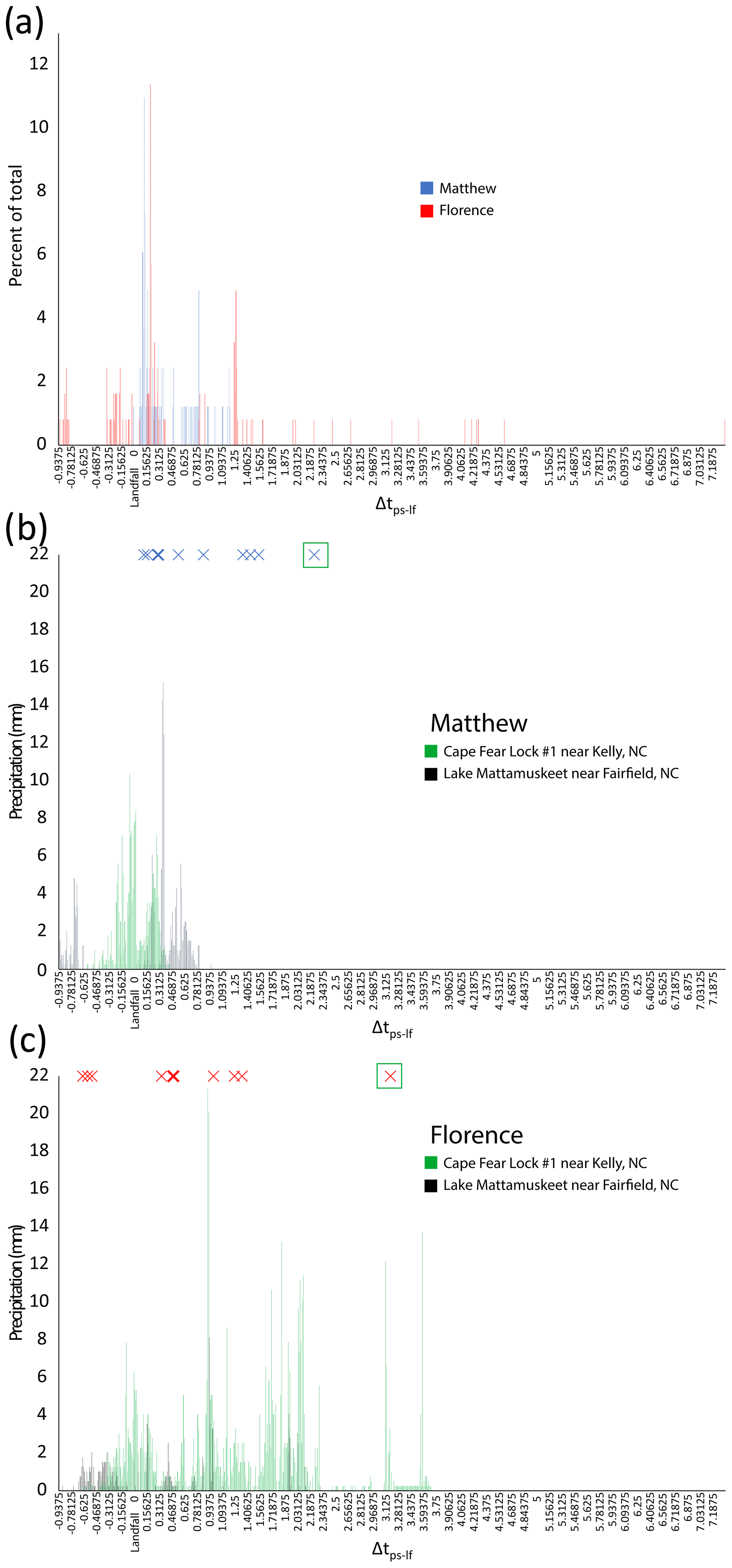
Figure 3Time evolution of surge, rainfall, and river flooding during hurricanes Matthew and Florence in North Carolina. X axis is Δtps-lf binned in 15 min increments (unit days) and covers approximately 1 d prior to landfall to 7 d after. (a) Percent of peak surge occurrences; blue is for Matthew, and red is for Florence. Panels (b) and (c) display precipitation (mm) and initial fluvial flooding in the same 15 min increments during Matthew and Florence respectively. Green bars represent precipitation recorded at the Cape Fear Lock #1 rain gauge near Kelly, NC, and black bars represent precipitation recorded at the Lake Mattamuskeet rain gauge near Fairfield, NC. Crosses indicate when river gauges in the study area first reached minor flood stage. Bold crosses represent two river gauges reaching minor flood stage in the same 15 min increment. Cross bounded by green square is the river gauge co-located with the Cape Fear Lock #1 rain gauge.
Table 2Basic statistics on the difference in time (days) between peak storm tide in North Carolina and landfall (Δtps-lf) for hurricanes Matthew and Florence. A measure of the difference in the distributions is given with the Kolmogorov–Smirnov D statistic. Significance level is denoted by the p value.
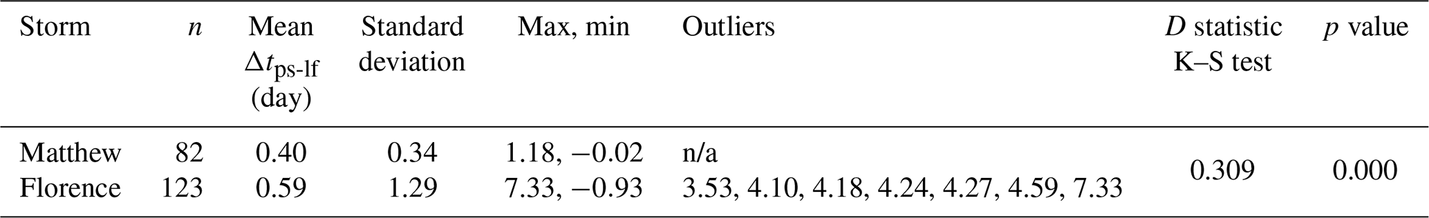
n/a stands for not applicable.
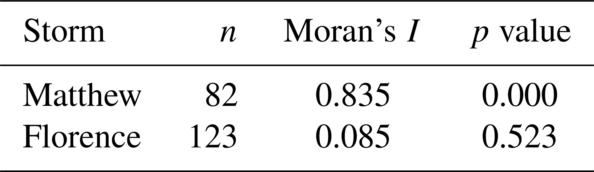
Complementary to the difference in the distribution of Δtps-lf between Matthew and Florence, the Moran's I test (Table 3) shows that for Matthew Δtps-lf was significantly clustered in space, equating to a spatially compounded event, whereas the insignificance of Moran's I for Florence indicates random spatial distribution. Values of Δtps-lf along coastal North Carolina for the two storms are shown as circles in Fig. 4. For Matthew there is very little difference in Δtps-lf geographically, although some of the later values appear to occur on the Outer Banks in Dare County (see Fig. 1 for reference). In the case of Florence (Fig. 4b), from pre-landfall to 1.5 d after there appears to be a north to south gradient in Δtps-lf. The earliest peaks, taking place before landfall, occurred on the Outer Banks and the mid-region of Beaufort, Pamlico, and Carteret counties (see Fig. 1 for reference). Peaks that occurred between 0 and 1.5 d after landfall are generally found along the southeastern coast – Onslow, Pender, New Hanover, and Brunswick counties. However, peaks occurring 1.5 to 2.5 d after landfall appear in the north region of Bertie, Washington, and Tyrrell counties with some values near Cape Hatters in Dare County. Δtps-lf on the order of 3–4 d can be found even further north in Pasquotank, Perquimans, and Currituck counties. Finally, the maximum Δtps-lf of over 7 d is seen in New Hanover County.
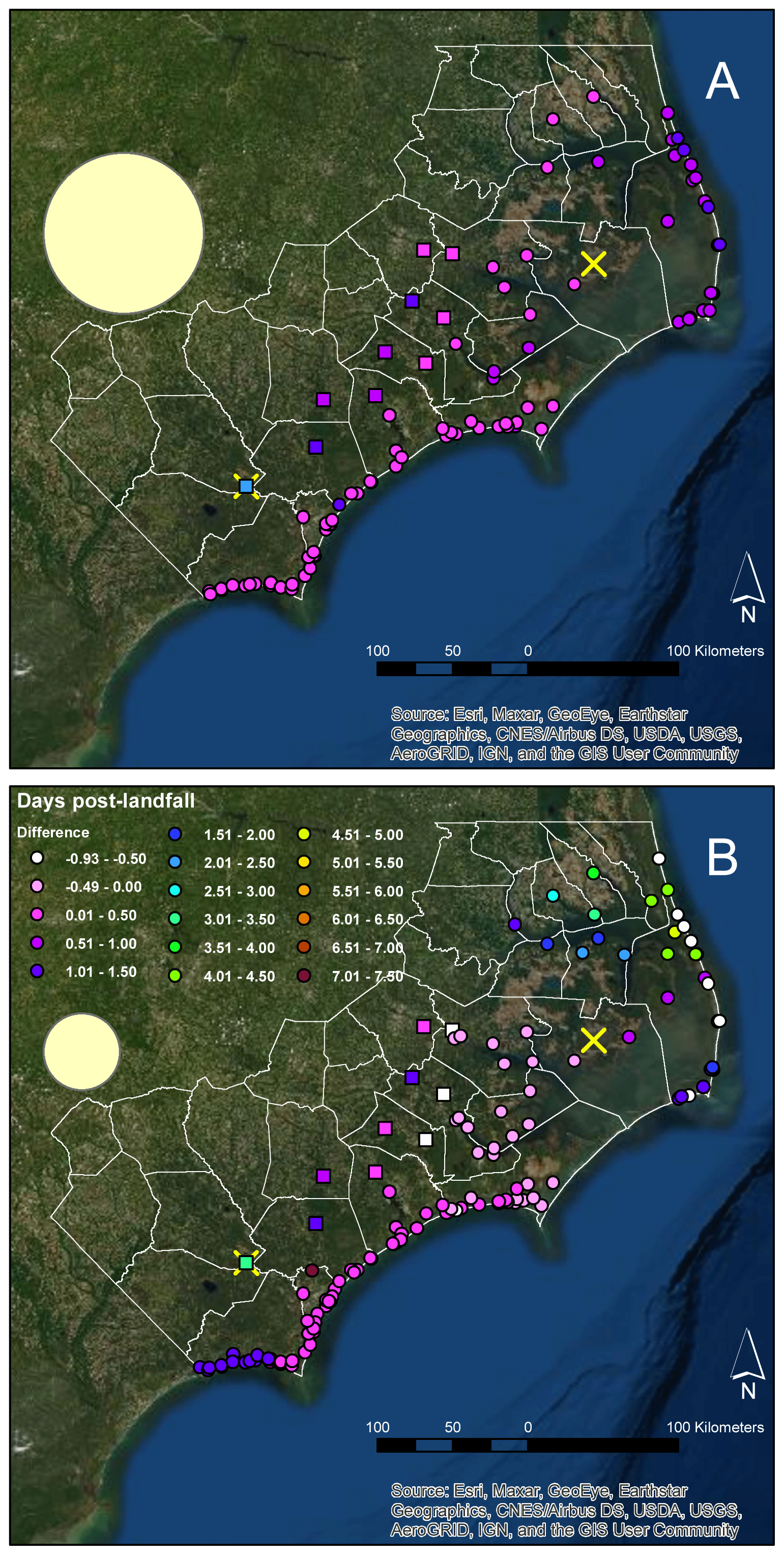
Figure 4Maps of Δtps-lf (circles), time when river gauges first reached minor flood stage (squares), and locations of rain gauges (crosses). Large circles represent the area of similarity in Δtps-lf computed using the semivariogram range (a) as the radius. Panel (a) is for Matthew and (b) is for Florence.
Table 3Moran's I statistic and associated p value for Δtps-lf for hurricanes Matthew and Florence.
Matthew and Florence can both be considered multivariate compound flood events which not only produced surge flooding but also pluvial and fluvial flooding. However, real-time data collection from stream and precipitation gauges during the storms were more limited in the coastal environment: 10 stream gauges (squares in Fig. 4) and 2 rain gauges (X's in Fig. 4) were analyzed to complement the more comprehensive surge analysis. Figure 3b (Fig. 3c) shows 15 min precipitation data during Hurricane Matthew (Florence) and the time when the stream gauges first reached minor flood stage. The timescales were adjusted to match Fig. 3a. Lake Mattamuskeet near Fairfield, NC (northern X in Fig. 4), had higher rainfall totals for Matthew (166.8 mm) compared to Florence (103.1 mm), with a maximum rain rate of 15.2 mm in 15 min (∼61 mm h−1). Heavy rainfall, defined as >2.5 mm in 15 min or >10 mm h−1 (Met Office, 2011) was first observed at the beginning of Matthew's period of record (POR) and last observed 15.25 h after landfall, both at Lake Mattamuskeet. Interestingly, for both storms Cape Fear Lock #1 near Kelly, NC (southern X in Fig. 5), had the highest rainfall totals, recording 204 mm for Matthew and an astounding 622 mm of rainfall during Florence. This hurricane was a massive rainstorm in the southeastern portion of the study area. However, Florence's first instance of heavy rainfall occurred at Lake Mattamuskeet at the beginning of the POR. Lock #1 recorded its first instance of heavy rainfall 4.75 h prior to landfall and its last over 3.5 d after landfall, reaching a peak of 21.3 mm of rain in 15 min (85.3 mm h−1). Most of the stream gauges for both storms reached minor flood stage from landfall to 1.4 d after (Fig. 3b and c). However, for Florence, three streams reached minor flood stage prior to landfall: Swift Creek near Streets Ferry, NC, Trent River near Pollocksville, NC, and Pamlico River at Washington, NC (see squares in Fig. 4b). Also, during Florence Lock #1 (same location as rain gauge) reached flood stage 3.2 d after landfall (Fig. 3c). Thus, the precipitation, stream, and tide data paint a consistent picture that Matthew's flooding across eastern North Carolina was more synchronized as compared to Florence.
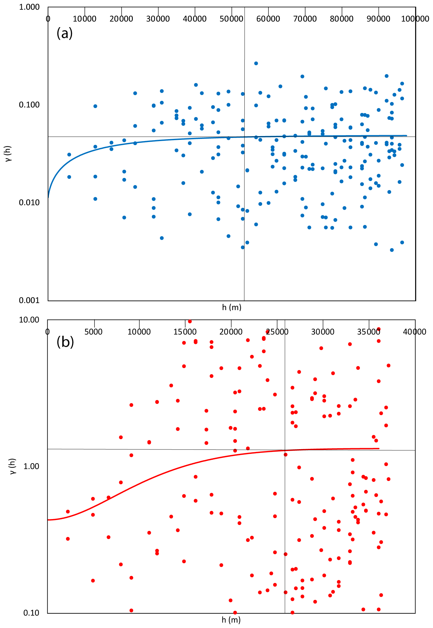
Figure 5Observed values (points) and stable semivariogram models (curves) for γ (h) in the case of (a) Matthew and (b) Florence. X axis is in meters. Y axis is a log-scale. Vertical line denotes the range (a) and horizontal line the sill (Co) (see Table 4).
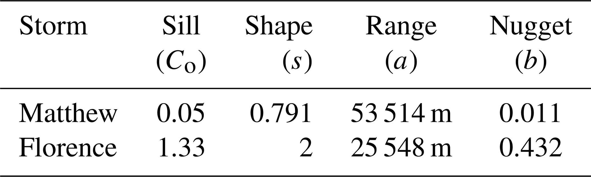
In the final part of the analysis, semivariograms are used to determine a spatial scale of the storm tide hazards for Matthew and Florence. Table 4 gives the parameters of the stable semivariogram functions, and Fig. 5 shows the raw and modeled data. Since the variance of the difference in x(γ) increases with distance, the semivariogram can be considered a dissimilarity function. Florence (Fig. 5b) has much larger values of γ than Matthew (Fig. 5a), even with small distances (notice the difference in scales in Fig. 5). For the stable model, Florence reaches a sill of 1.33 at a range of 25.5 km, while Matthew reaches a sill of 0.05 at a range of 53.5 km (Table 4, Fig. 5). The shape parameter of Matthew is less than 2, which means the stable model resembles an exponential curve more than in the case of Florence. In fact, the exponential model, used by Touma et al. (2018), produced an unphysical range of 1.3 km for Florence (the smallest binned distance is 2.1 km) versus 36.8 km for Matthew. The range is an important quantification of the length scale of timing of peak storm tide. In other words, for the case of Matthew (Florence) one would need to be 53.5 km (25.5 km) distant from a given tide station to reach a dissimilar tide station in terms of Δtps-lf. This range (or radius of similarity) is graphically represented by the yellow circles in Fig. 4. For Matthew the circle (or surge hazard zone) has an area of 8997 km2 and is roughly the size of three eastern North Carolina counties, whereas the Florence surge hazard zone is less than one quarter of the size at 2051 km2.
Table 4Statistics of the stable semivariogram models (see Fig. 6) of Δtps-lf for hurricanes Matthew and Florence.
This study contributes to our understanding of a spatially compounded event or “multiple-connected locations affected by the same or different hazards, within a limited time window, thereby causing an impact” (Zscheischler et al., 2020). In order to account for the “multiple-connected locations” and “limited time window”, the time of hazard is analyzed geospatially within a predetermined region. We apply this definition to storm tide, specifically the peak height recorded, during hurricanes Matthew and Florence for coastal North Carolina. A Moran's I test was used to determine whether there was a clustering of coincident surge hazards, and a semivariogram analysis was used to model the relationship between time of peak surge and distance. The first peak surge during Matthew occurred 15 min prior to landfall, and the last one occurred 28.5 h after landfall. In contrast, the first peak surge during Florence occurred 22.25 h before landfall, and the last one occurred over 7 d after landfall. It is not surprising then that both statistical tests definitively show that Matthew's peak surges happened more simultaneously than Florence. Furthermore, river flooding and extreme rainfall also occurred within a narrower time interval for Matthew as compared to Florence. One important output from the semivariogram analysis is the range or length scale of similarly timed peak surge. For Matthew this “area of effective hazard zone” was 4 times as large as Florence, suggesting that given the same resources, there would be a greater risk of isolation, injury, and death in coastal communities due to surge from Matthew as compared to Florence. However, it should be noted that there were no direct deaths associated with storm surge from either storm. According to the Associated Press (2018) North Carolina Governor Roy Cooper noted that twice as many people were saved from rising floodwaters during Florence as compared to Matthew. This could partially be due to the timing of the water hazards, but more likely it is due to the ever-increasing preparedness for storms by the NCDEM, Swiftwater, and other related agencies.
In summary, this work adds to previous compound hazard studies by applying conventional geospatial analysis techniques to surge within a storm environment. However, there are important caveats to this study that need mention. First, because Matthew was the more spatially compounded storm does not necessarily mean it was the more devastating surge event. In fact, one could argue that because Florence was long lasting and affected different regions of the coast at different times, it was more difficult to manage. At the same time, a more spatially compounded event would make a coordinated response effort and/or reciprocity across counties more challenging. Second, we did not consider the spatial extent of surge flooding, only the tide gauge locations. Schaffer-Smith et al. (2020) found the total flood extent was similar between the two storms in North Carolina, with Florence causing more extensive flooding in the southeastern part of the state. Third, this is a purely statistical study and does not offer reasons for the difference in spatial compounding between Matthew and Florence. However, it is clear that many characteristics of the two storms were quite different as presented in Fig. 2. Unlike Matthew, Florence moved slowly westward so that portions of the coast received onshore winds for an extended period of time covering several tide cycles. After Florence departed the study area and recurved to the north (not shown), it interacted with a high-pressure system over the Atlantic producing southeasterly winds over the estuaries. This may explain why tide gauges in Perquimans, Pasquotank, and Currituck counties had not recorded their highest values until 17 and 18 September. Track, size, translational speed, tides, etc. would all be considered the drivers of this type of spatially compounded hazard, and the storm would be the modulator (Fig. 6). Finally, this study motivates future work to consider a climatology of storm characteristics for developing relationships between the compound hazard drivers and the spatial metrics of surge presented here. Operationally, forecasted storm parameters could then be used in emergency response preparation, with the level of spatial compounding informing the number and distribution of response teams.
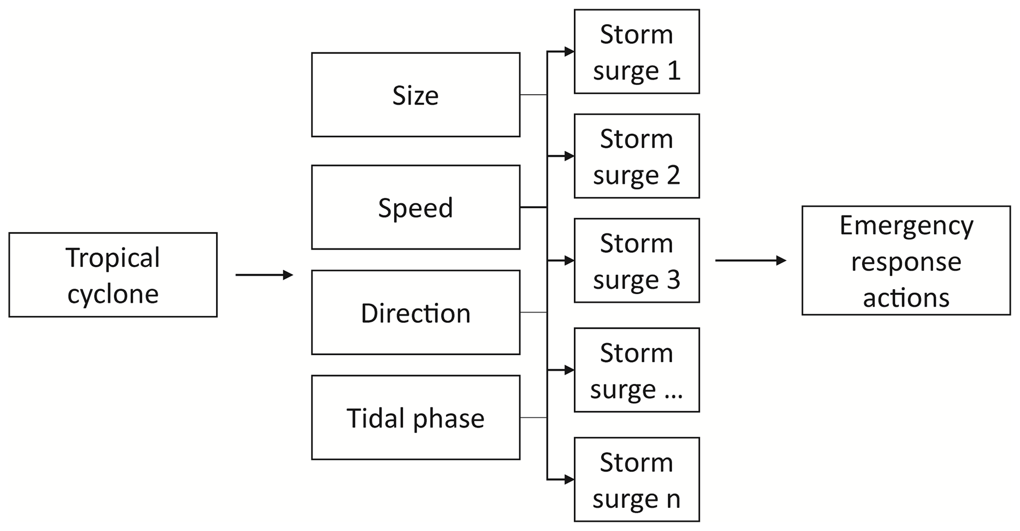
Figure 6Elements that make up a spatially compounded surge hazard, as described in this study (see Zscheischler et al., 2020).
The data used in this paper can be requested from the corresponding author. We ask interested researchers to please contact the corresponding author of this article.
SC collected and analyzed the data, created the tables and figures, and wrote the initial draft. KD, JM, AM, JH, AG, and PVW contributed to the interpretation of the results and reviewed the manuscript.
The authors declare that they have no conflict of interest.
This article is part of the special issue “Understanding compound weather and climate events and related impacts (BG/ESD/HESS/NHESS inter-journal SI)”. It is not associated with a conference.
The authors would like to thank two anonymous reviewers for their important contributions which improved the original manuscript.
This research has been supported by the National Oceanic and Atmospheric Administration (grant no. NA19OAR4310312).
This paper was edited by Ricardo Trigo and reviewed by two anonymous referees.
Associated Press: The latest: Death toll rises to 43 in aftermath of Florence, available at: https://apnews.com/article/92a8fd9b30854c1285ebe019ce8b6851 (last access: 18 December 2020), 21 September 2018.
Blanchet, J. and Creutin, J. D.: Co-occurrence of extreme daily rainfall in the French Mediterranean region, Water. Resor. Res., 54, 2233–2248, https://doi.org/10.1002/2017WR020717, 2017.
Brunner, M. I., Gilleland, E., Wood, A., Swain, D. L., and Clark, M.: Spatial dependence of floods shaped by spatiotemporal variations in meteorological and land-surface processes, Geophys. Res. Lett., 47, e2020GL088000, https://doi.org/10.1029/2020GL088000, 2020.
Du, Y., Xie, Z. Q., and Miao, Q.: Spatial scales of heavy Meiyu precipitation events in eastern China and associated atmospheric processes, Geophys. Res. Lett., 47, e2020GL087086, https://doi.org/10.1029/2020GL087086, 2020.
Koks, E. E., Rozenberg, J., Zorn, C., Tariverdi, M., Vousdoukas, M., Fraser, S. A., Hall, J. W., and Hallegatte, S.: A global multi-hazard risk analysis of road and railway infrastructure assets, Nat. Commun., 10, 2677, https://doi.org/10.1038/s41467-019-10442-3, 2019.
Leonard, M., Westra, S., Phatak, A., Lambert, M., van den Hurk, B., Mcinnes, K., Risbey, J., Schuster, S., Jakob, D., and Stafford-Smith, M.: A compound event framework for understanding extreme impacts, Wiley Interdisciplin. Rev.: Clim. Change, 5, 113–128, https://doi.org/10.1002/wcc.252, 2014.
Met Office: Fact sheet No. 3 – Water in the atmosphere 2011, available at: https://web.archive.org/web/20120114162401/http://www.metoffice.gov.uk/media/pdf/4/1/No._03_-_Water_in_the_Atmosphere.pdf (last access: 18 December 2020), 2011.
Moftakhari, H. R., Salvadori, G., AghaKouchak, A., Sanders, B. F., and Matthew, R. A.: Compound flooding effects of sea level rise and fluvial flooding, P. Natl. Acad. Sci. USA, 114, 9785–9790, https://doi.org/10.1073/pnas.1620325114, 2017.
Munroe, R., Crawford, T., and Curtis, S.: Geospatial analysis of space-time patterning of ENSO forced daily precipitation distributions in the Gulf of Mexico, Prof. Geogr., 66, 91–101, https://doi.org/10.1080/00330124.2013.765291, 2014.
Narayanan, L. and Ibe, O. C.: A joint network for disaster recovery and search and rescue operations, Comput. Netw., 56, 3347–3373, https://doi.org/10.1016/j.comnet.2012.05.012, 2012.
NHC: Storm surge overview, available at: https://www.nhc.noaa.gov/surge/, last access: 18 December 2020.
Rappaport, E. N.: Fatalities in the United States from Atlantic tropical cyclones: New data and interpretation, B. Am. Meteorol. Soc., 95, 341–346, https://doi.org/10.1175/BAMS-D-12-00074.1, 2014.
Raymond, C., Horton, R. M., Zscheischler, J., Martius, O., AghaKouchak, A., Balch, J., Bowen, S. G., Camargo, S. J., Hess, J., Kornhuber, K., Oppenheimer, M., Ruane, A. C., Whal, T., and White, K.: Understanding and managing connected extreme events, Nat. Clim. Change, 10, 611–621, https://doi.org/10.1038/s41558-020-0790-4, 2020.
Schaffer-Smith, D., Myint, S. W., Muenich, R. L., Tong, D., and DeMeester, J. E.: Repeated hurricanes reveal risks and opportunities for social-ecological resilience to flooding and water quality problems, Environ. Sci. Technol., 54, 7194–7204, https://doi.org/10.1021/acs.est.9b07815, 2020.
Stewart, S. S.: Hurricane Matthew, National Hurricane Center Tropical Cyclone Report, National Hurricane Center, Miami, FL, USA, 96 pp., 2017.
Stewart, S. S. and Berg, R.: Hurricane Florence, National Hurricane Center Tropical Cyclone Report, National Hurricane Center, Miami, FL, USA, 98 pp., 2019.
Touma, D., Michalak, A. M., Swain, D. L., and Diffenbaugh, N. S.: Characterizing the spatial scales of extreme daily precipitation in the United States, J. Climate, 31, 8023–8037, https://doi.org/10.1175/JCLI-D-18-0019.1, 2018.
Touma, D., Stevenson, S., Camargo, S. J., Horton, D. E., and Diffenbaugh, N. S.: Variations in the intensity and spatial extent of tropical cyclone precipitation, Geophys. Res. Lett., 46, 13992–14002, https://doi.org/10.1029/2019GL083452, 2019.
Zscheischler, J., Westra, S., van den Hurk, B. J. J. M., Seneviratne, S. I., Ward, P. J., Pitman, A., AghaKouchak, A., Bresch, D. N., Leonard, M., Wahl, T., and Zhang, X.: Future climate risk from compound events, Nat. Clim. Change, 8, 469–477, https://doi.org/10.1038/s41558-018-0156-3, 2018.
Zscheischler, J., Martius, O., Westra, S., Bevacqua, E., Raymond, C., Horton, R. M., van den Hurk, B., AghaKouchak, A., Jézéquel, A., Mahecha, M. D., Maraun, D., Ramos, A. M., Ridder, N. N., Thiery, W., and Vignotto, E.: A typology of compound weather and climate events, Nat. Rev.: Earth Environ., 1, 333–347, https://doi.org/10.1038/s43017-020-0060-z, 2020.