the Creative Commons Attribution 4.0 License.
the Creative Commons Attribution 4.0 License.
 | 21 Apr 2021
Exploring the potential relationship between the occurrence of debris flow and landslides
Zhu Liang
Donghe Ma
Kaleem Ullah Jan Khan
The present study is to explore the potential relationship between debris flow and landslides by establishing susceptibility zoning maps (SZMs) separately with the use of random forest (RF). Lhünzê county, located in southeastern Tibet, was selected as the study area. The work was carried out with the following steps: (1) an inventory map consisting of 399 landslides and 49 debris flows was determined; (2) slope units and 11 conditioning factors were prepared for the susceptibility modeling of landslide while watershed units and 12 factors were prepared for debris flow; (3) SZMs were constructed for landslide and debris flow, respectively, with the use of RF; (4) the performance of two models was evaluated by 5-fold cross-validation using receiver operating characteristic (ROC), area under the curve (AUC) and statistical measures; (5) the potential relationship between landslide and debris flow was explored by the superimposition of two zoning maps; (6) the Gini index was applied to determine the major factors and analyze the difference between debris flow and landslides; (7) a combined susceptibility map with two considered hazardous phenomena was obtained. Two used models had demonstrated great predictive capabilities, with an accuracy of 87.33 % and 85.17 % and AUC of 0.902 and 0.892, respectively. Comparing the overlap of different susceptibility classes for two obtained maps, it was concluded that there is no straightforward relationship between the occurrence of debris flow and landslides. Although most landslides can be converted into debris flow, the area prone to debris flow did not promote the occurrence of a landslide. A susceptibility zoning map composed of two or more hazardous phenomena is comprehensive and significant in this regard, which provides a valuable reference for research studies of disaster-chain and engineering applications.
- Article
(11622 KB) - Full-text XML
- BibTeX
- EndNote


Soil slide and debris flow are two kinds of natural phenomena mainly occurring in mountainous areas, which pose considerable threats to people, industries, and the environment directly or indirectly. Generally, damages can be decreased to a certain extent by predicting the likely location of future disasters (Pradhan, 2010). Thus, extensive research has been conducted for the prediction and susceptibility assessment of landslide and debris flow.
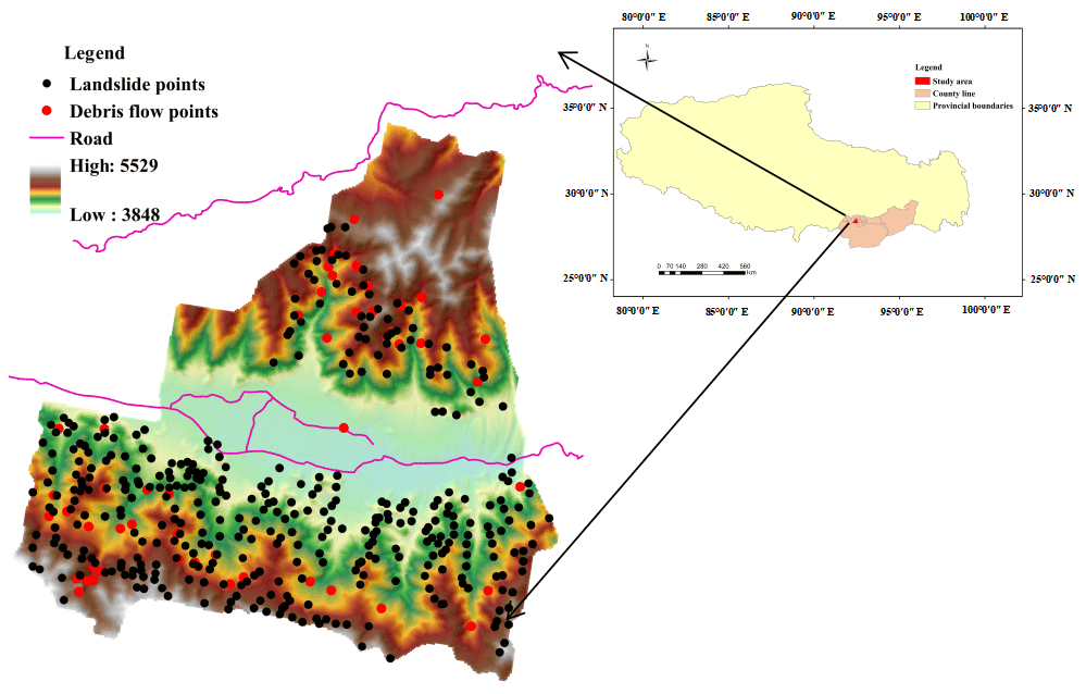
Figure 1Location map of the study area showing the landslide and debris flow inventory.
In geomorphology, a “landslide” is the movement of a mass of rock, debris or earth down a slope under the influence of gravity (Cruden and Varnes, 1996). According to different variables, landslides can be divided into different types (Varnes, 1978). Debris flow is a specific type of landslide, which can be defined as a “Very rapid to extremely rapid surging flow of saturated debris in a steep channel” (Hungr et al., 2013). Most of debris flows are runoff generated (Imaizumi et al., 2006; Theule et al., 2012; Ma et al., 2018). Generally, landslides that occur on a steep slope and become disaggregated as they tumble down can transform into debris flows if they contain sufficient water for saturation (Huang et al., 2019). Debris flow usually occurs on a channel bed for the entrainment into abundant runoff of debris supplied by deep or shallow slides of slopes incised by the channel (Hurlimann et al., 2013; Zhou et al., 2019; Simoni et al., 2020). Therefore, landslides may provide sufficient material source for debris flow, and most of the landslides are accompanied by debris flow (Iverson et al., 1997; Lan et al., 2004). The conditioning factors and mapping units involved in the susceptibility assessment for different kinds of landslides are not identical. In the past, some scholars made separate evaluations between landslide and debris flow. Some scholars have explored the mobilization of debris flow from landslides, and the material source of the debris flow is not necessarily coming from landslides (Chiang et al., 2012; Gomes et al., 2013). Besides, the formation and manifestations of landslides and debris flow are different. In other words, there is no determined connection between debris flow and landslides. However, seldom research studies have explored the potential relationship between debris flow and landslides through the separated susceptibility maps (Alessandro et al., 2015).
The methods used for the susceptibility assessment can be broadly classified as qualitative or quantitative (Aleotti and Chowdhury, 1999). There are different types of quantitative methods: those that are physically based (Carrara et al., 2008), those that are heuristic (Blais-Stevens and Behnia, 2016) and those that are statistically based. Recently, new machine learning models have been used for susceptibility analysis: neural networks (Park et al., 2013), support vector machines (Colkesen et al., 2016) and random forest (RF) (Liang et al., 2020a).
The present study is to explore the potential relationship between the occurrence of debris flow and landslides by establishing susceptibility zoning maps separately with the use of RF. The Lhünzê county in southeastern Tibet is exposed to landslide and debris flow and chosen as the study area.
2.1 Study area
The study area located in Lhünzê township, Lhünzê county, southeastern Tibet, is bounded by longitudes of 92∘15′ and 92∘45′ E and latitudes of 28∘10′ and 28∘30′ N (Fig. 1). It covers a surface of about 535 km2 with a population of more than 6000. It belongs to a semi-arid temperate monsoon climate with the annual rainfall of 279 mm, mainly concentrated in May to September. The seismic intensity within the area has a degree of VIII on the modified Mercalli index.
The study area is distributed in the zone of stratigraphic division of the Northern Himalayan block. The strata are mainly composed of Mesozoic Cretaceous, Jurassic, Triassic and Cenozoic units. Three types of lithology were mainly observed during our field investigation: siltstone from the Laka Formation (), conglomerates from the Weimei Formation () and Quaternary slope wash () from the Cenozoic strata.
Main disasters in the study area consist of rain-fed high-frequency debris flows and landslides, which destroyed and flooded roads, bridges, farmland, villages, etc., causing great economic losses.
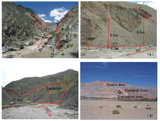
Figure 2Photos of landslide or debris flow: (a) Lunba landslide in a tributary, (b) Zhenqiong landslide in Jiayu village, (c) debris flow in Misha township and (d) debris flow in Lelong village.
2.2 Landslide and debris flow inventory
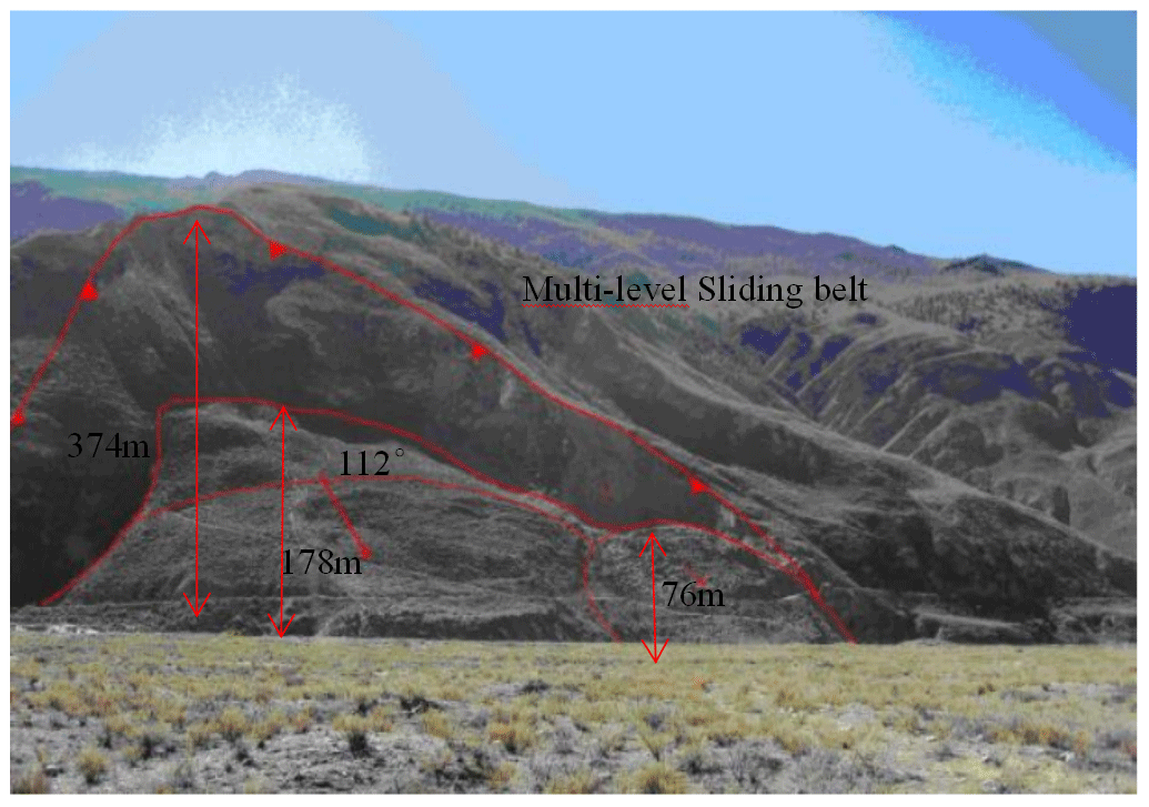
The statistically based susceptibility models are based on an important assumption: future landslides have more chances to occur again under the conditions which led to the past and present landslides (Varnes, 1984). Therefore, a complete inventory map is the key for modeling. In this study, data come from historical records (1970–2010), field surveys from 200–2003 (Figs. 2 and 3) and interpretation of Google Earth images carried out in Google Earth Pro 7.1 (Fig. 4). Finally, a total of 399 landslides and 49 debris flow locations with positive label were recorded and mapped as a point (Fig. 1), and the same number of non-landslide points with a negative label were selected randomly from the landslide-free area.
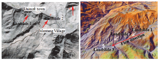
Figure 4Remote sensing map of landslides in Lhünzê township (Tong et al., 2019): (a) landslides in Lhünzê town and (b) landslides in Malu town.
2.3 Mapping units
The selection of the mapping unit is an important prerequisite for modeling (Guzzetti et al., 2006a). The mapping units commonly used are grid cells (Reichenbach et al., 2018). Despite their popularity and operational advantages, grid cells have clear drawbacks (Guzzetti et al., 1999). There is no physical relationship between a grid cell or a group of grid cells and slope, while slope units can make up for this deficiency. A slope unit may correspond to an individual slope, an ensemble of adjacent slopes or a small catchment. The geometry of the debris flow is tortuous and complex, which is not not suitable to be represented with a regular grid unit. In the present study, adjacent slope units were applied to the modeling. First-order subcatchments, which are also called watershed units, were applied to the susceptibility of debris flow (Bregoli et al., 2015; Liang et al., 2020b). Accordingly, the study area was divided into 1003 slope units for the modeling of landslides or 174 watershed units for debris flow.
2.4 Controlling factors and mapping
The selection of evaluation parameters is another key prerequisite to ensure that the model is accurate. Different research studies emphasized different controlling factors, but the availability, reliability and practicality of the data were first considered (van Westen et al., 2008). In this paper, 11 controlling factors are selected for landslide susceptibility assessment and 12 for debris flow. A brief description of each controlling factor is given below. Detailed information is shown in Fig. 5a–m.
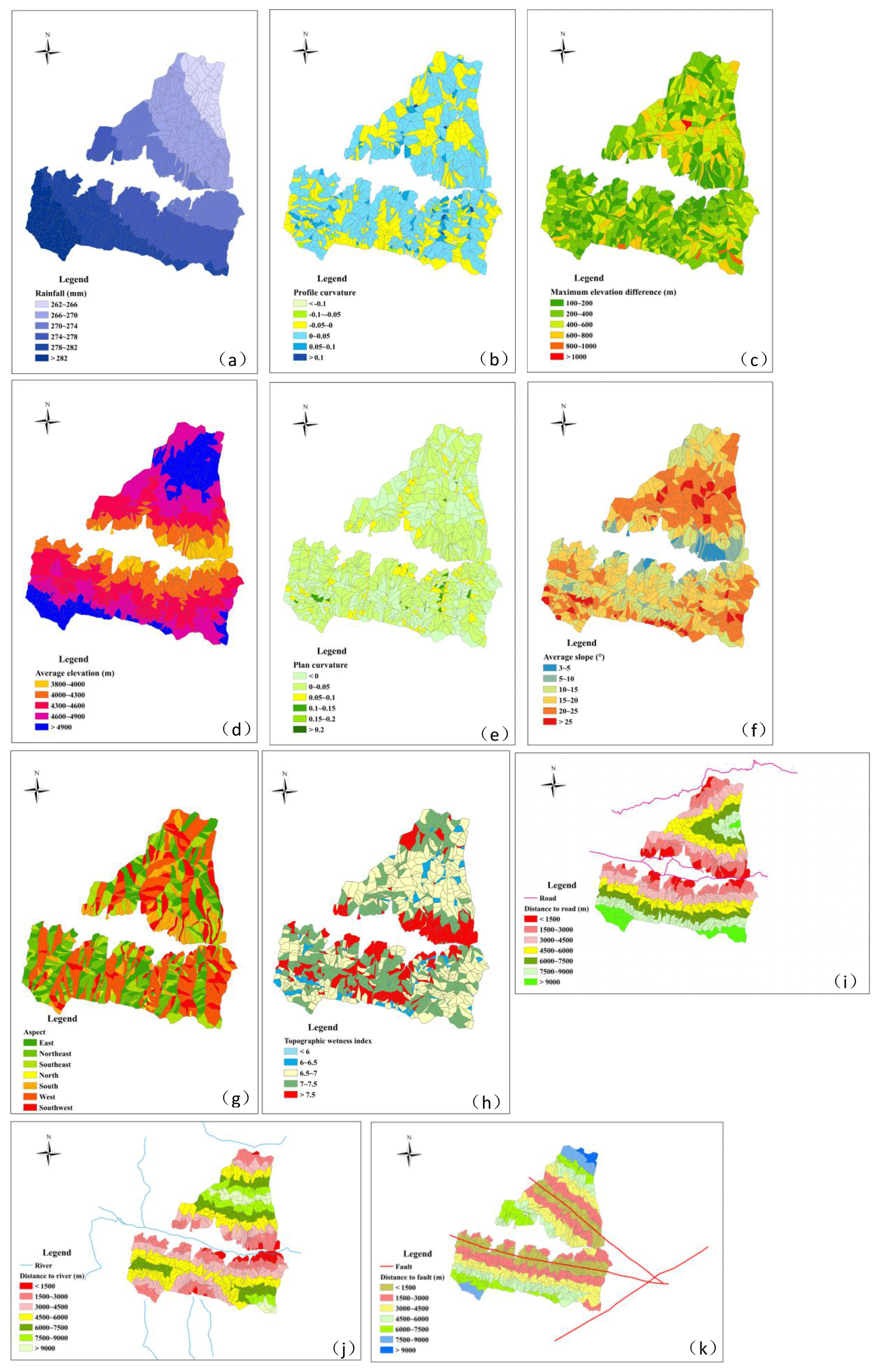
Figure 5Study area thematic maps for landslide: (a) rainfall, (b) profile curvature, (c) maximum elevation difference, (d) average elevation, (e) plan curvature, (f) average slope, (g) aspect, (h) wetness, (i) distance to road, (j) distance to river and (k) distance to fault.
2.4.1 Factors used in landslide susceptibility assessment
The aspect reflects sunshine duration and rainfall, which is frequently used as a landslide controlling factor (Dai and Lee, 2002) and was reclassified into eight classes (Fig. 5g). Plan curvature and profile curvature, which reflect the relief of the terrain, were both considered and reclassified into six classes (Fig. 5b and e). Generally, faults, rivers and roads play a key role in the occurrence of landslides as landslides are more likely disturbed around faults, rivers and roads (Taskin et al., 2015), which were reclassified into seven classes using an interval of 1500 m (Fig. 5i–k). The topographic wetness index (TWI) belongs to a hydrological variable that reflects both slope and soil moisture content (Wilson and Gallant, 2000) and was reclassified into five classes (Fig. 5h).
2.4.2 Factors used in debris flow susceptibility assessment
The pre-event normalized difference vegetation index (NDVI) reflects the vegetation conditions in the area and was reclassified into five classes (Fig. 6b). The drainage density is the ratio of the total drainage length to the watershed area and was reclassified into six classes (Fig. 6g). The roundness refers to the ratio of the area of a basin to the area of a circle with the same circumference and was reclassified into six classes (Fig. 6d). The Melton ratio refers to the ratio of the degree of undulation in the watershed to the square root of the arithmetic area of the watershed (Melton, 1965), which is reclassified into seven classes (Fig. 6a). The basin area and main channel length are represented by the same graph and were reclassified into four classes (Fig. 6h). The average gradient of main channel, which is the ratio of the maximum elevation difference of main channel to its linear length, was reclassified into six classes (Fig. 6j).
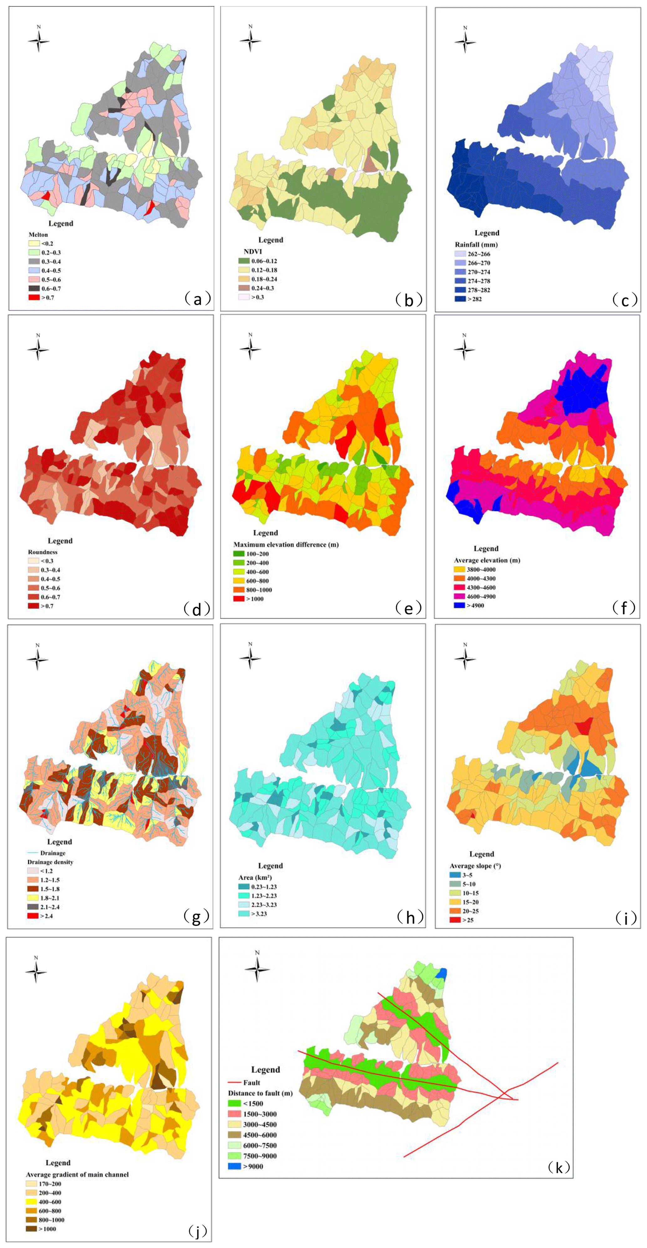
Figure 6Study area thematic maps for debris flow: (a) Melton, (b) NDVI, (c) rainfall, (d) roundness, (e) maximum elevation difference, (f) average elevation, (g) drainage density, (h) area, (i) average slope, (j) average gradient of main channel and (k) distance to fault.
2.4.3 Factors used in both landslide and debris flow
Rainfall is the only triggering factor to be considered for both landslide and debris flow in this paper, which was reclassified into six classes (Figs. 5a and 6c). The slope angle, which reflects kinetic energy conditions, is frequently employed in both landslide and debris flow susceptibility mapping and was reclassified into six classes (Figs. 5f and 6i). The maximum elevation difference also reflects the kinetic energy condition and is reclassified into six classes using an interval of 200 m (Figs. 5c and 6e). Elevation affects the rainfall and vegetation (Figs. 5d and 6f) and was reclassified into five classes in the study (Pourghasemi et al., 2013).
The values of the controlling factors were classified by processing the raw data in the ArcGIS 10.2 platform. Morphological and topographically related factors were derived from the DEM with a resolution of 30×30 m (http://www.gscloud.cn, last access: 5 May 2018). Geologically related factors were extracted from 1:50 000 geological maps (http://www.ngac.org.cn/, last access: 5 May 2018). Rainfall is one of the most important external factors inducing landslides and debris flow, which was determined by ordinary kriging interpolation in ArcGIS based on data from 11 precipitation stations near the study area collected from the China Meteorological Administration. Road networks are provided by Landsat 8 Operational Land Imager (OLI) images (12 August 2018).
3.1 Sampling strategy and performance assessment
Statistical models for landslide susceptibility zoning reconstruct the relationships between dependent and independent variables using the training dataset and verify these relationships using validation sets (Guzzetti et al., 2006b), which usually implies the partitioning of the inventory in subsets. The sampling strategy affects the results of the susceptibility map (Yilmaz, 2010). The partition of the landslide inventory is approached based on temporal, spatial or random criteria (Chung and Fabbri, 2003), and among these the one of random time selection is the most used. However, there is a need for a more reliable estimation of the model performance. The ability of the models to classify independent test data was elaborated using a 5-fold cross-validation procedure (James et al., 2013).
The value of the area under the curve (AUC) is the most popular metric to estimate the quality of model, which has been applied for receiver operating characteristic (ROC) curves (Green and Swets, 1966). Three extra statistical metrics as accuracy, sensitivity and specificity are combined to assess the performance of models.
where TP represents true positives, i.e., cells predicted unstable and observed unstable; TN represents true negatives, i.e., cells predicted stable and observed stable; FP represents false positives, i.e., cells predicted unstable but observed stable; and FN represents false negatives, i.e., cells predicted stable but observed unstable.
3.2 Random forests
RF is a powerful ensemble-learning method and was first introduced by Breiman (2001). The bagging technique is applied to select random samples of variables and observations as the training dataset at each node of the tree for the modeling of RF. Unselected cases (out of bag) are used to calculate the error of the model (OOB error). The increase in OOB error is proportional to the importance of the predictive variable. There are no restrictions on the types of variables, either numerical or categorical. RF has the ability to reduce errors caused by unbalanced data, which are suitable for susceptibility assessment.
The number of trees and the number of predictive variables used to split the nodes are two user-defined parameters (Ahmed et al., 2016). Cross-validation was applied to optimized the hyper-parameters before application. The scikit-learn package (Pedregosa et al., 2011) in the programming software Python version 3.7 was used for the modeling. The Gini index (the larger the value of the obtained result, the greater the contribution to the occurrence of landslide) was applied to analyze the relative importance of conditioning factors.
4.1 Landslide susceptibility mapping results
The predictive accuracy, ROC curves and AUC values of the RF models using the training dataset were shown in Table 1 and Fig. 7. The RF model ensured a satisfactory performance for classifying landslides with a sensitivity value of 91.62 %. In terms of the classification of non-landslide zones, the specificity value also reached 89.06 %. An AUC value ranges from 0.5 to 1, with a value equal to 1 indicating a perfect prediction accuracy (Vorpahl et al., 2012). The RF model had great performance in terms of AUC, with a value of 0.976. Standard error (SE), confidence interval (CI) at 95 % and significance (Sig.) were applied as three evaluation statistics. All these results indicated that the models achieved a reasonable goodness of fit, for which the values were reasonably small.
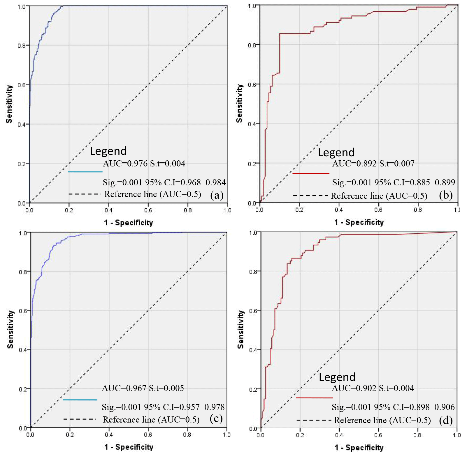
Figure 7Analysis of the ROC curve for the two susceptibility maps: (a) success rate curve of landslide using the training dataset, (b) prediction rate curve of landslide using the validation dataset, (c) success rate curve of debris flow using the training dataset, and (d) prediction rate curve of debris flow using the validation dataset.

Verifying the generalization ability of the model is a key step in prediction models as shown in Table 2 and Fig. 7. Accordingly, the values of sensitivity and specificity were 88.69 % and 86.05 %, respectively. The model also achieved a great performance in terms of AUC with a value of 0.902. In comparison with the training dataset, the accuracy and AUC values have slightly decreased but still perform well.

The landslide susceptibility map was reclassified into five classes – very low (0–0.2), low (0.2–0.4), moderate (0.4–0.6), high (0.6–0.8) and very high (0.8–1) – by using the equal spacing method (Fig. 8). The map should satisfy two spatial effective rules: (1) the existing disaster points should belong to the high-susceptibility class and (2) the high-susceptibility class should cover only small areas (Bui et al., 2012). The number of units belonging to the very high class accounted for 17 % of the total number of units (Fig. 9). Disaster points were mostly in the dark (red or orange) areas. The units belonging to the moderate class accounted for the smallest proportion, at 13 % of the total number of units (Fig. 9).
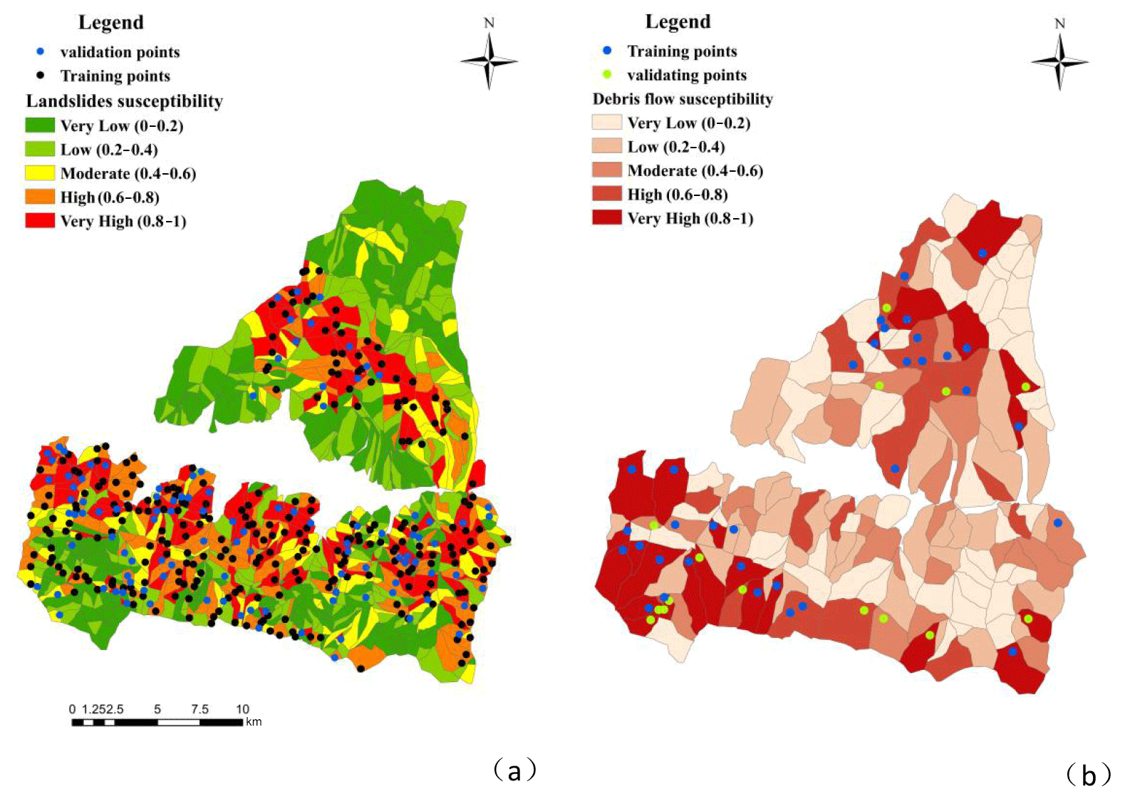
Figure 8Susceptibility maps: (a) landslide susceptibility zoning map and (b) debris flow susceptibility zoning map.

Figure 9Numbers and percentage of units in different susceptibility classes for landslide and debris flow: (a) number of units in different susceptibility classes for landslide and debris flow and (b) percentages of different susceptibility classes for landslide and debris flow.
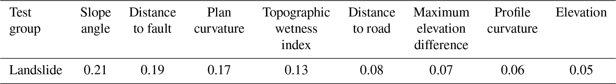
The controlling factors with significant effects were selected and normalized as shown in Table 3. The weight values of slope angle, distance to fault, plan curvature and topographic wetness index were 0.21, 0.19, 0.17 and 0.13, respectively, which was closely related to the occurrence of landslide. The weight values of distance to road, maximum elevation difference, profile curvature and elevation are less than 0.1 as 0.08, 0.08, 0.06 and 0.05, respectively (Fig. 10).
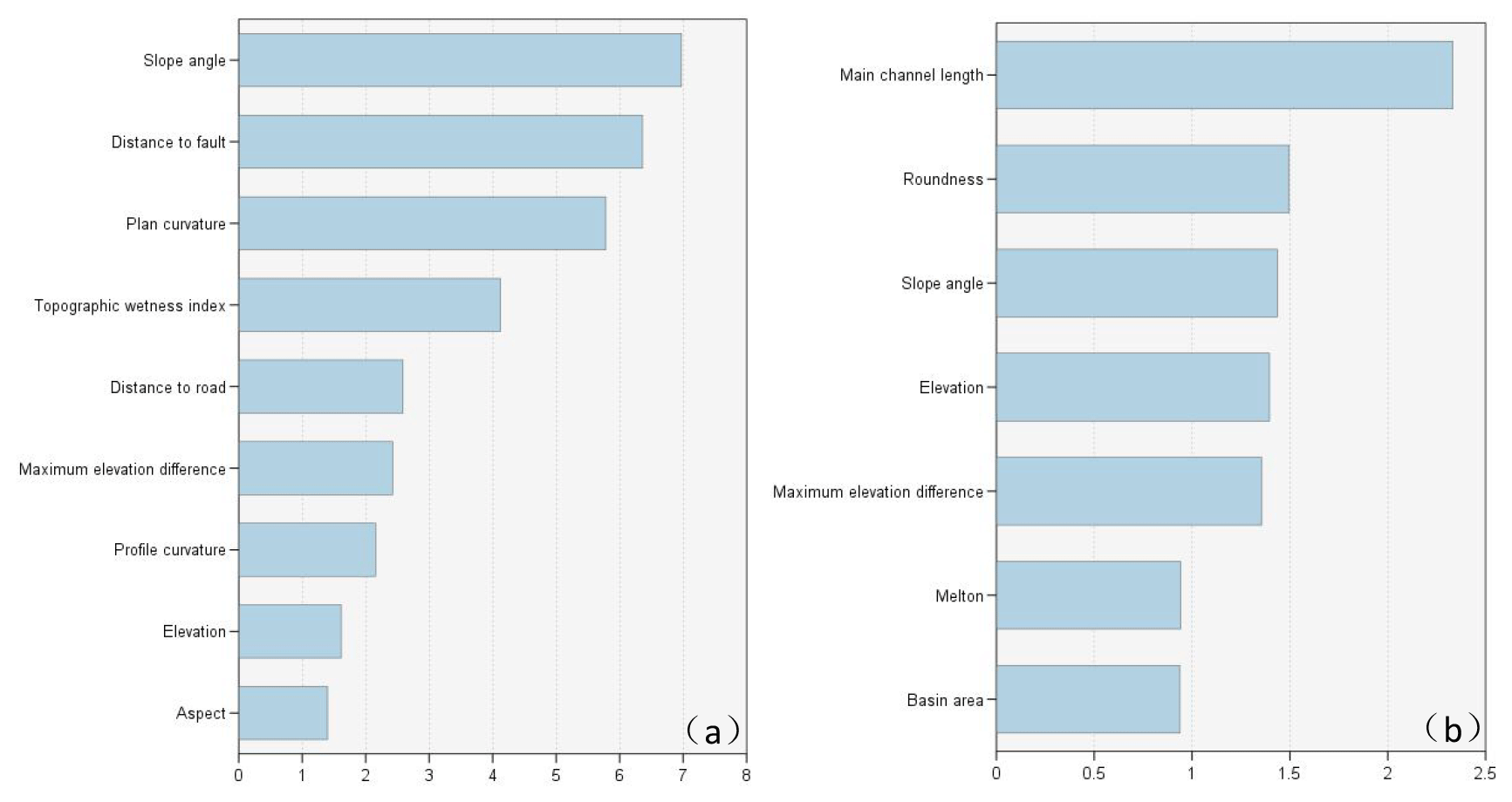
Figure 10Parametric importance graphics obtained from the RF model: (a) parametric importance graphics of landslide and (b) parametric importance graphics of debris flow.
4.2 Debris flow susceptibility mapping result
The debris flow susceptibility model performs well with a very high sensitivity and specificity values of 87.80 % and 88.89 %, respectively. In terms of accuracy and AUC, the model also had a great prediction performance with a value of 88.57 % and 0.967 (Fig. 7). Three evaluation statistics also indicate a reasonable goodness of fit for the model.
Table 2 shows that the values of sensitivity and specificity were 85.71 % and 84.62 %, which were slightly decreased compared to the training model. However, the model had achieved a great performance in terms of AUC, with value of 0.892.
The number of units belonging to the very high class accounted for 15 % of the total number of units, while the units belonging to the high class accounted for the smallest proportion at 13 %. More than half of the units (58 %) belong to on a low or very low class (Fig. 9). Disaster points were mostly in the dark (bright or deep red) areas (Fig. 8).
The weight values of main channel length, roundness and slope angle were 0.25, 0.16 and 0.14, respectively, and these factors have significant influence on the occurrence of debris flow (Table 4). The weight values of elevation, maximum elevation difference, Melton ratio and basin area are close to 0.1, which are 0.13, 0.12, 0.1 and 0.1, respectively (Fig. 10).

4.3 Analysis and comparison of landslide and debris flow susceptibility
It is worth comparing the two susceptibility zoning maps. In terms of prediction accuracy, the values of sensitivity, specificity and AUC of landslide model were slightly higher than that of debris flow. However, both models achieved high predictive performance. Therefore, the landslide and debris flow susceptibility assessment models based on RF are reliable. The purpose of the present study is to explore the potential relationship between landslides and debris flows by establishing the respective susceptibility zoning maps. Figure 11 shows the overlapping areas between debris flow and landslides in a high or very high class of susceptibility zoning maps. It can be seen that most of the areas with a high or very high class in the map of debris flow are covered with landslides. However, there are also non-overlapping areas between the two zoning maps. There are 23 watershed units belonging to the high class in the debris flow susceptibility zoning map (Fig. 8), of which 17 units correspond to the high- or very-high-class slope units in the landslide zoning map (Table 5). In addition, there are 4 watershed units covered with low- or very-low-class slope units. In the same way, 19 watershed units belonging to the very high class are covered with high- or very-high-class slope units and 4 watershed units with low- or very-low-class slope units. In other words, more than 70 % of the high- or very-high-class watershed units are covered with high- or very-high-class slope units. However, there are still 30 % of watershed units with a high or very high class without the distribution of slope units in corresponding grades. This validated the previous view that most of landslides can be transformed into debris flows.
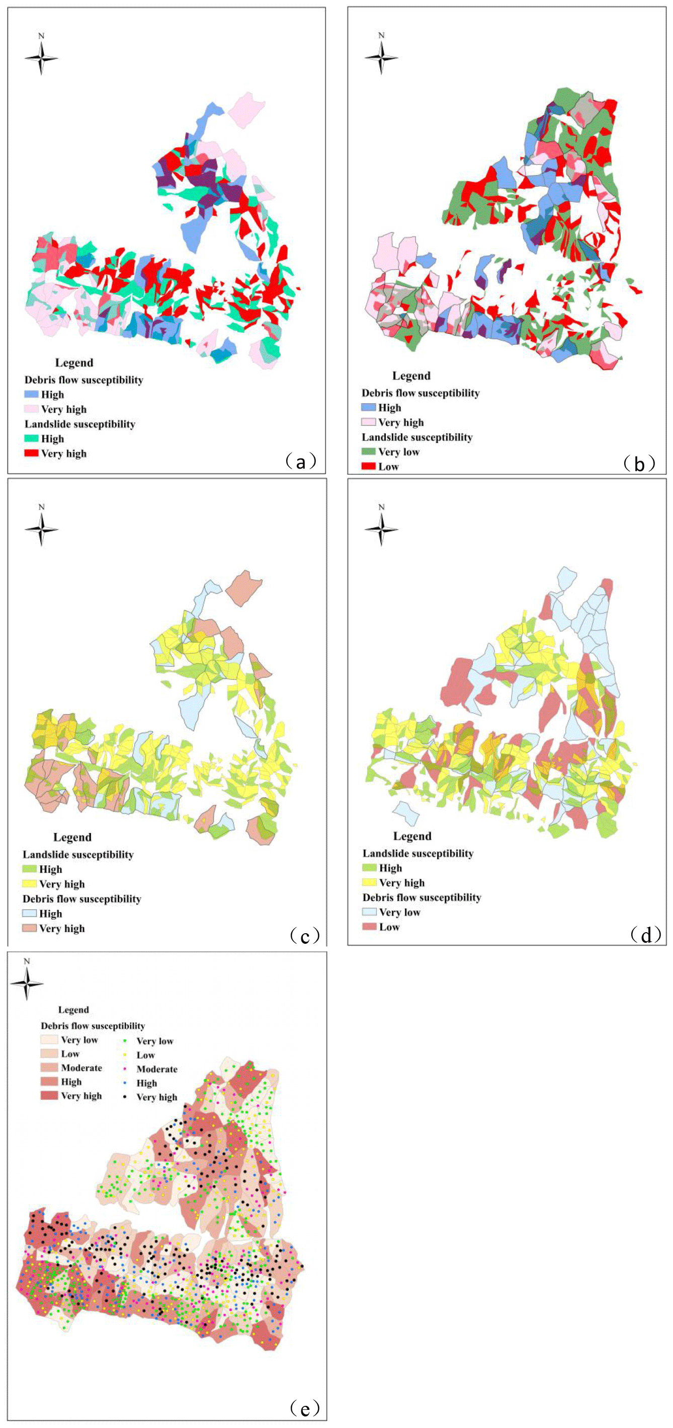
Figure 11Landslide–debris-flow susceptibility maps: (a) high- and very-high-class watershed units with high- or very-high-class slope units, (b) high- or very-high-class watershed units with low- or very-low-slope units, (c) high- or very-high-class slope units with high- or very-high-class watershed units, and (d) mapping units.
Table 5The overlap of the number of debris flow and landslide high- and very-high-class mapping units.

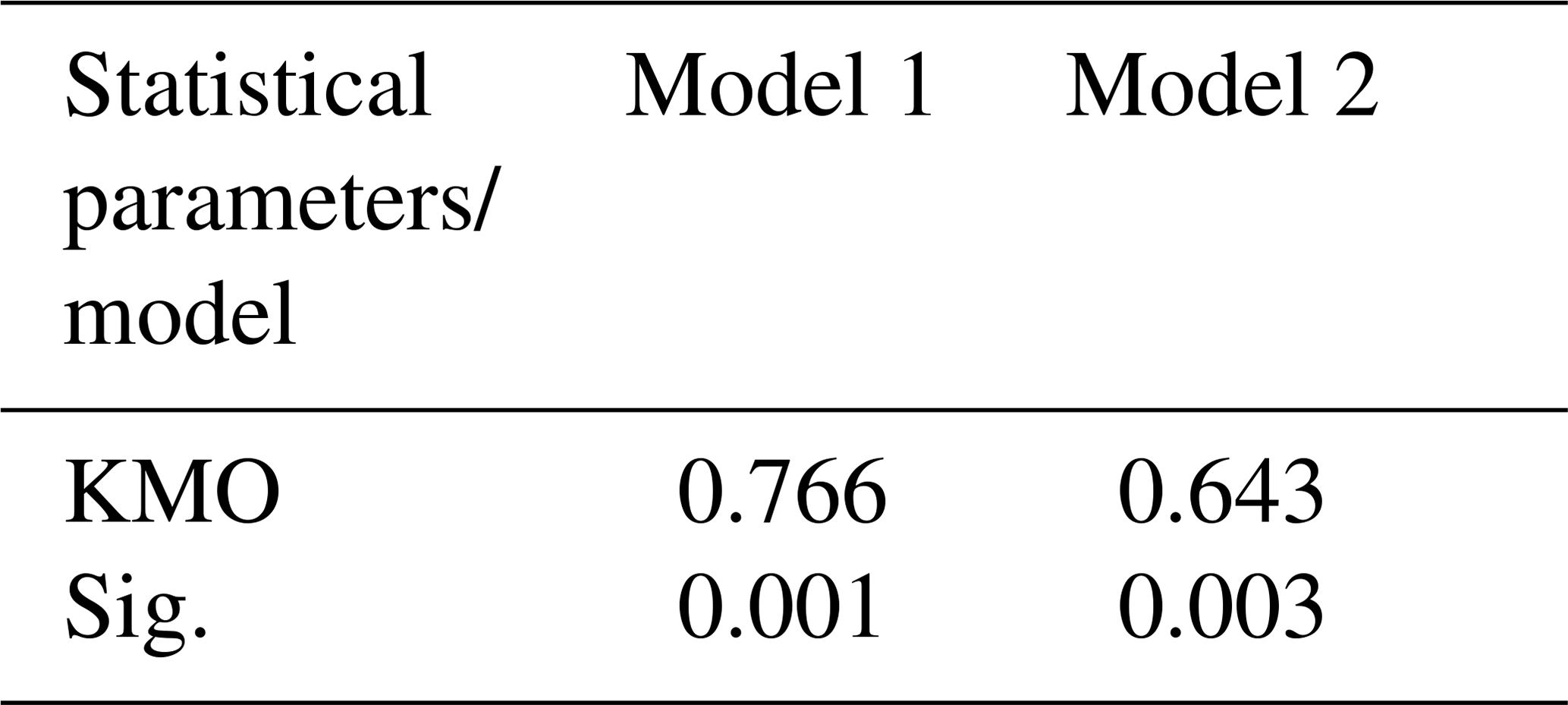
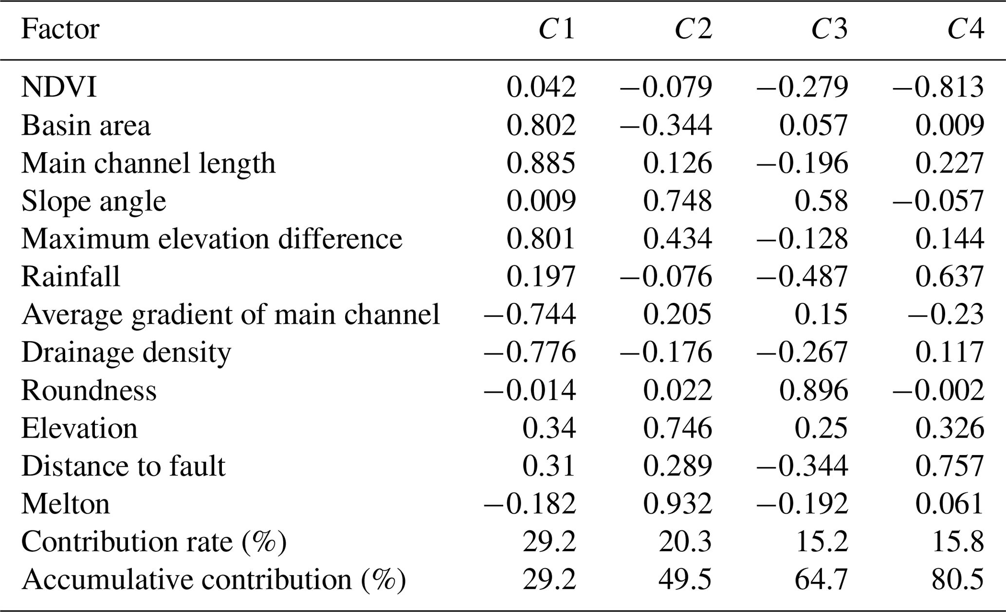
Factor analysis, which is a tool for dimensionality reduction and exploring the major factors, was applied to further analyze the reasons for the difference. Thirty-six watershed units with distribution of high- or very-high-grade slope units were taken as model 1, and the remaining eight watershed units as model 2. The KMO (Kaiser–Meyer–Olkin) and Sig. testing are two statistical parameters which ensured the feasibility before application and are provided by SPSS (Statistical Product and Service Solutions). The closer the KMO statistic is to 1, the stronger the correlation between variables and the better the effect of factor analysis are. The KMO values were 0.766 and 0.643, respectively, which indicated that the correlation between variables was obvious and suitable for factor analysis (Table 6). In model 1, the cumulative contribution rate of the first three factors (C1–C3) reached to 83.6 %, while the cumulative contribution rate of the first four factors (F1–F4) reached to 80.5 % for model 2 (Table 7). According to the correlation coefficient of each common factor, the first common factor mainly highlighted the information of the basin area, main channel length and maximum elevation difference. Similarly, the second and the third common factor highlighted the information of slope angle and elevation and roundness, respectively. The difference between the two models (model 1 and model 2) is that the second model has the fourth common factor (Table 8), which emphasized the effects of rainfall and distance to the fault. The transformation from a landslide to a debris flow often occurs during heavy rainfall (Takahashi, 1978), and the landslides are the source area. But landslides are not the only source of debris flows. The loose material distributed in the basin is not necessarily caused by a landslide.
Table 7The correlation coefficients between common factors and primitive variables.
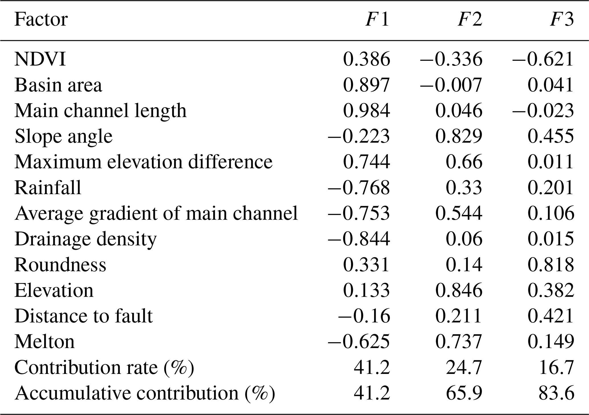
Table 8The correlation coefficients between common factors and primitive variables.
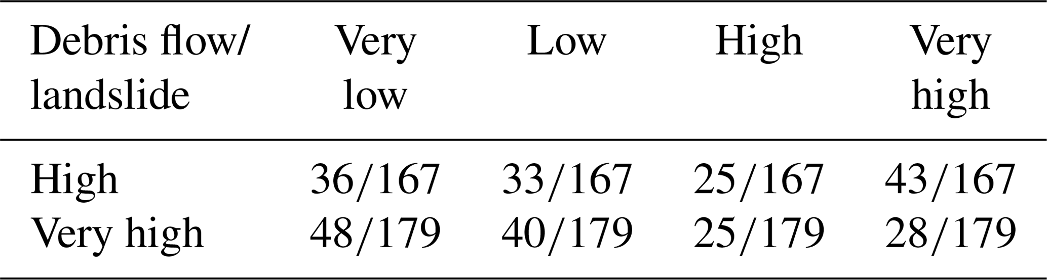
In turn, we analyze the distribution of high- or very-high-class slope units in watershed units. The landslide zoning map was put at the bottom floor and the debris flow zoning map on the top floor (Fig. 11). There are 167 slope units belonging to the high class, of which 68 units (accounting for about 40 %) are distributed in the area of high- or very-high-class watershed units in the debris flow zoning map (Table 9). Besides, 69 slope units (accounting for about 41 %) are distributed in the area of low- or very-low-class watershed units. Similarly, 53 slope units (accounting for about 30 %) belonging to the very high class are distributed in the area of high- or very-high-class watershed units and 88 slope units (accounting for about 50 %) in low- or very-low-class slope units (Table 9). Comparing with the extent of the landslide affecting the debris flow, the impact of the debris flow on the landslide is not obvious. It indicated that the area prone to debris flow does not promote the occurrence of landslides.
Table 9The overlap of the number of landslide and debris flow high- and very-high-class mapping units.
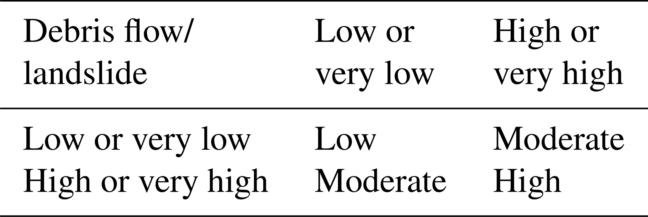
Finally, we took the center of gravity of 1003 slope units as the potential hazard points and spread them over 174 watershed units. Thus, a combining susceptibility zonation map for landslide and debris flow was obtained (Fig. 11). The darker the color, the higher the class of susceptibility will be. It can be seen that the susceptibility in the south is generally higher than that in the north, and the area in the southwest is disaster-prone. The northeast and central locations in the area are less likely to be affected by landslides and belong to low-susceptibility areas. Green or yellow dots, which refer to slope units with very low or low class in the landslide zoning map, are mainly distributed in light-colored areas, but there are also quite a few green or yellow dots distributed in dark areas, which means that the occurrence of debris flow does not necessarily depend on landslides. Blue or black spots are mainly distributed in dark areas, but there are also quite a few blue or black spots distributed in dark areas, which means that a landslide is not the only condition for debris flow to occur. Most of the watershed units are distributed with two or more colored dots, which means that there would be multiple slope units with a different susceptibility class in the same watershed. According to the combining susceptibility zoning map of landslide and debris flow, the study area can be divided into four categories: (1) low- or very-low-class watershed units coupled with low- or very-low-class slope units, (2) low- or very-low-class watershed units coupled with high- or very-high-class slope units, (3) high- or very-high-class watershed units coupled with low- or very-low-class slope units, and (4) high- or very-high-class watershed units coupled with high- or very-high-class slope units. We assume that the occurrence of landslides can bring rich sources of debris flow, thereby promoting or aggravating the outbreak of debris flow, that is, forming a landslide–debris-flow disaster chain. Therefore, the susceptibility assessment of the landslide–debris-flow chain in the study area can be roughly divided into three classes, which are low, moderate and high (Table 10).
Table 10Comprehensive evaluation of landslide–debris-flow susceptibility.
5.1 Method used for modeling
Many researchers have used different statistically based methods to evaluate the susceptibility of landslides or debris flows. Logistic regression and discriminant analysis are the most popular methods to use in traditional multivariate statistical analysis (Teigila, 2015; Abdelaziz et al., 2020). The performance of new learning machines, such as support vector machines and neural networks, has also been verified. RF has been little used until now for susceptibility analysis of landslide and debris flows (Chen et al., 2017; Zhang et al., 2017). Actually, RF has powerful data processing capabilities and can simultaneously solve problems such as high-dimensional, unbalanced and data loss problems, which are common in geological disaster assessment. Most importantly, RF can compare the important differences between features and have ability to reduce errors caused by unbalanced data and which achieved strong generalization properties (Liang et al., 2020a, c).
5.2 Potential relationship between landslide and debris flow
There is a certain similarity in the evaluation of the susceptibility of landslide and debris flow as the selection of controlling factors and the application of modeling strategies. Therefore, some researchers have neglected the difference between landslide and debris flow, i.e., to express two different disasters with the same susceptibility zoning map (Mariantonietta et al., 2017; Maria et al., 2017). However, similarity does not always mean consistency. Many researchers have previously conducted studies into the debris flow mobilization from shallow landslides using a coupled methodology (Lin et al., 2017). However, not every landslide evolves into a debris flow, which means that the analysis process is highly selective or uncertain. In the same way, the source of the debris flow is not limited to landslides. There, the potential relationship between landslide and debris flow needs to be discussed more reasonably and effectively. In this study, the corresponding influencing factors and mapping units are selected to establish landslide and debris flow susceptibility zoning maps, respectively. The potential relationship between landslide and debris flow is explored in two ways: (1) superimposing the high- or very-high-class susceptibility areas in the two maps and (2) transforming the slope units into points and distributing them on the watershed units. The relationship between landslide and debris flow is illustrated by the distribution of slope units of different grades on the watershed units with different susceptibility classes. Different kinds of landslides should be evaluated respectively because of conditioning factors and scale.
5.3 Necessity and feasibility of combining multiple natural disaster susceptibility zoning maps
Previous studies on susceptibility zoning mapping of disasters have agreed that one disaster corresponds to one map. However, it will cause some confusion in practice. For example, multiple disasters may be bred simultaneously in a watershed unit. For another case, the probability of one kind of disaster like debris flow in a watershed is negligible, while another disaster like rockfall occurs frequently. Therefore, we need to combine multiple zoning maps at the same time to give a comprehensive evaluation, which is difficult to achieve. On the one hand, the prediction accuracy and error of different zoning maps should be similar or even consistent. On the other hand, the dimensions of the mapping unit should be consistent or complementary. The fact that the appropriate prediction method (like RF applied in this study) and mapping units were applied to the two disasters makes it possible to merge the two zoning maps. Disaster risk is higher in a landslide–debris-flow chain, causing significant loss of life and property. Therefore, two natural disasters with a potential relationship are simultaneously reflected in the same susceptibility zoning map, which can better guide the implementation of engineering, such as a landslide–debris-flow disaster chain.
In this study, susceptibility assessment models for landslide and debris flow are established through RF, and the performance of the models is excellent in terms of accuracy and goodness of fit. The potential relationship between landslide and debris flow is discussed by the superimposition of two zoning maps, and the following conclusions can be drawn.
-
The landslide and debris flow susceptibility mapping based on RF models have great accuracy and goodness of fit and have the ability to analyze the relative importance of different impact factors, which is suitable for the evaluation of natural disasters.
-
There is no straightforward relationship between the occurrence of the two considered phenomena. Although most landslides will be converted into debris flow, the landslides are not necessarily the source of debris flow, and the loose sources carried by the debris flow are not necessarily brought by the landslides. On the other hand, the impact of the debris flow on the landslide is also not obvious.
-
A susceptibility zoning map composed of two or more natural disasters is more comprehensive and significant, which provides a valuable reference for researchers and engineering applications.
The data used to support the findings of this study are available at https://github.com/Liangzhu-mz/data (last access: 19 April 2021) (Zhu, 2021).
ZL was responsible for the writing and graphic production of the paper. CMW was responsible for the revision of the paper. DHM was responsible for calculation. KUJK was responsible for the translation.
The authors declare that they have no conflict of interest.
This article is part of the special issue “Resilience to risks in built environments”. It is not associated with a conference.
This work was supported by the Graduate Innovation Fund of Jilin University and the National Natural Science Foundation of China (grant nos. 41972267, 41977221 and 41572257).
This research has been supported by the National Natural Science Foundation of China (grant nos. 41972267, 41977221 and 41572257).
This paper was edited by Damien Serre and reviewed by two anonymous referees.
Abdelaziz, M., Ali, P. Y., Jie, D., Jim, W., Binh, T., Dieu, T. B., Ram, A., and Boumezbeur, A. : Machine learning methods for landslide susceptibility studies: A comparative overview of algorithm performance, Earth-Sci. Rev., 207, https://doi.org/10.1016/j.earscirev.2020.103225, 2020.
Ahmed, M. Y., Hamid, R. P., Zohre, S. P., and Mohamed, A. K.: Erratum to: Landslide susceptibility mapping using random forest, boosted regression tree, classification and regression tree, and general linear models and comparison of their performance at Wadi Tayyah Basin, Asir Region, Saudi Arabia, Landslides, 13, 1315–1318, 2016.
Aleotti, P. and Chowdhury, R.: Landslide hazard assessment: summary review and new perspectives, Bull. Eng. Geol. Environ., 58, 21–44, 1999.
Alessandro, T., Carla, I., Carlo, E., and Gabriele, S. M.: Comparison of Logistic Regression and Random Forests techniques for shallow landslide susceptibility assessment in Giampilieri (NE Sicily, Italy), Geomorphology, 249, 119–136, 2015.
Blais-Stevens, A. and Behnia, P.: Debris flow susceptibility mapping using a qualitative heuristic method and Flow-R along the Yukon Alaska Highway Corridor, Canada, Nat. Hazards Earth Syst. Sci., 16, 449–462, https://doi.org/10.5194/nhess-16-449-2016, 2016.
Bregoli, F., Medina, V., Chevalier, G., Hürlimann, M., and Bateman, A.: Debris-flow susceptibility assessment at regional scale: Validation on an alpine environment, Landslides, 12, 437–454, https://doi.org/10.1007/s10346-014-0493-x, 2015.
Breiman, L.: Random Forests, Mach. Learn., 45, 5–32, https://doi.org/10.1023/A:1010933404324, 2001.
Bui, D. T., Pradhan, B., Lofman, O., Revhaug, I., and Dick, O. B.: Landslide susceptibility assessment in the Hoa Binh Province of Vietnam: a comparison of the Levenberg-Marquardt and Bayesian regularized neural networks, Geomorphology, 171–172, 12–29, https://doi.org/10.1016/j.geomorph.2012.04.023, 2012.
Carrara, A., Crosta, G., and Frattini, P.: Comparing models of debris-flow susceptibility in the alpine environment, Geomorphology, 94, 353–378, 2008.
Chen, W., Xie, X., Wang, J., Pradhan, B., Hong, H., Bui, D. T., Duan, Z., and Ma, J.: A comparative study of logistic model tree, random forest, and classification and regression tree models for spatial prediction of landslide susceptibility, Catena, 151, 147–160. 2017.
Chiang, S. H., Chang, K. T., Mondini, A. C., Tsai, B. W., and Chen, C. Y.: Simulation of event-based landslides and debris flows at watershed level, Geomorphology, 138, 306–318, 2012.
Chung, C. F. and Fabbri, A. G.: Validation of spatial prediction models for landslide hazard mapping, Nat. Hazards, 30, 451–472, 2003.
Colkesen, I., Sahin, E. K., and Kavzoglu, T.: Susceptibility mapping of shallow landslides using kernel-based Gaussian process, support vector machines and logistic regression, J. Afr. Earth Sci., 118, 53–64, 2016.
Cruden, D. M. and Varnes, D. J.: Landslide types and processes, in: Landslides, Investigation and Mitigation, Special Report 247, edited by: Turner, A. K. and Schuster, R. L., Transportation Research Board, Washington, D.C., 36–75, ISSN 0360-859X, ISBN 030906208X, 1996.
Dai, F. C. and Lee, C. F.: Landslide characteristics and slope instability modelling using GIS, Lantau Island, Hong Kong, Geomorphology, 42, 213–228, 2002.
Gomes, R. A. T., Guimaraes, R. F., Carvalho Júnior, O. A., Fernandes, N. F., and Amaral Jr., E. V.: Combining spatial models for shallow landslides and debris flows prediction, Remote Sens., 5, 2219–2237, 2013.
Green, D. M. and Swets, J. M.: Signal Detection Theory and Psychophysics, John Wiley and Sons, New York, ISBN 0-471-32420-5, 1966.
Guzzetti, F., Carrara, A., Cardinali, M., and Reichenbach, P.: Landslide hazard evaluation: a review of current techniques and their application in a multi-scale study, Central Italy, Geomorphology, 31, 181–216, 1999.
Guzzetti, F., Galli, M., Reichenbach, P., Ardizzone, F., and Cardinali, M.: Landslide hazard assessment in the Collazzone area, Umbria, Central Italy, Nat. Hazards Earth Syst. Sci., 6, 115–131, https://doi.org/10.5194/nhess-6-115-2006, 2006a.
Guzzetti, F., Reichenbach, P., Ardizzone, F., Cardinali, M., and Galli, M.: Estimating the quality of landslide susceptibility models, Geomorphology, 81, 166–184, 2006b.
Huang, X., Guo, F., Deng, M. L., Yi, W., and Huang, H. F.: Understanding the deformation mechanism and threshold reservoir level of the floating weight-reducing landslide in the Three Gorges Reservoir Area, China, Landslides, 17, 2879–2894, https://doi.org/10.1007/s10346-020-01435-1, 2019.
Hungr, O., Leroueil, S., and Picarelli, L.: The Varnes classification of landslide types, an update, Landslides, 11, 167–194, 2013.
Hurlimann M., Abanco C., Moya, J., and Vilajosana, I.: Results and experiences gathered at the Rebaixader debris-flow monitoring site, Central Pyrenees, Spain, Landslides, 11, 939–953, https://doi.org/10.1007/s10346-013-0452-y, 2013.
Imaizumi, F., Sidle, R. C., Tsuchiya, S., and Ohsaka, O.: Hydrogeomorphic processes in a steep debris flow initiation zone, Geophys. Res. Lett., 33, L10404, https://doi.org/10.1029/2006GL026250, 2006.
Iverson, R. M., Reid, M. E., and LaHusen, R. G.: Debris-flow mobilization from landslides, Annu. Rev. Earth Planet. Sci., 25, 85–138, 1997.
James, G., Witten, D., Hastie, T., and Tibshirani, R.: An Introduction to Statistical Learning, Springer, New York, p. 441, 2013.
Lan, H. X., Zhou, C. H., Wang, L. J., Zhang, H. Y., and Li, R. H.: Landslide hazard spatial analysis and prediction using GIS in the Xiao jiang watershed, Yunnan, China, Eng. Geol., 76, 109–128, 2004.
Liang, Z., Wang, C. M., Zhang, Z. M., and Khan, K. U. J.: A comparison of statistical and machine learning methods for debris flow susceptibility mapping, Stoch. Environ. Res. Risk A., 34, 1887–1907, https://doi.org/10.1007/s00477-020-01851-8, 2020a.
Liang, Z., Wang, C. M., Han ,S. L., Khan, K. U. J., and Liu, Y. A.: Classification and susceptibility assessment of debris flow based on a semi-quantitative method combination of the fuzzy C-means algorithm, factor analysis and efficacy coefficient, Nat. Hazards Earth Syst. Sci., 20, 1287–1304, https://doi.org/10.5194/nhess-20-1287-2020, 2020b.
Liang, Z., Wang, C. M., and Khan, K. U. J.: Application and comparison of different ensemble learning machines combining with a novel sampling strategy for shallow landslide susceptibility mapping, Stoch. Environ. Res. Risk A., https://doi.org/10.1007/s00477-020-01893-y, in press, 2020c.
Lin, F. F., Peter, L., Brian, M., and Dani, O.: Linking rainfall-induced landslides with debris flows runout patterns towards catchment scale hazard assessment, Geomorphology, 280, 1–15, https://doi.org/10.1016/j.geomorph.2016.10.007, 2017.
Ma, C., Deng, J., and Wang, R.: Analysis of the triggering conditions and erosion of a run off triggered debris flow in Mi yun County, Beijing, China, Landslides, 15, 2475–2485, https://doi.org/10.1007/s10346-018-1080-3, 2018.
Maria, G. P., Massimiliano, B., Claudia, M., Carlotta, B., Michele, B., Roberto, G., and Giacomo, D. A.: Shallow landslides susceptibility assessment in different environments, Geomat. Nat. Hazards Risk, 8, 748–771, 2017.
Mariantonietta, C., Leonardo, C., and Michele, C.: A comparison of statistical and deterministic methods for shallow landslide susceptibility zoning in clayey soils, Eng. Geol., 223, 71–81, 2017.
Melton, M. A.: The Geomorphic and Paleoclimatic Significance of Alluvial Deposits in Southern Arizona: A Reply, J. Geol., 73, 102–106, 1965.
Park, D. W., Nikhil, N. V., and Lee, S. R.: Landslide and debris flow susceptibility zonation using TRIGRS for the 2011 Seoul landslide event, Nat. Hazards Earth Syst. Sci., 13, 2833–2849, https://doi.org/10.5194/nhess-13-2833-2013, 2013.
Pedregosa, F., Varoquaux, G., Gramfort, A., Michel, V., Thirion, B., Grisel, O., Blondel, M., Prettenhofer, P., Weiss, R., Dubourg, V., Vanderplas, J., Passos, A., Cournapeau, D., Brucher, M., Perrot, M., and Duchesnay, É.: Scikit-Learn: Machine Learning in Python, J. Mach. Learn. Res., 12, 2825–2830, 2011.
Pourghasemi, H. R., Moradi, H. R., and Fatemi, A. S. M.: Landslide susceptibility mapping by binary logistic regression, analytical hierarchy process, and statistical index models and assessment of their performances, Nat. Hazards, 69, 749–779, https://doi.org/10.1007/s11069-013-0728-5, 2013.
Pradhan, B.: Landslide susceptibility mapping of a catchment area using frequency ratio, fuzzy logic and multivariate logistic regression approaches, J. Indian Soc. Remote Sens., 38, 301–320, 2010.
Reichenbach, P., Rossi, M., Malamud, B. D., Mihir, M., and Guzzetti, F.: A Review of Statistically-Based Landslide Susceptibility Models, Earth-Sci. Rev., 180, 60–91, https://doi.org/10.1016/j.earscirev.2018.03.001, 2018.
Simoni, A., Bernard, M., Berti, M., Boreggio, M., Lanzoni, S., Stancanelli, L., and Gregoretti, C.: Runoff-generated debris flows: observation of initiation conditions and erosion-deposition dynamics along the channel at Cancia (eastern Italian Alps), Earth Surf. Proc. Land., 45, 3556–3571, https://doi.org/10.1002/esp.4981, 2020.
Takahashi, T.: Mechanical characteristics of debris flow, J. Hydraul. Div., 104, 1153–1169, 1978.
Taskin, K., Emrehan, K. S., and Ismail, C.: Selecting optimal conditioning factors in shallow translational landslide susceptibility mapping using genetic algorithm, Eng. Geol., 192, 101–112, 2015.
Theule, J. I., Liebault, F., Loye, A., Laigle, D., and Jaboyedoff, M.: Sediment budget monitoring of debris flow and bedload transport in the Manival Torrent, SE France, Nat. Hazards Earth Syst. Sci., 12, 731–749, https://doi.org/10.5194/nhess-12-731-2012, 2012.
Tong, L. Q., Qi, W. S., An, G. Y., and Liu, C. L.: Remote sensing survey of major geological disasters in the Himalayas, J. Eng. Geol., 27, 496, 2019.
Trigila, A., Iadanza, C., Esposito, C., and Scarascia, M. G.: Comparison of Logistic Regression and Random Forests techniques for shallow landslide susceptibility assessment in Giampilieri (NE Sicily, Italy), Geomorphology, 249, 119–136, https://doi.org/10.1016/j.geomorph.2015.06.001, 2015.
van Westen, C. J., Castellanos, E., and Kuriakose, S. L.: Spatial data for landslide susceptibility, hazard, and vulnerability assessment: an overview, Eng. Geol., 102, 112–131, 2008.
Varnes, D. J.: Slope movement types and processes, Special Report 176: Landslides: analysis and control, Transportation Research Board, Washington, D.C., USA, 11–33, 1978.
Varnes, D. J.: Landslide Hazard Zonation: A Review of Principles and Practice, The UNESCO Press, Paris, 63 pp., 1984.
Vorpahl, P., Elsenbeer, H., Märker, M., and Schröder, B.: How can statistical models help to determine driving factors of landslides?, Ecol. Model., 239, 27–39, 2012.
Wilson, J. P. and Gallant, J. C. (Eds.): Digital terrain analysis, in: Terrain analysis, John Wiley & Sons, New York, 1–27, 2000.
Yilmaz, I.: The effect of the sampling strategies on the landslide susceptibility mapping by conditional probability and artificial neural networks, Environ. Earth Sci., 60, 505–519, 2010.
Zhang, K., Wu, X., Niu, R., Yang, K., and Zhao, L.: The assessment of landslide susceptibility mapping using random forest and decision tree methods in the Three Gorges Reservoir area, China, Environ. Earth Sci., 76, 1–20, 2017.
Zhou, W., Fan, J., Tang, C., and Yang, G.: Empirical relationships for the estimation of debris flow runout distances on depositional fans in the Wenchuan earthquake zone, J. Hydrol., 577, 123932, https://doi.org/10.1016/j.jhydrol.2019.123932, 2019.
Zhu, L.: Liangzhu-mz/data, GitHub, available at: https://github.com/Liangzhu-mz/data, last access: 19 April 2021.