An efficient two-layer landslide-tsunami numerical model: effects of momentum transfer validated with physical experiments of waves generated by granular landslides

The generation of a tsunami by a landslide is a complex phenomenon that involves landslide dynamics, wave dynamics and their interaction. Numerous lives and infrastructures around the world are threatened by this phenomenon. Predictive numerical models are a suitable tool to assess this natural hazard. However, the complexity of this phenomenon causes such models to be either computationally inefficient or unable to handle the overall process. Our model, which is based on shallow-water equations, has been developed to address these two problems. In our model, the two materials are treated as two different layers, and their interaction is resolved by momentum transfer inspired by elastic collision principles. The goal of this study is to demonstrate the validity of our model through benchmark tests based on physical experiments performed by Miller et al. (2017). A dry case is reproduced to validate the behaviour of the landslide propagation model using different rheological laws and to determine which law performs best. In addition, a wet case is reproduced to investigate the influence of different still-water levels on both the landslide deposit and the generated waves. The numerical results are in good agreement with the physical experiments, thereby confirming the validity of our model, particularly concerning the novel momentum transfer approach.

1 Introduction

The generation of a tsunami by a landslide is a complex phenomenon that involves landslide dynamics, interactions between the landslide mass and a water body, propagation of a wave, and its spread on the shore. A landslide could be submarine, partially submerged or subaerial. Regions that combine steep slopes and water bodies are the most susceptible to landslide-generated tsunamis. For instance, fjords (Åknes – Ganerød et al., 2008; Harbitz et al., 2014; Lacasse et al., 2008; Lituya Bay – Fritz et al., 2009; Slingerland and Voight, 1979; Weiss et al., 2009), volcanos in marine environments (Stromboli – Tinti et al., 2008; Réunion – Kelfoun et al., 2010), and regions such as lakes and reservoirs in mountainous areas are prone to this phenomenon (Chehalis Lake – Roberts et al., 2013; Vajont – Bosa and Petti, 2011; Slingerland and Voight, 1979; Ward and Day, 2011; Kafle et al., 2019; Lake Geneva – Kremer et al., 2012, 2014; Lake Lucerne – Schnellmann et al., 2006). In lowland water bodies, landslide-generated tsunamis are also encountered when particular conditions exist, such as quick clays or glacio-fluvial deposit slopes (Rissa – L'Heureux et al., 2012; Nicolet Landslide – Jaboyedoff et al., 2009; Franz et al., 2015; Verbois reservoir – Franz et al., 2016).

Landslide-generated tsunamis severely threaten lives and infrastructures, as evidenced in Papua New Guinea in 1998, where a submarine landslide killed 2200 people (Tappin et al., 2008). To assess this hazard, predictive models must be used. These models can be separated into three different types: (1) empirical equations from physical models (Enet and Grilli, 2007; Heller et al., 2009; Fritz et al., 2004; Miller et al., 2017; Kamphuis and Bowering, 1970; Slingerland and Voight, 1979), (2) physical models reproducing site-specific setups (Åknes – Harbitz et al., 2014; Vajont – Ghetti, 1962, in Ghirotti et al., 2013) and (3) numerical models. Numerical models can be governed by different sets of equations, such as shallow-water equations (Simpson and Castelltort, 2006; Harbitz et al., 2014; Franz et al., 2013, 2015, 2016; Kelfoun, 2011; Kelfoun et al., 2010; Mandli, 2013; Tinti and Tonini, 2013; Tinti et al., 2008), Boussinesq equations (Harbitz et al., 2014; Løvholt et al., 2013, 2015) and 3D Navier–Stokes (3D-NS) equations of incompressible flows, which can be solved using direct numerical simulation (DNS) (Pope, 2000; Marras and Mandli, 2021), large eddy simulation (LES) (Lui et al., 2005; Kim et al., 2020) and Reynolds-averaged Navier–Stokes (RANS) techniques (Abadie et al., 2010; Clous and Abadie, 2019).

The assessment of natural hazards requires the use of predictive models, and in the case of numerical models, they need to be able to (1) reproduce sufficiently well the studied phenomenon while (2) being efficient in terms of computational resources and (3) easy to use and to implement. Particularly in the case of prospective studies, the uncertainties or unknown concerning the (tsunamigenic) landslide characteristics (e.g. landslide geometry, geotechnical parameters) could lead to drastically inaccurate results, even with a very precise model. The use of a multi-scenario approach, applied for ranges of landslide characteristics, would provide a much more reliable assessment of the hazard.

From this point of view, the models based on 3D-NS equations fulfil the first requirements but are particularly slow to run (Abadie et al., 2010; Clous and Abadie, 2019; Marras and Mandli, 2021). On the other hand, models based on approximations such as shallow-water equations and Boussinesq equations, as well as their depth-averaged nature, inherently imply a loss in the quality of the reproduction of a specific case but permit their being used on standard computers with fast computational time. The difficulty of simulating the propagation of two different materials, the interaction between the landslide and the water, and the propagation on the shores using two-dimensional models are often solved by coupled approaches (Tan et al., 2018; Ma et al., 2015; Harbitz et al., 2014; Løvholt et al., 2015) or with an advanced multi-phase approach (Pudasaini and Kraublatter, 2014; Kafle et al., 2019). These hybrid approaches are a good trade-off between reproduction quality and efficiency but not regarding the ease of use. Models based on simple shallow-water equations are very efficient and easy to implement but inherently come with higher levels of approximations and incomplete physics that lead to less accurate reproduction. Nevertheless, this lack could be compensated for by the possibility of running many scenarios.

Kelfoun et al. (2010) presented the VolcFlow model, which has the ability to handle such behaviour and to address the quality–efficiency–usability requirement. In this model, the momentum transfer is performed by a set of equations that take into account the form drag and the skin friction drag, modified from the methodology reported by Tinti et al. (2006). Their approach is an elegant way to solve this type of problem; however, this method also relies on complex assumptions linked with the incompatibility between the two-dimensional model and the hydrodynamic shape of the sliding mass and its associated drag coefficient. Xiao et al. (2015) simulated momentum transfer through a so-called “drag-along” mechanism, which is relevant but requires the implementation of coefficients that are subject to interpretation. The two-phase mass flow model proposed by Pudasaini (2012) simulates landslides and tsunamis within a single framework (Pudasaini and Kraublatter, 2014; Kafle et al., 2019).

Regarding the quality–efficiency–usability requirement described hereinabove, the numerical model we propose in this study is a two-layer model that combines a landslide propagation model and a tsunami model. The proposed numerical model is based on non-linear shallow-water equations in an Eulerian framework of the flow field. The transfer of momentum between the two layers is performed by assuming a “perfect” collision, in the sense that there is no dissipation, neither in momentum nor in kinetic energy. Thus, it appears to be appropriate to compute the momentum transfer between two materials of which each cell has a certain velocity and a constant mass (or constant shape and constant density). This approach has the advantage of containing a limited number of coefficients to be implemented by the operator. The “lift-up” mechanism (i.e. the change in height of the water level due to bed rise) also contributes to wave generation.

The aim of this study is to test the whole model (i.e. landslide and tsunami) and more specifically to examine the transfer of momentum between the two materials, in the scope of quality–efficiency–usability. Miller et al. (2017) provided a relevant benchmark test that highlights the momentum transfer through its effect on the granular flow deposit and on the amplitude of the generated wave. Moreover, the granular flow is gravitationally accelerated, which is a relevant aspect to test the behaviour of the numerical model.

2 Physical experiment of a granular landslide and wave

Miller et al. (2017) investigated landslide-generated tsunamis. In their study, the landslide, which consisted of a gravitationally accelerated granular flow, was simulated alongside the wave. The interaction between the two elements was of particular interest, and their reciprocal effects were highlighted. The momentum transfer obviously affected the wave behaviour and also influenced the landslide deposit.

Miller et al. (2017) and Mulligan et al. (2016) described the flume at Queen's University in Kingston (ON), Canada, where their physical experiments were conducted. This apparatus (Fig. 1) consisted of a 6.7 m aluminium plate inclined at an angle of 30^∘, followed by a 33 m long horizontal section and ending in a 2.4 m long smooth impermeable slope of 27^∘; the width of the flume was 2.09 m. Nine different scenarios were tested, in which the water depth was varied from h= 0.05 to h= 0.5 m; one of these scenarios was tested without water. For each scenario, 0.34 m³ (510 kg) of granular material was released from a box at the top of the slope. The granular material consisted of 3 mm diameter ceramic beads, which had a material density of 2400 kg/m³, a bulk density of 1500 kg/m³, an internal friction angle of 33.7^∘ and a bed friction angle of 22^∘. The flat floor of the flume was composed of concrete. The bed friction angle was estimated to be approximately 35^∘. The wave amplitudes were determined by five probes, and the slide characteristics were captured with a high-speed camera (Cam 1, Fig. 1).

3 Numerical model

The numerical model presented in this article attempts to reproduce the experiments presented in Miller et al. (2017). The models for both the tsunami and the landslide simulations are based on non-linear shallow-water equations. The two layers are computed simultaneously (i.e. in the same iteration). The landslide layer is computed first and is considered a bed change from the water layer (at each time step). The transfer of momentum also occurs at every time step.

3.1 Depth-averaged models

The model is based on two-dimensional shallow-water equations:

$$\begin{array}{}\text{(1)}& {\mathit{U}}_t+\mathit{F}(\mathit{U}{)}_x+\mathit{G}(\mathit{U}{)}_y=\mathit{S}\left(\mathit{U}\right),\end{array}$$

where U is the solution vector and F and G are the flux vectors. These vectors are defined as follows:

$$\begin{array}{}\text{(2)}& {\displaystyle }\mathit{U}=\left[\begin{array}{c}H\\ Hu\\ Hv\end{array}\right],\text{(3)}& {\displaystyle }\mathit{F}=\left[\begin{array}{c}Hu\\ H{u}^{\mathrm{2}}+\frac{\mathrm{1}}{\mathrm{2}}g{H}^{\mathrm{2}}\\ Huv\end{array}\right],\mathit{G}=\left[\begin{array}{c}Hv\\ Huv\\ H{v}^{\mathrm{2}}+\frac{\mathrm{1}}{\mathrm{2}}g{H}^{\mathrm{2}}\end{array}\right],\end{array}$$

where H is the depth; u and v are the components of the depth-averaged velocity vector along the x and y directions, respectively; and g is the gravitational acceleration. The source term S differs for the landslide (Eq. 8) and tsunami models (Eq. 19). Thus, the two formulations of the source term are specifically described in their respective sections (Sect. 3.1.1 and 3.1.2). The conservative discrete form is expressed as follows:

$$\begin{array}{}\text{(4)}& \begin{array}{rl}{U}_{i,j}^{n+\mathrm{1}}& =U_{i,j}^n-{\displaystyle \frac{\mathrm{\Delta }t}{\mathrm{\Delta }x}}\left[F_{i+\frac{\mathrm{1}}{\mathrm{2}},j}-F_{i-\frac{\mathrm{1}}{\mathrm{2}},j}\right]\\ & -{\displaystyle \frac{\mathrm{\Delta }t}{\mathrm{\Delta }y}}\left[G_{i,j+\frac{\mathrm{1}}{\mathrm{2}}}-G_{i,j-\frac{\mathrm{1}}{\mathrm{2}}}\right]+\mathrm{\Delta }t{S}_{i,j}^n,\end{array}\end{array}$$

where $F_{i+\frac{\mathrm{1}}{\mathrm{2}},j}$ is the intercell numerical flux corresponding to the intercell boundary at $x=x_{i+\frac{\mathrm{1}}{\mathrm{2}}}$ between cells i and i+1 and $G_{i,j+\frac{\mathrm{1}}{\mathrm{2}}}$ is the intercell numerical flux corresponding to the intercell boundary at $y=y_{j+\frac{\mathrm{1}}{\mathrm{2}}}$ between cells j and j+1. The Lax–Friedrichs (LF) scheme defines these terms as follows (Franz et al., 2013; Toro, 2001):

$$\begin{array}{}\text{(5)}& {\displaystyle }{F}_{i+\frac{\mathrm{1}}{\mathrm{2}},j}^{\mathrm{LF}}={\displaystyle \frac{\mathrm{1}}{\mathrm{2}}}\left(F_{i,j}^n+F_{i+\mathrm{1},j}^n\right)+{\displaystyle \frac{\mathrm{1}}{\mathrm{2}}}{\displaystyle \frac{\mathrm{\Delta }x}{\mathrm{\Delta }t}}\left(U_{i,j}^n-U_{i+\mathrm{1},j}^n\right),\text{(6)}& {\displaystyle }{G}_{i,j+\frac{\mathrm{1}}{\mathrm{2}}}^{\mathrm{LF}}={\displaystyle \frac{\mathrm{1}}{\mathrm{2}}}\left(G_{i,j}^n+G_{i,j+\mathrm{1}}^n\right)+{\displaystyle \frac{\mathrm{1}}{\mathrm{2}}}{\displaystyle \frac{\mathrm{\Delta }y}{\mathrm{\Delta }t}}\left(U_{i,j}^n-U_{i,j+\mathrm{1}}^n\right).\end{array}$$

This numerical scheme is chosen because of its non-oscillatory behaviour, its capacity to withstand rough beds and its simplicity. See Franz et al. (2013) for more information concerning the choice of this numerical scheme.

3.1.1 Landslide model

The simulation of granular flow utilizes widely used rheological laws, among which the most commonly encountered are the Coulomb, Voellmy and Bingham rheological laws (Iverson, 1997; Hungr and Evans, 1996; Longchamp et al., 2015; Pudasaini and Hutter, 2007; Pudasaini, 2012; Kelfoun, 2011; McDougall, 2006; Pouliquen and Forterre, 2001). The continuum equations used are the previously described equations. The source term S specifically governs the forces driving the landslide propagation:

$$\begin{array}{}\text{(7)}& \mathit{S}=\mathrm{\Delta }t\left[\begin{array}{c}\mathrm{0}\\ {\mathrm{GR}}_x/{\mathit{\rho }}_{\mathrm{s}}+{\mathrm{PT}}_x/{\mathit{\rho }}_{\mathrm{s}}-T_x/{\mathit{\rho }}_{\mathrm{s}}-M_{\mathrm{Ts}x}/{\mathit{\rho }}_{\mathrm{s}}\\ {\mathrm{GR}}_y/{\mathit{\rho }}_{\mathrm{s}}+{\mathrm{PT}}_y/{\mathit{\rho }}_{\mathrm{s}}-T_y/{\mathit{\rho }}_{\mathrm{s}}-M_{\mathrm{Ts}y}/{\mathit{\rho }}_{\mathrm{s}}\end{array}\right],\end{array}$$

where ρ_s is the landslide bulk density, T is the total retarding stress and M_Ts is the momentum transfer from the water to the sliding mass. The driving components of gravity GR and pressure term PT are defined as follows (Pudasaini and Hutter, 2007):

$$\begin{array}{}\text{(8)}& {\displaystyle }{\mathrm{GR}}_x=\mathit{\rho }g{H}_{\mathrm{s}}\sin {\mathit{\alpha }}_x{\mathrm{GR}}_y=\mathit{\rho }g{H}_{\mathrm{s}}\sin {\mathit{\alpha }}_y,\text{(9)}& {\displaystyle }{\mathrm{PT}}_x=\mathit{\rho }g{K}_x{\displaystyle \frac{\partial }{\partial x}}\left(H_{\mathrm{s}}^{\mathrm{2}}\cos {\mathit{\alpha }}_x\right){\mathrm{PT}}_y=\mathit{\rho }g{K}_y{\displaystyle \frac{\partial }{\partial y}}\left(H_{\mathrm{s}}^{\mathrm{2}}\cos {\mathit{\alpha }}_y\right),\end{array}$$

where H_s is the landslide thickness, α is the bed slope angle and K is the earth pressure coefficient. The density ρ is the apparent density of the landslide. This means that ρ is equal to the density of the slide ρ_s when the slide is subaerial and $\mathit{\rho }={\mathit{\rho }}_{\mathrm{s}}-{\mathit{\rho }}_{\mathrm{w}}$ (density of the water) when the slide is underwater (Kelfoun et al., 2010; Skvortsov, 2005). Since each term is divided by ρ_s in Eq. (7), the relative nature of the density becomes effective. The total retarding stress T (T_x,T_y) is composed of the resisting force (frictional resistance) between the landslide and the ground. T differs depending on the chosen rheological law.

The simple Coulomb frictional law Coul (McDougall, 2006; Kelfoun et al., 2010; Kelfoun, 2011; Pudasaini and Hutter, 2007; Longchamp et al., 2015) is defined as follows:

$$\begin{array}{}\text{(10)}& {\displaystyle }{T}_x={\mathrm{Coul}}_x=\mathit{\rho }{H}_{\mathrm{s}}\left(g\cos {\mathit{\alpha }}_x\right)\tan {\mathit{\phi }}_{\mathrm{bed}}{\displaystyle \frac{u_{\mathrm{s}}}{∥V∥}},\text{(11)}& {\displaystyle }{T}_y={\mathrm{Coul}}_y=\mathit{\rho }{H}_{\mathrm{s}}\left(g\cos {\mathit{\alpha }}_y\right)\tan {\mathit{\phi }}_{\mathrm{bed}}{\displaystyle \frac{v_{\mathrm{s}}}{∥V∥}},\end{array}$$

where φ_bed is the bed friction angle and V (u_s, v_s) the slide velocity.

The Coulomb rheology can be used considering flow with either isotropic or anisotropic internal stresses. This difference is handled with the use of the earth pressure coefficient K (Hungr and McDougall, 2009; Kelfoun, 2011; Iverson and Denlinger, 2001; Pudasaini and Hutter, 2007). For the isotropic case, K is set to 1 (Kelfoun, 2011). In the anisotropic case, K designates whether the flow is in compression (positive sign) or in dilatation (negative sign), for which the coefficients are denoted as K_passive or K_active (Hungr and McDougall, 2009; Pudasaini and Hutter, 2007), respectively. These terms are defined as follows:

$$\begin{array}{}\text{(12)}& {\displaystyle }{K}_{\mathrm{act}/\mathrm{pass}}=\mathrm{2}{\displaystyle \frac{\mathrm{1}\pm {\left[\mathrm{1}-{\left(\cos {\mathit{\phi }}_{\mathrm{int}}\right)}^{\mathrm{2}}\left(\mathrm{1}+{\left(\tan {\mathit{\phi }}_{\mathrm{bed}}\right)}^{\mathrm{2}}\right)\right]}^{\frac{\mathrm{1}}{\mathrm{2}}}}{{\left(\cos {\mathit{\phi }}_{\mathrm{int}}\right)}^{\mathrm{2}}}}-\mathrm{1},\text{(13)}& {\displaystyle }{K}_x=\left\{\begin{array}{l}{K}_{\mathrm{active},}\frac{\partial u_{\mathrm{s}}}{\partial x}>\mathrm{0}\\ K_{\mathrm{passive},}\frac{\partial u_{\mathrm{s}}}{\partial x}<\mathrm{0}\end{array}\right.K_y=\left\{\begin{array}{l}{K}_{\mathrm{active},}\frac{\partial v_{\mathrm{s}}}{\partial y}>\mathrm{0}\\ K_{\mathrm{passive},}\frac{\partial v_{\mathrm{s}}}{\partial y}<\mathrm{0},\end{array}\right.\end{array}$$

where the variable φ_int is the internal friction angle.

The Voellmy rheology Voel combines Coulomb frictional rheology with a turbulent behaviour:

$$\begin{array}{}\text{(14)}& T_x={\mathrm{Voel}}_x={\mathrm{Coul}}_x+\mathit{\rho }{\displaystyle \frac{u_{\mathrm{s}}∥V∥}{\mathit{\xi }}}.\end{array}$$

The first term is the Mohr–Coulomb frictional law, whereas the second term, which was originally presented by Voellmy (1955) for snow avalanches, acts as drag and increases the resistance with the square of the velocity. The turbulence coefficient ξ corresponds to the square of the Chézy coefficient, which is related to the Manning coefficient n by $C=H_{\mathrm{s}}^{\mathrm{1}/\mathrm{6}}/n$ (McDougall, 2006). The turbulence coefficient presented in Kelfoun (2011) is equivalent to the inverse of the turbulence coefficient presented herein times g (1/(ξg)). However, the physical basis of the Voellmy rheology is questionable (Fisher et al., 2012).

The Bingham rheology combines plastic and viscous rheological laws and is defined as follows (Skvortsov, 2005):

$$\begin{array}{}\text{(15)}& {\displaystyle }{\mathrm{Plast}}_x={\displaystyle \frac{u_{\mathrm{s}}}{∥V∥}}{T}_{\mathrm{0}}\left(\mathrm{1}+d_{\mathrm{1}}\right),\text{(16)}& {\displaystyle }{\mathrm{Visc}}_x={\displaystyle \frac{\mathrm{2}{\mathit{\mu }}_{\mathrm{s}}{u}_{\mathrm{s}}}{H_{\mathrm{s}}\left(\mathrm{1}-\left(\frac{d_{\mathrm{1}}}{\mathrm{3}}\right)\right)}},\text{(17)}& {\displaystyle }{T}_x={\mathrm{Bingham}}_x={\mathrm{Plast}}_x+{\mathrm{Visc}}_x,\end{array}$$

where T₀ is the yield stress, which is the stress at which the slide starts or stops moving; μ is the dynamic viscosity; and d₁ is the relative thickness of the shear layer. The latter variable is used to mimic the behaviour of Bingham flow that contains two distinct layers: a solid layer (the plug zone) and a shear layer (the shear zone, d₁). The determination of d₁ can be performed automatically (e.g. Skvortsov, 2005), but in this study, the use of a constant value provided better results.

3.1.2 Tsunami model

For the tsunami model, the source term S includes a consistency term and a momentum transfer term and is defined as follows:

$$\begin{array}{}\text{(18)}& \mathit{S}=\mathrm{\Delta }t\left[\begin{array}{c}\mathrm{0}\\ -H_{\mathrm{w}}g\mathrm{0.5}\frac{\partial }{\partial x}\left(B\right)+\frac{M_{\mathrm{Tw}x}}{{\mathit{\rho }}_{\mathrm{w}}}\\ -H_{\mathrm{w}}g\mathrm{0.5}\frac{\partial }{\partial y}\left(B\right)+\frac{M_{\mathrm{Tw}y}}{{\mathit{\rho }}_{\mathrm{w}}}\end{array}\right],\end{array}$$

where H_w is the water thickness, B is the bed elevation (including the thickness of the sliding mass) and M_Tw is the momentum transfer from the slide to the water. The first term confers consistency to the model, which has been validated in Franz et al. (2013). The second term is the momentum transfer between the landslide and the water.

The wet–dry transition is realized by an ultrathin layer of water h_min that covers the whole topography (or the dry state). This permits the avoidance of zeros in the water depth array. Nevertheless, such a situation would lead to water flowing down the slopes after some iteration. Thus, to prevent this numerical artefact, the thin layer is governed by viscous equations (Turcotte and Schubert, 2002):

$$\begin{array}{}\text{(19)}& Q_x=\left[\begin{array}{c}{F}_i^{\mathrm{LF}}\\ {\mathit{\rho }}_{\mathrm{w}}\frac{q_x^{\mathrm{2}}}{H_{\mathrm{w}}}+\mathit{\rho }g\frac{\mathrm{1}}{\mathrm{2}}{H}_{\mathrm{w}}\\ \frac{{\mathit{\rho }}_{\mathrm{w}}{u}_{\mathrm{w}}{v}_{\mathrm{w}}}{H_{\mathrm{w}}}\end{array}\right],\end{array}$$

where

$$\begin{array}{}\text{(20)}& q_x=-\left(\sin {\mathit{\alpha }}_x+{\displaystyle \frac{\partial }{\partial x}}\left(H_{\mathrm{w}}\right)\right){\displaystyle \frac{{\mathit{\rho }}_{\mathrm{w}}g{H}_{\mathrm{w}}^{\mathrm{3}}}{\mathrm{3}{\mathit{\mu }}_{\mathrm{w}}}}.\end{array}$$

A threshold Re_tr is set for a Reynolds number that determines which set of equations (between viscous equations and shallow-water equations) is used at each location in the tsunami model:

$$\begin{array}{}\text{(21)}& {\displaystyle }\mathit{Re}={\displaystyle \frac{{\mathit{\rho }}_{\mathrm{w}}{u}_{\mathrm{w}}{H}_{\mathrm{w}}}{{\mathit{\mu }}_{\mathrm{w}}}},\text{(22)}& {\displaystyle }{F}_{i+\frac{\mathrm{1}}{\mathrm{2}}}^{\mathrm{LF}}=\left\{\begin{array}{c}{F}_{i+\frac{\mathrm{1}}{\mathrm{2}}}^{\mathrm{LF}},\mathit{Re}>{\mathit{Re}}_{\mathrm{tr}},H_{\mathrm{w}}>h_{\min }\\ Q_x,\mathit{Re}<{\mathit{Re}}_{\mathrm{tr}},H_{\mathrm{w}}<h_{\min }.\end{array}\right.\end{array}$$

3.1.3 Momentum transfer

The interaction between the landslide and the water proposed by Kelfoun et al. (2010) is based on a formulation of drag both normal and parallel to the displacement. This formulation involves two coefficients that need to be set manually, which is a manipulation this study aims to avoid. Moreover, they claim that their equation is a rewritten form of the equation presented in Tinti et al. (2006). However, in the latter, the depth of the landslide H_s is taken into account, whereas in Kelfoun et al. (2010), they account for the gradient of the landside depth.

In Xiao et al. (2015), the so-called drag-along approach also entails undesired user-defined coefficients from our point of view which, when applied in our study, never fit the experimental data.

Regarding those two unsatisfying approaches, we decided to try an unconventional method. Based on a semi-empirical approach that fits the experimental data, the implementation of momentum transfer in our code is inspired by the rigid collision principle. This principle is relevant because (1) the kinetic energy of the system is conserved, (2) a true interaction between particles is not possible in a model based on shallow-water equations (absence of the third dimension), and (3) the exchange of momentum between the landslide mass and the water is perfectly symmetric.

As a reference case, we consider velocity changes during the elastic collision of two rigid bodies. The conservation of momentum in elastic collision is given by the following expression:

$$\begin{array}{}\text{(23)}& m_{\mathrm{s}}{u}_{\mathrm{sb}}+m_{\mathrm{w}}{u}_{\mathrm{wb}}=m_{\mathrm{s}}{u}_{\mathrm{sa}}+m_{\mathrm{w}}{u}_{\mathrm{wa}}.\end{array}$$

As the kinetic energy is also conserved, the following constraint applies:

$$\begin{array}{}\text{(24)}& {\displaystyle \frac{\mathrm{1}}{\mathrm{2}}}{m}_{\mathrm{s}}{u}_{\mathrm{sb}}^{\mathrm{2}}+{\displaystyle \frac{\mathrm{1}}{\mathrm{2}}}{m}_{\mathrm{w}}{u}_{\mathrm{wb}}^{\mathrm{2}}={\displaystyle \frac{\mathrm{1}}{\mathrm{2}}}{m}_{\mathrm{s}}{u}_{\mathrm{sa}}^{\mathrm{2}}+{\displaystyle \frac{\mathrm{1}}{\mathrm{2}}}{m}_{\mathrm{w}}{u}_{\mathrm{wa}}^{\mathrm{2}},\end{array}$$

where u_w and u_s are the velocities for the “water” and the “slide” masses, respectively (subscript b is before collision, and subscript a is after).

We assumed that the mass before collision remained constant after collision. Under this simplifying assumption, the two conservation equations can be used to solve for the two velocities after collision:

$$\begin{array}{}\text{(25)}& {\displaystyle }{u}_{\mathrm{sa}}={\displaystyle \frac{\left(m_{\mathrm{s}}{u}_{\mathrm{sb}}-m_{\mathrm{w}}{u}_{\mathrm{sb}}+\mathrm{2}{m}_{\mathrm{w}}{u}_{\mathrm{wb}}\right)}{\left(m_{\mathrm{s}}+m_{\mathrm{w}}\right)}},\text{(26)}& {\displaystyle }{u}_{\mathrm{wa}}={\displaystyle \frac{\left(\mathrm{2}{m}_{\mathrm{s}}{u}_{\mathrm{sb}}-m_{\mathrm{s}}{u}_{\mathrm{wb}}+m_{\mathrm{w}}{u}_{\mathrm{wb}}\right)}{\left(m_{\mathrm{s}}+m_{\mathrm{w}}\right)}}.\end{array}$$

The discrete “finite control volume” masses m, having lateral lengths dx and dy, are defined as follows:

$$\begin{array}{}\text{(27)}& {\displaystyle }{m}_{\mathrm{s}}={\mathit{\rho }}_{\mathrm{s}}\cdot \mathrm{d}x\cdot \mathrm{d}y\cdot H_{\mathrm{s}},\text{(28)}& {\displaystyle }{m}_{\mathrm{w}}={\mathit{\rho }}_{\mathrm{w}}\cdot \mathrm{d}x\cdot \mathrm{d}y\cdot H_{\mathrm{w}}.\end{array}$$

Using this notation, the above expressions for velocity changes during collision can be rearranged in a form similar to the time- and space-discretized depth-averaged momentum equation:

$$\begin{array}{}\text{(29)}& {\displaystyle }\begin{array}{rl}{\displaystyle \frac{\partial \left({\mathit{\rho }}_{\mathrm{s}}{H}_{\mathrm{s}}{u}_{\mathrm{s}}\right)}{\partial t}}& \approx {\mathit{\rho }}_{\mathrm{s}}{H}_{\mathrm{s}}(u_{\mathrm{sa}}-u_{\mathrm{sb}})/\mathrm{d}t\\ & ={\displaystyle \frac{\mathrm{2}}{\left(\frac{\mathrm{1}}{H_{\mathrm{w}}{\mathit{\rho }}_{\mathrm{w}}}+\frac{\mathrm{1}}{H_{\mathrm{s}}{\mathit{\rho }}_{\mathrm{s}}}\right)}}\left(u_{\mathrm{sb}}-u_{\mathrm{wb}}\right)/\mathrm{d}t,\end{array}\text{(30)}& {\displaystyle }\begin{array}{rl}{\displaystyle \frac{\partial \left({\mathit{\rho }}_{\mathrm{w}}{H}_{\mathrm{w}}{u}_{\mathrm{w}}\right)}{\partial t}}& \approx {\mathit{\rho }}_{\mathrm{w}}{H}_{\mathrm{w}}(u_{\mathrm{wa}}-u_{\mathrm{wb}})/\mathrm{d}t\\ & ={\displaystyle \frac{\mathrm{2}}{\left(\frac{\mathrm{1}}{H_{\mathrm{w}}{\mathit{\rho }}_{\mathrm{w}}}+\frac{\mathrm{1}}{H_{\mathrm{s}}{\mathit{\rho }}_{\mathrm{s}}}\right)}}\left(u_{\mathrm{sb}}-u_{\mathrm{wb}}\right)/\mathrm{d}t,\end{array}\end{array}$$

where dt is the time discretization. Note that dx and dy are cancelled out. The right-hand sides of Eqs. (29) and (30) represent the momentum exchange source terms during collision.

The momentum transfer during the collision reference case was modified by a “shape factor” SF as a fitting parameter to reproduce the laboratory experiments from Miller et al. (2017), resulting in the following expressions:

$$\begin{array}{}\text{(31)}& {\displaystyle }{M}_{\mathrm{Ts}}\mathrm{d}t=\mathrm{SF}{\displaystyle \frac{\mathrm{2}}{\left(\frac{\mathrm{1}}{H_{\mathrm{w}}{\mathit{\rho }}_{\mathrm{w}}}+\frac{\mathrm{1}}{H_{\mathrm{s}}{\mathit{\rho }}_{\mathrm{s}}}\right)}}\left(u_{\mathrm{wb}}-u_{\mathrm{sb}}\right),\text{(32)}& {\displaystyle }{M}_{\mathrm{Tw}}\mathrm{d}t=-\mathrm{SF}{\displaystyle \frac{\mathrm{2}}{\left(\frac{\mathrm{1}}{H_{\mathrm{w}}{\mathit{\rho }}_{\mathrm{w}}}+\frac{\mathrm{1}}{H_{\mathrm{s}}{\mathit{\rho }}_{\mathrm{s}}}\right)}}\left(u_{\mathrm{sb}}-u_{\mathrm{wb}}\right).\end{array}$$

The shape factor SF is defined from experiments to match the wave amplitude and the landslide deposit. This shape factor consists of a non-dimensional value that depends on the ratio between the maximum landslide thickness s_max at impact (recorded during the simulation by the numerical code) and the still-water level h:

$$\begin{array}{}\text{(33)}& \mathrm{SF}=\mathrm{0.145}(s_{\max }/h{)}^{\mathrm{1.465}}.\end{array}$$

The choice of the values presented in Eq. (33) is a compromise to accurately fit the wave amplitude and the landslide deposit considering different still-water levels. The deviation between the experiment and the numerical model using different values of SF (SF as in Eq. 33, SF + 50 % and SF − 50 %) is illustrated in Fig. 2.

Figure 1 Sketch of the flume used in the physical model and implemented in the numerical model (modified from Miller et al., 2017).

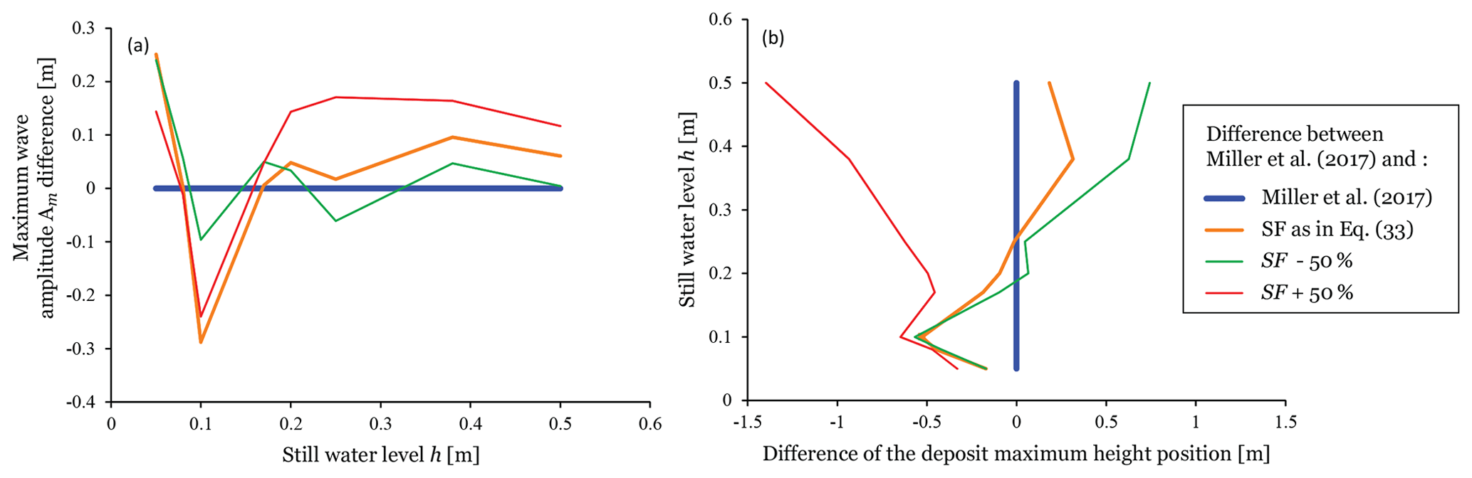
Figure 2 (a) Graph showing the difference between the A_m values from Miller et al. (2017) and Miller et al. (2017) (blue line) and the A_m values from the numerical simulation using different values in Eq. (33). Note that the value used in Eq. (33) (red line) is not the best-fitting curve. (b) Graph showing the difference between the positions of the apex of the landslide deposits observed in Miller et al. (2017) and Miller et al. (2017) (blue line) and the positions obtained from the numerical simulations.

3.2 Computation time

All the simulations are performed on a conventional computer. It is an Acer Aspire V17 Nitro. The computations are performed on an Intel^® Core™ i7-7700HQ CPU at 2.80 GHz with 16 GB of RAM. For a complete simulation, i.e. a simulation that includes landslide and wave propagation, for a duration of 30 s (as presented in Fig. 9), the computation time is 16 650 s. The cell size is 0.01 × 0.01 m, and the grid size is 45.2 m × 2.1 m (949 000 cells).

4 Results

The landslide and the tsunami models are computed in two dimensions (x and y), whereas the results, such as the landslide thickness or the water elevation, can be represented visually in the third dimension (z) or, in other words, in 2.5D, as illustrated in Fig. 3.

In this study, everything is computed in two dimensions, but the interpretations and the presentation of the results is performed through longitudinal cross sections across the centre of the numerical flume (Fig. 4). Figure 4 illustrates the generation of the wave: at 0 s, the landslide impacts the water; at 0.3 s, the landslide velocity is greater than the water velocity and the momentum is transferred; at 0.6 s, the front of the slide starts to stop while the back continues to transfer the momentum to the water; at 0.9 s, the momentum transfer is nearly completed and the wave propagates along the flume. The simulation does not reproduce perfectly the real generation behaviour due to the shallow-water approximations that do not model the impact crater as observed in Miller et al. (2017).

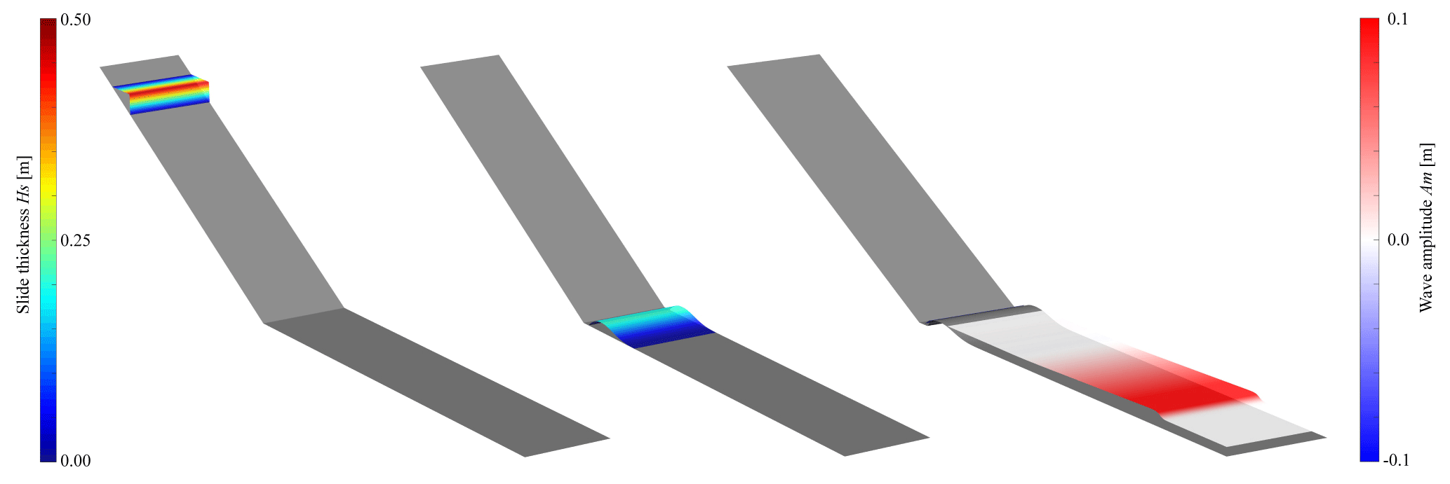
Figure 3 Numerical representation in 2.5D of the near-field section of the flume with water depth h= 0.2: (left) initial condition of the landslide (water level not displayed), (centre) landslide deposit (water level not displayed) and (right) landslide deposit (not coloured) with the generated wave.

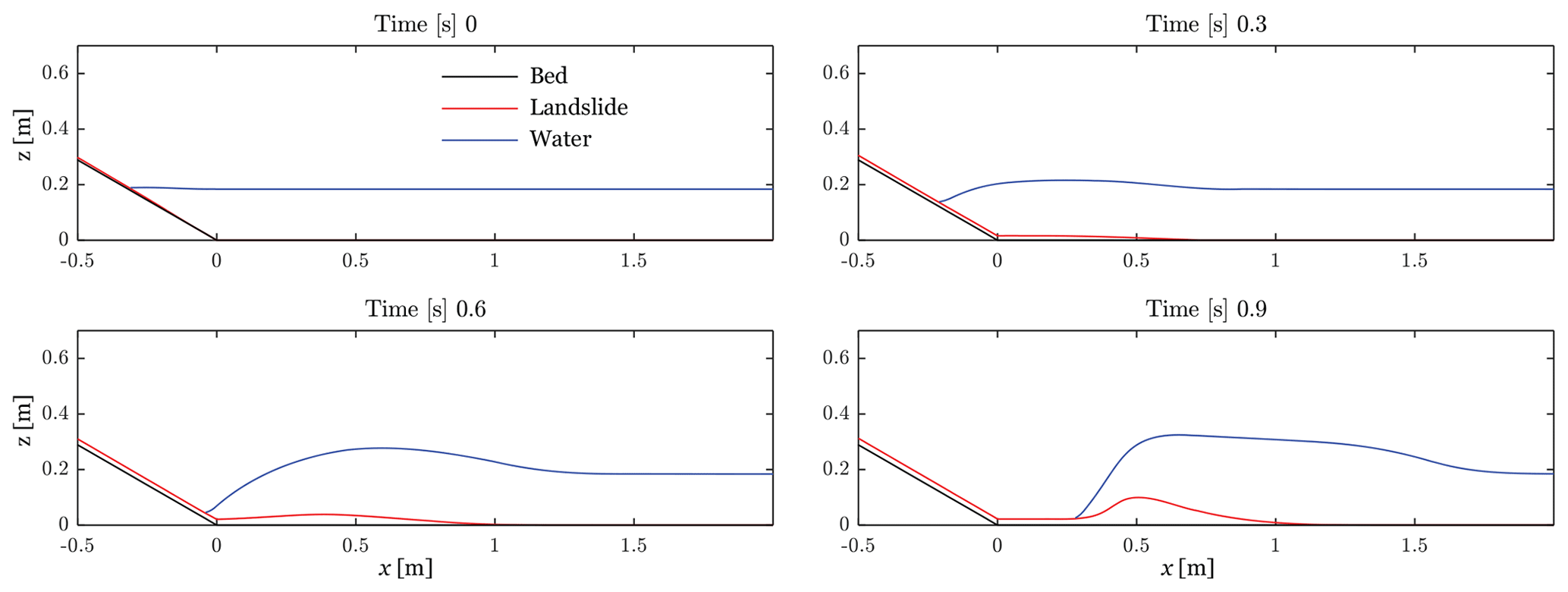
Figure 4 Cross section of the landslide and water surface during numerical simulation of the generation of the wave.

4.1 Landslide

This section presents the results concerning the granular landslide. Furthermore, this section discusses the behaviour of the landslide propagation using different rheological laws and the effect of the water depth on the landslide deposit.

4.1.1 Dry case

The dry case investigates the propagation of the granular material using various rheological laws. The rheological laws implemented herein are the Voellmy, Coulomb (flow with isotropic and anisotropic internal stresses) and Bingham rheological models. The velocities, the thicknesses and the deposit shapes obtained through the numerical simulation are compared to those data obtained from the physical experiment to identify and select the best solution.

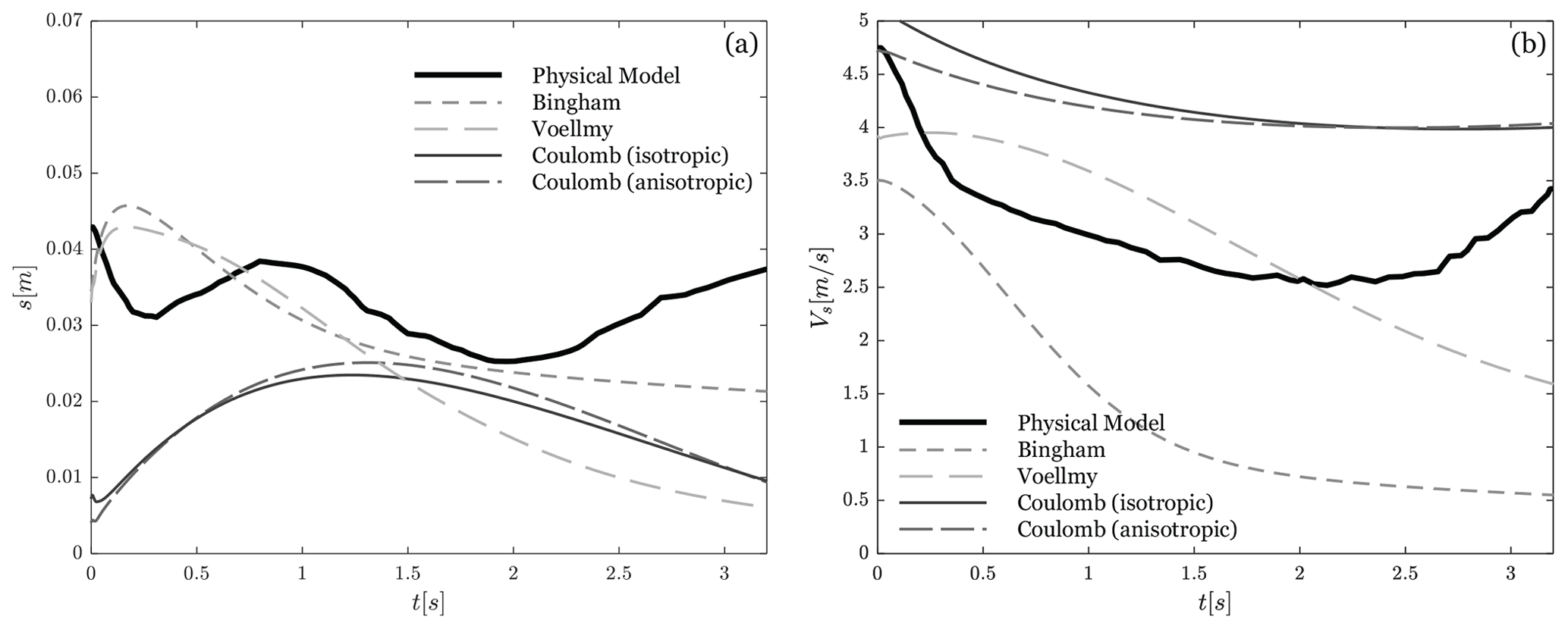
Figure 5 Landslide properties at impact (numerical equivalent location of Cam 1) with a still-water depth h of 0.25 m. (a) Time series of slide thickness for different rheological laws (numerical model) compared with the mean thickness in the physical model. (b) Time series of depth-averaged slide velocity for different rheological laws (numerical model) versus the mean velocities in the physical model (modified from Miller et al., 2017).

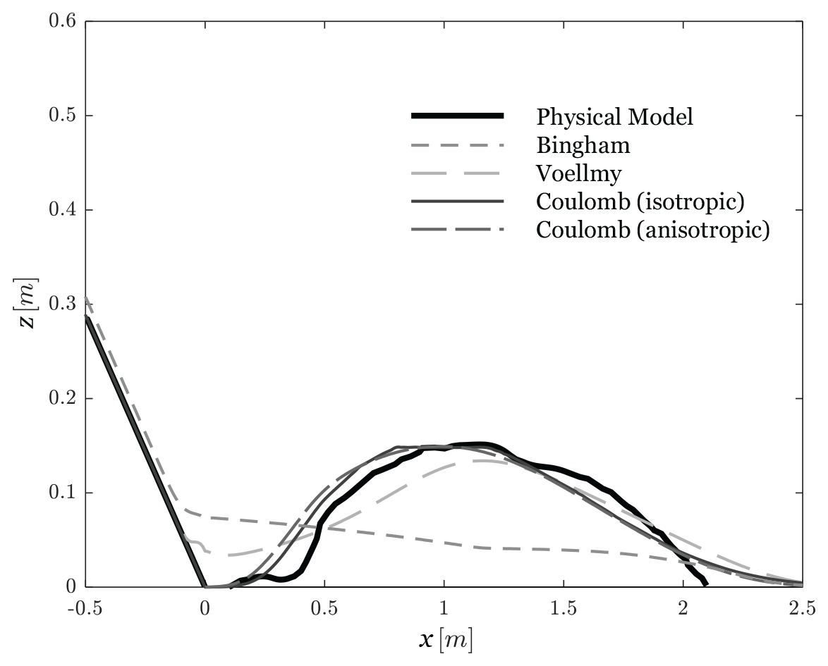
Figure 6 Cross section of the landslide deposit using different rheological laws compared with the deposit in the physical experiment.

The Bingham rheology is set by best fit with a shear zone relative thickness d₁ of 0.6, a yield stress T₀ of 12 Pa and a dynamic viscosity μ of 1.6 Pa s.

Concerning the Voellmy rheology, the determination of the turbulence coefficient ζ is performed by trial and error to obtain the best fit (back analysis). Thus, the turbulence coefficient ζ, as described in Hungr and Evans (1996) and in McDougall (2006), is set to 250 m/s². The bed friction angle φ_bed of 22^∘, given in Miller et al. (2017), is reduced to 11^∘. Indeed, the Voellmy rheology uses significantly lower values (Hungr and Evans, 1996). This study uses the same ratio (∼0.5) between “classical” φ_bed and “Voellmy” φ_bed as the one presented in Hungr and Evans (1996) for cases with similar friction angles and turbulence coefficients (Voellmy φ_bed= 11^∘).

Regarding the two Coulomb models, we use the bed friction angle φ_bed of 22^∘, as measured in the physical experiment (Miller et al., 2017). In addition, the anisotropic Coulomb rheological model considers the internal friction angle φ_int, which is 33.7^∘ (Miller et al., 2017). All the aforementioned parameters are summarized in Table 1.

Table 1 Rheological parameters used for the different rheological laws.

In Miller et al. (2017), the velocity and the thickness of the landslide at impact are estimated through high-speed camera footage analysis with a still-water depth h of 0.25 m. To measure the same variables of the simulated granular flow, the values are recorded using a corresponding window (Cam 1, Fig. 1).

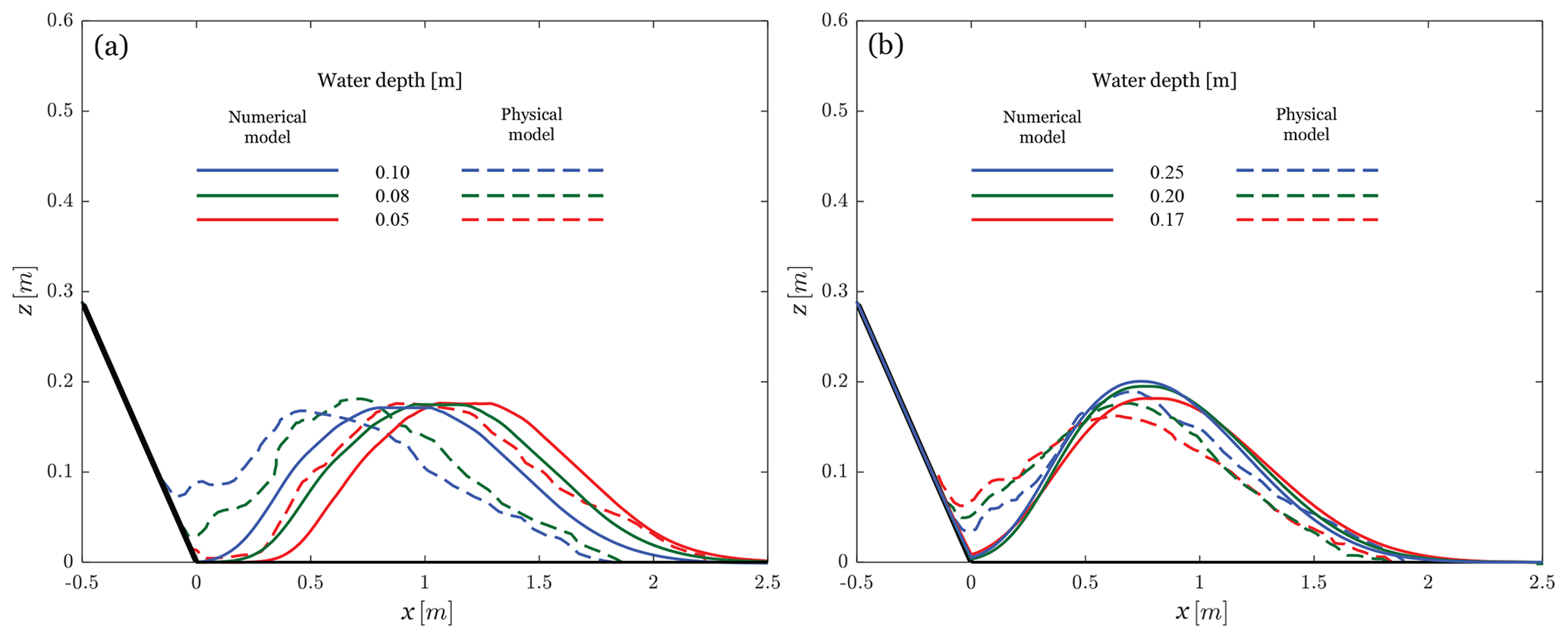
Figure 7 Cross section of the granular flow deposit for different still-water depths h (0.05 to 0.25 m) (modified from Miller et al., 2017).

Figure 5 shows the temporal evolution of the flow thickness and velocity captured at the numerical equivalent location of Cam 1 (Fig. 1). The numerical models do not fit the physical simulation very well. This poor fit can be explained by the diffuse nature of a granular flow boundary that is not replicable by the shallow-water assumption (continuum mechanics) and by the absence of expansion in the numerical moving mass. Nevertheless, the results from the numerical and physical models are close enough to validate globally the different numerical models without allowing their differentiation.

Figure 8 Cross section of the granular flow deposit for two still-water depths h (0.38 and 0.5 m). For comparison, the red line illustrates the landslide deposit for a still-water depth h of 0.38 m without momentum transfer (modified from Miller et al., 2017).

Consequently, analysing the deposit (Fig. 6) is the way to identify the best-fitting rheological model. The Bingham rheological model does not correctly reproduce the shape of a granular deposit. The Voellmy model performs better than the Bingham model in this respect, but in comparison with the two Coulomb frictional models, the Voellmy model is not satisfactory. Indeed, the two Coulomb rheological models (anisotropic and isotropic) fit the best with the observed deposit, which was expected because frictional rheological laws are typically developed to describe granular flows. The rear parts of the deposits are correctly located, whereas the fronts are slightly too distant. However, this imperfection is negligible and could be attributed to numerical diffusion. The deposit simulated with the isotropic Coulomb model is slightly closer to the real deposit than that simulated with the anisotropic model; this method has the advantage of being simple (only the bed friction angle φ_bed is implemented).

Since the velocities and the thickness are of a realistic magnitude, the deposit shapes of the two Coulomb models correctly reproduce the real case. Furthermore, due to the ease of implementation, the isotropic Coulomb model is the finally chosen rheological model. In Sect. 4.1.2, this model is used to study the wet cases.

4.1.2 Wet cases

This section investigates the interaction between the landslide and the water. More precisely, this section investigates the effect of the momentum transfer on the deposit shape for different water levels. Figure 7a shows the results for still-water depths h of 0.05, 0.08 and 0.1 m. The deposits resulting from the numerical simulation (solid lines) are compared with the physical-model observations (dashed lines), which shows a rather good similarity when focusing on the height of the piles. The numerical deposition shape for a still-water depth h of 0.05 m fits well the physical shape, also regarding the spread. Concerning still-water depths h of 0.08 and the 0.1 m, the numerical granular flows stop further than the real flows.

At still-water depths h of 0.17, 0.2 and 0.25 m (Fig. 7b), the numerical and physical results are in good agreement; however, the “tails” and the apexes of the deposits are located slightly farther away in the numerical simulation.

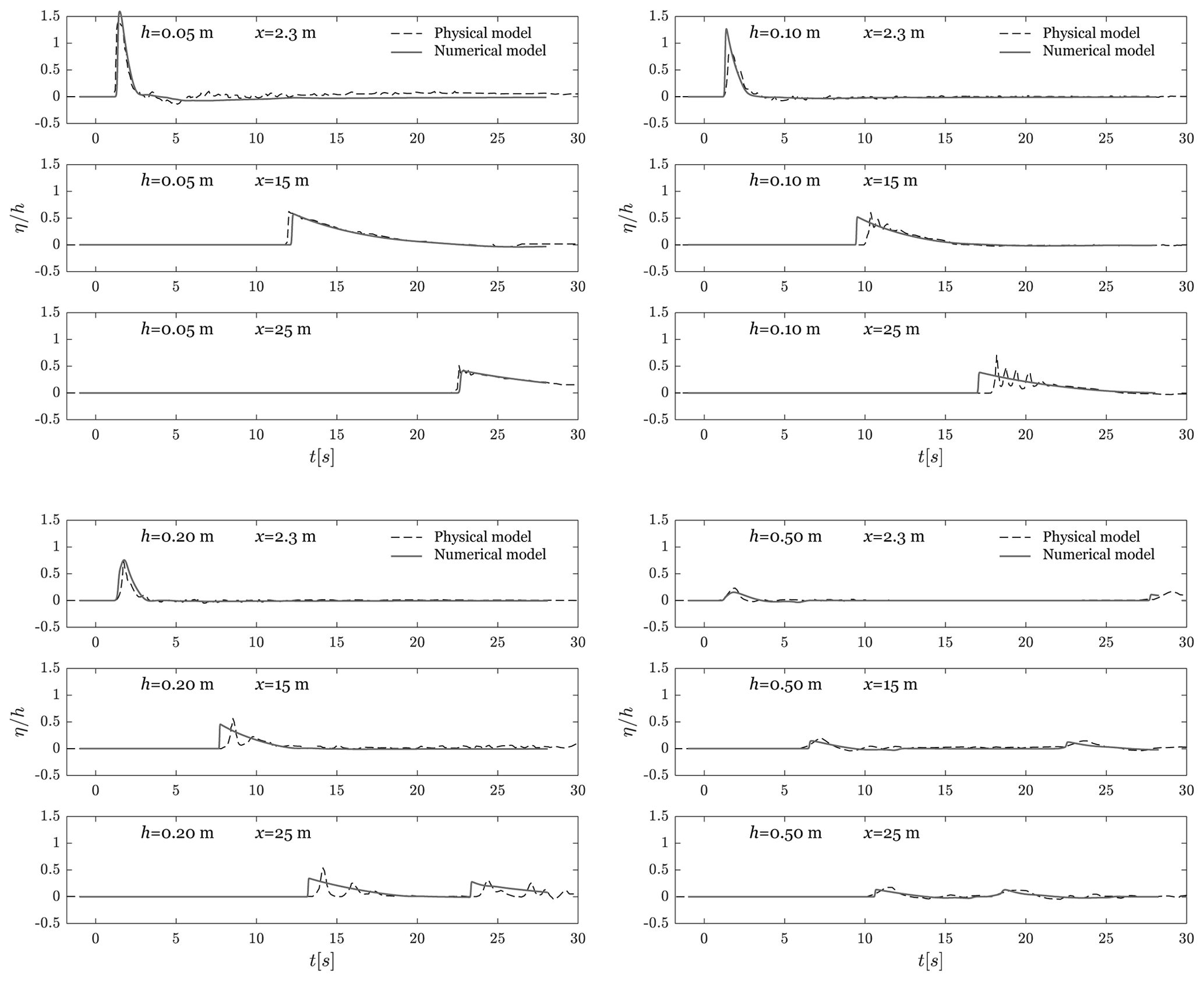
Figure 9 Time series of the relative water surface elevation $\mathit{\eta }/h$ for different still-water depths h (0.05, 0.10, 0.20 and 0.50 m) observed at different wave probes or gauges (2.3, 15 and 25 m) (modified from Miller et al., 2017).

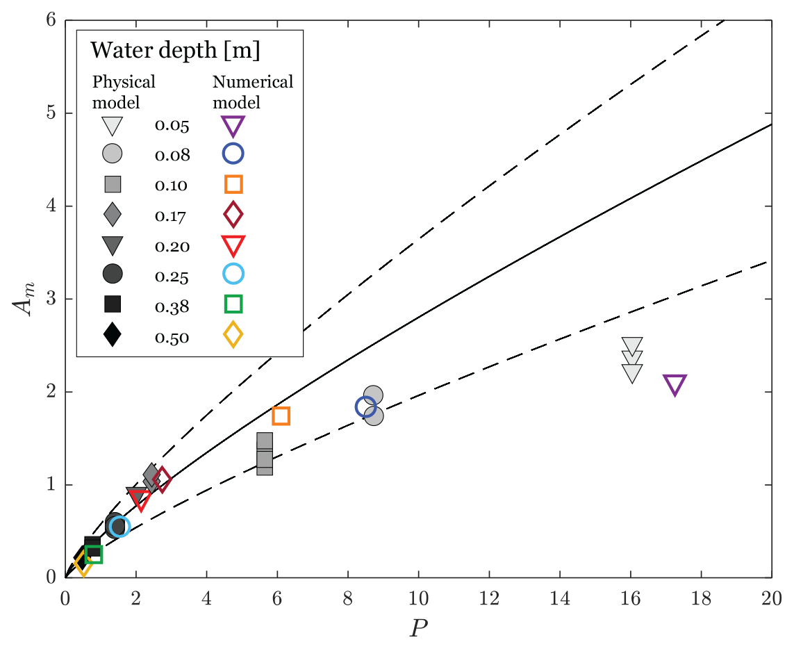
Figure 10 Maximum relative wave amplitude A_m as a function of the impulse product parameter P: A_M from Eq. (39) (solid line), A_M from Eq. (39) ±30 % (dashed lines), data from the physical model (Miller et al., 2017) (solid shapes) and data from the numerical simulation (this study) (hollow shapes).

In contrast, for still-water depths h of 0.38 and 0.5 m (Fig. 8), the deposit shapes obtained by the numerical simulations stop slightly ahead of the real deposits. Nevertheless, the deposits are of equivalent heights.

The momentum transfer acts correctly on the granular flow as the global correspondence between the numerical and physical deposition pattern is good. In fact, it is the combination of the momentum transfer (Eqs. 31 and 32) with the relative density ρ (Eqs. 7–11) that performs well. This is highlighted by the simulated granular landslide without momentum transfer, which travels excessively far (Fig. 8, red line). The travel distance in this case is even greater than that in the dry case (the result of the isotropic Coulomb model presented in Fig. 6) due to the effect of the relative density ρ. Indeed, the “drop in density” when the granular flow enters the water body reduces the total retarding stress Tin particular (Eqs. 10 and 11; alongside PT (Eq. 9) and GR (Eq. 8), which is negligible on flat surfaces). It is worth noting that without momentum transfer or relative density, the model would lead to the same deposit as in the dry case.

4.2 Wave

This section investigates the momentum transfer between the slide and the generated wave This effect is analysed for different still-water depths h (0.05, 0.1, 0.2 and 0.5 m) through probes located at different distances from the bottom of the slope (2.3, 15 and 25 m; Fig. 9). Concerning the case with the smallest still-water depth (h= 0.05 m), the numerical simulation reproduces the wave observed in the physical experiment well in terms of amplitude and timing at each probe. Indeed, the percentages of deviation of the simulated wave compared to the physical one at the probes are +9.7 %, −3.5 % and −6.1 %, respectively. Note that the simulated wave is taller than the real wave in the very near field (2.3 m gauge). For a still-water depth h of 0.1 m, the timing is good at the 2.3 m gauge, but, as previously described, the numerical wave is taller (+51 %). Concerning the gauges at 15 and 25 m, the wave celerity is faster and its amplitude is smaller in the numerical simulation than in the physical experiment (−11.9 % and −41.2 %, respectively). Moreover, the wave train observed in the physical model is non-existent in the numerical model. Except for the equivalence in amplitude in the near field, the same observations apply for a still-water depth h of 0.2 m, with respective deviation of +4.8 %, −16.2 % and −25 %. For a still-water depth of 0.2 m, a reflected wave is present at the 25 m gauge after approximately 23 s. The numerically simulated wave arrives slightly earlier than the observed wave. Concerning the case of a still-water depth h of 0.5 m, the simulated wave is smaller than the real wave (−29.7 %, −13.9 % and −12.3 %, respectively) and the reflected wave (at 28, 23 and 18 s) is visible at the three gauge locations with a good correspondence in terms of time. Those discrepancies are due to the approximations inherent to the shallow-water equations and are discussed in Sect. 4.3. In particular, the non-reproduction of train waves is due to the absence of frequency dispersion.

4.2.1 Impulse product parameter

Heller and Hager (2010) proposed a relationship between the landslide characteristics and the near-field maximum amplitude of the generated wave through the concept of the impulse product parameter P. The impulse produce parameter includes the governing parameters related to the landslide and the still-water depth. The maximum wave amplitude can be predicted as a function of P through Eq. (37). This approach is relevant to our study because it inherently considers the momentum transfer occurring during wave generation. The following values are captured at the impact zone (Cam 1, Fig. 1) for the sliding mass and in the near-field area for the wave. The relative maximum near-field wave amplitude A_m is defined by the following expression:

$$\begin{array}{}\text{(34)}& A_{\mathrm{m}}=\mathrm{0.25}{\mathit{Fr}}^{\mathrm{1.4}}{S}_{\mathrm{R}}^{\mathrm{0.8}},\end{array}$$

where S_R is the relative landslide thickness and Fr is the Froude number, which are defined as follows:

$$\begin{array}{}\text{(35)}& {\displaystyle }{S}_{\mathrm{R}}=s_{\max }/h,\text{(36)}& {\displaystyle }\mathit{Fr}=u_{\mathrm{s}}/\sqrt{\left(gh\right).}\end{array}$$

The relationships between P, Fr and S_R were found empirically through a large set of tests based on different landslide setups (Fritz et al., 2004). The impulse product parameter P defined by Heller and Hager (2010) is expressed as follows:

$$\begin{array}{}\text{(37)}& P=Fr{S}_{\mathrm{R}}^{\mathrm{1}/\mathrm{2}}{M}^{\mathrm{1}/\mathrm{4}}{\left\{\cos \left[\left(\mathrm{6}/\mathrm{7}\right)\mathit{\alpha }\right]\right\}}^{\mathrm{1}/\mathrm{2}},\end{array}$$

where M is the relative landslide mass. This is defined by the following expression:

$$\begin{array}{}\text{(38)}& M=m_{\mathrm{s}}/\left({\mathit{\rho }}_{\mathrm{w}}b{h}^{\mathrm{2}}\right),\end{array}$$

where m_s is the landslide mass and b is the flume width. The near-field relationship between P and A_m is defined as follows (Heller and Hager, 2010):

$$\begin{array}{}\text{(39)}& A_{\mathrm{M}}={\displaystyle \frac{\mathrm{4}}{\mathrm{9}}}{P}^{\mathrm{4}/\mathrm{5}}.\end{array}$$

Figure 10 shows this relationship with the results of Miller et al. (2017) alongside the results of the present study. The two dashed lines represent the same relationship ±30 %. A large set of data collected in flume experiments (Fritz et al., 2004; Heller and Hager, 2010) falls between those limits for P<9.

The near-field relationships between P and A_m obtained in the present study correspond well with those obtained by Miller et al. (2017) (Fig. 10). The two different trends observed for P < 5 (h= 0.17, 0.20, 0.25, 0.38 and 0.5 m) and P > 5 (h= 0.05, 0.08 and 0.1 m) are also present in both physical experiments and numerical simulations. The decreasing maximum relative wave amplitudes A_m of the second set (h= 0.05, 0.08 and 0.1 m) obtained in the physical experiments have been explained by scale effects (Heller, 2011; Miller et al., 2017) and braking bores (Miller et al., 2017). On the other hand, for P < 9 (as originally presented in Heller and Hager, 2010), the results of this study are located within a range of ±30 %.

4.3 Discussion

The numerical model displays a taller wave in the near field, which can be explained by the fact that the model does not reproduce the breaking of the wave. This lack also implies that the model cannot consider the impact crater as long as the steepness of the water surface is not steeper than sub-vertical. This discrepancy is inherent to the shallow-water model and its two-dimensional nature.

The physical experiments produce wave trains for water levels of 0.1 and 0.2 m. This phenomenon is not reproduced by the numerical model because of the absence of breaking in the unstable numerical waves (Miller et al., 2017; Ruffini et al., 2019), along with the lack of modelling frequency dispersion (Ruffini et al., 2019). These mismatches are due to the incomplete physics inherent to shallow-water-equation approximations.

On the other hand, the fronts of the waves are very different. The “excess” volume of water at the front of the numerical wave is also partially explained by the lack of energy dissipation that would occur during breaking. On average, the simulated water level located at the wave train “matches” the trough and the crests. For those cases, the imperfect reproductions are, however, sufficiently close in terms of celerity and volume to be considered relevant. This consideration was in addition confirmed by the good match of the reflected wave (e.g. Fig. 9, h= 0.2, x= 25, 23 s).

The general observation of the evolution of the wave (Fig. 9) shows that the decay occurring in the physical experiment is present in the numerical simulation. This fact also strengthens the general validity of the whole numerical model.

Inherently, as the impulse product parameter values obtained through a wide set of experiments (Heller and Hager, 2010; Miller et al., 2017) fall into an envelope of ±30 %, our near-field results, which also fall into these limits, strongly confirm the validity of our model and our momentum transfer approach. However, the scale effects and the breaking bores affecting the maximum relative water amplitude A_m for P > 5 performed in laboratory experiments cannot explain the similar effect observed in the numerical results as phenomena such as surface tension, frequency dissipation and breakers were not implemented in the numerical model.

5 Conclusions

This study aimed to validate our two-layer landslide-generated tsunami numerical model, based on non-linear shallow-water equations, particularly concerning the momentum transfer between the landslide and the water. This is performed through the reproduction of the physical experiments conducted by Miller et al. (2017). A dry case is simulated to document the behaviour of the landslide propagation model using different rheological laws. In addition, a wet case is reproduced to investigate the influence of different still-water levels on both the landslide deposit and the generated waves.

The dry case shows that the two Coulomb rheological models (flow with isotropic or anisotropic internal stresses) correctly reproduce the deposit observed in the physical model studied by Miller et al. (2017). The isotropic Coulomb model is the simplest and easiest to implement and is chosen to study the wet case.

The numerical simulation of the wet case investigates the abilities of the model to correctly handle momentum transfer. This case focuses on both the effect of the water on the landslide deposit and the effect of the landslide on the resulting wave. These effects are investigated through different water levels, and it appears that the landslide deposit obtained by the numerical simulations fits well with the physical-model observations. On the other hand, the numerical waves behave similarly to the waves in the physical model. Despite imperfections due to the limitations inherent to the non-linear shallow-water equations (no impact crater, no wave breaking), the combined results from investigating these two effects permits us to consider that, overall, the model simulates relatively well the complex phenomena occurring during the interaction between the landslide and the water. In addition, the choice to transfer the momentum through the simple perfect collision principle is verified to be relevant.

A comparison involving the impulse product parameter particularly highlights that our model satisfactorily reproduces the physical experiment of Miller et al. (2017). The values of A_m versus P presented in Heller and Hager (2010) are based on their 211 experiments in addition to 137 experiments performed by Fritz (2002) and 86 by Zweifel (2004). Hence, the validity of our model is further strengthened by the fact that the results of our model also fit reasonably well (±30 %) with those experiments.

Finally, we consider our model a tool of choice for the assessment of landslide-generated tsunami hazards considering the complexity of the phenomenon reproduced, the acceptable reproduction of the laboratory experiments, and the possibility of performing multi-scenario studies thanks to its efficiency and ease of use.

Appendix A: Notation

Description
Am	maximum measured wave amplitude [m]
AM	theoretical maximum wave amplitude in the near field [m]
B	bed elevation [m]
b	flume width [m]
C	Chézy coefficient [–]
d1	shear layer relative thickness [–]
F	flux vector in x direction [–]
Fr	Froude number [–]
G	flux vector in y direction [–]
g	gravitational acceleration [m/s2]
GR	driving component of gravity [Pa]
H	layer depth [m]
h	still-water level [m]
hmin	minimum water thickness (ultrathin layer) [m]
Hs	landslide thickness [m]
Hsa	landslide thickness after collision [m]
Hsb	landslide thickness before collision [m]
Hw	depth of the water [m]
Hwa	depth of the water after collision [m]
Hwb	depth of the water before collision [m]
K	earth pressure coefficient [–]
LF	Lax–Friedrichs scheme
M	relative landslide mass [–]
ms	landslide mass [kg]
MTs	momentum transfer (water to slide) [Pa]
MTw	momentum transfer (slide to water) [Pa]
n	Manning roughness coefficient [–]
PT	pressure term [Pa]
P	impulse product parameter [–]
Re	Reynolds number [–]
Retr	Re threshold [–]
S	source term [–]
SR	relative landslide thickness [–]
SF	shape factor for momentum transfer [–]
smax	maximum landslide thickness [m]
T	total retarding stress [Pa]
T0	yield stress [Pa]
U	solution vector [–]
u	velocity vector component in x direction [m/s]
us	landslide velocity in x direction [m/s]
usa	landslide velocity in x direction after collision [m/s]
usb	landslide velocity in x direction before collision [m/s]
uw	water velocity in x direction [m/s]
uwa	water velocity in x direction after collision [m/s]
uwb	water velocity in x direction before collision [m/s]
v	velocity vector component in y direction [m/s]
V	full velocity vector [m/s]
vs	landslide velocity in y direction [m/s]
vw	water velocity in y direction [m/s]
x	longitudinal coordinate [m]

Description
y	transverse coordinate [m]
z	vertical coordinate [m]
α	bed slope angle [∘]
Δt	time step [s]
η	wave amplitude [m]
μs	landslide dynamic viscosity [Pa s]
μw	water dynamic viscosity [Pa s]
ξ	turbulence coefficient [m/s2]
ρ	apparent density [–]
ρs	landslide bulk density [kg/m3]
ρsa	landslide bulk density after collision [kg/m3]
ρsb	landslide bulk density before collision [kg/m3]
ρw	water density [kg/m3]
ρwa	water density after collision [kg/m3]
ρwb	water density before collision [kg/m3]
φbed	bed friction angle [∘]
φint	internal friction angle [∘]