DebrisFlow Predictor: an agent-based runout program for shallow landslides

Credible models of landslide runout are a critical component of hazard and risk analysis in the mountainous regions worldwide. Hazard analysis benefits enormously from the number of available landslide runout models that can recreate events and provide key insights into the nature of landsliding phenomena. Regional models that are easily employed, however, remain a rarity. For debris flows and debris avalanches, where the impacts may occur some distance from the source, there remains a need for a practical, predictive model that can be applied at the regional scale. We present, herein, an agent-based simulation for debris flows and debris avalanches called DebrisFlow Predictor. A fully predictive model, DebrisFlow Predictor employs autonomous subroutines, or agents, that act on an underlying digital elevation model (DEM) using a set of probabilistic rules for scour, deposition, path selection, and spreading behavior. Relying on observations of aggregate debris flow behavior, DebrisFlow Predictor predicts landslide runout, area, volume, and depth along the landslide path. The results can be analyzed within the program or exported in a variety of useful formats for further analysis. A key feature of DebrisFlow Predictor is that it requires minimal input data, relying primarily on a 5 m DEM and user-defined initiation zones, and yet appears to produce realistic results. We demonstrate the applicability of DebrisFlow Predictor using two very different case studies from distinct geologic, geomorphic, and climatic settings. The first case study considers sediment production from the steep slopes of Papua, the island province of Indonesia; the second considers landslide runout as it affects a community on Vancouver Island off the west coast of Canada. We show how DebrisFlow Predictor works, how it performs compared to real world examples, what kinds of problems it can solve, and how the outputs compare to historical studies. Finally, we discuss its limitations and its intended use as a predictive regional landslide runout tool. DebrisFlow Predictor is freely available for non-commercial use.

1 Introduction

Mountains occupy 30.5 % of the global land surface (Sayre et al., 2018), provide much of the global water supply and critical economic resources, and directly support hundreds of millions of people around the world. Steep rugged mountain slopes, however, are also responsible for some of the world's deadliest hazards, threatening infrastructure and causing the loss of thousands of lives annually (on average) (Froude and Petley, 2018).

Debris flows and debris avalanches are potentially destructive, rapid to extremely rapid landslides that tend to travel considerable distance from their source. Interaction between debris flows and objects, resources, or people at distal points along their travel path results in a potentially unexpected and dangerous mountain hazard. One of the critical challenges to overcome with respect to debris flow hazards is therefore the credible prediction of size, runout, and depth.

Debris flow runout behavior is controlled by topography, geology (surficial and bedrock), rheology, land use, land cover, water content, and landslide volume. Modeling approaches for predicting debris flow runout have included empirical methods such as total travel distance (Corominas, 1996; VanDine, 1996) or limiting criteria (Iverson, 1997; Benda and Cundy, 1990; Berti and Simoni, 2014), volume balance methods (Fannin and Wise, 2001; Guthrie et al., 2010), analytic solutions and continuum-based dynamic models (Hungr, 1995; O'Brien et al., 1993; McDougall and Hungr, 2003; Rickenmann, 1990; Gregoretti et al., 2016; Hussin, 2011), and cellular automata (Guthrie et al., 2008; Tiranti et al., 2018; Segre and Deangeli, 1995; D'Agostino et al., 2003).

A limited number of models have been applied regionally (Chiang et al., 2012; Guthrie et al., 2008; Horton et al., 2013; Mergili et al., 2015), in part due to the complexity of data inputs. Analytical models in particular, while producing excellent results, are frequently complex and can require back analyses to determine model parameters. Hussin (2011), for example, successfully recreated a channelized debris flow in the southern French Alps but also found that the model results were sensitive to small changes in the entrainment coefficient, turbulent coefficient, friction coefficient, and the digital elevation model (DEM) itself. Adjustments to model parameters can require considerable expertise and complicate the predictive value of the models if applied regionally.

There remains a need for a widely accessible debris flow model that produces credible results with limited inputs.

Guthrie et al. (2008) created a regional landslide model intended to provide evidence that the occurrence of the rollover effect in landslide magnitude–frequency distributions was primarily a result of landscape dynamics rather than data censoring (or other causes). That model used cellular automata methods wherein individual cells (agents) followed simple rules for scour, deposition, path selection, and landslide spread. The model assumed aggregate behavior of rapid or extremely rapid flow-type landslides based on about 1700 data points from coastal British Columbia (Guthrie et al., 2008, 2010; Wise, 1997). Landslide behavior relied on empirical observations that events exhibit similar scour, deposition, depths, and runout independent of geology, rheology, triggering mechanisms, or antecedent conditions. Simply put, once triggered, debris flows and debris avalanches had behavior that tended to be broadly self-similar. The model itself did a credible job of reproducing landslides across a broad region using limited inputs.

The current authors identified a use case and designed, from scratch using C+ and Extensible Application Markup Language (XAML), the landslide runout model presented herein. DebrisFlow Predictor is a stand-alone agent-based model that requires limited inputs and provides the user with both visualization and analytic capabilities. DebrisFlow Predictor is freely available for non-commercial use (university research groups, for example) and may be downloaded here: http://landing.stantec.com/debris-flow-predictor-download-request.html (last access: 16 March 2021).

This paper explains the basis for DebrisFlow Predictor and provides two very different case studies to demonstrate how it might be applied.

2 Description of the program

DebrisFlow Predictor estimates sediment volume (erosion and deposition) along a landslide path by deploying “agents”, or autonomous subroutines, over a 5 m spatial resolution DEM. The DEM surface provides basic information to each agent, in each time step, that triggers the rule set that comprises the subroutine. In this manner, agents interact with the surface and with other agents. Each agent occupies a single pixel in each time step.

2.1 Agent generation

The user defines a starting location by injecting a single agent (5 m×5 m), a group of nine agents (15 m×15 m initiation zone), or by painting a user-defined initiation zone (unlimited size) as indicated by field morphology. Multiple agents may be generated at the same time using any of these methods or any combination of these methods. DebrisFlow Predictor can automatically create 15 m×15 m initiation zones (nine agents) for each point in an imported point file.

The starting location of a single agent, or a group of connected agents, represents the initiation of a landslide. Each landslide knows which agents that belong to it, whatever the method of initiation.

2.2 Agent mass

Agents follow probabilistic rules for scour (erosion) and deposition at each time step based on the underlying slope. Rules for scour and deposition are independent probability distributions for 12 slope classes (bins), modified from Guthrie et al. (2008) to account for a wider range of slopes than the original study (Table 1). They are based on data gathered for coastal BC by Wise (1997) and by Guthrie et al. (2008, 2010), and the results are inferred to be representative of aggregate debris flow behavior elsewhere. Continuous functions are derived for each slope bin within the model, and the user can choose either the step function, drawing directly from Table 1 or the continuous function (recommended).

Table 1 Basic scour and deposition rules used in DebrisFlow Predictor. Data come from Wise (1997) and Guthrie et al. (2008, 2010).

n/a stands for not applicable.

Agent mass can be refined within the program to allow for regions with thicker or thinner available sediment by using the deposition multiplier, erosion multiplier, or min initiation depth sliders. Deposition multiplier and erosion multiplier sliders act on the scour and deposition results at each time step and are independent of one another. Min initiation depth affects the initial mass when generating agents.

Additional rules for deposition are implemented when agents change cardinal direction. This is a user-defined parameter provided as a substitute for frictional deposition.

In each time step, an agent scours, deposits, then checks its mass balance. Mass balance is recorded by the agent in each time step, and agents are terminated when their mass equals zero.

2.3 Agent path selection

Agents with mass move down slope in successive time steps by calculating the elevations of the Moore neighbors (the surrounding eight squares in a grid), determining the lowest three pixels and moving to the lowest unoccupied pixel of the three (Fig. 1). Should the lowest three pixels be occupied, or should some of the pixels be equal elevation, the agent will merge with one of the cells based on similar internal decision-making rules.

Figure 1 Path selection based on aspect determined by Moore neighbors. Black numbers represent time steps, and white numbers represent actual elevations. Example is from Lake Cowichan on Vancouver Island. Pixel resolution is 5 m.

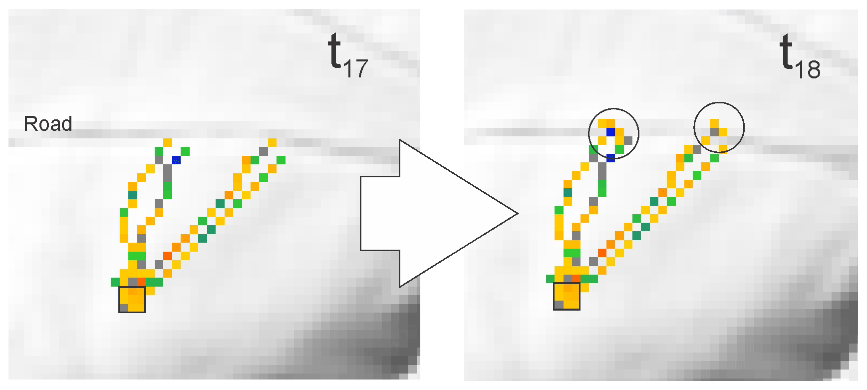
Figure 2 Agent spawning (inside circles) due to a topographic change at a road that is reached in time step 18. Landslide is traveling NE (to upper right corner), and the initiation zone is the 15×15 m square outlined in black.

2.4 Agent spread

Landslide shape and spread (spawning) are described by a probability density function where the mean is centered around the facing direction of an individual agent (accounting for the local slope by way of the Moore neighbors) and the standard deviation, σ, is defined by

$$\begin{array}{}\text{(1)}& \mathit{\sigma }=\left({\left({\displaystyle \frac{m_{\text{MAX}}-m}{m_{\text{MAX}}}}\right)}^n\times \left(\left({\mathit{\sigma }}_{\mathrm{L}}-{\mathit{\sigma }}_{\mathrm{S}}\right)+{\mathit{\sigma }}_{\mathrm{S}}\right)\right),\end{array}$$

where m_MAX=Fan maximum slope, m=DEM slope, n=Skew coefficient, σ_L=Low slope coefficient, and σ_S=Steep slope coefficient.

These are controlled, in turn, by sliders within the program itself that cover a fanning slope limit, above which agents will not spawn, and shape controls that determine how steep and narrow the curve, or alternatively how low and broad the curve, for both steeper and flatter slopes:

• fan maximum slope;

• σ steep slopes;

• σ low slopes;

• skew fanning to low slopes.

Spread is calibrated experimentally based on empirical or observed behaviors of actual landslides. In the absence of observable landslides, the authors recommend using 27^∘.

Spread behavior produces realistic results related to underlying topography such that mass is redistributed at sudden changes in slope (e.g., Fig. 2) or through gradual slope change where landslides tend to widen and deposit.

Spawned agents immediately perform the same rules as other agents in each time step (including the time step in which they were spawned).

2.5 Agent tracking

Each agent leaves behind a track that identifies the changes to the pixel and colors the track according to those changes. This track also provides the visual cue that shows the landslide path.

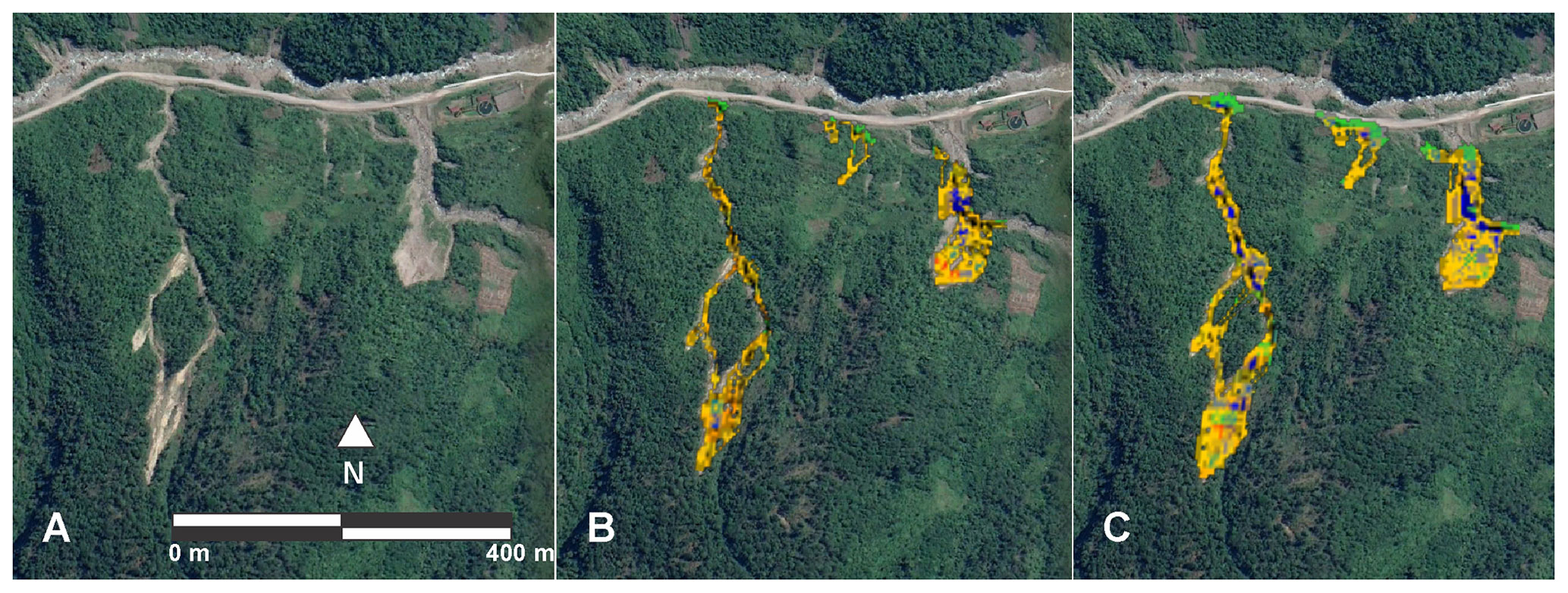
Figure 3 Comparison between historic landslides (a) and modeled landslides from a single run (b), and from 50 runs (the cumulative footprint) (c). Background image © Google Earth. Example is from a site in Indonesia (see case study below).

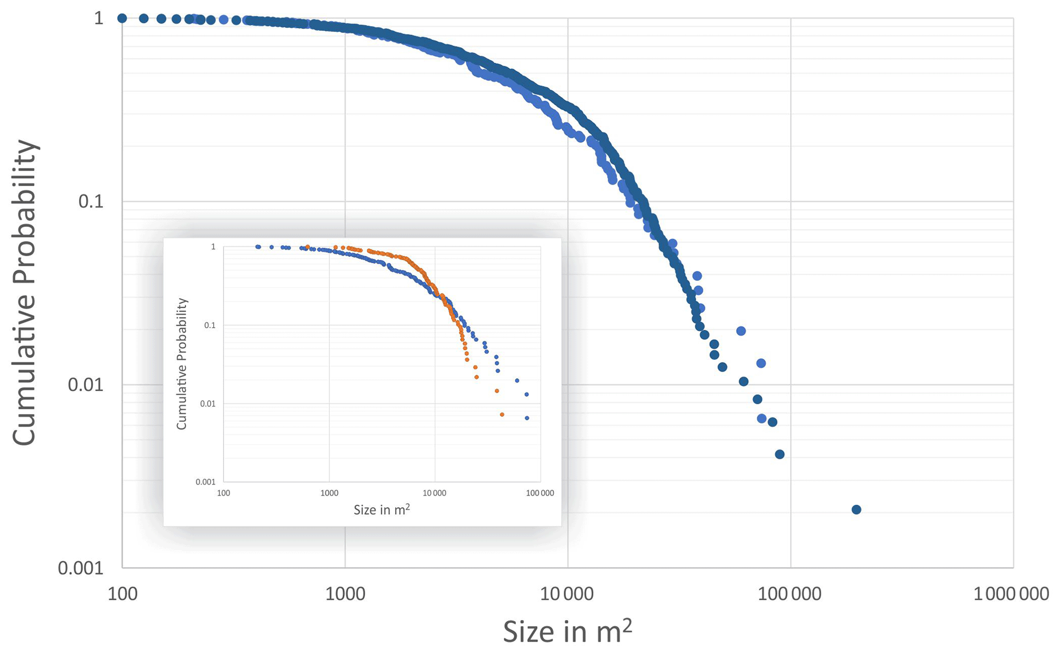
Figure 4 Example of a magnitude–frequency graph of modeled and mapped landslides from a well-calibrated model run and an earlier poorly calibrated model run (inset).

2.6 Model calibration

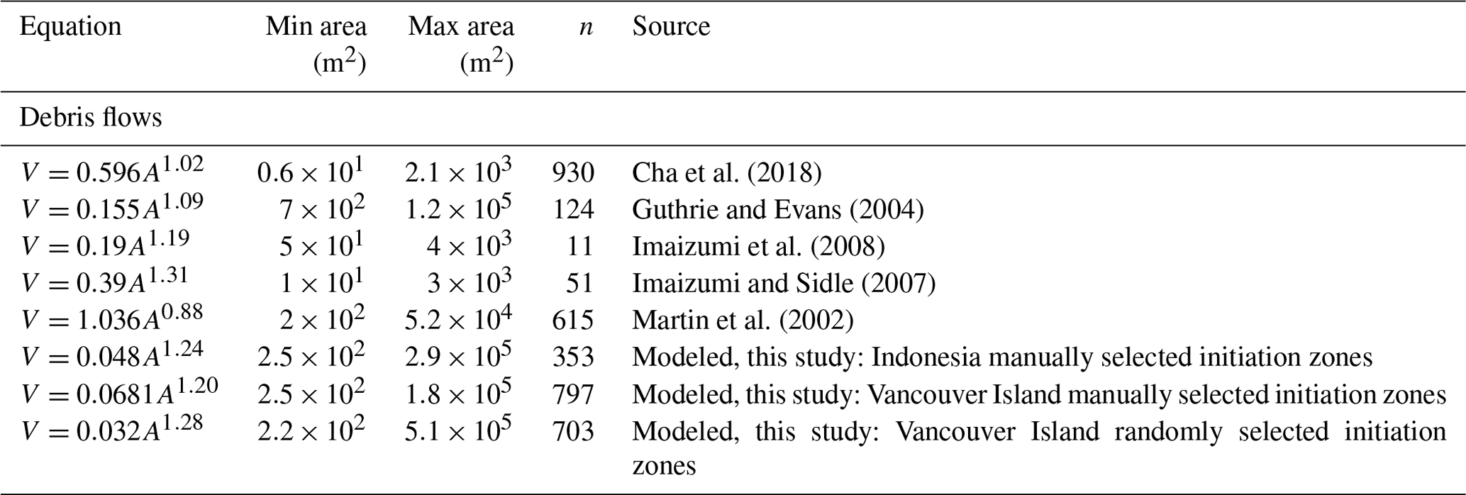
Model calibration is completed iteratively using the controls within the program. The landslide professional runs the model and compares the results to mapped or historical landslides and ground-based evidence for travel distance, scour, and deposition. In addition to field evidence, several other calibration methods may be employed including a visual comparison (Fig. 3), magnitude–frequency comparison of mapped versus modeled landslides (Fig. 4), and comparison of volume–area relationships against known relationships (Fig. 5, Table 2).

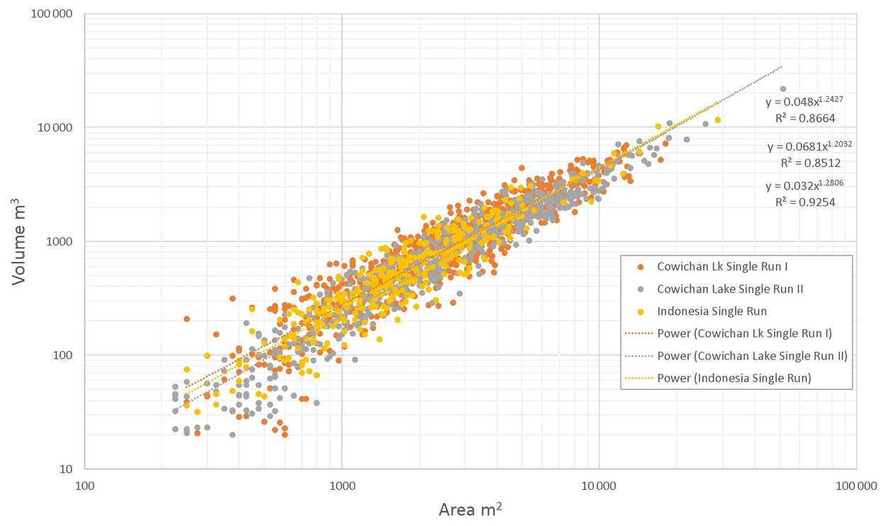
Figure 5 Landslide area–volume relationships for modeled single-run landslides in Indonesia and from Vancouver Island. Data come from case studies described in subsequent sections.

Table 2 Areas and volumes from this study compared with historical studies of debris flow area–volume relationships.

Typically, adjustments are made to the control sliders until better results are realized. This might require several runs. An “inspect” button allows the user to examine the results pixel by pixel and a “one by one” button advances individual agents through single time steps allowing for a much more detailed analysis of results.

By and large, when done by a landslide professional, calibration (qualitative or quantitative) is a relatively straight forward process. The professional must decide whether modeled landslides travel along realistic paths, whether the paths are similar to those of historical events as mapped or as observable in the air photographs, whether the range of deposition and erosion approximates similar events in the same region, and finally, analytically, whether or not the magnitude–frequency and area–volume characteristics are sufficiently similar to mapped characteristics, or justifiably different.

Because DebrisFlow Predictor is both predictive and probabilistic, it may not precisely recreate an existing or historic landslide but instead tries to credibly produce predictions of landslides that may occur on the existing surface. However, the predictive and probabilistic aspect of the program is, in the opinion of the authors, a strength, particularly given that DebrisFlow Predictor includes the ability to model many landslides and compare the range of responses between runs.

2.7 Outputs

DebrisFlow Predictor produces results from a single run, single landslide; single run, multiple landslides; multiple runs, single landslide; or multiple runs, multiple landslides. Following a run or set of runs, each pixel can be queried to provide information about the debris depth (net deposition) at that location, the landslide number, the pixel facing direction, and basic topographic information such as elevation and location. Multiple runs also provide some basic statistics including the number of times a pixel was occupied by an agent, and the minimum and maximum debris depth over all runs.

Each pixel is colored to represent scour or deposition. Red through yellow represent net scour (red being deeper than yellow), and green through blue represent net deposition (blue being deeper than green). Grey colors represent no change, or in the case of multiple runs, they represent no average change in depth (transition zones).

Figure 6 demonstrates the difference in scour and deposition along a landslide path. The reader can see that road(s) tend to accumulate sediment, consistent with observations on Vancouver Island (Guthrie et al., 2010). Similarly, scour on the fill slope side of the road, where it is locally steeper, is also easily observed.

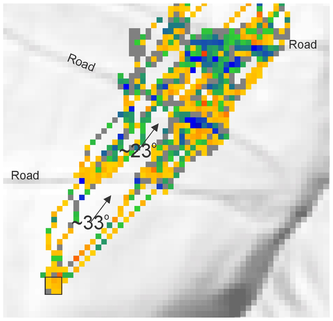
Figure 6 Topographic effects on landslide propagation are easily seen. Agents spawn at and below the road(s), causing the landslide to spread. Approximate average slopes are shown in the figure. This figure is the continuation of the landslide path from Fig. 2. The landslide is moving NE (towards the top right), and the initiation zone is the 15×15 m square outlined in black in the lower left corner.

2.7.1 Export to Excel

Landslide specific information (landslide number, area, volume) can be exported as an Excel file. The output allows the user to analyze magnitude–frequency characteristics of the modeled landslides, including area and volume from the entire footprint, the erosion, and deposition zones, and confirm credible results.

2.7.2 Export to shapefile

Data are easily exported to a shapefile through either an export point function or an export to layer function. The first converts each pixel and associated metadata for each landslide to a point file for analysis in geographic information system (GIS) software, while the second exports the metadata to an existing shapefile, allowing, for example, the user to estimate cumulative sediment contribution to previously mapped polygons.

2.7.3 Export to GeoTIFF

DebrisFlow Predictor exports the modeled landslides as GeoTIFFs to enable viewing in other software and visual comparison with existing ground conditions.

3 Case studies

To better understand how DebrisFlow Predictor performs and how it might be applied, additional results are described in each of two unique case studies below.

3.1 Case study I: debris flows in Papua, Indonesia

3.1.1 Background

Tembagapura is a high alpine town, 2000 m a.s.l., in the Jayawijaya Mountains in the Mimika regency of the province of Papua, Indonesia (Fig. 7). Formed from uplifted and accreted terrains driven by the oblique convergence of the Pacific and Indo-Australian plates (Davies, 2012). Tembagapura is surrounded by steep mountain slopes that regularly produce landslides including debris flows and debris floods. The area above the town is 21.4 km² and constitutes 2646 m of relief.

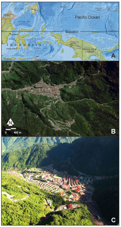
Figure 7 Tembagapura located in the province of Papua, Indonesia. (a) Regional view, yellow star indicates Tembagapura (image © ESRI and National Geographic World Map), (b) vertical image over Tembagapura showing debris flows and debris floods (image © Google Earth), (c) oblique view of Tembagapura in the steep Jayawijaya Mountains.

In 2017, debris floods¹ swept through the town, causing considerable damage, and town authorities sought to better understand the expected magnitude and frequency of debris floods to better mitigate and prepare for future events.

A landslide inventory was conducted using remotely acquired vertical color imagery from 2012, 2016, and 2017. The inventory resulted in 375 mapped landslides (Fig. 8) in the Tembagapura watershed and revealed that landslide evidence had a short persistence time in the dense and verdant vegetation (see Guthrie and Evans, 2007, for a discussion of geomorphic persistence).

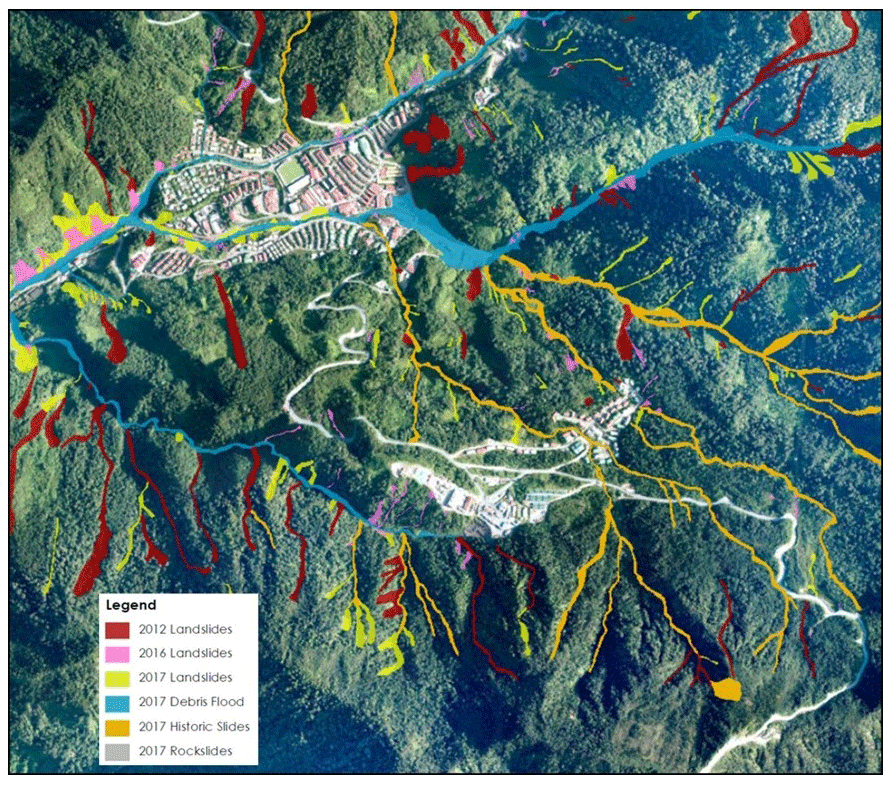
Figure 8 An historical inventory revealed 375 landslides, primarily debris flows, in the slopes surrounding Tembagapura. Years refer to the year of imagery and the background image is a vertical air photograph obtained by the authors.

Rapid weathering and soil formation were inferred to provide a near-infinite sediment supply that moves through the watershed in a “conveyor-belt” type process, whereby weathered rock was transported to the river system and subsequently transported downstream in successively larger floods.

With multiple landslides occurring annually, a relationship describing landslide triggering rainfall was built from the landslide inventory, weather data, and the town records of landslide-causing precipitation events (Fig. 9). In order to supply a debris flood model, the amount of sediment generated by landslides, and thus contributing to the conveyor belt of available sediment, was modeled in DebrisFlow Predictor.

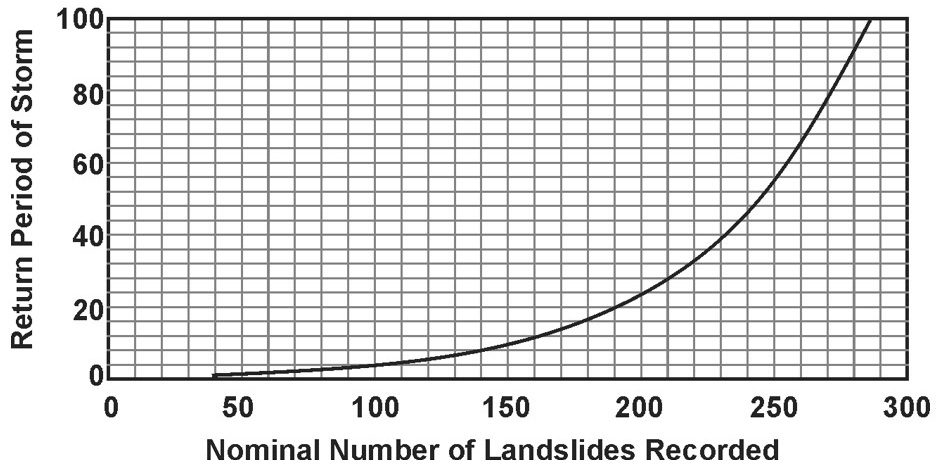
Figure 9 The relationship between landslide occurrence and landslide-generating rainfall at Tembagapura.

3.1.2 Running the model

Within the program, landslides were calibrated visually by first painting head scarps onto an imported shapefile of the historical inventory and a 5 m DEM acquired in 2018 (Fig. 10). The landslide simulation was activated (by toggling the “Go” button) and the results compared visually to mapped landslides (Fig. 11) and on-the-ground results.

Figure 10 Landslide initiation zones painted (yellow) at the estimated source of mapped debris flows (darker line work) in DebrisFlow Predictor.

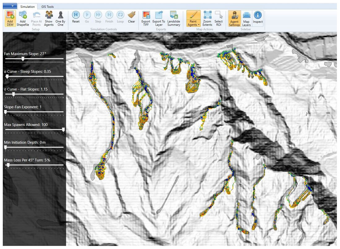
Figure 11 A single run of the landslides whose initiation zones were painted in Fig. 10 above. Colors relate to scour (yellow to red where red is deeper) and deposition (green to blue where blue is deeper).

DebrisFlow Predictor produced morphologically meaningful results when comparing flow paths, scour and deposition regions, divergence, convergence, and runout. In addition, area–volume relationships and the magnitude–frequency statistics between mapped and modeled landslides were plotted similarly (Fig. 12).

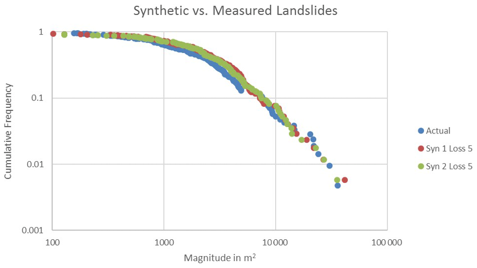
Figure 12 Cumulative magnitude–frequency comparison between mapped and modeled landslides (two runs).

3.1.3 Calculating sediment production

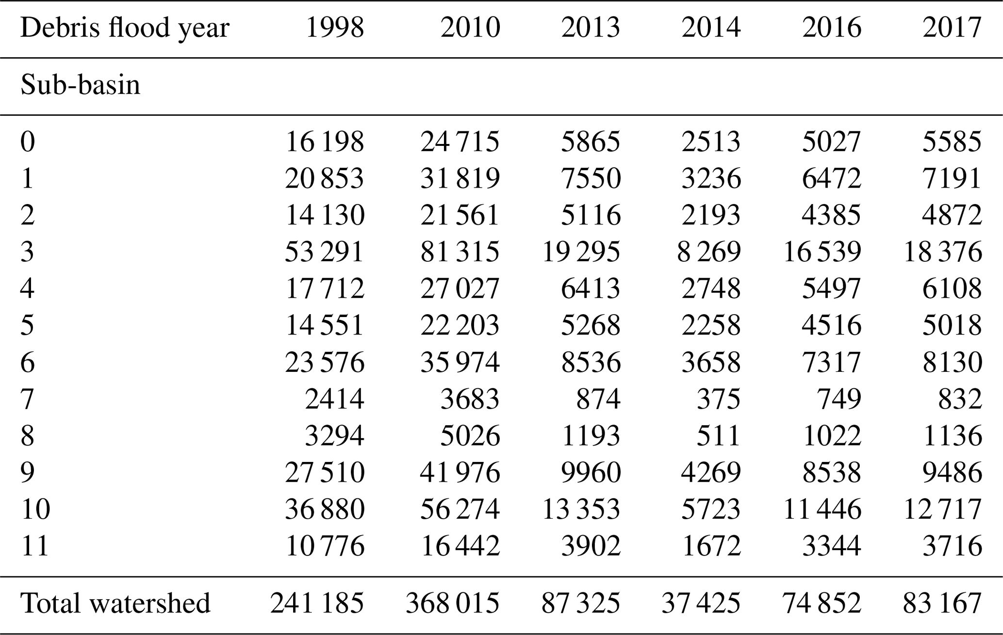
Six significant debris flood producing storms since 1991 were identified based on town records (1998, 2010, 2013, 2014, 2016, and 2017). In order to simulate sediment made available to the conveyor belt system of sediment production during major storms, landslides were randomly generated from susceptible slopes (e.g., Fig. 13) between debris flood years using the relationship from Fig. 9. The sediments mobilized were accumulated into 12 sub-basins for the periods between each significant debris flood (Table 3). A debris flood model (FLO-2D) was then run through the system using the accumulated sediment as a bulking factor and compared to actual events.

Figure 13 Landslides generated from susceptible slopes in DebrisFlow Predictor. Bottom figure shows depths along the landslide path.

Table 3 Accumulated landslide-generated sediment (in m³) between known debris flood years.

Once the modeled debris floods were calibrated against historical events, design floods were determined by bulking the debris flood model (FLO-2D) with sediment estimated in DebrisFlow Predictor for specific storm return periods (Table 4). In this case, sediment was accumulated in the model under the assumption that no debris flood greater than the 5-year event had occurred in the preceding 5 years. The results allowed the user to estimate hydrograph bulking for the 10-, 20-, 25-, 50-, and 100-year events.

Table 4 Accumulated landslide-generated sediment (in m³) by return period of landslide-generating storms.

3.1.4 Case study I: summary

DebrisFlow Predictor successfully simulated debris flows in the steep mountains surrounding Tembagapura. Scour zones were painted using the supplied tool and, for predictive analysis, were created automatically from randomly generated points using an imported shapefile.

The results were used to estimate landslide-generated sediment to the stream network subsequently flushed by periodic debris floods. The model produced morphologically meaningful results and similar magnitude–frequency characteristics to mapped landslides (Fig. 12). The sediment contribution from slopes was easily exported to shapefiles for analysis and summation and ultimately to provide volume estimates for hydrograph bulking in the debris flood model at user-specified design floods.

3.2 Case study II: understanding of risk from debris flows on Vancouver Island

3.2.1 Background

Vancouver Island comprises approximately 31 788 km² of rugged terrain between sea level and 2200 m elevation off the Canadian west coast. Oriented NW–SE, the steep Vancouver Island Ranges form the volcanic backbone of the island. Basalt and andesite are intermixed with marine sedimentary rocks, intruded in turn by granitic batholiths (Yorath and Nasmith, 1995). Pleistocene glaciation carved deep fjords and inlets, and created oversteepened U-shaped valleys that characterize the topography today. Precipitation varies between 700 mm and over 6000 mm yr⁻¹, and landslides are common with rates between 0.007 and 0.096 ${\mathrm{km}}^{-\mathrm{2}}{\mathrm{yr}}^{-\mathrm{1}}$ depending on the regional zone (wet, moderate, dry, and alpine), as identified by Guthrie (2005b). Guthrie (2005b) further observed that more than two-thirds of all landslides below the alpine zone are debris flows.

Cowichan Lake (Fig. 14) is an elongated bedrock-controlled lake on southern Vancouver Island. The lake fills the glacially scoured contact between relatively competent Karmutsen and Bonanza volcanic rock on the south shore, and more erodible volcanic and volcaniclastic rocks of the Sicker Group on the north shore (Guthrie, 2005b). The steep northern slopes of Cowichan Lake lie within the dry zone and subsequently the lower range of landslide occurrence (0.004 ${\mathrm{km}}^{-\mathrm{2}}{\mathrm{yr}}^{-\mathrm{1}}$), modified by the underlying bedrock to as much as 0.008 ${\mathrm{km}}^{-\mathrm{2}}{\mathrm{yr}}^{-\mathrm{1}}$ (1 landslide × 125 km⁻²) (Guthrie, 2005b).

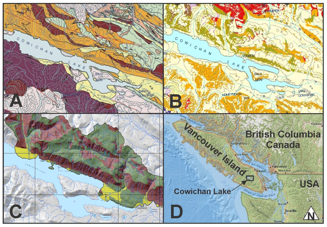
Figure 14 Cowichan Lake on Vancouver Island showing (a) bedrock geology and volcanics of the Sicker Group (orange), Bonanza Group (purple) and Karmutsen Formation (pink); (b) mass movement potential (0.004 $\mathrm{landslides}{\mathrm{km}}^{-\mathrm{2}}{\mathrm{yr}}^{-\mathrm{1}}$ for the orange zone, up to double that for the tan zone on the north side of the lake); (c) surficial geology (colluvium, till, and fluvial gravels mapped as purple, green, and yellow, respectively); and (d) the overall location. Figure taken from Guthrie (2005a) (a, b) and Palmer (2018) (c).

The lowest slopes in the Cowichan Lake valley, adjacent to the shore, are home to approximately 1700 people, and 240 homes were identified as occupying an extreme risk zone related to potential landslide runout (Ebbwater and Palmer, 2019). A landslide runout model was needed to differentiate modern debris flow runout zones from paraglacial fans and the floor of the U-shaped valley and better discretize risk.

3.2.2 Running the model

Modeled landslides were initiated using DebrisFlow Predictor in each of four preassigned zones representing a hazard, respectively, of 0.004, 0.001, 0.0005, and 0.00007 $\mathrm{landslides}{\mathrm{ha}}^{-\mathrm{1}}{\mathrm{yr}}^{-\mathrm{1}}$ (Palmer, 2018).

Landslide initiation locations were created by importing, within the zones described above, randomly distributed points, a uniform distribution of points, and manually chosen points using the GIS tool and lidar within DebrisFlow Predictor and experience in similar areas (Fig. 15). The results of each run were compared in a calibration exercise.

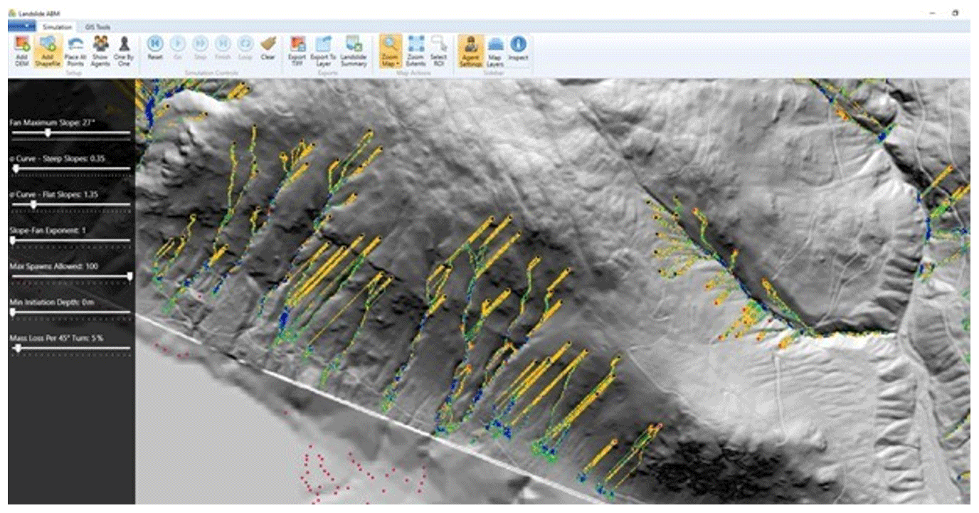
Figure 15 Test run of simulated landslides along the north shore of Lake Cowichan. Yellow represents scour, and green and blue represent deposition (blue is deeper).

There was no significant difference in outcomes between landslides generated using random, uniform, or manually chosen initiation points other than manually selected initiation zones were more likely to run successfully. Using the random or uniform distribution of initiation points meant that some agents were generated on local slopes too flat to initiate a landslide response. Manual selection simply reduced the probability that this would occur.

Magnitude–frequency analyses revealed some differences between mapped and modeled landslides (Fig. 16). The tangent of the slope at a given probability of occurrence was approximately equal for both modeled and mapped landslides, and we interpret that the model does a good job representing variability in landslide size distribution. However, mapped landslides generally occupied about twice the area of modeled landslides.

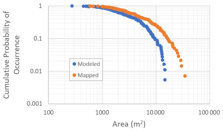
Figure 16 Magnitude–frequency comparison between modeled (blue) and mapped (orange) landslides on the north shore of Cowichan Lake, BC.

We explain this by observing that mapping is, in and of itself, a model that includes restrictions related to level of detail and a practical mapping scale. The mapper must make a choice between outlining landslides that are inferred to exist on steep slopes and precisely following the limited path visible among trees. In this case, the model appears to have better limited the landslide width to the actual path (Fig. 17). Mapped landslides include areas of steep gullies and slopes that are heavily forested after the identified event. We therefore interpret that the magnitudes of the mapped landslides are conservatively inflated and that is reflected in the curve in Fig. 16.

Despite differences in magnitude and frequency, modeled landslides traveled consistently further than mapped landslides. Fanning behavior modeled did approximate vegetation changes on the fan but exceeded what had been observed in the last several decades of air photograph interpretation.

3.2.3 Calculating landslide runout

Once tested, 1364 new landslide initiation points were selected across each of the four hazard zones. DebrisFlow Predictor then automatically created initiation zones (as a selected option) of nine agents in 15 m by 15 m grids (where grid cells are 5 m on each side; see Fig. 18).

A total of 50 landslide runs were modeled from each landslide initiation zone. Though viewable in DebrisFlow Predictor, the results were exported as GeoTIFFs to enable visualization in Google Earth and ArcGIS software (Fig. 19). Over 70 000 debris flows were modeled and a distinct runout limit was derived.

The result of the landslide runs was, with few exceptions, that the cumulative footprint of modeled landslides did not reach residential homes on the paraglacial fans. Instead, landslides tended to terminate on upper-fan and mid-fan slopes that were between 10 and 20^∘. Modeled landslides, as observed in the testing phase, traveled consistently further than mapped landslides.

The likelihood of any individual landslide reaching the runout limit was explored in DebrisFlow Predictor by obtaining information about the number of times any pixel was inundated out of the total number of runs. In this instance, however, the total runout limit was more practical (Fig. 20).

Table 5 Assigned debris flow damage classes.

3.2.4 Estimating likelihood of damage

The probability of damage due to debris flows and debris avalanches has been discussed by several authors and can be modeled empirically (Jakob et al., 2012; Papathoma-Kohle et al., 2012), analytically (Corominas et al., 2014; Mavrouli et al., 2014), or using engineering judgment (Winter et al., 2014). Ciurean et al. (2017) developed an analytical method that required only depth and compared favorably to both empirical and analytical methods previously developed.

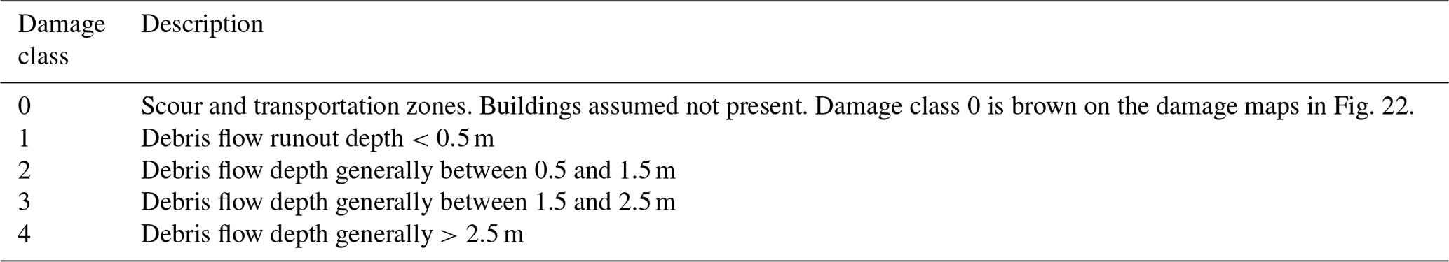
The latter method was used to estimate the potential impact of debris flows or debris avalanches that were modeled to reach buildings (Fig. 21). A damage class was assigned to each polygon based on estimated landslide depth from the DebrisFlow Predictor model (Table 5), and potential degree of loss was determined as shown in Fig. 22 for different classes of buildings.

3.2.5 Case II: summary

DebrisFlow Predictor was used to model debris flow runout from steep slopes above a community on the north shore of Cowichan Lake.

With few exceptions, the cumulative footprint of modeled landslides did not reach residential homes on the paraglacial fans.

Exceptions were easily identified on two types of maps: a runout limit map and a potential damage map that relates to building vulnerability.

With over 70 000 landslide runs, the probability that a modeled debris flow will exceed the distal limit indicated on the maps was less than 0.000015.

Properties above (north) of the distal limit of modeled runout can use the potential damage curves to inform subsequent investigation.

4 Discussion and limitations of use

All models are wrong, but some are useful. (George E. P. Box; Box and Draper, 1987)

Both case studies demonstrate the potential usefulness of an easily employed, regional runout model. DebrisFlow Predictor is predictive and, at least for shallow, rapid to extremely rapid, flow-type landslides, appears to provide viable runout results, as well as information about landslide depth, area (footprint), and volume.

However, DebrisFlow Predictor is still limited to the rules for erosion and deposition employed, and experiments in other regions of the world will benefit users.

Some of the potential pitfalls of the program are articulated below.

4.1 Depth variability

As an artifact of the rules, individual runs may exhibit sudden deposition or scour along their path in excess of what would actually be expected. This occurs when a single agent at a pixel picks a low probability depth for either scour or deposition. Multiple model runs are therefore recommended and should provide better depth results because individual highs and lows are averaged out. Depths should be field verified wherever possible.

4.2 Parameter sensitivity

There are considerable opportunities to tweak landslide behavior within the program. Runout depends on initial volume as well as the difference in available entrainment along the landslide path. The professional landslide specialist needs to consider these criteria and measure results against actual conditions when calibrating the model.

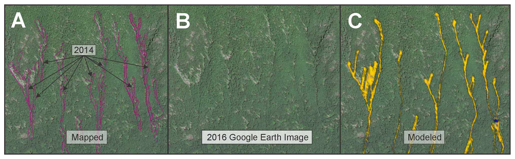
Figure 17 Mapped landslides from 2014 images (a) in the study area were typically wider than observed (b) or modeled landslides (c) in the study area and resulted in mapped magnitudes about twice that of modeled magnitudes for the same frequency of occurrence. Background image © Google Earth, 2016.

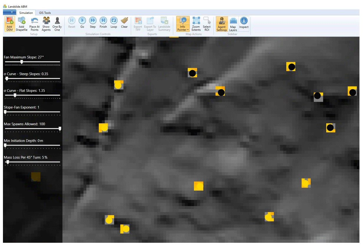
Figure 18 A close-up view of landslide initiation points and the DebrisFlow Predictor generated 15 m×15 m initiation zones. Each zone contains nine agents. The sliders on the left control agent behavior as explained in the Methods section.

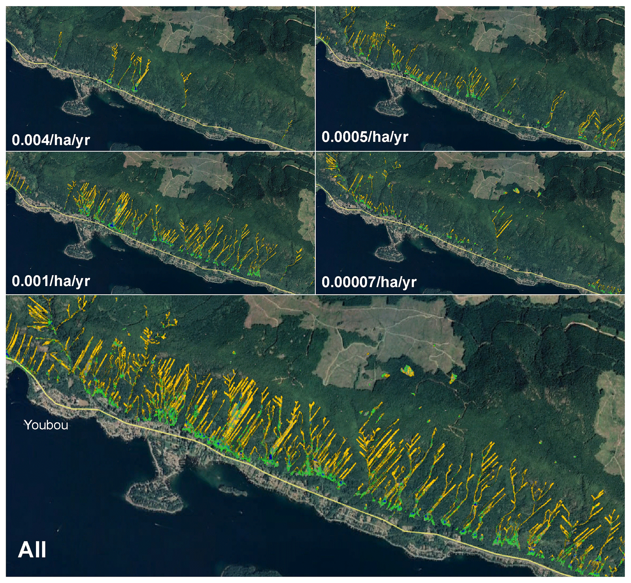
Figure 19 Modeled landslides along the north shore of Cowichan Lake from different hazard zones and overall. Results can be imported into Google Earth, as shown here, for convenient visualization (background image © Google Earth).

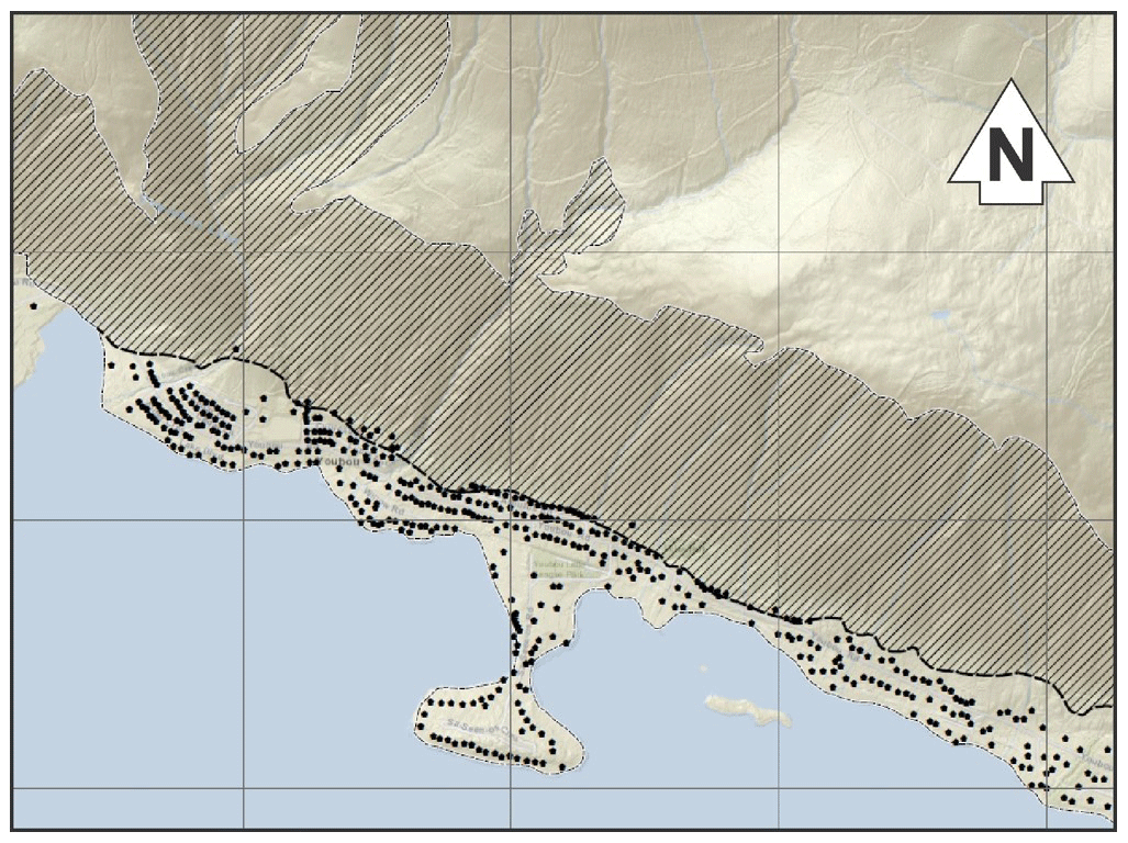
Figure 20 Modeled debris flow runout limit. Note that most of the 240 properties (black pentagons) are outside the modeled runout zone. Background image © ESRI World Topographic Map.

Figure 21 Vulnerability identified by degree of expected loss for constructed buildings by debris flow depth (Ciurean et al., 2017).

4.3 Linearity

Very steep slopes may produce a strong linear landslide orientation, which is easily seen when multiple landslides are triggered. This occurs when the DEM at the model resolution (5 m) is so steep that it overwhelms the path selection at each time step and spreading has not yet occurred (recall that spreading is has a user-defined slope limit). While natural analogs are readily found (e.g., Fig. 23), the modeled results may nonetheless bypass local topographic effects and choose paths that vary somewhat from the real-world equivalent. DEM effects have been noticed by others; Degetto et al. (2015) and Stolz and Huggel (2008) both demonstrate that the DEM source can dramatically influence the outcome of debris flow models, even at equivalent resolutions. Horton et al. (2013) propose that a 10 m resolution DEM is appropriate for regional mapping. In our case, we suggest that the 5 m DEM strikes the right balance between processing power and reasonable results, and DebrisFlow Predictor has been optimized such that the agents work on a 5 m cell size.

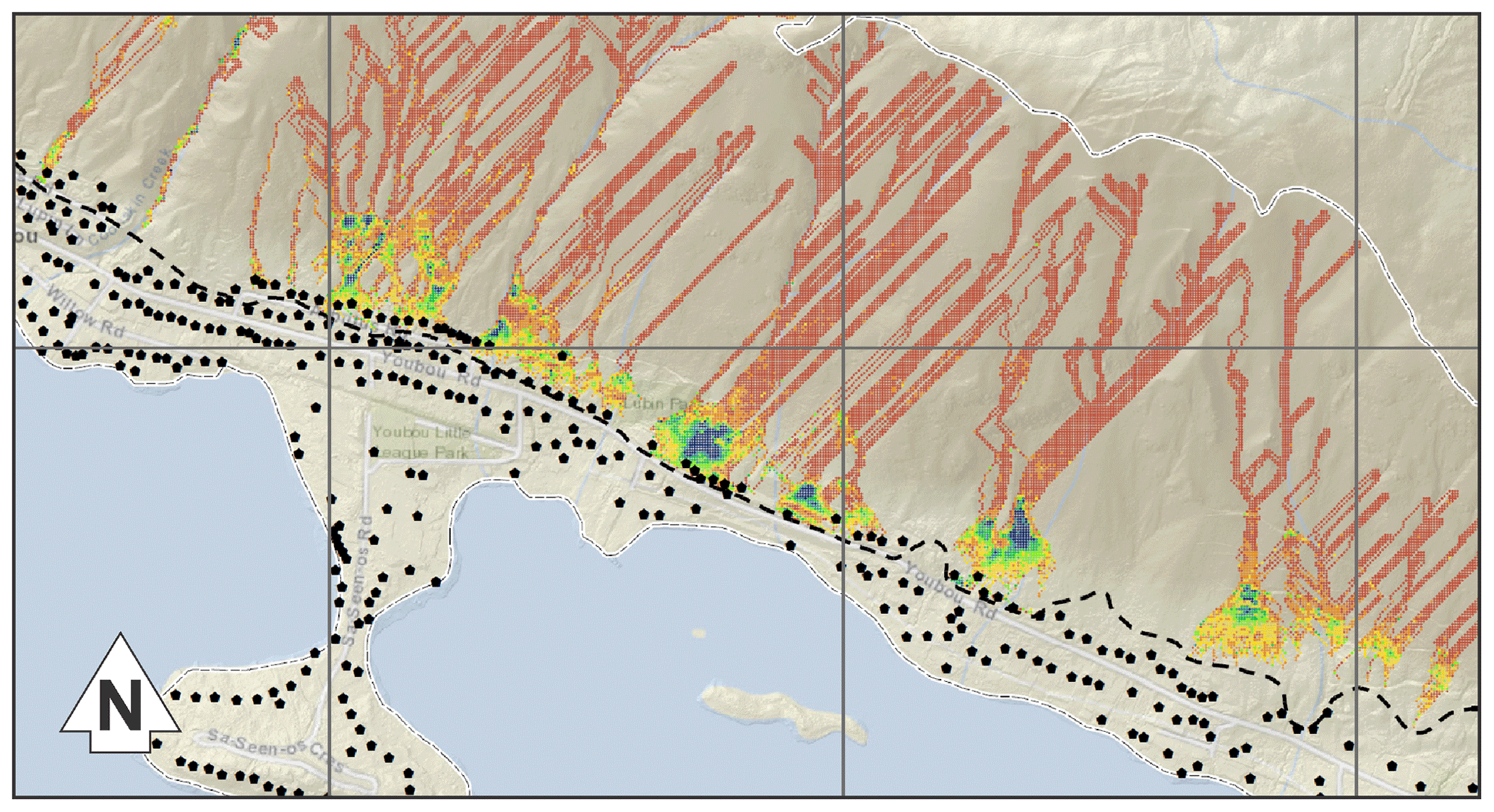
Figure 22 Damage map for the north shore of Cowichan Lake. The color classes match Fig. 21. The darker brown represents scour and transport zones and construction is assumed unlikely. Background image © ESRI World Topographic Map.

Figure 23 Strong linear orientation of landslide tracks on steep slopes in Indonesia (a) where multiple landslides occur at once and on the north shore of Cowichan Lake (b) where multiple landslides were modeled to occur at once (background images © Google Earth).

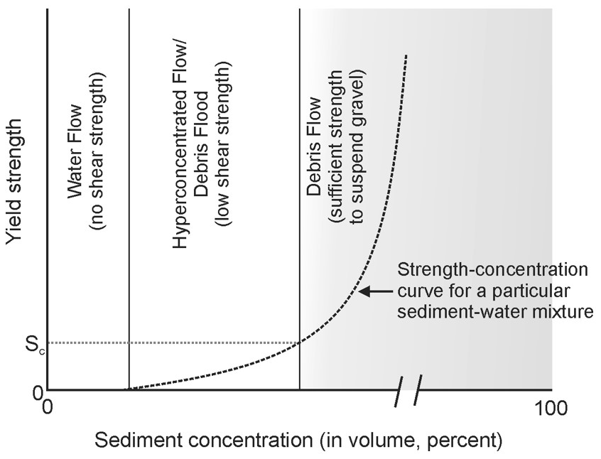
Figure 24 Debris flows as expected to be modeled by DebrisFlow Predictor (shaded area). S_C represents the critical shear strength beyond which gravel (4 mm or larger) is suspended. Figure is modified slightly from Pierson (2005).

4.4 Debris flows vs. debris floods

Despite considerable literature, confusion about the difference between debris flows, debris floods, and hyperconcentrated flows persists (Pierson, 2005; Calhoun and Clague, 2018; Keaton, 2019; Church and Jakob, 2020). Geomorphic criteria for distinguishing between debris flows and debris floods such as those derived by Wilford et al. (2004) may not fully align with other defining criteria such as sediment concentration and shear strength (Fig. 24).

DebrisFlow Predictor simulates rapid to extremely rapid landslides of the flow type but is not intended to model debris floods or hyperconcentrated flows. DebrisFlow Predictor may therefore underestimate runout of channelized debris flows particularly those channels that are transitional to debris floods. However, as demonstrated in our case study, DebrisFlow Predictor can provide volumetric sediment supply to channels that can be subsequently modeled using the right tool. Further, within its intended parameters (the empirical observations of scour and deposition), DebrisFlow Predictor tends to show the depositional extent of debris flows in channels that might be otherwise lost to other processes. Nonetheless, the process difference should be recognized by the reader.

4.5 Detailed simulation

DebrisFlow Predictor is a regional tool based primarily on empirical observations of aggregate debris flow behavior, particularly scour and deposition along the landslide path. Its probabilistic nature will result in similar but different outputs from one run to the next. We would expect nature to behave much the same way. However, if a detailed analysis of a single debris flow is sought, it does not address the site-specific controls such as rheology, topography finer than 5 m, moisture content, and geology (among other factors). Indeed, DebrisFlow Predictor explicitly seeks to ignore these factors in order to provide a practical regional tool. For a detailed analysis, the reader is directed to any of several excellent dynamic models.

5 Conclusions

In order to address a perceived need for a debris flow or debris avalanche runout model that can be applied regionally with relatively few inputs, we developed, and present herein, an agent-based landslide-simulation model called DebrisFlow Predictor. DebrisFlow Predictor is a fully predictive model whereby autonomous subroutines, or agents, act on an underlying DEM using a set of probabilistic rules for scour, deposition, path selection, and spreading behavior. Along the way, agents keep track of the changes they make to the DEM, the landslide to which they belong, nearby (adjacent) agents, and their own mass balance.

We demonstrate the use of DebrisFlow Predictor in two case studies.

In the first, we used DebrisFlow Predictor to determine the sediment input (in m³) to a stream network in the steep mountains of Indonesia's province of Papua. Sediment input was used to bulk the hydrographs for subsequent debris flood modeling (not shown) at specified return periods.

In the second case study, we used DebrisFlow Predictor to predict runout distance in a residential community on Vancouver Island, Canada. By running tens of thousands of landslides, we defined a modeled landslide runout limit and demonstrated that most houses were beyond the threat of debris flow runout. For those that remained in the runout zone, we used the average depth information to assign potential damage curves to unprotected properties.

DebrisFlow Predictor is freely available for non-commercial use (e.g., universities and research departments) and may be downloaded here: http://landing.stantec.com/debris-flow-predictor-download-request.html (last access: 16 March 2021).

DebrisFlow Predictor simplifies extremely complex behavior to provide reasonable predictions of outcomes. Should there be a perceived difference between modeled results, and on-the-ground evidence, the ground-based evidence should take priority. DebrisFlow Predictor does not relieve professionals from using their experience, training, and education to make good judgments when assessing actual ground conditions but provides additional understanding of processes and credible outcomes.