the Creative Commons Attribution 4.0 License.
the Creative Commons Attribution 4.0 License.
 | 14 Dec 2020
New global characterisation of landslide exposure
Robert Emberson
Dalia Kirschbaum
Thomas Stanley
Landslides triggered by intense rainfall are hazards that impact people and infrastructure across the world, but comprehensively quantifying exposure to these hazards remains challenging. Unlike earthquakes or flooding, which cover large areas, landslides occur only in highly susceptible parts of a landscape affected by intense rainfall, which may not intersect human settlement or infrastructure. Existing datasets of landslides around the world generally include only those reported to have caused impacts, leading to significant biases toward areas with higher reporting capacity, limiting our understanding of exposure to landslides in developing countries. In this study, we use an alternative approach to estimate exposure to landslides in a homogenous fashion. We have combined a global landslide hazard proxy derived from satellite data with open-source datasets on population, roads and infrastructure to consistently estimate exposure to rapid landslide hazards around the globe. These exposure models compare favourably with existing datasets of rainfall-triggered landslide fatalities, while filling in major gaps in inventory-based estimates in parts of the world with lower reporting capacity. Our findings provide a global estimate of exposure to landslides from 2001 to 2019 that we suggest may be useful to disaster mitigation professionals.
- Article
(7932 KB) - Full-text XML
-
Supplement
(780 KB) - BibTeX
- EndNote


Rainfall-induced rapid landslides are an important natural hazard in many countries around the world, both as independent events and within larger chains of cascading hazards due to their role in downstream debris flow hazards. Current estimates of landslide impacts suggest that they cause thousands of fatalities annually (Froude and Petley, 2018; Petley, 2012) and billions of dollars of economic damage (Dilley et al., 2005). Global hazard estimates are an important way to understand the relative efficacy of hazard mitigation mechanisms between different countries, and they also provide policymakers with tools to estimate the future challenges associated with landslide hazards. However, few studies exist at present that provide a globally consistent set of estimates for landslide hazard, and even fewer that attempt to characterise risk and exposure.
Most studies of landslide impacts rely on observations of specific landslide events and the associated reporting of the impacts. A small number of studies have estimated global economic impacts (Dilley et al., 2005; Guha-Sapir and CRED, 2019), while other important work has collated the fatalities associated with landsliding around the world to give crucial insight into impacts (Froude and Petley, 2018; Petley, 2012). The reliance of these studies on landslide inventories leaves them subject to known biases associated with these inventories. Specifically, there tends to be better reporting in developed countries (Kirschbaum et al., 2010; Monsieurs et al., 2018) and a lack of public data about landslide occurrence and impacts in more remote regions, resulting in major blind spots in Africa, portions of the Andes, western China, and parts of Indonesia and the Philippines.
The global coverage of satellite data offers opportunities to fill in data gaps that result from inventory-based assessment of landslide hazards. NASA's Landslide Hazard Assessment for Situational Awareness (LHASA) model provides an estimate of landslide hazard between 50∘ N and 50∘ S, at 30 arcsec resolution, based on a global susceptibility map and inputs from NASA precipitation estimates (Kirschbaum and Stanley, 2018). This is updated every 3 h, with a latency of approximately 4 h, providing a near-real-time output. Using this model, it is possible to estimate relative changes in landslide hazard around the world each year. More importantly, this approach does not rely on local inventories to characterise the hazard and therefore provides a near-global, consistent estimate of landslide hazard, encompassing the vast majority of populated areas. To address the need for globally consistent data on landslide hazard and exposure, we utilise an updated and enhanced version of the global susceptibility model defined by Stanley and Kirschbaum (2017) combined with a newly available 19-year IMERG rainfall product (Huffman et al., 2018) to estimate global landslide hazard, and then combine this with global estimates of population and critical infrastructure.
This information can also be considered together with other datasets such as Froude and Petley (2018) to assess relative vulnerability to landslide exposure in different countries. A globally consistent model could support hazard mitigation decision-making and planning, particularly in developing countries with limited reporting capacity. Our exposure model outputs derived from the LHASA model provide an estimate of exposure seasonality at 30 arcsec resolution across the globe. This demonstrates the value of using remote sensing data in concert with ground-based inventories to provide a more spatially consistent picture of the impacts associated with landslides around the world. While the model outputs are an approximation of exposure to hazard based on historical rainfall trends, we note that future exposure patterns could be explored with the use of rainfall projections for future climate scenarios.
To estimate exposure to landslide hazard, we must first derive the estimates of hazard itself. For this study, we have utilised the outputs of an updated version of the LHASA model as an approximation for hazard, which we can then combine with openly available datasets of infrastructure at a 30 arcsec resolution across the world. These maps of exposure, both annually and estimated for each month to analyse seasonal variability, are an important initial output in their own right, but we have further analysed the data to compare our outputs with existing estimates of global landslide hazard. This provides key insights into where existing inventory biases may exist, as well as highlighting which countries and regions are most exposed to rainfall-triggered landslide hazard. Below, we detail the methods used to generate these outputs.
2.1 Hazard estimates derived from the LHASA model
The LHASA model is designed to provide near-real-time awareness of potential rapid landslide activity through landslide “nowcasts” (Kirschbaum and Stanley, 2018). The algorithm uses a susceptibility map calculated from globally available estimates of slope, lithology, forest cover change, distance to fault zones and distance to road networks to provide a relative estimate of static susceptibility (Stanley and Kirschbaum, 2017). This susceptibility is divided into categories based on decreasing area of the world occupied by each increasing class: this classification scheme was designed so that each category was twice as large as the next highest; for example, the very low category contains roughly twice as many pixels as the low category. The susceptibility map is then compared with satellite-based precipitation estimates from NASA's Tropical Rainfall Measuring Mission (TRMM) Multi-satellite Precipitation Analysis (TMPA) and Global Precipitation Measurement (GPM) Integrated Multi-satellitE Retrievals for GPM (IMERG) rainfall product. To characterise the potential for landslide triggering, an antecedent rainfall index (ARI), or weighted accumulation from the last 7 d of rainfall, is calculated at each pixel. The weighting is an exponential weighting, with each day prior to the most recent multiplied by 1∕n2, where n is the number of days prior to present. The exponent value of 2 was calculated by Kirschbaum and Stanley (2018) based on calibration at the locations of 949 landslides from the years 2007–2013.
If the ARI value exceeds a threshold (historical 95th percentile for rainfall), either a moderate-hazard or a high-hazard nowcast may be generated if there is moderate to high susceptibility within that area. Nowcasts are issued at a 30 arcsec (approximately 1 km at the Equator) pixel resolution every 3 h. For the purposes of our study, we use the daily nowcast output, which is generated based on daily rainfall totals rather than 3 h totals. The physical meaning of one nowcast is 24 h of elevated landslide hazard for a 30 arcsec dimension pixel.
We have updated the LHASA model for this study to incorporate data made available since the initial version of the model. We term this revised model “LHASA 1.1”. First, the global landslide susceptibility map (Stanley and Kirschbaum, 2017) was updated to include the 2018 data on forest loss since the year 2000 (Hansen et al., 2013) and road density from the Global Roads Inventory Project (GRIP; Meijer et al., 2018). Previously, the forest loss data were modelled as a binary variable representing either the presence or absence of any 30 m forest loss pixel within each 30 arcsec grid cell. However, this update represents forest loss at 30 arcsec as a fraction of the 30 m grid cells which have recently experienced forest loss (from 2000 to present). The effect of this change will be to de-emphasise the role of forest loss at locations with little recent disturbance, but not to change the effect of forest loss on any 30 arcsec grid cell which has experienced total loss of all forest cover. The susceptibility map was recomputed at 30 arcsec resolution using the same fuzzy overlay methodology as the previous version. This fuzzy overlay model uses heuristic weighting of the input variables, defined by Stanley and Kirschbaum (2017). We do not adjust the weights attached to the variables in the study here. We assess the accuracy of the new susceptibility map in the same fashion as in the study of Stanley and Kirschbaum (2017), by using the NASA Global Landslide Catalog (GLC) locations to test the ROC-AUC (receiver operating characteristic and area under the curve) values. Using the same GLC data that were used to calibrate the previously published version of the susceptibility model (GLC data snapshot of 14 January 2016), we calculate an ROC-AUC value of 0.822, essentially identical to the value obtained for the prior model (0.82). For the purposes of our analysis, we follow Stanley and Kirschbaum (2017) and divide susceptibility into multiple classes, and use the threshold between “low” and “moderate” susceptibility as a threshold for nowcasts to be generated if rainfall exceeds the historical 95th percentile. Less than 25 % of landslides recorded in the GLC occur below this threshold. For the purposes of this study, we combine moderate and high nowcasts together to provide a proxy for hazard that captures the bulk of landslide activity.
Secondly, we have updated the rainfall input. Due to a recently released near-20-year record of IMERG (version 6B), we have modified the precipitation inputs to LHASA in the following ways. First, we extend the LHASA model from 50∘ N–S, which was the latitudinal extent of TMPA, to the 60 ∘ N–S extent of the IMERG product (Huffman et al., 2018). This latitudinal expansion now includes most of northern Europe and Canada, and the only populated areas excluded are in northern Russia, Iceland, some of Scandinavia and Canada. Because falling snow is an important component of precipitation at higher latitudes but not a major trigger of landslides, we changed the precipitation variable considered from total precipitation to just rainfall. The LHASA model does not consider snow avalanches. The effects of this change should be minimal in the tropical and temperate zones previously studied.
The LHASA model generates a hazard nowcast if rainfall exceeds the historical 95th percentile and susceptibility exceeds the “moderate-susceptibility” threshold. Since the updated model uses IMERG v06B rather than TMPA, we have therefore re-calculated the historical 95th percentiles of a 7 d weighted rainfall accumulation (based on 2000–present IMERG rainfall data). This provides a global 95th-percentile map; if ARI values exceed this threshold, a hazard nowcast is issued. The model is then reprocessed from 2000 to present, and we build a 19-year record of landslide nowcasts around the world. Averaging the nowcasts by month, we construct a nowcast climatology, or average landslide nowcast rate for each pixel. We also compute annual nowcast rates. This provides a globally consistent proxy for landslide hazard over the course of the year at each location. We term this as “nowcast density”, and it represents a proxy for intensity of landslide activity. We can then combine this with data on population and infrastructure to assess the relative exposure to landslides.
The result is a raster dataset at 30 arcsec resolution for each month of the years in the IMERG record. We compute additional metrics such as the inter-annual variability in nowcast frequency and standard deviations of nowcast frequency. This information is incorporated into the annual exposure estimates to provide a measure of the variability. This uncertainty analysis is discussed in more detail below.
2.2 Exposure datasets and integration with hazard
We have overlaid the hazard footprints derived from the LHASA-based nowcast climatology on top of publicly available datasets of population and infrastructure globally to map the exposure of these elements to landslide hazard. We have additionally aggregated these data at a national scale to compare with existing studies. Below, we first describe the datasets used and then describe the approach taken to combine them with the hazard outputs.
We use population data from the Gridded Population of the World version 4 dataset (Doxsey-Whitfield et al., 2015), adjusted to the UN WPP Population Density for 2015. Use of this dataset is in line with other studies of population exposure to global hazards (Carrao et al., 2016; Dilley et al., 2005; Kleinen and Petschel-Held, 2007). The resolution of this dataset is the same as the LHASA nowcast output – 30 arcsec – and thus can be directly mapped onto the hazard data.
The definition of critical infrastructure can differ depending on the relevant stakeholder or location. The UN Global Assessment Report 2015 incorporates schools, hospitals and residential areas (De Bono and Chatenoux, 2014), and we use this as an initial basis for our estimates. We incorporate roads as defined in GRIP (Meijer et al., 2018), and amenities including hospitals, schools, fuel stations and power facilities as defined by OpenStreetMap (OSM). Both catalogues have a global extent and are updated regularly. Additionally, they offer a consistent set of data that can be compared across the world. While there are some caveats to this comparison, which are discussed below, we suggest that these two datasets are likely the best datasets with global coverage, open access and recent updates.
The GRIP roads dataset harmonises nearly 60 datasets describing road infrastructure into a single, consistent dataset covering 222 countries (Meijer et al., 2018). GRIP incorporates roads derived from OSM as well as other data sources and is considered to be a harmonised global road catalogue. The daily updates for OSM are not incorporated into GRIP, but we consider the globally harmonised nature to be more important than a frequently updated catalogue for the purposes of our study. This dataset is a shapefile of linear features, which is not initially directly compatible with the 30 arcsec resolution landslide hazard outputs. To connect the linear road dataset with the pixel-based nowcast-based landslide hazard data, we have used the Line Density tool in ArcGIS to calculate the density of roads at 30 arcsec resolution with an output of a road density map with units of kilometre per square pixel. Although the GRIP database classifies roads in one of five classes depending on size and importance (e.g. primary highway or residential road), we have not distinguished between these classes in our analysis. This dataset does not include footpaths or unpaved roads, for which mapping may be significantly more spatially inconsistent. While economic impacts vary based on the type of road, our analysis is meant to highlight the total potential exposed length for all types of roads.
OSM is a continually updated global map of infrastructure, roads, settlement and land uses (OpenStreetMap contributors, 2015). The updates are contributed by members of the public, and the data are openly available for access in shapefile and XML format. While differing levels of input from different parts of the world mean that there can be differences in the level of completeness of the map depending on the region (Barrington-Leigh and Millard-Ball, 2017), the specificity of the data makes it an excellent source for infrastructure information. There is detailed classification of different features in the map that allow us to isolate specific types of infrastructure, such as medical amenities or power stations. In addition, the open-source nature of OSM means this approach is highly replicable. We have used the Planet OSM data file (a single XML document of approximately 1 TB, containing the information for every mapped feature in the OSM map) and parsed the XML data using a Python-based script to obtain the density of critical amenities at a 30 arcsec resolution. We define critical amenities as those labelled “school”, “hospital”, “fuel station”, “power station” and other “power” nodes (including substations and transformers), based on the OSM feature definitions. We count each node as a single point, providing a density estimate of “nodes (school, hospital etc.) per 30 arcsec ×30 arcsec cell”, where nodes are of the types defined. The Planet OSM file was downloaded on 24 June 2019. The script used to parse this file is available in the Supplement.
To combine the roads datasets and OSM-derived critical infrastructure with the hazard outputs, we have multiplied the raster map of infrastructure or road density by the nowcast density raster (i.e. raster showing total days exposed to landslide hazard) for each full year in the IMERG archive (2000–2018) and taken the mean value and standard deviation. The resulting datasets on exposure for population, roads and critical infrastructure are all calculated at 30 arcsec resolution. We have also generated month-by-month exposure rasters to estimate the climatology of exposure for the same exposed elements. Since these outputs are based upon the LHASA nowcast output, it is important to clarify the units in which our estimates of exposure are expressed. Table 1 provides a summary of the units and the terms used in the study.
Table 1Summary of terms used to describe infrastructure and associated units.
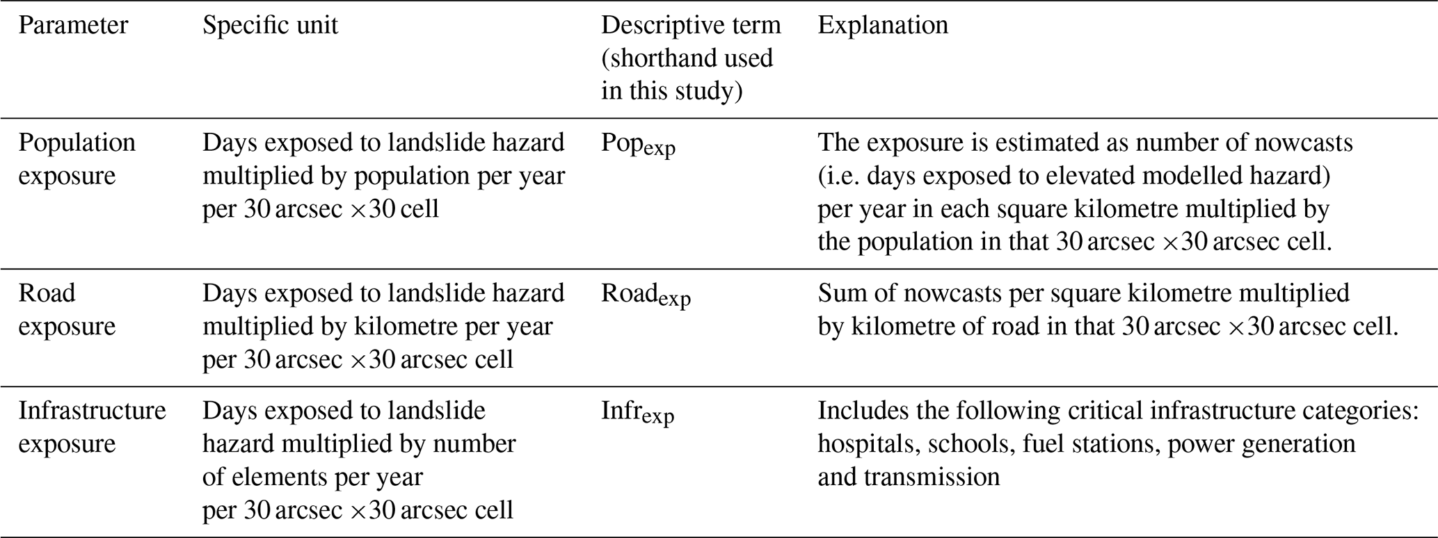
In Table 1, the units for each of the exposure outputs are also explained. We use the shorthand Popexp, Roadexp and Infrexp to denote population, road and infrastructure exposure respectively.
2.3 Error assessment
Kirschbaum and Stanley (2018) assess errors in the LHASA 1.0 nowcast hazard estimates by comparison with historical landslide events recorded in both the NASA Global Landslide Catalog (Kirschbaum et al., 2010) and the dataset of fatal landslides generated by Petley et al. (2007). They find relatively low false-positive rates (∼1 %) and moderate to good true-positive rates (24–60 % for moderate-hazard nowcasts). However, both the Global Landslide Catalog and the data of Petley et al. (2007) are not complete, meaning that the true- and false-negative rates are not easily quantified. More succinctly, since a complete dataset of landslide occurrence does not exist, it is challenging to calculate the accuracy associated with any independent landslide hazard estimate. Quantifying the relationship between nowcast density and landslide probability for a given area remains an important step for future research, and it requires spatially complete landslide catalogues with high temporal revisit rates. To explore the relative variability in landslide activity, we estimate the standard deviation in annual nowcast density at each point, based on the 19-year IMERG rainfall input. We then propagate the error into the estimates of exposure for population, roads and critical infrastructure. The raster data for the standard deviations in error are available in the supplemental data.
Estimating errors associated with OpenStreetMap data can be challenging, since the data quality is determined by volunteers who contribute to the map database. Broadly, we suggest it is appropriate to consider two distinct sources of error: the location accuracy of the individual points and infrastructure, and the completeness of the inventory. As discussed by Mooney et al. (2010), a lack of ground data across the world makes it challenging to assess the positional accuracy. However, at some locations, data can be compared with existing sources. In the UK, Haklay (2010) suggests that OSM data points offer positional accuracy comparable with the Ordnance Survey Maps (the government standard). For the purposes of our study, where the maximum resolution available for the landslide hazard data is 30 arcsec, this positional accuracy is in excess of the requirements. However, completeness of the map is more problematic.
Barrington-Leigh and Millard-Ball (2017) assess the relative completeness of the OSM roads data on a country-by-country basis, finding that OSM data in many developed countries are near complete, although this declines in some states with lower GDP. The completeness varies within individual countries, with the most complete mapping observed in the highest-density cities as well as the most sparsely populated areas (reaching a low in moderately populated areas). We assume that the estimate of completeness presented by Barrington-Leigh and Millard Ball (2017) for roads is applicable to other infrastructure; we are not aware of other global estimates of OSM completeness for specific infrastructure categories, so while this assumption may not fully hold we suggest it is more informative to use this completeness estimate than none at all. Note that this also assumes completeness is consistent within individual countries. The OSM completeness estimates are calculated at a national level, and it is therefore not clear how to apply them to the 30 arcsec pixels in our study. Thus we do not attempt to correct our global maps. However, to effectively normalise the exposure data at a country level, we provide the completeness measure derived from Barrington-Leigh and Millard-Ball (2017) in Table S1 in the Supplement. In the figures in the Supplement that show Infrexp aggregated at a national level, we normalise the exposed elements by the total number of critical infrastructure elements in each country, which serves to provide a useful inter-comparison of the relative hazard and does not require completeness metrics.
The GRIP roads database (Meijer et al., 2018) draws a significant part of the road inventory from OpenStreetMap and so is subject to some of the same error constraints. In Europe, the roads are derived primarily from OSM, although completeness in this part of the world is near perfect (Barrington-Leigh and Millard-Ball, 2017). GRIP also uses OSM data in China, where there is a dearth of other freely available datasets. As such, completeness estimates in China are difficult to accurately characterise, and we do not attempt to do so. Elsewhere, GRIP incorporates other road datasets to supplement OSM. These input datasets are limited to those with positional accuracy greater than 500 m, which precludes significant positional errors that would affect our kilometre-scale analysis. We are not aware of estimates of the completeness of the GRIP dataset; since it integrates datasets from all over the world, external validation datasets of completeness are unlikely to exist comprehensively. As such, while we note that there may be parts of the world where coverage is incomplete, we do not have strong constraints on this.
The results of our analyses provide a global set of model estimates of landslide exposure, both in raster format and tabulated by country. The source data are available in the Supplement associated with this study.
Figure 1 shows the modelled estimates of population exposure annually for each 30 arcsec pixel, and Fig. 2 shows the exposure of population, roads and critical infrastructure at the same scale for a portion of northern Italy and the Alps, to highlight the nature of the different datasets. As can be observed in Fig. 2, population and roads are significantly more widely distributed than critical infrastructure. Infrastructure is instead concentrated primarily in urban centres, although power distribution infrastructure follows similar transportation corridors to road networks. In other parts of the world, there are significant levels of exposure of critical infrastructure to landslide hazard. The co-location of power distribution and road network exposure highlights the potential for complex post-landslide damage and multi-sector impacts.

Figure 1Global modelled population exposure to landslides (Popexp). Since the distribution of high-exposure areas is highly localised, we have binned the data to highlight differences at lower exposure levels more clearly. The source for the country boundaries is UIA World Countries Boundaries, ArcGIS Hub, https://hub.arcgis.com/datasets/ (last access: 16 August 2019).
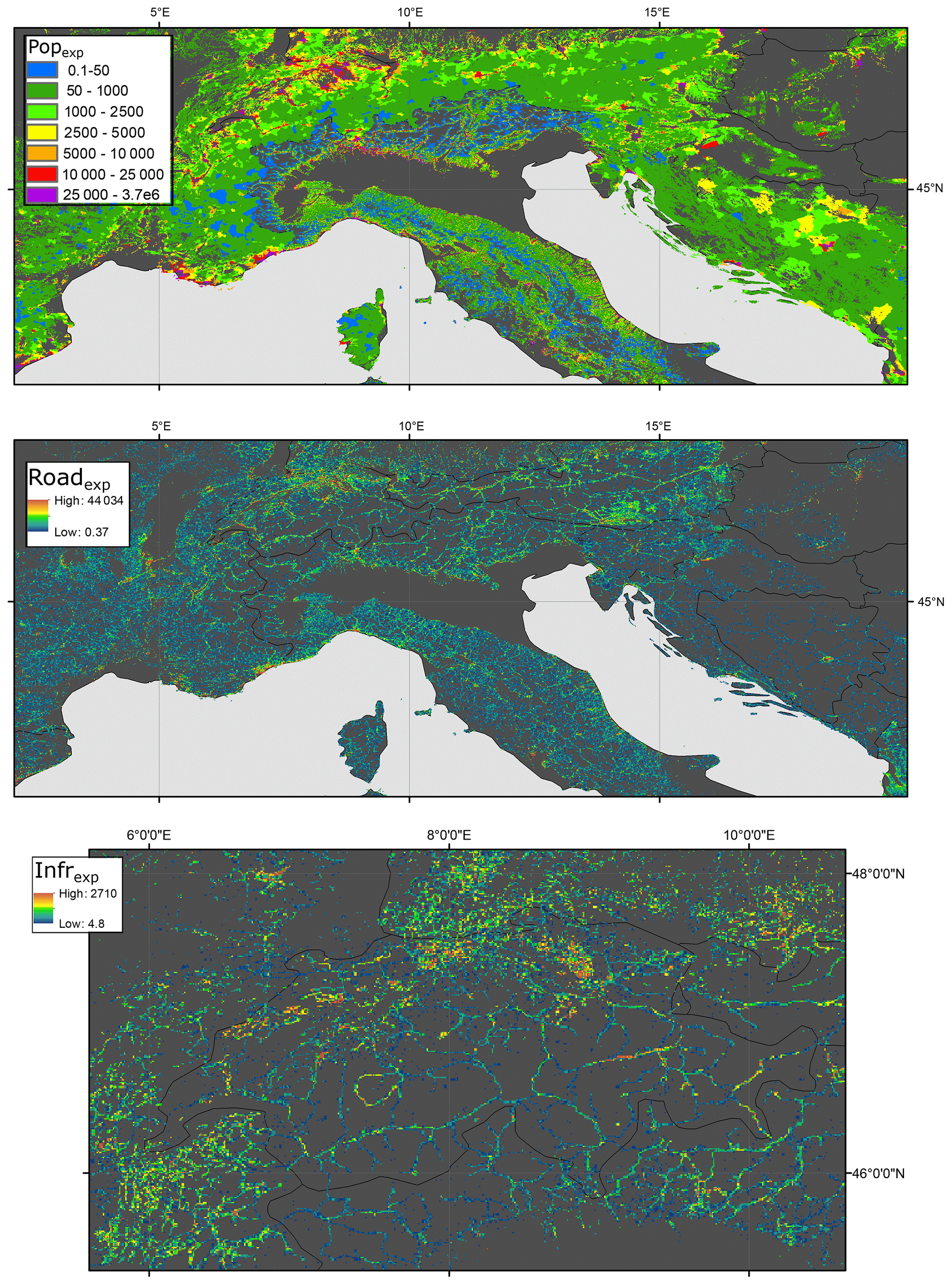
Figure 2Showing relative exposure of population, critical infrastructure and roads in a snapshot of the world map – in this case, the European Alps and Italy. To improve clarity, the critical infrastructure exposure is shown only for Switzerland.
For each country we have tabulated the aggregated values for Popexp, Roadexp and Infrexp, as well as average annual nowcast density. We also show the total population, total length of roads from GRIP and total number of OSM critical infrastructure elements; this allows for calculation of the fraction of the total that are exposed for each of these aspects. To normalise the number of nowcasts for each country, we divide by area in square decimal degrees, rather than square kilometers, since the nowcast data are output on a grid based on decimal degrees. The same aggregation approach could similarly be used at a sub-national level to assess relative impacts in different administrative areas. These data can be found in Table S1, where all data necessary to replicate these results are available.
Figure 3 plots the absolute numbers for Popexp, as well as the relative fraction of the population impacted by landslides. The relatively lower values in some of the larger countries like the United States and Brazil suggest that, while the overall population impact is high in highly populated states, the relative impact can be more concentrated in smaller countries.
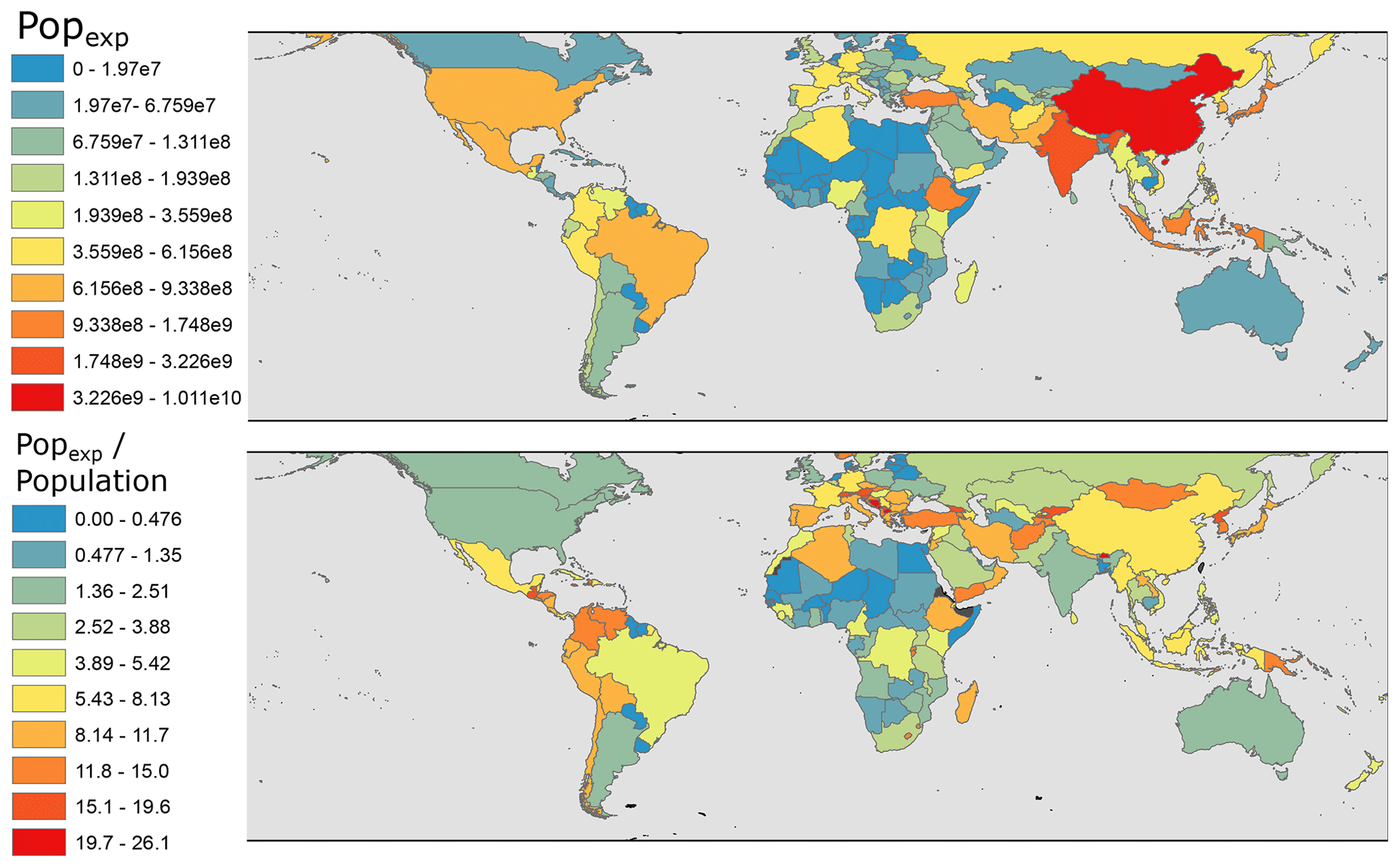
Figure 3Above: country-wide estimates of population exposure (Popexp). Below: population exposure normalised by total population. This is expressed as Popexp divided by total 2018 population derived from the World Bank data archives (World Bank, 2018). Countries in black in lower figure lack World Bank population estimates.
We also list the OSM completeness estimates from Barrington-Leigh and Millard-Ball (2017), the fatalities per country due to non-seismic landslides assessed by Froude and Petley (2018) and the landslide-linked economic impacts assessed by Dilley et al. (2005). These datasets are, to our knowledge, the most current datasets that assess landslide impact in terms of economic cost and fatalities globally, and they provide valuable points of comparison for our results.
The most striking initial result of our study is that significantly larger proportions of the globe are exposed to rainfall-triggered landslide hazards than are often considered (Fig. 1). Inventory-based assessments (e.g. Dilley et al., 2005) do not show significant levels of landslide hazard and exposure in sub-Saharan Africa or much of Asia and South America, while we find that many of these countries have significant proportions of the population and infrastructure exposed. It is perhaps not surprising that exposure to landslide hazard is elevated in the major mountain belts of the Andes and the Alpine–Himalayan orogeny, but there are other key hotspots that may be less well known. These areas include much of Japan, the Rwenzori Mountains in Africa, Central America and Mexico, and much of the Caribbean. We find specific hotspots for certain cities within or near mountain belts; this is particularly evident at the edges of large conurbations that abut mountainous areas, such as Taipei, Rio de Janeiro and the edges of Tokyo.
While the zones of densely packed critical infrastructure such as schools and hospitals are also in general associated with these urban areas, the exposure of linear infrastructure to landslides is more widespread. Roads and power transmission facilities often follow similar linear corridors, and where those intersect areas of high landslide hazard the relative exposure can still be important. The localised impact of a single landslide impacting a densely populated urban zone may be very high, with several critical infrastructural elements impacted. However, the likelihood of a landslide occurring somewhere along lengthy road or power transmission segments in regional-scale rainfall events is higher, and an interruption to linear infrastructure may impact lifelines that are relevant in disaster response. Thus the localised and distributed impacts should be considered alongside one another. We suggest that highlighting the most vulnerable corridors for power transmission and road traffic is an important subject for future work.
To explore these results against independent datasets of landslide hazard and risk, we have aggregated the data at a country level (Table S1). We can then highlight those nations with the highest landslide impact both in absolute terms (total exposed people and infrastructure) and as a proportion of the overall population or infrastructure in that country.
As might be expected, without normalising for area, countries with the largest population have the highest overall modelled population exposure, although exposure in China exceeds that of India despite similar current population totals. Exposure of roads is also greatest in China and the United States, which are both highly populated with good OSM coverage. These absolute values are important, but we suggest that more insight can be gained by assessing the relative exposure of population and infrastructure in each country, as well as by comparing the different relative values between nations.
Inter-comparison of different countries can highlight those nations where the impact of landslides is greatest and can draw attention to smaller, less developed nations where landslide statistics from report-based inventories may be lacking.
Figure 4 plots Popexp against the mean nowcast density in that country, with colours denoting the geographic region. Results indicate that hazard and exposure are generally well correlated across different countries; similar relationships exist for both road exposure and critical infrastructure (see the Supplement for figures). At the highest end of this scale – i.e. those with high x-axis values – are smaller countries where mountainous terrain makes up much if not all of the area: Monaco; Bhutan; Andorra; and several Caribbean States: St Vincent and the Grenadines, Dominica, Grenada and St Lucia. In terms of population exposure, many countries in Asia and Africa have higher population exposure for an equivalent level of nowcast density when compared to European and some Central American countries. This results from the generally higher population of these states.
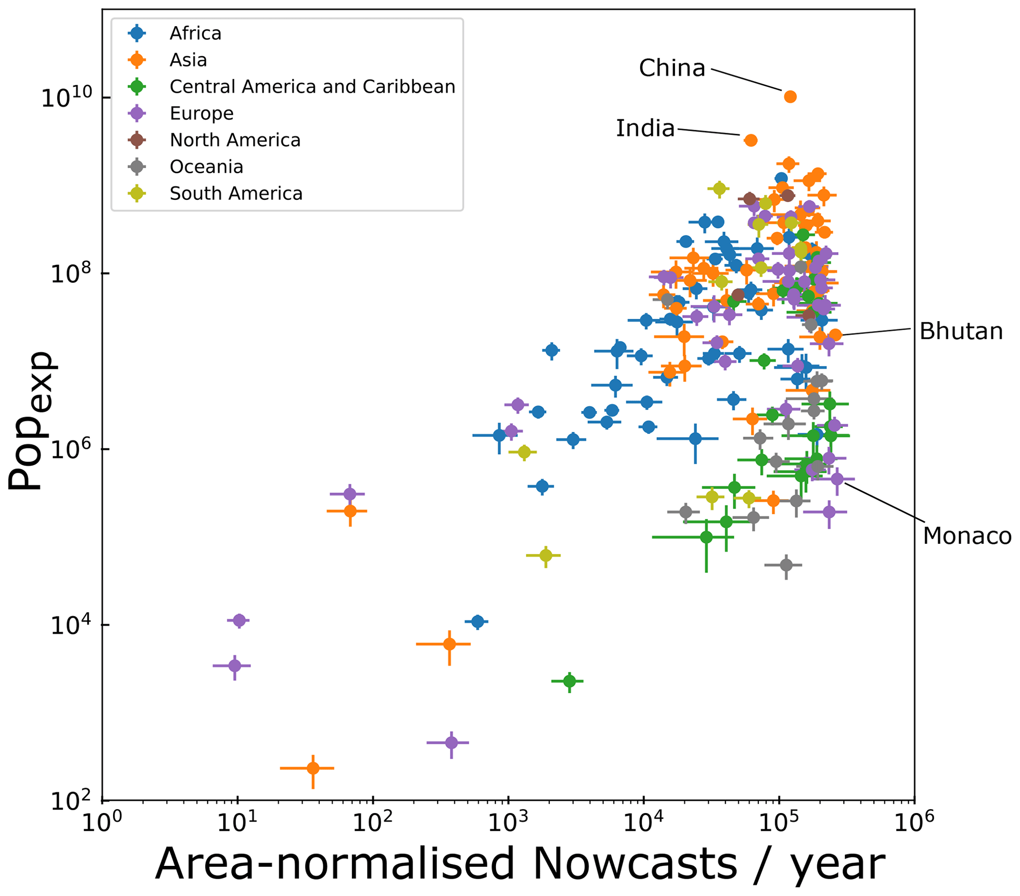
Figure 4Nowcasts per year, normalised by country area compared with the population exposed to nowcasts (in units of total days exposed to nowcasts multiplied by population per year).
Given the large degree of variability in annual nowcast frequency, inventories of reported landslides may misrepresent the average landslide rate in smaller countries if catastrophic landslides do not coincide with the sampling period for the inventory. At the same time, the LHASA-based model outputs are relatively insensitive to extreme rainfall events (100-year return period, for example), since all rainfall values above the 95th historical percentile will lead to the same nowcast hazard output. The bulk of reported landslide events occur in larger nations where statistical variability of landsliding is likely damped over larger areas like Nepal, Taiwan, China and Japan. While we find high normalised hazard estimates in many of those states, our analysis also highlights smaller nations where the relative impact of landslides may be more significant on longer timescales. Alongside the previously mentioned nations, we also find several smaller states with higher proportions of exposed population; Montenegro, Bosnia and Herzegovina, and Macedonia are notable in the Balkan area in particular.
To test whether the nowcast-exposure estimates are a useful predictor of landslide risk, we can compare them to existing datasets. In Fig. 5, we plot the total exposure of population in each country (in units of total days exposed to nowcasts multiplied by population per year) against the landslide fatality dataset assembled by Froude and Petley (2018). This dataset, collected from 2004 to 2016, consists of 4862 separate landslide events that resulted in fatalities and is the most comprehensive dataset for landslides that have caused fatalities in the world. Figure 5 highlights that there is a relatively strong correlation, with countries in Asia, Central America and Africa generally exhibiting higher numbers of fatalities for a given population exposure than observations in Europe.
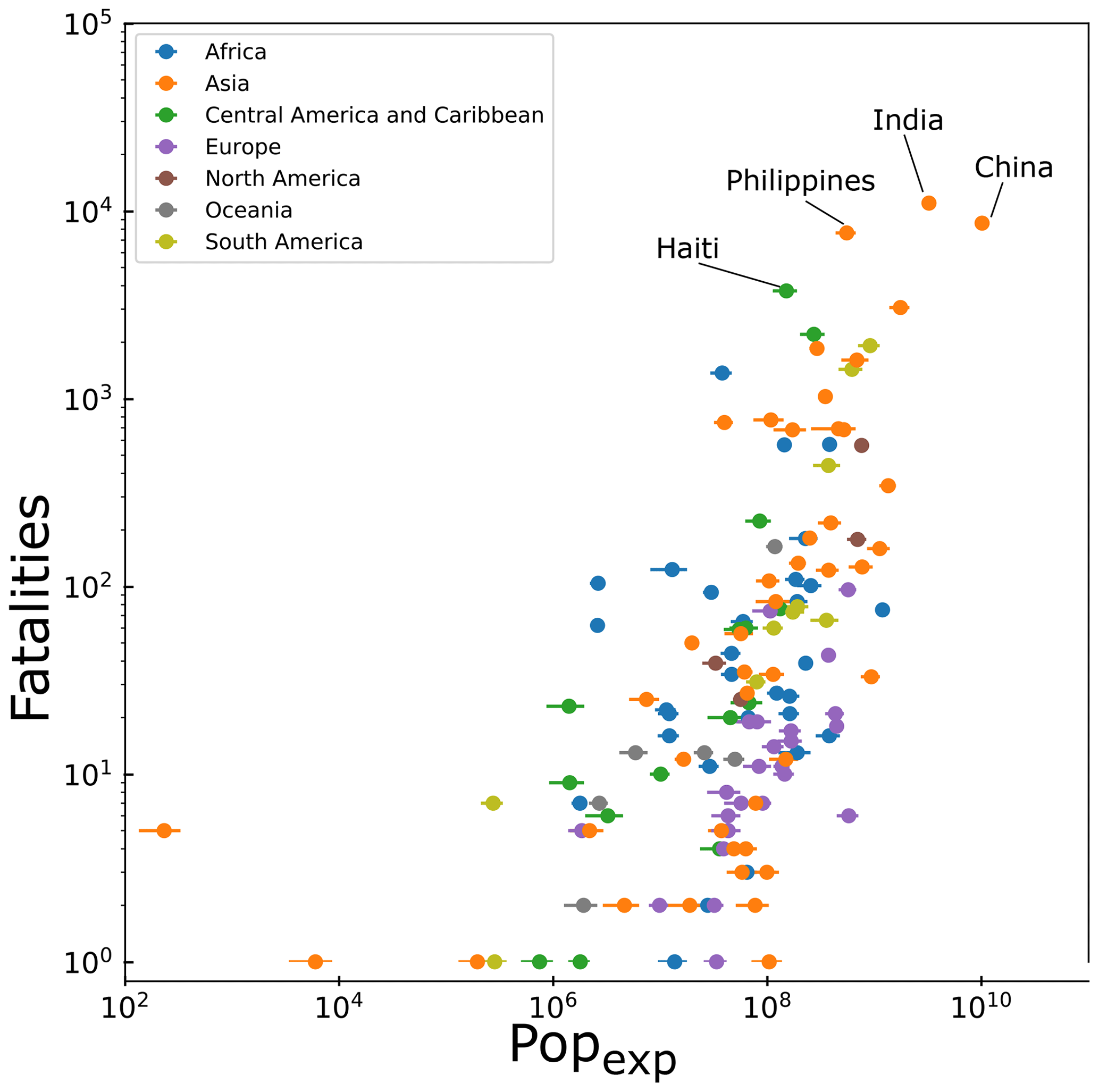
Figure 5Showing the exposure of population (in units of total days exposed to nowcasts multiplied by population per year) against the number of total fatalities recorded in the dataset of Froude and Petley (2018).
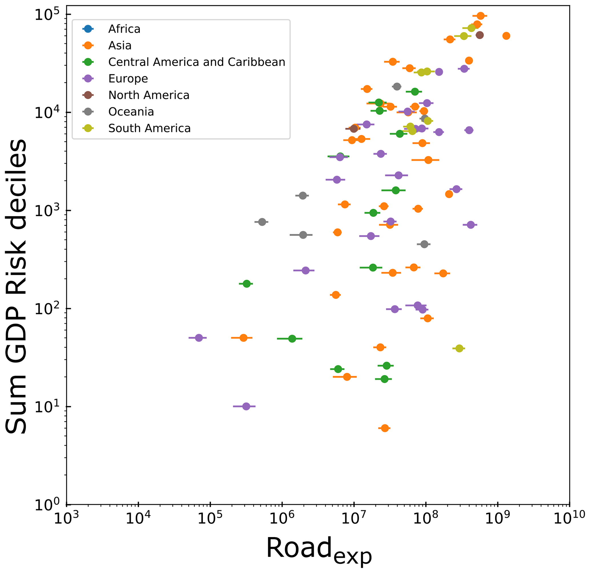
Figure 6Plotting the exposure of roads (in units of sum of nowcasts multiplied by kilometre of road per year for each country) against the estimated GDP cost of landslide impact estimated by Dilley et al. (2005).
In Fig. 6, we plot the total road exposure against a derived metric of GDP impact from Dilley et al. (2005) based on the Emergency Events Database (EM-DAT) landslide dataset. The EM-DAT-based assessment divides the globe into 2.5∘ squares and does not present absolute values of total economic loss, but instead a relative decile (1–10 with increasing risk) ranking of grid cells based upon the calculated economic loss risks. While this metric is not quantitative of the economic risk, we suggest that it is possible to compare these relative loss rates against our results. As with the comparison between Popexp and fatalities, we see a relatively strong correlation. However, it is clear that the EM-DAT dataset is incomplete; the complete absence of data on costs associated with landslides in African countries limits how effectively we can compare this inventory with our model estimates. The absence of data further highlights the value of our globally consistent approach.
Although there are countries without data in the EM-DAT-derived database, it may be possible to derive these missing values based on the relationship between Roadexp and the countries where EM-DAT data exist (points in Fig. 6) – i.e. to capture the y-axis values based on a known x-axis value. However, the degree of scatter evident in Fig. 6 suggests that further data are required to explicitly define such a relationship, and error margins may be large. Extrapolation and validation of this relationship is beyond the scope of this current work, but we suggest it is an important topic for future research.
In order to learn which factors control the relationships between exposure and impact in different countries, we can combine the inventory data with our estimates and compare them with other variables. In Fig. 7, we plot the number of fatalities recorded in the dataset of Froude and Petley (2018) divided by Popexp. This is subdivided by continent. We suggest that fatalities divided by exposure provides a proxy for the degree of hazard mitigation in a given country; lower values indicate that, for a given level of population exposure, fewer fatalities are observed. We find high variability in each continent, although in general there are lower levels of fatalities per unit exposure in Europe when compared to Central America and the Caribbean, as well as South America. Germany and Hong Kong, highly developed countries, have proportionally low fatalities despite high levels of exposure, which we speculate is likely a result of extensive mitigation efforts.
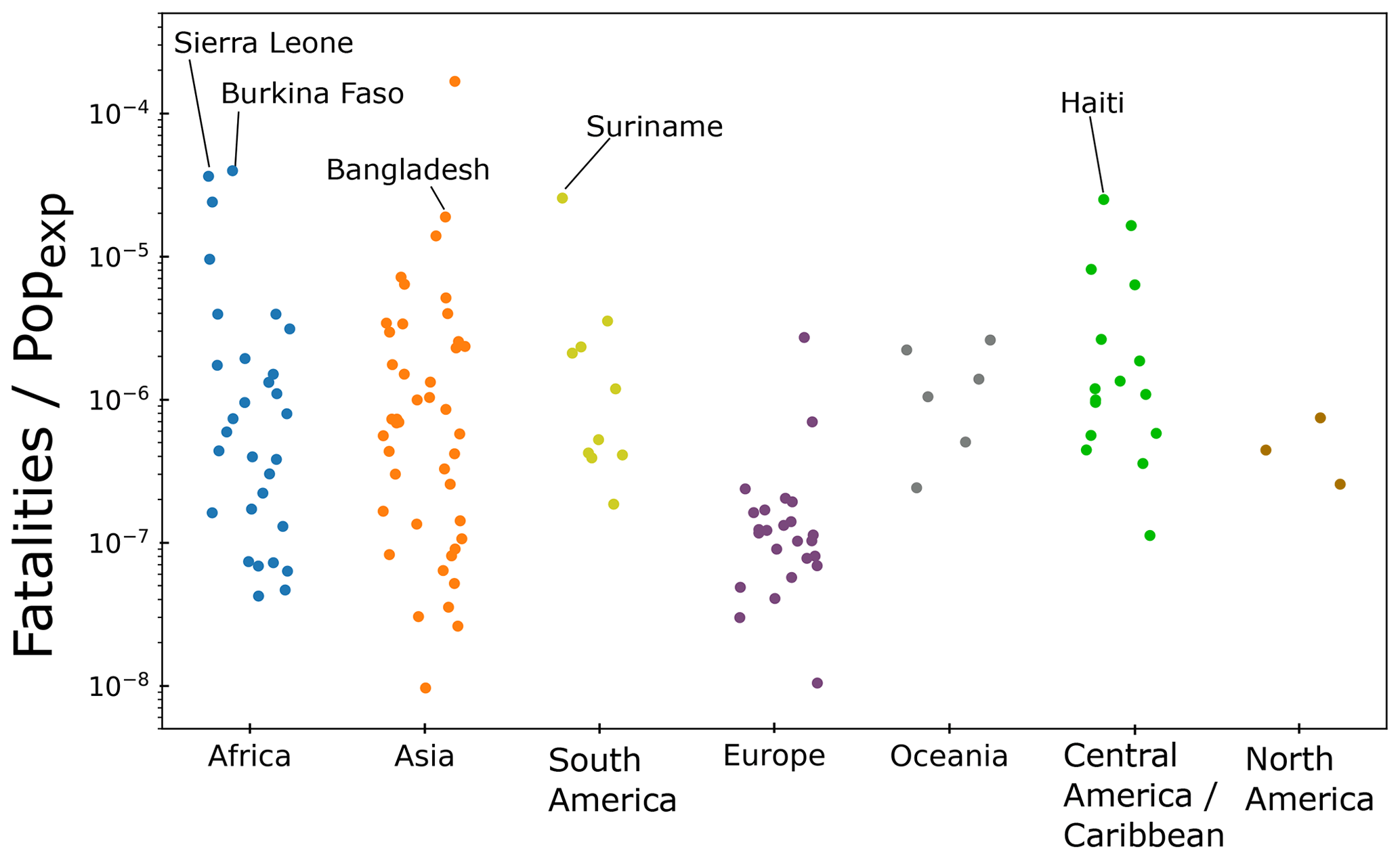
Figure 7Number of fatalities divided by Popexp, for each continent. The wide spread of values in Africa and Asia is likely a reflection of the diversity of nation-to-nation landslide vulnerability. Offsets on the x axis are for visual distinction between points to avoid overlap.
At the other end of the spectrum, some less developed countries exhibit higher fatalities for a given exposure; Sierra Leone, Burkina Faso, Haiti, Suriname, Bangladesh, Dominica and the Philippines have a significantly higher level of fatalities per unit of exposure. Some key outliers (Qatar and Bahrain) have high fatalities per unit exposure, but these nations have very low overall exposure (see Table S1), meaning that even a small number of fatalities increases the y-axis value in Fig. 7 to a large degree. This analysis, while not at this stage comprehensive, potentially allows us to explore a proxy for national-level risk management associated with landslide hazard, or relative vulnerability to a given level of exposure
To explore whether the variability in fatalities divided by Popexp seen in Fig. 7 is related to the level of development in each country, we have compared fatalities divided by Popexp with 2018 GDP values for each country (World Bank, 2018b). A priori, we would expect countries with greater GDP to be capable of mitigating hazard more effectively and thus have fewer fatalities for a given level of exposure. However, while there is a small average decline in fatalities for a given exposure as GDP increases (Fig. 8), with some high-GDP countries showing the lowest fatality values (notably Germany and Hong Kong), there is a significant degree of variability in this relationship, suggesting there is a more complex relationship.

Figure 8Gross domestic product per capita (World Bank, 2018) compared with the number of landslide fatalities per unit exposure.
We note that comparing the model-based estimates of exposure with the fatality inventory of Froude and Petley (2018) in this manner may lead to erroneous conclusions if not considered carefully. While it is likely that many, if not all, of the fatal landslides in developed countries are accurately recorded, this may not be the case in states where disaster management is less advanced. As such the lack of a strong relationship between fatalities per unit exposure and GDP per capita observed in Fig. 8 may represent gaps in the data in countries with lower GDP per capita, and thus a systematic bias within this analysis. Phrased differently, there may still be a relationship between GDP and fatalities for a given exposure level, but this may be masked by a lower reporting capacity in less developed nations.
While these results provide an independent estimate of landslide hazard and exposure across the globe that does not rely on a specific inventory, there are still assumptions and limitations that should be considered to put these results in appropriate context.
The most important caveat associated with these data is that nowcasts do not represent a guarantee of a landslide. The LHASA model nowcasts (Kirschbaum and Stanley, 2018) are issued when there is an increased likelihood of a rainfall-triggered landslide, meaning the estimates of exposure represent the relative likelihood of exposure to landslides, rather than the reported impacts. As such, nowcast number is a proxy for landslide hazard, rather than a quantifiable landslide hazard. However, we suggest that this disadvantage is more than offset by the global homogeneity and comparability of the nowcast output. In addition, since the nowcast-based estimates of hazard are based on historical rainfall data, they do not provide effective prediction of future exposure to hazard. This is particularly important given the potential for climate change to affect rainfall-driven hazards (Kleinen and Petschel-Held, 2007). Our model estimates of exposure would also fail to capture rainfall-driven exposure to landslide hazards in periods outside of the IMERG v06B record (pre 2001), including major rainfall-driven landslide events resulting from the 1998 El Niño event (Coe et al., 2004; Ngecu and Mathu, 1999). We stress that the model outputs are representative of the historical period under analysis, rather than strictly speaking a long-term average.
Additionally, since we do not have global data to quantify the vulnerability of settlements and infrastructure to landslide hazard, we cannot quantify the risk and impacts associated with landslide hazard. For example, data on fatalities associated with landsliding (Froude and Petley, 2018; Petley, 2012) quantify the impacts, and, while we can express our outputs in terms of relative proportion of population exposed to hazard, the lack of vulnerability data in our study represents an unconstrained source of variability if we compare those two datasets. Moreover, since the nowcast output does not capture information about the size of a potential landslide in a given area, there may be differences in the severity of the landslide events that occur depending on local factors (e.g. topography).
We note that we do not identify specific hospitals or schools as exposed to landslides. The resolution of our analysis remains coarse for individual points, and identifying specific locations could lead to overconfidence in exposure estimates. We acknowledge the importance of downscaling exposure estimates to those points and suggest it is another important future direction for landslide exposure estimation.
The resolution of the nowcast data also presents challenges to the interpretation. While a nowcast estimate for a 30 arcsec×30 arcsec grid cell provides an estimate of the landslide hazard therein, it does not provide information about where exactly a landslide may occur. Since infrastructure and population are unlikely to be evenly distributed within a grid cell (and are likely to be located further from areas of highest landslide susceptibility if risk mitigation measures have been adopted), elements that we describe as “exposed to landslide hazard” may never actually be so. Given the resolution of our input hazard data, we suggest that it is challenging to provide a more finely resolved estimate. This does highlight the need for effective downscaling methods that can be applied to coarse-resolution rainfall data to assess local landslide hazard. We hope to address this in future work. In addition, the LHASA model only models rapid landslide failures in natural settings. This means it does not capture landslides resulting from anthropogenic influence or slow-moving landslide events, which lead to a significant number of fatalities every year (Petley, 2012). Constraining exposure to this kind of failure is another important subject for future studies.
The value of a homogenous global dataset is highlighted when comparing the relative exposure of population to landslide hazard based on our estimates with the GDP cost associated with landslides derived from Dilley et al. (2005). The prior study is based upon the EM-DAT inventory of damaging landslides, but the complete absence of data for countries in sub-Saharan Africa (see Table S1) contrasts strongly with our results, which suggest that there is a significant proportion of the population in many sub-Saharan African countries exposed to landslide hazard.
Through combining rainfall, topography and other satellite-derived data, we have developed a long-term estimate of landslide hazard across the globe, which we have utilised to estimate the exposure of population and infrastructure to rainfall-induced landslides. These estimates are globally consistent and compare favourably with existing global datasets. When using them in conjunction with datasets of landslide fatalities, we can provide a nuanced picture of where and when landslides are most impactful. Our data highlight the importance of landslides in small mountainous nations and islands; while the absolute numbers of fatalities may be smaller, these represent locations with extremely high hazard and exposure. Further work is necessary to both test these results in a range of settings and to explore how global estimates can be downscaled and compared to more local estimates.
All material necessary to replicate these results can be found in the Supplement.
The supplement related to this article is available online at: https://doi.org/10.5194/nhess-20-3413-2020-supplement.
All authors were involved in study conceptualisation and writing of the manuscript. RE and TS carried out modelling and analysis.
The authors declare that they have no conflict of interest.
This article is part of the special issue “Global- and continental-scale risk assessment for natural hazards: methods and practice”. It is a result of the European Geosciences Union General Assembly 2018, Vienna, Austria, 8–13 April 2018.
Dalia Kirschbaum and Thomas Stanley are supported by the NASA Disasters Program. Robert Emberson is supported by a NASA Postdoctoral Fellowship administered by the Goddard Space Flight Center.
This research has been supported by the NASA Disasters Program (grant no. 18-DISASTER18-0022).
This paper was edited by Philip Ward and reviewed by Kate Allstadt and one anonymous referee.
Barrington-Leigh, C. and Millard-Ball, A.: The world' s user-generated road map is more than 80 % complete, PLoS One, 12, e0180698, https://doi.org/10.1371/journal.pone.0180698, 2017.
Carrao, H., Naumann, G., and Barbosa, P.: Mapping global patterns of drought risk: An empirical framework based on sub-national estimates of hazard, exposure and vulnerability, Global Environ. Chang., 39, 108–124, https://doi.org/10.1016/j.gloenvcha.2016.04.012, 2016.
Coe, B. J. A., Godt, J. W., and Tachker, P.: Map showing recent (1997–98 El Niño) and historical landslides, Crow Creek and vicinity, Alameda and Contra Costa Counties, California, US Department of the Interior, US Geological Survey, Denver, CO, https://doi.org/10.3133/sim2859, 2004.
De Bono, A. and Chatenoux, B.: A Global Exposure Model for GAR 2015, Background Paper prepared for the 2015 Global Assessment Report on Disaster Risk Reduction, UNEP/Grid, Geneva, 1–20, 2014.
Dilley, M., Chen, R. S., Deichmann, U., Lerner-Lam, A. L., Arnold, M., Agwe, J., Buys, P., Kjekstad, O., Lyon, B., and Gregory, Y.: Natural Disaster Hotspots A Global Risk Analysis, Disaster Risk Management Series, https://doi.org/10.1596/0-8213-5930-4, 2005.
Doxsey-Whitfield, E., MacManus, K., Adamo, S. B., Pistolesi, L., Squires, J., Borkovska, O., and Baptista, S. R.: Taking Advantage of the Improved Availability of Census Data: A First Look at the Gridded Population of the World, Version 4, Papers in Applied Geography, 1, 226–234, https://doi.org/10.1080/23754931.2015.1014272, 2015.
Froude, M. J. and Petley, D. N.: Global fatal landslide occurrence from 2004 to 2016, Nat. Hazards Earth Syst. Sci., 18, 2161–2181, https://doi.org/10.5194/nhess-18-2161-2018, 2018.
Guha-Sapir, D. and CRED (Centre for Research on the Epidemiology of Disasters): EM-DAT: The Emergency Events Database, Brussels, Belgium, available at: https://www.emdat.be/ (last access: 10 August 2018), 2019.
Haklay, M.: How good is volunteered geographical information? A comparative study of OpenStreetMap and Ordnance Survey datasets, Environ. Plann. B, 37, 682–703, https://doi.org/10.1068/b35097, 2010.
Kirschbaum, D. and Stanley, T.: Satellite-Based Assessment of Rainfall-Triggered Landslide Hazard for Situational Awareness, Earth's Future, 6, 505–523, https://doi.org/10.1002/2017EF000715, 2018.
Kirschbaum, D. B., Adler, R., Hong, Y., Hill, S., and Lerner-Lam, A.: A global landslide catalog for hazard applications: method, results, and limitations, Nat. Hazards, 52, 561–575, https://doi.org/10.1007/s11069-009-9401-4, 2010.
Kleinen, T. and Petschel-Held, G.: Integrated assessment of changes in flooding probabilities due to climate change, Climatic Change, 81, 283–312, https://doi.org/10.1007/s10584-006-9159-6, 2007.
Meijer, J. R., Huijbregts, M. A. J., Schotten, K. C. G. J., and Schipper, A. M.: Global patterns of current and future road infrastructure, Environ. Res. Lett., 13, 064006, https://doi.org/10.1088/1748-9326/aabd42, 2018.
Monsieurs, E., Jacobs, L., Michellier, C., Basimike Tchangaboba, J., Ganza, G. B., Kervyn, F., Mateso, J.-C. M., Bibentyo, T. M., Buzera, C. K., Nahimana, L., Ndayisenga, A., Nkurunziz, P., Thiery, W., Demoulin, A., Kervyn, M., and Dewitte, O.: Landslide inventory for hazard assessment in a data-poor context: a regional-scale approach in a tropical African environment, Landslides, 15, 2195–2209, https://doi.org/10.1007/s10346-018-1008-y, 2018.
Mooney, P., Corcoran, P., and Winstanley, A. C.: Towards Quality Metrics for OpenStreetMap, in: GIS '10: 18th SIGSPATIAL International Conference on Advances in Geographic Information Systems, San Jose, California, Association for Computing Machinery, New York, NY, USA, 514–517, November 2010.
Ngecu, W. M. and Mathu, E. M.: The El-Nino-triggered landslides and their socioeconomic impact on Kenya, Environ. Geol., 38, 277–284, https://doi.org/10.1007/s002540050425, 1999.
OpenStreetMap contributors: Planet dump, data file, available at: https://planet.openstreetmap.org (last access: 24 June 2019), 2015.
Petley, D: Global patterns of loss of life from landslides, Geology, 40, 927–930, https://doi.org/10.1130/G33217.1, 2012.
Petley, D. N., Hearn, G. J., Hart, A., Rosser, N. J., Dunning, S. A., Oven, K., and Mitchell, W. A.: Trends in landslide occurrence in Nepal, Nat. Hazards, 43, 23–44, https://doi.org/10.1007/s11069-006-9100-3, 2007.
Stanley, T. A. and Kirschbaum, D. B.: A heuristic approach to global landslide susceptibility mapping, Nat. Hazards, 87, 1–20, https://doi.org/10.1007/s11069-017-2757-y, 2017.
World Bank: “Population, total” World Development Indicators, The World Bank Group, available at: https://data.worldbank.org/indicator/SP.POP.TOTL (last access: 27 August, 2019), 2018a.
World Bank: “GDP (current US$)” World Development Indicators, The World Bank Group, available at: https://data.worldbank.org/indicator/NY.GDP.MKTP.CD (last access: 27 August, 2019), 2018b.