Modeling dependence and coincidence of storm surges and high tide: methodology, discussion and recommendations based on a simplified case study in Le Havre (France)

Coastal facilities such as nuclear power plants (NPPs) have to be designed to withstand extreme weather conditions and must, in particular, be protected against coastal floods because it is the most important source of coastal lowland inundations. Indeed, considering the combination of tide and extreme storm surges (SSs) is a key issue in the evaluation of the risk associated with coastal flooding hazard. Most existing studies are generally based on the assumption that high tides and extreme SSs are independent. While there are several approaches to analyze and characterize coastal flooding hazard with either extreme SSs or sea levels, only few studies propose and compare several approaches combining the tide density with the SS variable. Thus this study aims to develop a method for modeling dependence and coincidence of SSs and high tide. In this work, we have used existing methods for tide and SS combination and tried to improve the results by proposing a new alternative approach while showing the limitations and advantages of each method. Indeed, in order to estimate extreme sea levels, the classic joint probability method (JPM) is used by making use of a convolution between tide and the skew storm surge (SSS). Another statistical indirect analysis using the maximum instantaneous storm surge (MSS) is proposed in this paper as an alternative to the first method with the SSS variable. A direct frequency analysis using the extreme total sea level is also used as a reference method. The question we are trying to answer in this paper is then the coincidence and dependency essential for a combined tide and SS hazard analysis. The results brought to light a bias in the MSS-based procedure compared to the direct statistics on sea levels, and this bias is more important for high return periods. It was also concluded that an appropriate coincidence probability concept, considering the dependence structure between SSs, is needed for a better assessment of the risk using the MSS. The city of Le Havre in France was used as a case study. Overall, the example has shown that the return level (RL) estimates using the MSS variable are quite different from those obtained with the method using the SSSs, with acceptable uncertainty. Furthermore, the shape parameter is negative from all the methods with a much heavier tail when the SSS and the extreme sea levels (ESLs) are used as variables of interest.

1 Introduction

Like any other urban facilities, nuclear power plants (NPPs) can be subject to external influences and aggressions such as extreme environmental events (e.g., river and/or marine flooding, heat spells). Both nuclear and urban facilities have to be designed to withstand extreme weather conditions. During the last few decades, France has experienced several violent storms (e.g., the Great Storm of 1987, Lothar and Martin cyclones in 1999, Klaus in 2009, and Xynthia in 2010) that gave rise to exceptional storm surges (SSs). Many coastal facilities were partially or completely flooded when Storm Martin struck the French coast in 1999. A combination of an exceptional SS, of a high tide and high waves induced by strong winds led to the overflow of many dikes which were not designed for such a concomitance of events (Mattéi et al., 2001). In the nuclear safety field for instance, a guide to protection, including some fundamental changes in the assessment of flood risks, has therefore been produced by the Nuclear Safety Authority (ASN, 2013). However, to be conservative, approaches used in the guide are deterministic, which do not take into account all the local specificities of each site. The safety demonstration and protections are periodically reviewed to ensure compliance with the increased safety requirements. The present work could be used to enrich safety verification approaches, by proposing other approaches and confronting them to the reference method currently used in the guide. To supplement knowledge which can be acquired from the deterministic method, the probabilistic approach has been identified as an effective tool for assessing risk associated with hazards as well as for estimating uncertainties.

The first probabilistic study in the nuclear safety field was conducted in the United States in 1975 (US-NRC, 1975). This report focused on estimating the probability of occurrence of meltdown accidents with associated radiological consequences. Currently, probabilistic approaches are applied in several fields such as medicine, chemical industry, insurance and aeronautics. Many studies have already been conducted for the seismic hazard (IAEA, 1993; Beauval, 2003; Gupta, 2007), the tsunami hazard (IRSN, 2015) and other climatic hazards such as tornadoes (US-NRC, 2007). There are not many probabilistic studies yet in the fields of climate and hydrometeorology, as it is an approach barely used. In fact, very few studies and developments are explicitly referred to by their authors as conclusive and operational. Probabilistic flood hazard assessment (PFHA) is identified by Bensi and Kanney (2015) as a first step in a probabilistic risk assessment (PRA). According to the authors, it is an evaluation of the probabilities that one or more parameters representing the severity of the external flood (water level, duration and associated effects) are exceeded at a site of interest. Also, the authors discuss the joint probability method (JPM) as an alternative to existing deterministic and statistical methods such as the empirical simulation technique (EST). Klügel (2013) proposed a methodology for characterizing the external flood hazard for nuclear sites located alongside rivers and the articulation of this hazard study with a flooding probabilistic safety assessment (PSA).

It is a common belief today that the probability of failure, over an infrastructure lifetime, is one of the most important pieces of information an engineer can communicate. The estimation of the probability of exceeding an extreme event should be based on the combination of all flood sources (e.g., pluvial, fluvial and coastal floods) which are most often dependent because they are induced by the same storm. Mostly, a flood phenomenon can be characterized by several explanatory variables, some of which are correlated. The problem of the surge–tide interactions has been addressed in the literature for many regions and with different approaches (Coles and Tawn, 2005; Gouldby et al., 2014; Pirazzoli and Tomasin, 2007; Idier et al., 2012; Idier et al., 2019). It was shown that tide–surge interactions can be relevant in several regions. The tide–surge interactions at the Bay of Bengal (corresponding to the effect of the tide on atmospheric surge and vice versa) were analyzed by Johns et al. (1985) and Krien et al. (2017). They showed that tide–surge interactions in shallow areas of this large deltaic zone in the range ± 0.6 m occurred at a maximum of 1 to 2 h after low tide. Similar results were obtained by Johns et al. (1985), Antony and Unnikrishnan (2013), and more recently Hussain and Tajima (2017). Focusing on the English Channel, Idier et al. (2012) used a shallow-water model to make surge computations with and without tide for two selected events (November 2007 North Sea and March 2008 Atlantic storms). The authors concluded that the instantaneous tide–surge interactions are significant in the eastern half of the English Channel, reaching values of 74 cm in the Dover Strait, which is about half of maximal storm surges induced by the same events. They also concluded that skew surges are tide-dependent, with negligible values (less than 5 cm) over a large portion of the English Channel but reaching several tens of centimeters in some locations such as the Isle of Wight and Dover Strait. More recently, Idier et al. (2019) have investigated the interactions between the sea level components (sea level rise, tides, storm surges, etc.), and the tide effect on atmospheric storm surges is among the main interactions investigated in their review. The authors stated that the studies, and other ones, converge to highlight that tide–surge interactions can produce tens of centimeters of water level at the coast.

On the other hand, there are some phenomena which are described by other explanatory phenomena. The the case of multi-component phenomena, which will receive our attention in the present paper, is coastal flooding, which is a combination of tides with SSs. Indeed, SS is one of the main drivers of coastal floods. It is an abnormal rise of water generated by a storm (low atmospheric pressure and strong winds), over and above the predicted tide. It should be noted that the effect of waves (runup and setup) on total water level is not discussed in the present paper. Extreme storms can produce high sea levels, especially when they coincide with high tide. The skew storm surge (SSS) is a sea level component which is often considered the fundamental input or the quantity of interest for statistical investigations of coastal hazards. It is the difference between the highest observed level and the highest predicted one, for a same high tide. These maximum levels can occur at slightly different times.

As more than one explanatory variable are often used in a PFHA and in the case these variables are dependent, the dependency structure must be modeled and a consistent theoretical framework must be introduced for the calculation of the return periods and design quantiles with multivariate analysis based on copulas (e.g., Salvadori et al., 2011). Indeed, numerous studies have shown that, in the case of multivariate hazards, a univariate frequency analysis does not allow the estimation in a complete way of the probability of occurrence of an extreme event (Chebana and Ouarda, 2011; Hamdi et al., 2016). According to Salvadori and De Michele (2004), modeling the dependency allows a better understanding of the hazard and avoids under-/overestimating the risk. Unsurprisingly, some ideas have been proposed in the literature for combining tides and SSs and to help address such an important issue. JPM is an indirect method that made an improvement in addressing the main limitations of the direct methods (e.g., the annual maxima method (AMM) and the r-largest method (RLM)) (Haigh et al., 2010). Several studies refer to the JPM for the probabilistic characterization of storms (Batstone et al., 2013; Haigh et al., 2010; Pugh and Vassie, 1978; USACE, 2015). Tawn and Vassie (1989) proposed a revised JPM (RJPM) in which the distribution of surges is composed of a left tail defined by an empirical method and a right tail defined by frequency analysis. Dixon and Tawn (1994) made some modifications on the RJPM and proposed a new model to take into account the interaction between instantaneous SS and tide. Recently, Haigh et al. (2010) showed the advantages of indirect methods (i.e., JPM, RJPM) compared to direct ones (i.e., AMM and RLM). More recently, Kergadallan et al. (2014) proposed an extension of the model proposed by Dixon and Tawn (1994) using skew storm surges (SSSs) at 19 French harbors along the Atlantic and English Channel coasts of France. The authors have used two different approaches (the seasonal dependence and the interaction between SSs and tides) to study the dependence of the SSs on the tides with three methods (the seasonal approach, Dixon and Tawn, 1994 model and the revisited Dixon and Tawn model). It was concluded that the interaction between SSSs and high tides affect more significantly the results than the seasonal dependence for more than one-half of the harbors.

Some other studies have been proposed in the literature to tackle the PFHA. The most important contribution proposes two methods. The first estimates extreme sea levels (ESLs) with the JPM (Pugh and Vassie, 1980). Indeed, this approach combines separated frequency distributions for the tide (usually deterministic and exact) and the SS (frequency analysis based on the extreme value theory). It is a calculation of the convolution based on the tidal level density function and of a distribution function of SSs. Duluc et al. (2012) have shown that the quality of the results from this convolution approach for small return periods is questionable. The second procedure uses the data of observed maximum water levels (Chen et al., 2014; Haigh et al., 2014; Huang et al., 2008). This approach was recommended by FEMA's guideline (FEMA, 2004) for coastal flood mapping, in which the generalize extreme value model is recommended to conduct the frequency analysis of extreme water levels, if long-term datasets are available. Based on the regional observations, the process of estimation of extreme water levels uses an adequate frequency analysis model to estimate the distribution parameters, the desired return levels (RLs) and associated confidence intervals.

Overall, our goal is to build on the approaches and developments proposed in the literature and revive the debate as to how researchers and engineers can combine tide with SS to estimate extreme sea levels. This goal is in line with the recent literature (e.g., Idier et al., 2012; Kergadallan et al., 2014) challenging the use of the SSS and clearly demonstrates the importance of using the maximum instantaneous surge (MSS) instead. In order to achieve this goal, a third fitting procedure to estimate extreme sea levels using the MSS between two consecutive high tides is introduced with an application so that it can be compared with the two first procedures. Mazas et al. (2014) proposed a review of tide–surge interaction methods and applied a POT frequency model (with the generalized Pareto distribution (GPD) and Poisson distribution functions) to the family of JPM-type approaches for determining extreme sea level values in a single case study (Brest). The authors focused on the use of a mixture model for the surge component, which allows probabilities to be quantified for the entire range of sea level values, not just for the extreme ones, which is not the case here in the present paper.

The paper is organized as follows. Section 2 takes up the two fitting procedures proposed in the literature (the JPM with a convolution between tides and SSSs and the frequency analysis directly on sea levels) and proposes a new one based on the convolution between tides and MSSs. In Sect. 3, the fitting procedures are applied on the observed and predicted sea levels at the Le Havre tide gauge in France used as a case study. One of the most important features of this case study is the fact that the lower parts of Le Havre are likely to be flooded by coastal floods and that the region has experienced important storms during the last few decades.

2 Methods

Tide and SSs are usually the subject of a statistical study to determine the probability of exceeding the water level cumulating the two phenomena. Indeed, the SS is the main driver of coastal flood events. It is an abnormal rise of water generated by a storm, over and above the predicted tide. As it will be analyzed later in the discussion section, the dependency, in an extreme value context, is analyzed but not considered to combine the phenomena in the present work. Indeed, as mentioned in the introductory section and as it will be discussed later in this paper, extreme levels such as MSSs and high tides may be only very weakly dependent.

On the other hand, it is commonly known that the tidal signals can be predicted and are not aleatory like the SSs. What is somewhat odd in the present work is that one thus seeks to combine a distribution function of random variable with a density of tide which is deterministic. In order to estimate extreme sea levels, a JPM is used by making use of a convolution between tide and SSs. So the question that arises here is which variable of interest can be used to better characterize coastal flooding. Three variables are then proposed: (i) the SSS, (ii) the MSS and (iii) the extreme sea level. The theoretical basis for the fitting procedures using these variables is addressed in the following subsections.

Relative to some chosen datum, each hourly observed sea level Z(t) may be considered the sum of its tide X(t) and storm surge component Y(t), i.e.,

$$\begin{array}{}\text{(1)}& Z\left(t\right)=X\left(t\right)+Y\left(t\right).\end{array}$$

Thus if the probability density functions of the tidal and surge components are f_X(X) and f_Y(y) respectively. Then the probability density function f(z) of z, under the assumption that the tide and surge components are independent, is

$$\begin{array}{}\text{(2)}& f_Z\left(z\right)=\underset{-\mathrm{\infty }}{\overset{+\mathrm{\infty }}{\int }}{f}_X\left(X\right)\times f_Y\left(z-x\right)\mathrm{d}x.\end{array}$$

As can be seen in Eq. (2), the dependence on time, t, is omitted when replacing X(t) by X, Y(t) by Y, and Z(t) by Z. This implies a stationarity assumption for the involved time series. The hourly SS is often considered a stationary stochastic process, since meteorological and seasonal effects give rise to series of SSs randomly distributed in time, but this is not the case for the hourly theoretical tide signals. It should also be noted that, for the case of Le Havre, the residual part of the surges is not the only one. Despite the fact that it is the dominant component, the stochastic signal also contains the fluvial effects.

2.1 Joint SSS–tide probabilistic method

This method is based on the decomposition of the sea level into a sum of two contributions: the tide which is evaluated theoretically and the aleatory component SS obtained by subtracting the predicted tide from the observed sea level. Extreme storms can produce high sea levels, especially when it occurs simultaneously with high tide. The SSS is a sea level component which is often considered the fundamental input for statistical investigations of coastal hazards. It is defined as the difference between two observed and predicted maximums and is not impacted by the shift of the two signals which may be biased (see Fig. 1). As shown in the left panel of Fig. 2, the SSS is defined herein as the difference between the highest observed level and the highest predicted one, for the same high tide (see Eqs. 1 and 2). Further noteworthy features of SSSs are its occurrence with a high tide. Indeed, a SSS occurring with a high tide is likely to induce a high sea level. Thus, for safety requirements, SSS is the most often used in the literature (Kergadallan et al., 2014).

Figure 1 Definition and schematic representation of a skew storm surge.

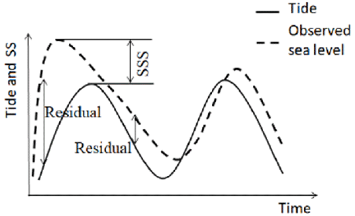
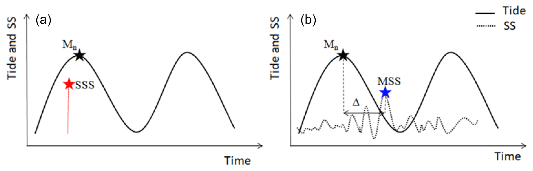
Figure 2 Illustration of tide and storm surge signals for the of joint surge–tide probability procedures: (a) skew surge–tide combination; (b) maximum surge–tide combination.

Still, even if this procedure uses the suitable variable of interest, it has its limitations. Indeed, it is not uncommon that the MSS, which can occur randomly somewhere between two consecutive tides, is greater than the SSS. Widening the window around the high tide, in which extreme SSs are extracted, could improve frequency estimation of extreme sea levels. When this window is maximum (12 h, for instance), the variable of interest naturally becomes the MSS. Moreover, it was demonstrated in the literature that the tide and SSS interaction at high tide cannot be neglected (Kergadallan et al., 2014).

2.2 Joint MSS–tide probabilistic method

Figure 2a illustrates the case of an instantaneous SS signal; the variables would be the MSS and the high tide M_n. As mentioned in the previous section, the MSS can occur randomly somewhere in a tide cycle. One of the most important features of MSS is that it is more informative than the SSS. Indeed, the MSS covers the whole instantaneous SS signal. This feature makes the MSS a variable particularly useful for carrying out a PFHA exploring the entire tidal signal, not only the high tide.

2.3 Inference with the ESL: the reference method

For comparison purposes, we also analyzed sea levels signals for which we focused our attention on the frequency analysis on extreme sea levels without decomposing them into tides and surges. This yields to direct statistics and estimates of the RLs without combining tides and surges. The intent of this analysis is only to illustrate and obtain results that can serve as a reference for the comparison of the joint probability procedures. The maximum sea level between two high-tide values is the variable of interest used for this reference procedure.

2.4 The sampling method

The peaks-over-threshold (POT) sampling method is used to conduct the frequency analyses in the present work. Commonly considered an alternative to the annual maxima method, the POT method models the peaks exceeding a relatively high threshold. The distribution of these peaks converges to the GPD theoretical distribution. In addition, the threshold leads to a sample more representative of extreme events (Coles, 2001). However, the threshold selection is subjective, and an optimal threshold is difficult to obtain. Indeed, a threshold that is too low can introduce a bias in the estimation because some observations may not be extreme data, and this violates the principle of the extreme value theory. On the one hand, the use of a threshold that is too high reduces the sample size (Hamdi et al., 2014).

On the other hand, all the simulations were carried out within the R environment (open-source software for statistical computing: http://www.r-project.org/, last access: 15 Novemeber 2020). The SeaLev library, developed by the French Institute for Radiological Protection and Nuclear Safety (IRSN), was used for the standard approach involving the convolution of the probability density functions of the tidal and surge heights to obtain the distribution of total sea levels. The frequency analyses were performed with the Renext library also developed by IRSN (IRSN and Alpstat, 2013). The Renext package was specifically developed for flood frequency analyses using the POT method.

3 Case study and data

The city of Le Havre is an urban city in the Seine-Maritime department, on the English Channel coast in Normandy (France). It is a major French city located in northwestern France. A map showing the location of the city of Le Havre in France can be found in Fig. 3. The name Le Havre means “the harbor” or “the port”. The port of Le Havre is, moreover, among the largest in France. For these reasons, the city of Le Havre remains deeply influenced by its maritime traditions.

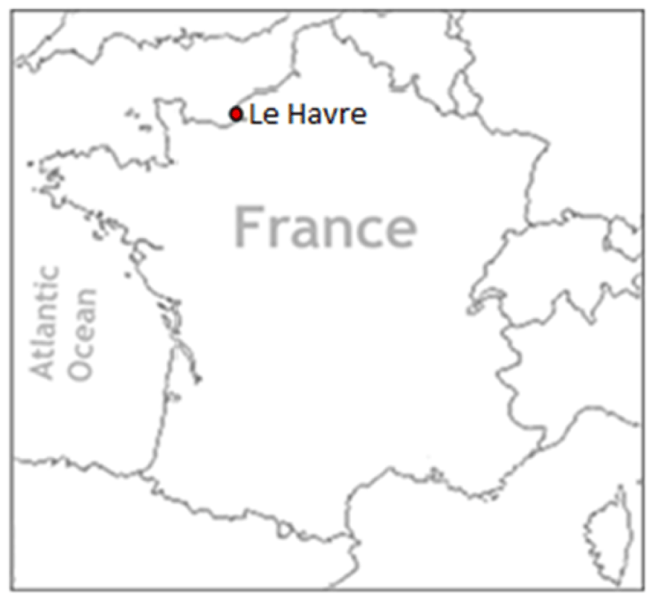
Figure 3 Case study (Le Havre): location map.

Due to its location on the coast of the English Channel, the climate of Le Havre is temperate oceanic. Days without wind are rare. There are maritime influences throughout the year. According to the meteorological records, precipitation is distributed throughout the year, with a maximum in autumn and winter. The months of June and July are marked by some relatively extreme storms on average 2 d per month. One of the characteristics of the region is the high variability of the temperature, even during the day. The prevailing winds are from north-northeast for breezes and from the southwest sector for strong winds.

The joint tide–surge probability and the frequency analysis of extreme sea levels are performed on the city of Le Havre. The 1971–2015 observed and predicted hourly sea levels recorded at the port of Le Havre were provided by the French Oceanographic Service (SHOM – Service Hydrographique et Océanographique de la Marine). Figure 4 shows the sea level time series of Le Havre, as well as the studied extreme SSs (SSSs and MSSs). One of the most important features of Le Havre is the fact that it is subject to marine submersions and instabilities of coastal cliffs (Elineau et al., 2010, 2013; Maspataud et al., 2016). In particular, the lower part of the city (Saint-François district, for instance) is likely to be flooded by marine and pluvial floods. Data characteristics are shown in the Table 1. These data were first processed to keep only common periods containing a minimum of gaps. The choice of the variables to be probabilized is done at this stage.

Table 1 Sea level and rainfall datasets.

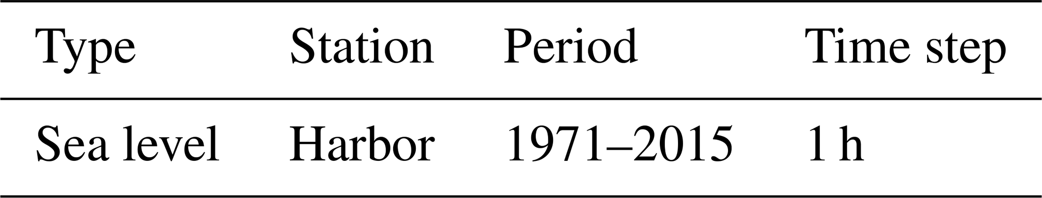
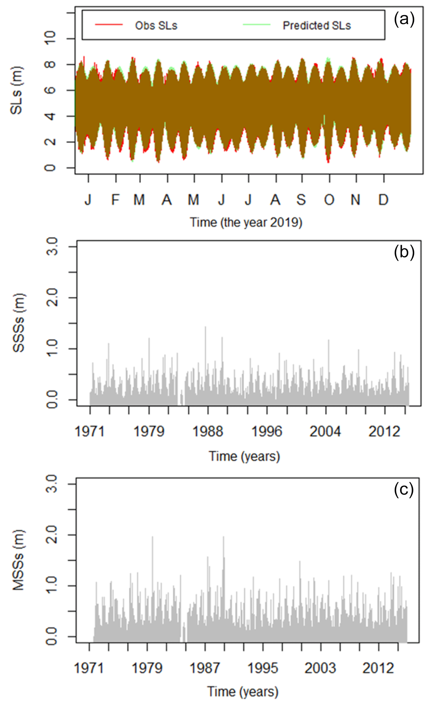
Figure 4 Studied time series of Le Havre: (a) predicted and observed sea levels; (b) SSS data and (c) the MSSs.

4 Results

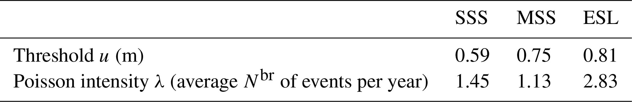
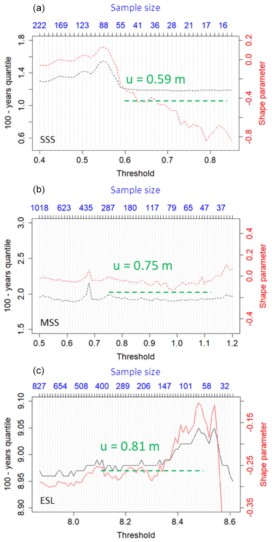
Since we need to get comparable annual rates of extreme sea level events, the POT threshold selection process has been adapted to meet this criterion. The thresholds are, however, checked regarding the stability graphs of the GPD parameters estimated with the maximum likelihood method. The POT model characteristics (threshold and associated average number of events per year) are presented in Table 2. The stability graphs for threshold selection are presented in Fig. 5.

Table 2 POT thresholds for SSS, MSS and ESL variables.

Figure 5 Stability plots for threshold selection: (a) SSSs, (b) MSSs and (c) ESL.

The main results of the joint surge–tide probability method, with the SSS- and MSS-based fitting procedures, and the results of the direct frequency analysis of the extreme sea levels as well, with all the diagnostics, are presented in terms of RL plots, estimates of the quantiles of interest and associated 95 % confidence intervals. In these results, the main focus was set to the 10-, 50-, 100- and 1000-year sea level RLs. Prior to the application of the JPM, the SSSs and MSSs are calculated first from observed and predicted sea levels. The results of the application on the Le Havre are summarized in Table 3 and presented in Fig. 6.

Table 3 Sea RLs and 95 % confidence intervals for the three fitting procedures (in meters).

Figure 6 Sea level quantiles and confidence intervals.

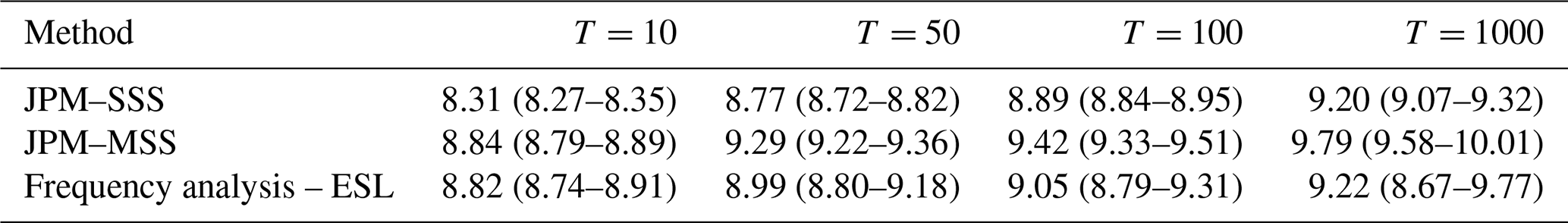
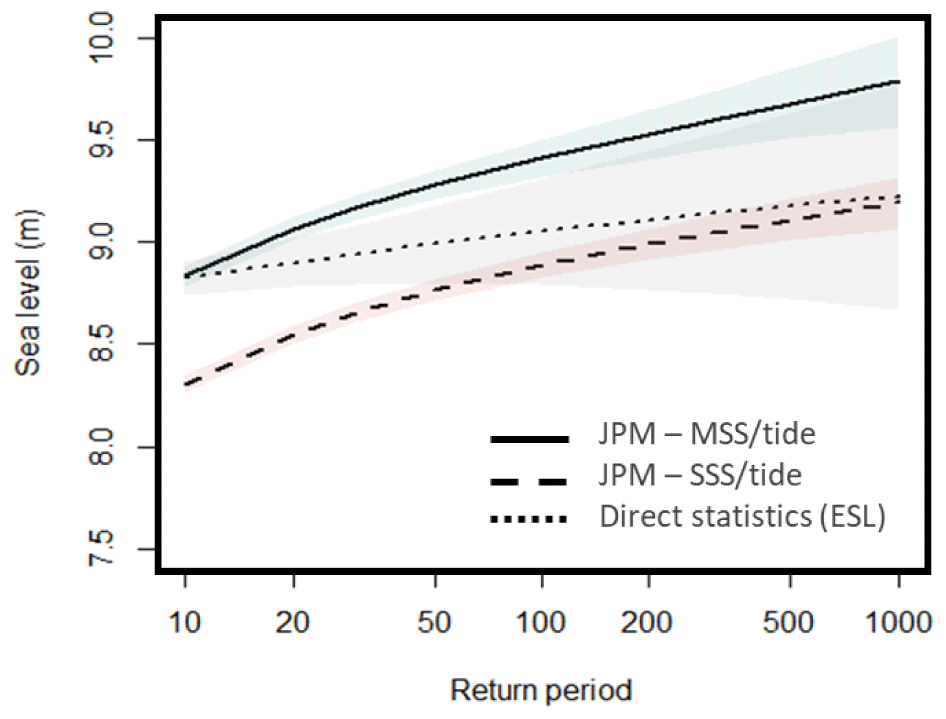
The RL estimates obtained with the MSS-based convolution are quite different from those of the one based on SSSs. The results of the calculation of confidence intervals (with the delta method) are presented with transparent polygons in Fig. 6 and in Table 3 as well. As it can be noticed, the confidence intervals are relatively narrow. Indeed, the relative width of the intervals around the 1000-year RL obtained with reference method did not exceed 12 %. Better yet, the confidence intervals are narrower when using the joint probability procedures. It is interesting to note that the delta method (Ver Hoef, 2012) is a classic technique in statistics for computing confidence intervals for functions of maximum-likelihood estimates. The variance of RL estimates is calculated using an asymptotic approximation to the normal distribution. Furthermore, it can be seen in Fig. 6 that for a given RL, the return period given by the MSS-based procedure is much lower than that given by the one based on the SSSs. The RLs are thus more frequently (i.e., on average 10 times more frequently) exceeded randomly in a tidal cycle (i.e., as the MSS can occur randomly somewhere inside a tidal cycle) than at the high-tide moment (i.e., if we suppose that SSS often occurs at the high-tide moment).

It is noteworthy that the shape parameter ξ of the GPD is negative for all the cases (i.e., $\mathit{\xi }=-\mathrm{0.2}$; $\mathit{\xi }=-\mathrm{0.07}$ and $\mathit{\xi }=-\mathrm{0.12}$ for the SSS-, MSS- and ESL-based fitting procedures, respectively). This parameter governs the tail behavior of the GPD. The right tail of the distribution is much heavier for the procedures using SSSs and the ESLs than for the one using MSSs.

5 Discussion

To objectively evaluate the merits and shortcomings of each of the methods described in Sect. 2, the associated assumptions must be analyzed first. The JPM is developed under the assumption of independence between the tidal signal and SSs. Tawn and Vassie (1989) found that this assumption was false. Consider that this assumption may be true under certain circumstances as proven by Williams et al. (2016) for the largest midlatitude storm surges and the corresponding tide. A tendency to overestimate sea levels, due to the fact that the correlation between tide SSs has been ignored, was recognized in the literature (Pugh and Vassie, 1978, 1980; Walden et al., 1982). However, it should be noticed that extreme levels such as the MSSs may be only very weakly dependent with high tides. This constitutes a distinctive feature and advantage of the MSS-based fitting procedure introduced in the present paper. It is a major point of differentiation between the joint surge–tide probability procedures described in Sect. 2. Furthermore, the hourly theoretical tides are in utmost cases considered a realization of the stationary process. This assumption is the most critical one since sea levels are highly non-stationary due to storm surge. As previously argued to overcome this limitation, the variability arises from the SSs, which can be considered stationary over the storm season for instance. For this argument to be less subjective, most high tides are similar in terms of their value and must be lower than the SS variation in extreme events.

The question one can ask is how to improve the modeling in such a way that the bias between the procedures using SSSs and MSSs and the reference one is reduced as much as possible. Indeed, as depicted in Fig. 6, the second procedure overestimates extreme sea levels for all the return periods (a maximizing envelope). The RL estimates for MSS-based procedure are about 50 to 60 cm higher than those obtained when the SSS are used. The difference between the upper and middle curves increases as the return period goes up. The difference is high for high return periods. Inversely, the difference between the lower and middle curves increases as the return period goes down. The difference is significant for lower return periods. It is noteworthy that the middle curve is supposed to represent the RLs of reference. An objective answer to our question cannot in any case suggest a modification in the reference method. Two methodological issues could provide us with solutions and answers to the question. First, the dependence structure that exists between the high tide and the extreme SSs around the high tide could be modeled. Extreme SSs 1 h before the high tide, at the time of the high tide and 1 h after can be used. A larger window can likewise be used to consider the SSs around the high tide in a multivariate context.

A visual inspection with the scatter graphs and Spearman's ρ numerical criteria have been used to measure the statistical dependence between storm surges and tide at the moment of the high tide and around it (± 1 h). This is useful when modeling the coincidence of the high tide with extreme storm surges, for instance. The multivariate frequency analysis consists in studying the dependence structure of two or more variables through a function that depends on their marginal distribution functions. The multivariate theory is based on the mathematical concept of copula (Sklar, 1959), which allows linking the distributions of the variables according to their degree of dependence. More details can be found in Salvadori and De Michele (2004) and Nelsen (2006). A copula-based approach may be used to consider this dependence. In the case of a copula of sea levels, no convolution is needed. The convolution of SS distribution with a density of tide permits obtaining a distribution of sea levels. This latter solution is proposed herein as an alternative to the multivariate analysis using a copula.

The Fig. 7 shows the scatter graphs that provide a visual information about the dependence between the high tide and the other variables (SSS, MSS and ESL). It can be concluded that the dependence with the two storm surge variables SSS and MSS is weak and sufficiently low to consider the variables statistically independent. This finding is supported by Spearman's ρ coefficients, and associated p values are presented in Table 4. Indeed, to determine whether a correlation between the variables is significant or not, we need to conduct a Pearson correlation test and compare the p value to a significance level. In general, a significance level of 0.05 gives good results. This value of α indicates the risk of concluding that there is a correlation when in reality there is none is 5 %. As a matter of fact, the p value is nothing other than the probability that the correlation coefficient is significantly different from 0. However, the Pearson coefficients are very close to zero for the SSS and MSS variables, and a zero coefficient indicates that there is no linear dependence, whatever the p value. A p value is presented for each variable in Table 4. As Spearman's coefficients only correspond to one facet of dependence and to better analyze the association between the SSs and high tide, Kendall's correlation coefficient is used as well. It is often of interest in data analysis and methodological research and similar to Spearman's correlation coefficient; it is designed to capture the association between two variables. Results of Kendall's τ test, also presented in Table 4, also support the statistical significance of non-dependence between SSs and tide. The two sea level components (high tide and extreme SSs) are then considered independent random variables, and the distribution of the total sea level can be determined by convolution. Otherwise, a multivariate analysis based on the use of the copulas theory can be used.

Table 4 Spearman's ρ coefficients (and associated p values) as a measure of dependence between the tide and the other variables.

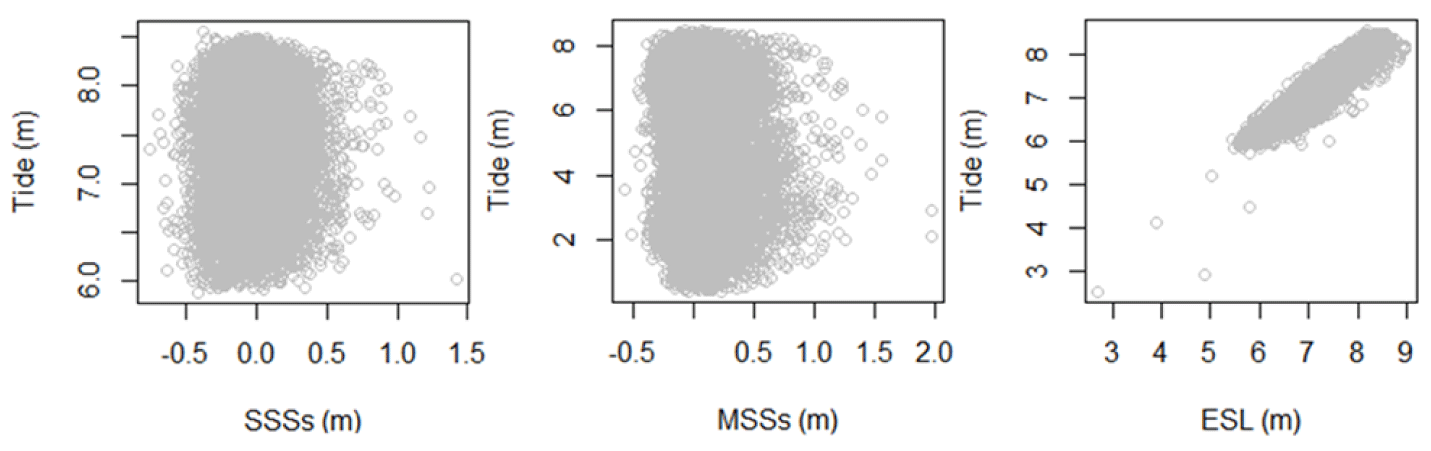
Figure 7 Analysis of the dependence between the tide and the SSSs, the MSSs and the ESL events.

6 Further discussion

As shown in Fig. 6, RLs obtained with the joint MSS–tide method are always higher than those using SSS. This is consistent with the fact that the convolution process based on MSS uses only high water values for the tide density (as it selects the maximum value of instantaneous SSs every 12 h) and since MSS is always greater than or equal to SSS. It is then logical to consider that the joint MSS–tide method is more conservative than the SSS-based one. As expected, Fig. 4 shows that ESL events at the right tail of the distribution, represented by the middle curve, tend to be close to high SSS RLs which are dominated by the high tide. The results of this procedure confirm the general finding highlighted in the literature (Fortunato et al., 2016; Haigh et al., 2016) that the return level estimations obtained with the convolution tide–SSS are not adapted up to a certain return period (100 years in the case of Le Havre). To overcome this problem, one can use the joint tide–MSS convolution method. Another solution is to use an empirical method to define the left tail of the distribution and an extreme value analysis for the right tail as stated by Tawn and Vassie (1989).

On the other hand, the current practices and statistical approaches to characterize the coastal flooding hazard by estimating extreme storm surges and sea levels still have some weaknesses. Indeed, the combination of the tide and the storm surge does not take into account several scenarios, in particular those with a time lag where the tide and the storm surge could likewise give extreme sea levels. The choice of variables (high tide, SSS, MSS, etc.) would be a decisive step and an integral part of the logic behind the idea of combining the two phenomena. Interestingly, these variables could also include other explanatory variables such as the time lag between the two phenomena (tide and SS). This time lag would be an additional variable, and it is defined as the difference of time of occurrence of the second variable with respect to the first (e.g., time between a maximum storm surge and a high tide).

6.1 Coincidence probability concept

Our interest to the probability of coincidence comes from our belief that a bias is introduced with the joint-MSS convolution because it does not take into account the time difference between the maximum instantaneous SS and the high tide. A probability of coincidence (i.e., the chance that a MSS occurs at the same time with high tide) can be used to better characterize the extreme sea levels using the MSS. In the present paper, we are only interested in the concept of the coincidence probability and the statistical dependence between MSS and tide at the moment of the high tide and around it (± 6 h). An appropriate coincidence probability concept would then allow a better estimation of the probabilities and thus would reduce the bias and bring the RLs closer to those obtained by the reference method.

Let Δ be the time lag between the high tide and the MSSs in each tide cycle. When considering coincidence, an additional hazard curve associated with the variable Δ can be built. The time lag variable Δ, which would allow us to compute a probability of coincidence, could be involved in a multivariate frequency analysis to consider the dependence structure between the variables. It is also interesting to note that the probability of coincidence would make it possible to conclude whether the MSSs occur randomly in a tide cycle or not. The work must be performed for many coastal systems with different physical properties to conclude whether or not there is a systematic temporal dependence and whether or not the extreme sea levels are overestimated if this is indeed the case.

As illustrated in Fig. 2b the MSS can occur randomly somewhere around the high tide M_n. The time difference between the MSS and the high tide is random as well. It is therefore quite legitimate to study it with a frequency analysis method. Then a coincidence probability concept can be drawn as follows:

•  

  Extract an independent sample of Δ.

•  

  Fit this sample with the appropriate distribution function. Indeed, Δ is expressed in hours, and it is not an extreme variable; it is bounded between −6 h and 6 h and can take any value with in this interval. There is then no tail of the distribution, and the extreme value theory is not the appropriate framework to model this random variable. Thus, a uniform distribution would be a good fit for Δ.

•  

  Use the desired probability to weight the probabilities of the MSSs, assuming that MSSs and Δ are independent. Many scenarios using many of these probabilities can be used in a probabilistic approach.

On the other hand and focusing on the statistical dependence, extreme SS samples around the high tide (at the time Δ of the high tide) was extracted. The largest window (± 6 h) centered on the time of the high tide was used, and the statistical dependence was then studied. Table 5 shows Spearman's ρ measuring the statistical dependence between storm surges and tide at the moment of the high tide and around it (± 3 h). It can be easily concluded that the dependence between SSs and tides is very high around the time of high tide, and it becomes weaker as Δ increases. As mentioned in the previous section, the dependence structure that exists between the MSSs around the high tide could be modeled with copulas.

Table 5 Spearman's ρ calculated between high tide and all the instantaneous surges in the tidal cycle.

6.2 The non-stationary context

It is noteworthy that the climate change in the past and working in a non-stationary context can greatly affect and invalidate the fit of the storm surge and sea level probability density functions. Indeed, the following questions are fair and justified: what is the effect of potential trends and jumps in the sea water level time series and should this affect the results and its confidence? The non-stationary context is not covered by this paper because it moves us further away from the main objective, which is the use and the confrontation of different methods for quantifying the exceedance probability of extreme sea levels. It could however be the subject of another paper.

7 Conclusions

In the present paper, we provided a reasoning for the need, in a PFHA framework, to combine flood phenomena to better characterize coastal flooding hazard. Few ideas have been proposed in the literature to tackle the combination of tidal signals with extreme SSSs to estimate extreme sea levels. The present work supports these ideas, takes up the tidal signals and SSSs convolution procedure, and proposes a new procedure based on the MSSs useful to exploit likewise the extreme SS events that occurred during medium- and low-tide hours. Three fitting procedures have been investigated. The first one employs the SSS as an explanatory variable with the tidal signals which are combined with a JPM using a convolution of the tide density and the SSS distribution function. The second procedure uses the same technique except that the MSSs are used instead of the SSSs. In the third approach, a frequency analysis is performed using ESLs.

Another consideration in this paper was applying and illustrating these approaches on the example of the sea levels in Le Havre, northwestern France, over the period 1971–2015. It may be noted that the methodology is not exemplary developed for this case study; it applies to any site likely to experience marine flooding. Fitting results in terms of probability plots and extrapolated RLs using the three approaches are examined. Overall, the application has shown that the RL estimates for MSS-based convolution are quite different from those corresponding to the SSS-based one. Indeed, since MSS is always greater than or equal to SSS and since the convolution process using MSS selects the maximum value of instantaneous SSs every tidal cycle, the RLs are systematically higher when the joint MSS–tide method is used. But without properly tackling the probability of coincidence concept (i.e., the chance that a maximum SS occurs at the same time with high tide) and the issue of temporal lag between tidal peaks and surge peaks, the results will be probably always overestimated, which may not be useful for PFHA. the results of the MSS-based procedure are likely to contain a bias compared to the direct statistics on ESLs, which becomes more and more important as return periods increase. In order to reduce this bias, the coincidence probability concept could be helpful in making a more appropriate assessment of the risk using the MSS. On the other hand and if the MSS-based convolution is to be used, the application has shown the utility of modeling the dependence structure that exists between the hourly SS values around the high tide (high tide ± 6 h). Figure 6 shows that ESL events at the upper tail of the distribution (the middle curve) tend to occur at the time of the high tide, as expected. The results of this procedure confirm the general finding highlighted in the literature is that the RL estimations obtained with the convolution tide–SSS are not conclusive up to a certain return period (100 years in the case of Le Havre).

An in-depth study could help to thoroughly improve the proposed procedure based on the use of MSS by developing the concept of coincidence and applying the developed concept at other sites of interest. A concept of coincidence and methodology to be developed should find additional applications for the assessment of risk associated with other combining flooding phenomena (e.g., pluvial flooding and storm surges).