the Creative Commons Attribution 4.0 License.
the Creative Commons Attribution 4.0 License.
 | 03 Dec 2020
Laboratory study of non-linear wave–wave interactions of extreme focused waves in the nearshore zone
Iskander Abroug
Nizar Abcha
Armelle Jarno
François Marin
Extreme waves play a crucial role in marine inundation hazards and coastal erosion. Prediction of non-linear wave–wave interactions is crucial in assessing the propagation of shallow water extreme waves in coastal regions. In this article, we experimentally study non-linear wave–wave interactions of large-amplitude focused wave groups propagating in a two-dimensional wave flume over a mild slope (). The influence of the frequency spectrum and the steepness on the non-linear interactions of focused waves are examined. The generated wave trains correspond to Pierson–Moskowitz and JONSWAP (γ=3.3 or γ=7) spectra. Subsequently, we experimentally approach this problem by the use of a bispectral analysis applied on short time series, via the wavelet-based bicoherence parameter, which identifies and quantifies the phase coupling resulting from non-resonant or bound triad interactions with the peak frequency. The bispectral analysis shows that the phase coupling increases gradually and approaches 1 just prior to breaking, accordingly with the spectrum broadening and the energy increase in high-frequency components. Downstream breaking, the values of phase coupling between the peak frequency and its higher harmonics decrease drastically, and the bicoherence spectrum becomes less structured.
- Article
(7277 KB) - Full-text XML
-
Supplement
(3459 KB) - BibTeX
- EndNote


Extreme wave propagation is a highly non-linear process observed in both open seas and coastal regions. The main physical mechanisms which may lead to an extreme wave event are illustrated in Kharif and Pelinovsky (2003), Kharif et al. (2009), Didenkulova and Anderson (2010) and Onorato et al. (2013). Extreme waves may occur in deep or shallow water, in energetic storm sea state, or in a previously calm sea state. In our opinion, spatio-temporal wave focusing is one of the most important mechanisms in the extreme wave formation for shallow and deep water (Kharif and Pelinovsky, 2003). The spatio-temporal wave focusing is a classical mechanism giving rise to an important wave energy concentration in a small region. If the wave height of the focusing group exceeds 2.2 times its significant wave height, it can be defined as a rogue or freak wave (Dysthe et al., 2008). For this reason, spatio-temporal wave focusing is often employed in laboratory wave flumes with a wide variation of water depth (Merkoune et al., 2013), spectrum type (Tian et al., 2011; Xu et al., 2019; Abroug et al., 2019, 2020) and wavelength-to-depth ratio, in order to better understand the generation process, the dynamic behaviour and the hydrodynamic loads on ocean structures in extreme sea conditions.
Over the past years, several studies have attempted to quantify the spatial evolution of spectral energy of unidirectional wave groups in experimental wave flumes using a classic Fourier analysis (Tian et al., 2011; Liang et al., 2017; Abroug et al., 2020). The frequency spectrum only gives the distribution of energy in the frequency domain; however, information about the phase coupling between different wave components is unknown. Consequently, higher-order spectrum techniques should be adopted. A powerful tool to investigate the highly non-linear process is the wavelet-based bispectral technique, which has been used in several works to study the non-linear interactions and quadratic phase coupling between wave components (Dong et al., 2008; Ma et al., 2010). The need to detect and quantify second-order non-linear interactions can be found in many disciplines, such as geophysics (Grinsted et al., 2004), plasma physics (Milligen et al., 1995), fault diagnosis (Li et al., 2014), health-related areas, neuroscience (Bai et al., 2017) and wave analysis (Eldeberky, 1996; Eldeberky and Madsen, 1999; Young et al., 1996; Young and Eldeberky, 1998; Becq-Girard et al., 1999; Huseni and Balaji, 2017; Zhang et al., 2019). In wave analysis, the propagation of wave trains in the nearshore zone has an exceptionally high spectral and temporal resolution.
The majority of previous works regarding the evolution of unidirectional wave trains in numerical and experimental wave flumes have shown that spatio-temporal focusing leads to a shape and elevation of a wave crest at focus that cannot be predicted by either linear or second-order wave theory. This is due to high-order non-linearities, called the bound (harmonics) and resonant non-linearities (Vyzikas et al., 2018). On the one hand, bound non-linearities are the result of non-linear harmonics that are phase locked to the wave train and contribute in the sharpening of free surface elevation. On the other hand, resonant interactions contribute in the redistribution of energy among different frequency components. It is important to mention here that in shallow water regions exact resonant interactions are hardly realised in unidirectional propagation because the resonant conditions cannot be satisfied in a small area. Therefore, we investigate specifically the role of bound waves generated by non-resonant three-wave coupling.
Over the past few decades, various experimental studies have investigated the spatial evolution of non-linear coupling between wave components. Dong et al. (2008) studied the spatial evolution of non-linear interactions between different wave components in the shoaling and de-shoaling region by carrying out two random wave experiments based on JONSWAP spectra with varying peak wave periods and root-mean-square wave heights. They showed that the degree of quadratic phase coupling increases in the shoaling region and achieves its highest level prior to wave breaking. Ma et al. (2010) studied experimentally JONSWAP wave trains propagating in intermediate water depth. Recently, non-linear transformation of unidirectional irregular waves propagating over a complex bathymetry (; where kp is the peak wavenumber and h denotes the water depth) was performed in Zhang et al. (2019), who studied the triad wave–wave non-linear interactions in the case of long records of JONSWAP irregular waves (1200 Tp, where Tp is the peak period) using a Fourier-based bispectral analysis. They found that the phase coupling is strong near the end of the slope, where second and third harmonics become more important. They also noticed the appearance of low-frequency waves generated by the difference interactions during wave propagation. We must note here that the main difference between Fourier-based bicoherence and wavelet-based bicoherence is the number of degrees of freedom (Dong et al., 2008). Wavelet-based bicoherence is a suitable tool to detect non-linear wave–wave interactions occurring in relatively short data sequences and can be used to analyse data collected in laboratory flumes (Elsayed, 2006).
Most of the aforementioned studies were conducted in random wave conditions based on JONSWAP spectra. To the authors' knowledge, few studies have attempted to quantify the degree of phase coupling resulting from the propagation of realistic spectrum wave trains in the nearshore zone using wavelet-based bicoherence. Experiments are performed on numerous Pierson–Moskowitz and JONSWAP wave trains propagating from a constant intermediate water depth to shoaling and breaking zones.
The paper is outlined as follows. The experimental set-up and test conditions are illustrated in Sect. 2. In Sect. 3, a short formal description of wavelet analysis and wavelet-based bicoherence is provided. The spatial evolution of wavelet-based bicoherence is discussed in Sect. 4. Section 5 is devoted to conclusions and perspectives.
The following is a brief consideration of present wave trains generation; more details of the experiments can be found in Abroug et al., 2020. The experiments were conducted in a two-dimensional wave flume of the M2C (Morphodynamique Continentale et Côtière) laboratory at Caen University, France. The flume is 22 m long, 0.8 wide and the water depth is h0=0.3 m (Fig. 1). In this study, the relative water depth kph0<1.363 is verified, which means that the modulation instability effect can be neglected (Janssen and Onorato, 2007; Fedele et al., 2019). An Edinburgh Designs Ltd piston type wave maker is located at one end of the flume to implement wave trains using linear wave generation signal. Wave trains are generated with almost no reflection at the end of the flume, since measurements are performed before reflected waves travel back to the measurement location. Thus, the occurrence of resonant interactions potentially driven by reflected waves is limited, and we only focus on bound waves.
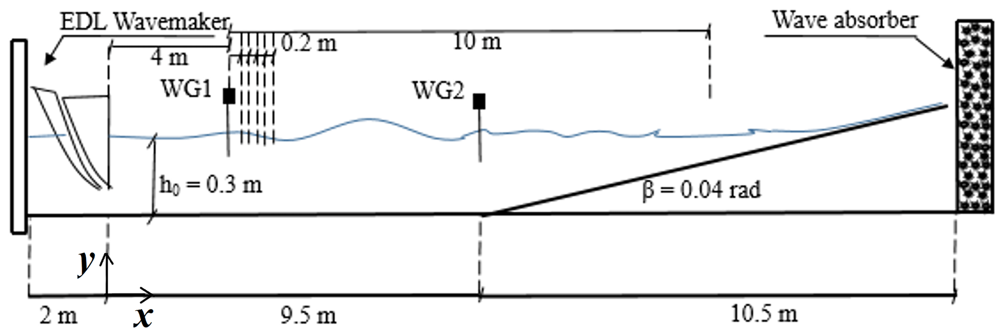
Figure 1Schematic experimental set-up: WG1 and WG2 denote wave gauge no. 1 and wave gauge no. 2 respectively.
The data used in this work are issued from Abroug et al. (2020). The present study relates to seven wave train simulations based on the averaged JONSWAP spectra (i.e. with peak factor γ=3.3 or 7) or Pierson–Moskowitz spectra with varied peak wave periods fp and wave steepnesses S0 (i.e. non-linearity). The linear NewWave theory (Tromans et al., 1991), which is able to generate targeted waves at a prescribed location and time by combining sinusoidal components of different frequencies, is used as input for the generated focused wave trains. This theory was validated at deep water locations, at intermediate water depth locations (Taylor and Williams, 2004) and at coastal regions (Whittaker et al., 2016); for kh<0.5). In NewWave theory, the expected shape of a wave train is the autocorrelation function (Fourier transform of the spectral density).
For each wave train, a large number of wave signals were recorded along the flume to accurately follow the wave evolution in space. The surface elevation is measured by two aligned wave gauges located from the longitudinal coordinate xmin=4 m to xmax=14 m, where x=0 is defined as the mean position of the wave maker. The positions of these wave gauges are clearly delineated in Fig. 1. The sampling rate is 50 Hz and each record duration is 35 s with a sample interval of 0.02 s. The fast Fourier transform (FFT) was applied to each signal, resulting in 1750 frequency components over the range [0, 3fp] and with a spectral resolution Δf=0.023 Hz. The distance from the wave maker for the focusing point was set to 12 m from the wave maker.
Using linear NewWave theory, the free surface elevation of a wave train at a distance x from the wave maker can be written as follows:
where ai (Eq. 2) is the amplitude of each component, i varies from 1 to N (number of waves), x0 and t0 denote respectively the predefined focal location and focal time, is the wavenumber, ωi=2πfi is the angular frequency, h is the water depth, A0 represents the theoretical linear crest amplitude of the wave train, S(fi) is the spectral density, and is the frequency step. JONSWAP and Pierson–Moskowitz are the two spectra used to represent the sea state. All generated waves are crested focused waves; i.e. the phase angle of the wave group within its envelope at the focus position is equal to zero.
Based on Eq. (1), the varied parameters during these experiments were the spectrum type (S(fi)) and the wave steepness S0. The peak frequency parameter was chosen in order to have a relative depth kph0 varying between 0.79 and 0.92 (deep side in Table 1). Deep and shallow sides in Table 1 represent respectively the flat bottom depth (4 m < x < 9.5 m) and the shallowest studied depth (x=14 m). Five of the studied wave trains have more than one breaking, and breaking locations xb are indicated as bracketed intervals in Table 1.

The free surface elevation of each wave train was studied through the bispectral analysis applied on short time series, via the wavelet-based bicoherence. The detailed characteristics of the wavelet-based bicoherence can be found in Milligen et al. (1995), and a brief introduction of this technique is given below. The continuous wavelet transform WT(a, τ) of a time series f(t) is calculated as
where the asterisk denotes the complex conjugate and ψa,τ (Eq. 4) represents the mother wavelet function dilated by a factor τ and scaled by a factor a, a>0. The latter parameter can be interpreted as the frequency inverse; i.e. . The wavelet transform can be interpreted as a series of bandpass filter of the time series with a mother wavelet function. We have chosen the Morlet wavelet as a mother wavelet function because it provides information about phase and amplitude, and it is adapted for capturing coherence between harmonic components. The Morlet wavelet can be considered as a modulated Gaussian waveform and is defined as
where ω0 denotes the dimensionless frequency and t is the dimensionless time. The Morlet wavelet with ω0=6 is a good choice, since it ensures a good balance between time and frequency localisation (Grinsted et al., 2004; Dong et al., 2008). For the Morlet wavelet the scale a is almost equal to the Fourier period T (T=1.03a). As mentioned in Dong et al. (2008), it is convenient to write the scales a as fractional powers of two (Torrence and Compo, 1998):
where a0 is the smallest resolvable scale, M represents the largest scale and δ denotes the scale factor. The a0 parameter should be chosen equal to 2×Δt (Torrence and Compo, 1998; Dong et al., 2008). N and Δt represent respectively the number of points in the times series and the time sampling. The scale factor δ should be sufficiently small to provide high resolution and adequate sampling in scale. Moreover, for the Morlet wavelet, a scale factor δ=0.5 is the largest value that gives adequate sampling (Dong et al., 2008). It is for that reason that we opted for a scale factor δ=0.02, giving a total of 395 scales ranging from 0.04 up to 11.83 for respectively high and low frequency. The wavelet-based bispectrum (Eq. 8) measures the phase coupling in the interval ΔT=35 s that occurs between f1, f2 and f3 where the latter parameters must satisfy the frequency sum rule (Eq. 9). Quadratic non-linear coupling occurs between f1 and f2, generating a third component at the sum frequency f3.
The bispectrum (Eq. 8), which is the double Fourier transform of the third-order moment, measures the extent of phase coherence due to the non-linear triad interaction between three waves that satisfy the frequency and phases matching criteria (Eqs. 9 and 10). The estimation of wavelet-based bispectrum in the whole bifrequency plan can be based on its values in the interval ψ: , Hz (Nyquist sampling frequency)}.
The wavelet-based bicoherence (Eq. 11), which can be defined as the normalised wavelet bispectrum, is used in practice to measure the degree of phase coupling (Larsen et al., 2001) and is bounded by 0 and 1 by the Schwarz inequality. A value close to unity reveals a maximum amount of coupling, and a value close to zero corresponds to a random phase relation.
Figure 2 exhibits a simple illustration of the wavelet-based bicoherence of a narrow-banded Gaussian wave train (Test 1) recorded at x=4 m from the wave maker. The shading indicates the strength of non-linear coupling, with dark red (b2(f1, f2)=1) being totally coupled and dark blue (b2(f1, f2)=0) completely uncoupled. The degree of phase coupling is represented by the colour bar indicating the sum interactions between two frequencies. In this manner, a visualisation of the non-linear activity across the wave train propagation is feasible, detecting the frequency sections of the signal that contribute the most to the non-linear activity. The two frequencies f1 and f2 are normalised by the peak frequency fp. Red (b2(fp, fp)) and yellow peaks represent the phase coupling of the primary frequency component with its harmonic. In general, a non-null bicoherence b2(f1, f2)>0 means that the component gains energy from the f1 and f2 components.
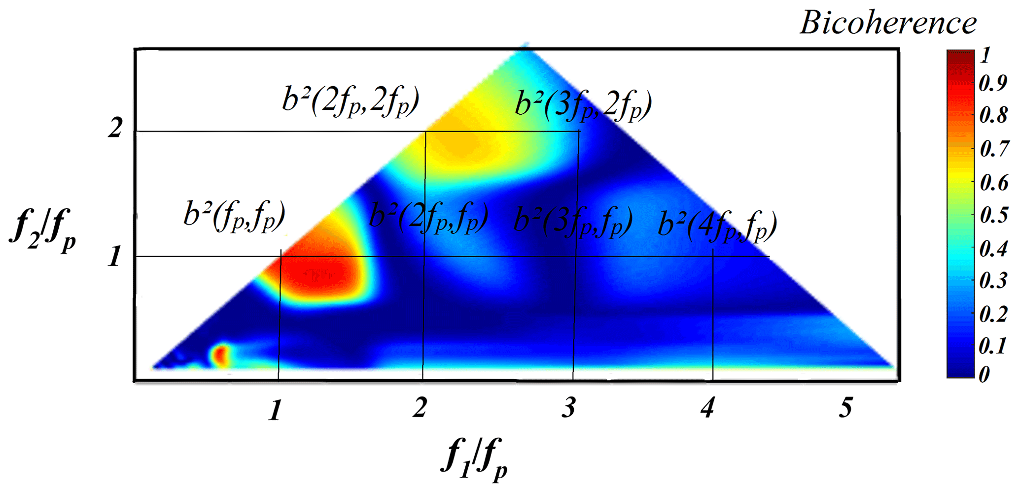
Figure 2The wavelet-based bicoherence of a narrow-banded Gaussian wave train (Test 1) at x=4 m.
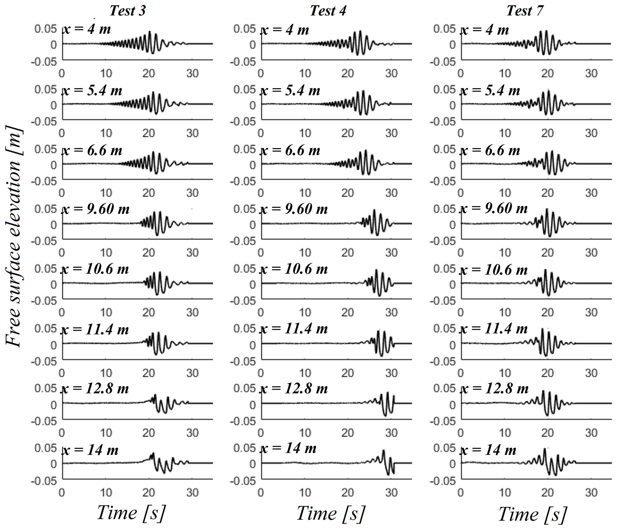
Figure 3Three sets of time series of Pierson–Moskowitz (Test 3), JONSWAP (γ=3.3) (Test 4) and JONSWAP (γ=7) (Test 7) wave trains.
Figure 3 shows three sets of time series of three wave trains with approximately the same steepness S0 and derived from Pierson–Moskowitz (Test 3; xb∈[11.09; 11.82]), JONSWAP (γ=3.3) (Test 4; xb∈[12.13; 12.81]) and JONSWAP (γ=7) (Test 7; xb∈[12.07; 12.69]) spectra at eight different locations along the flume. This preliminary figure shows surface elevation time histories including the first measurement (x=4 m), the propagation along the flat bottom, the shoaling and the breaking of the focused wave group. It should be noted here that the seven studied wave trains are crest-focused wave groups (Φ=0).
Figure 4 shows, in a log scale, the spatial evolution of the Fourier spectra of the same three wave trains (Test 3, 4 and 7). A spatial downshift of the spectral peak (Test 4 and 7), a steepening of the low-frequency side and a widening of the high-frequency side are illustrated. These spectral variations, identified and quantified in Abroug et al. (2020), concern high- and low-frequency components. The shift of energy is essentially due to non-linear wave–wave interactions among wave frequency components during the focalisation process. Nevertheless, we do not distinguish which wave components participate in the wave–wave interactions, nor do we distinguish the wave modes that undergo the strongest non-linear interactions. Consequently, the wavelet-based bicoherence is used herein to provide information about the non-linear triad wave interactions that cannot be easily obtained from the Fourier analysis which was used in Abroug et al. (2020).
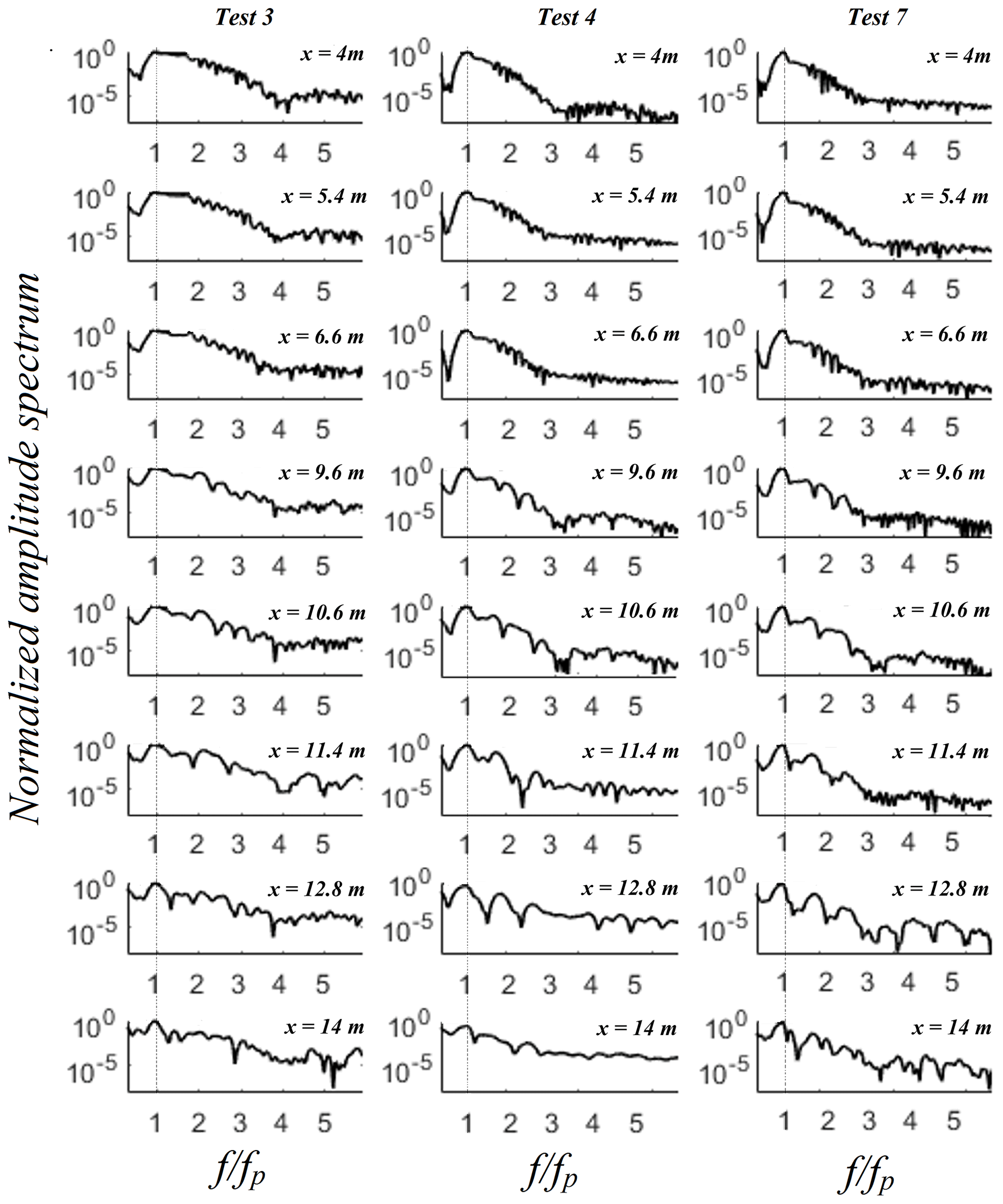
Figure 4Spatial evolution of normalised amplitude spectra in a log scale for Test 3, 4 and 7.
Figure 5 presents the spatial evolution of the wavelet-based bicoherence of a Pierson–Moskowitz wave train (Test 3; xb∈[11.09; 11.82]) along the flat bottom. This figure shows that wave–wave interactions between different modes are weak on flat bottom (4 m < x < 9.5 m; kph0=0.79), and few frequency components participate in the focusing process. In the intermediate water depth region (4 m < x < 9.5 m), the sea state is almost Gaussian, and for that reason non-linear wave–wave interactions are relatively moderate. For example, b2(fp, fp)=0.1 and b2(fp, 3fp)=0.065 at x=4 m indicate respectively a weak self–self wave interaction at the energy-frequency peak coupled with the energy at 2fp and a very weak wave interaction at the peak frequency coupled with the energy at 4fp (Fig. 5a). A significant bicoherence magnitude band ranging from 0.5fp to fp is observed, i.e. b2(0.5fp−fp, 0.5fp−fp), which indicates an energy transfer from low-frequency components to the spectral peak. This partially explains the spatial evolution of the spectrum, namely the increase in energy in the peak region, which is potentially a way of compensating for the energy dissipation in the transfer region, i.e. the region between the spectral peak and high-frequency regions (Abroug et al., 2020; Liang et al., 2017). Note that the magnitude of the bicoherence is consistent with the fact that spectrum shape does not vary substantially along the flat bottom (4 m < x < 9.5 m) (Fig. 4).
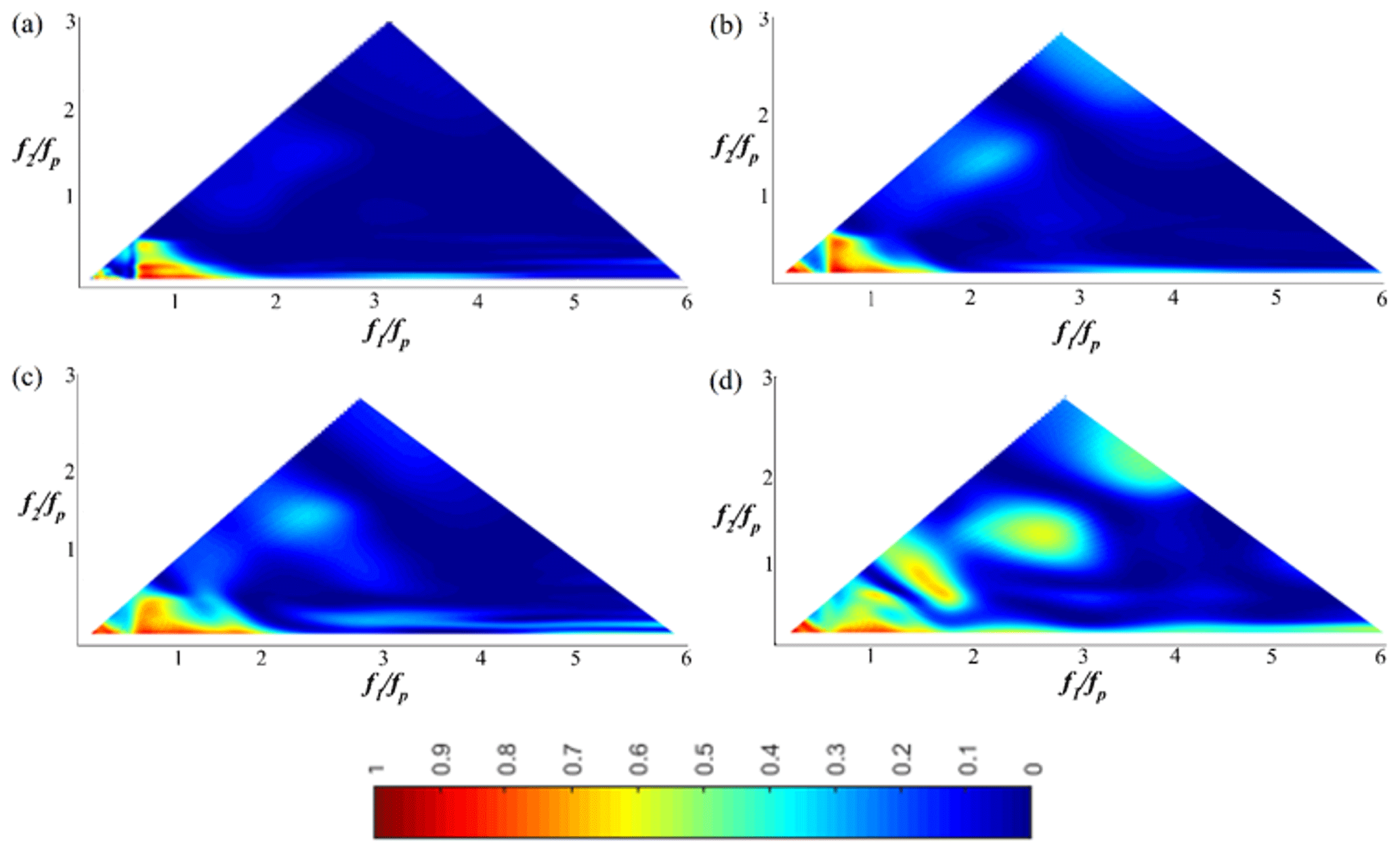
Figure 5The wavelet-based bicoherence spatial evolution on the flat bottom for a Pierson–Moskowitz wave train (Test 3). (a) x=4 m; (b) x=5 m; (c) x=8 m; (d) x=9.6 m.
As the wave train approaches the toe of the slope (x∼9.5 m), more and more wave components are involved in the non-linear phase coupling, and the bicoherence values increase progressively. For x=9.6 m, just a little over the toe of the slope, the bicoherence magnitude among primary components increases slightly, i.e. b2(fp, fp)=0.24 and b2(3fp, fp)=0.15, which is consistent with the small energy increase in the high-frequency region (Abroug et al., 2020).
As the wave train propagates in the shallower region (9.5 m < x < xb∈[11.09; 11.82]), the degree of phase coupling is seen to increase rapidly (Fig. 6a). The degree of phase coupling within the peak frequency increases considerably at shallower regions compared to deeper regions. Wave energy transfers increase in the high-frequency region, and as a result, the spectrum broadens. In the vicinity of the breaking location (xb∈[11.09; 11.82]), the non-linear coupling spreads over most of the wave components. The increase in the second and third harmonic is clearly noticeable in Fig. 6b. The values of bicoherence for approximately all frequency pairs are greater than 0.13, indicating that the non-linear coupling reaches its maximum level, which means that almost all of the higher harmonic waves are involved in the propagation process.
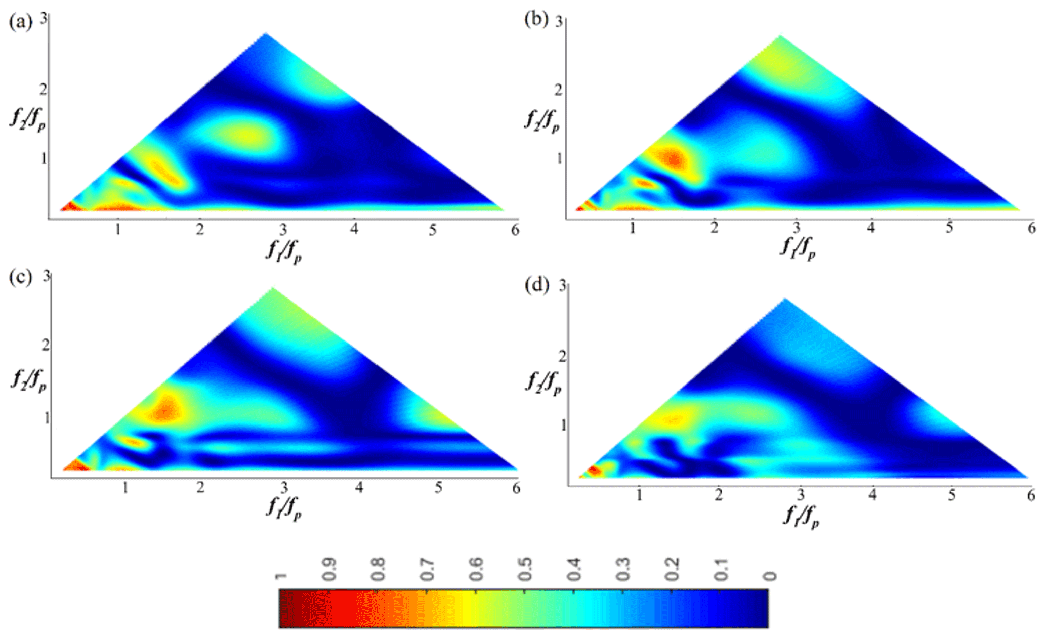
Figure 6The wavelet-based bicoherence spatial evolution on the sloping bottom for a Pierson–Moskowitz wave train (Test 3). (a) x=11 m; (b) x=12 m; (c) x=13 m; (d) x=13.8 m.
Downstream of the breaking location (11.09; 11.82]), the degree of phase coupling between frequency components decreases drastically, and the bicoherence becomes less structured (Fig. 6d). This result is consistent with the decreasing trend of energy in higher-frequency components downstream of the breaking location (Tian et al., 2011; Abroug et al., 2020).

Figure 7The wavelet-based bicoherence spatial evolution on the flat bottom for the JONSWAP (γ=3.3) wave train (Test 5). (a) x=4 m; (b) x=6 m; (c) x=8 m; (d) x=9.6.
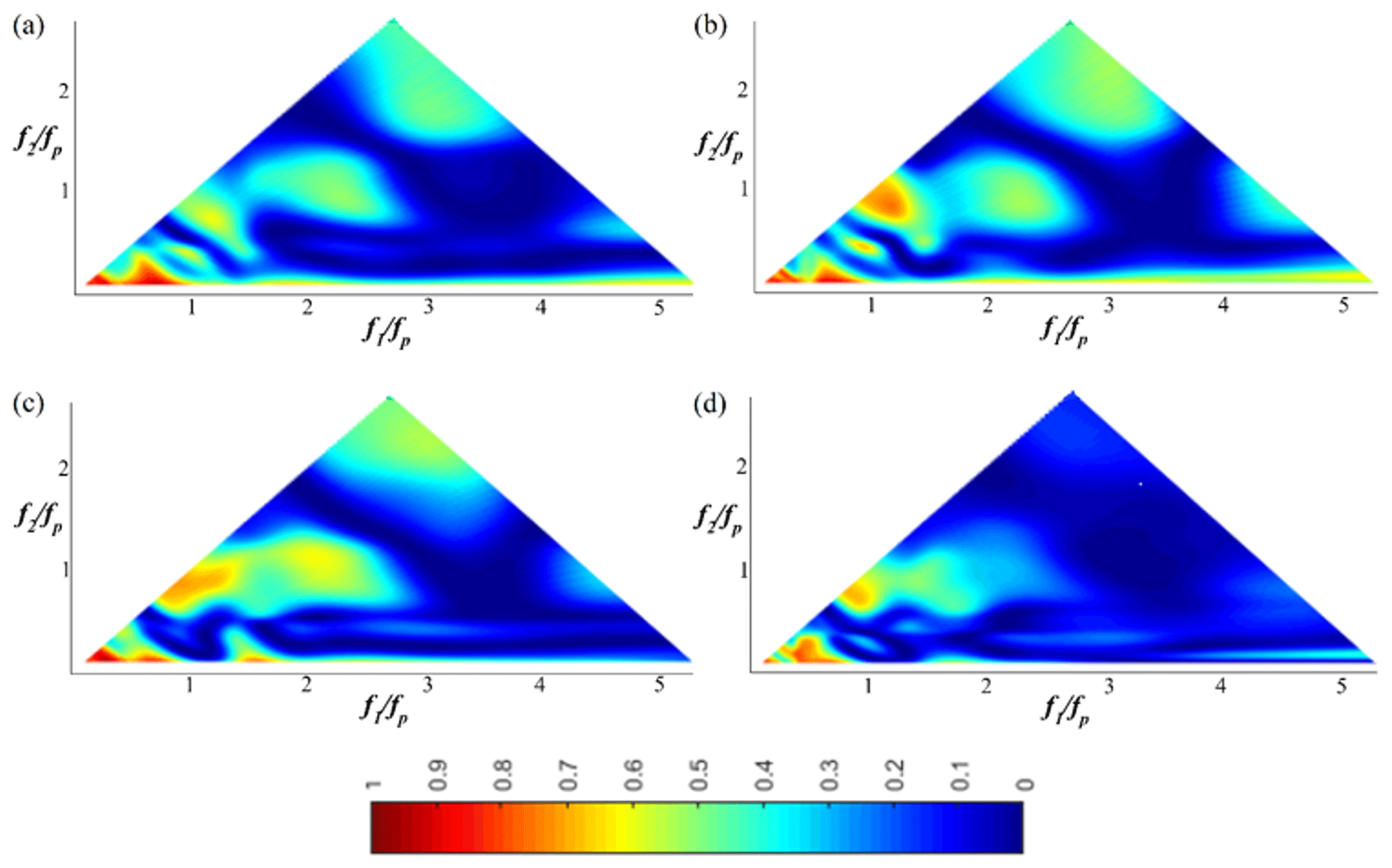
Figure 8The wavelet-based bicoherence spatial evolution on the sloping bottom for the JONSWAP (γ=3.3) wave train (Test 5). (a) x=10.20 m; (b) x=11.20 m; (c) x=12.40 m; (d) x=13.60 m.
In Figs. 7 and 8, a JONSWAP (γ=3.3) wave train (Test 5; xb∈[10.5; 11.61]) is chosen to illustrate the spatial evolution of the wavelet-based bicoherence of a narrower wave train propagating over the flat and the sloping bottom. Wave–wave interactions evolve qualitatively in the same way compared to the case of Pierson–Moskowitz. Figure 7a (x=4 m) shows that the two dominant phase coupling peaks appear at the bifrequencies (fp, fp) and (0.5fp, 0–0.5fp), which illustrates that the quadratic non-linear interactions only occur between the peak and low-frequency modes. Note that no other peak was found to be significant. As the wave train propagates over the shallower region (x>9.5 m), new phase couplings appear at the bifrequencies (2fp, fp), (3fp, fp) and (2fp, 3fp) (Fig. 8). This finding illustrates that quadratic non-linear interactions between the peak frequency, the first harmonic, and the second harmonic and third harmonic result from the gradual broadening of the spectrum. It is in accordance with previous studies demonstrating that energy is mainly transferred to high frequencies during the shoaling process (Tian et al., 2011; Liang et al., 2017; Abroug et al., 2020). For this wave train (Test 5), the wavelet-based bicoherence reaches its maximum shortly after the breaking (xb∈[10.5; 11.61]) at x=12 m. For example, b2(fp, fp)=0.7, b2(2fp, fp)=0.53 and b2(2fp, 2fp)=0.16. Triad interactions lead to skewed wave profiles and can characterise the near-breaking conditions (Fig. 3 for x>10.6 m).
Beyond the breaking location (; 11.61]), the bicoherence decreases sharply and becomes less structured. For example b2(fp, fp)=0.52, b2(2fp, fp)=0.31 and b2(2fp, 2fp)=0.004 at x=13.6 m; i.e. h=0.13 m. This pattern is qualitatively similar to that obtained in the case of a Pierson–Moskowitz wave train. This indicates that the increasing trend of the phase coupling is one of the more important reasons for the wave train breaking in shallow water.

Figure 9The wavelet-based bicoherence spatial evolution on the flat bottom for the JONSWAP (γ=7) wave train (Test 7). (a) x=4 m; (b) x=6.4 m; (c) x=8 m; (d) x=9.6 m.
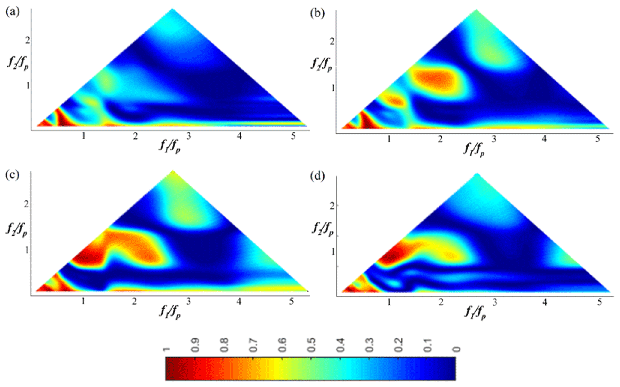
Figure 10The wavelet-based bicoherence spatial evolution on the sloping bottom for the JONSWAP (γ=7) wave train (Test 7). (a) x=10.2 m; (b) x=11 m; (c) x=12.4 m; (d) x=13.8 m.
Figures 9 and 10 depict the wavelet-based bicoherence spectra for the case of a JONSWAP (γ=7) wave train (Test 7; xb∈[12.07; 12.69]) at eight locations along the wave flume. No bispectral peak appears at b2(2fp, fp), and this is maybe not surprising as no clear third harmonic 3fp is present in the frequency spectrum (Fig. 4). Furthermore, wavelet-based bicoherence diagrams show that the phase coupling reaches its maximum level at frequencies slightly higher than the exact harmonics (2fp, 3fp …). This result is consistent with the results of Ma et al. (2010), who explained this process by the slight upshift of peak values in spectrum at higher harmonics, which is readily seen in Fig. 4. The fact that clear first, second and third harmonics are not present is possibly due to other mechanisms such as quadruplet interactions (, Elgar et al., 1995), which have a shape-stabilising impact on the spectrum and are confined to free waves. This result is consistent with the peak frequency downshift demonstrated experimentally in Stansberg (1994) and Abroug et al. (2020), where it was interpreted as a self-stabilising feature.
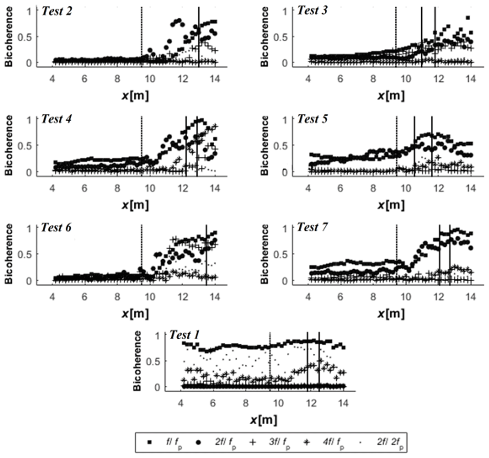
Figure 11Spatial variation of the wavelet-based bicoherence among harmonics. The two vertical solid lines and the dotted line respectively indicate the breaking region and the toe of the slope.
Figure 11 summarises the variability in the location and intensity of the wavelet-based bicoherence between the bifrequency pairs (fp, fp), (2fp, fp), (3fp, fp), (4fp, fp) and (2fp, 2fp) for several tests. The two vertical solid lines and the dotted line respectively indicate the breaking region and the toe of the slope. This figure indicates that the steepness has a strong influence on the non-linear phase coupling between harmonics in intermediate water depth (h0=0.3 m). Non-linear wave–wave interactions and their increasing trend is more important for wave trains having strong non-linearities. Beyond the wave breaking (x>xb), the decreasing trend of the phase coupling between harmonics is also more significant in the case of strong steepness S0. This result is in accordance with the dissipation related to breaking, which is particularly noticeable when the wave steepness is high (Abroug et al., 2020).
An important similarity between different spectra is that important wave–wave interactions are mostly limited to the first harmonics of primary waves (fp, fp) and (2fp, fp). This finding is consistent with the energetic behaviour of wave trains downstream of the wave breaking (Abroug et al., 2020). Moreover, in the case of small and moderate wave steepness (Test 2; xb=12.9 and Test 6; xb=13.5), the phase coupling varies slightly downstream of the wave breaking compared to that found prior to the breaking, suggesting that a small energy transfer happens downstream of the breaking location.
It can be concluded that bound or non-resonant interactions play an important role in the evolution and breaking of wave trains in shallow water depth. Although the bound waves are not supposed to contribute to the energy redistribution, our experimental observations raise the question of the impact of bound interactions on dissipation and energy transfers among different frequency components.
An experimental approach is proposed for determining the non-linear wave–wave interactions, which accompany the propagation of large amplitude wave trains, that might cause damage to coastal zones, marine structures and navigation vessels. We investigate seven focused wave trains derived from JONSWAP (γ=3.3 or 7) and Pierson–Moskowitz spectra propagating from intermediate water depth to the inner surf zone. The results presented in this study extend the parameter range of observations of triad interactions. The experimental conditions were selected based on two parameters: the wave steepness and the spectrum type. The present data were collected in intermediate water with a kph0 varying between 0.92 and 0.79. A typical wave train consists of a large number of waves interacting with one another. Wavelet-based bicoherence is used to investigate the phase coupling between frequency components of short time series. Some consequences of non-linear transfer are briefly discussed – in particular the role played by non-linear interactions in shaping the high-frequency part of the spectrum, the relative contribution of each harmonic and the downshifting of the peak spectrum demonstrated in previous studies. Note that our experimental study is different from previous experiments (Dong et al., 2008; Ma et al., 2010) regarding the slope geometry and, most importantly, the use of three different spectral types.
Along the flat bottom (4 m < x < 9.5 m), one might assume that the influence of triad interactions is very weak for the three considered spectra. The bispectral analysis of the data shows that as the waves propagate along the flat bottom, the magnitude of the bicoherence increases slightly (between 0 % and 20 % of its initial value). Moreover, this is foreseeable because the spectrum and the wave train shape do not substantially change along the flat bottom, and a small amount of energy is transferred from the peak region to high-frequency components.
When the wave train reaches the slope (9.5 m < x < xb), wave–wave interactions among high-order harmonics increase rapidly and reach the maximum degree in the breaking/focus location. In line with previous studies (Elsayed, 2006; Dong et al., 2008; Ma et al., 2010), strong non-linear interactions were predominantly observed in the shallower region. The analysis showed a gradual broadening of the bicoherence spectrum, which is in accordance with previous studies that demonstrated that the energy is transferred mainly to high-frequency regions (Tian et al., 2011; Abroug et al., 2020). This is partly due to significant spectral transformations which are more important during the shoaling process. Particularly, this analysis showed a considerable contribution of second and third harmonics for unidirectional steep wave trains, and the spectral components at the second harmonic 2fp have increased substantially (6 times its initial value). The bispectral analysis results show that the wave non-linearity S0 plays an important role in the increasing trend of phase coupling, which is more important for wave trains having strong non-linearities. This last finding agrees well with the conclusions made by Ma et al. (2010).
An innovative aspect of this paper is presenting wavelet-based bispectral analysis for highly non-linear intermediate water waves with different spectral types. If we compare the three spectra, we can see that all non-linear interactions on the flat bottom (x<9.5 m) are weak (b2<0.15) in the case of wide spectrum wave trains (Test 2 and 3 Fig. 11). However, in the case of narrower spectra, more frequencies (e.g. fp, 2fp and 3fp) are implicated in the focusing process (Test 4–7 Fig. 11), and the corresponding phase coupling is higher (b2>0.2). This finding is in agreement with the stable behaviour of wide spectrum wave trains, which was demonstrated experimentally in Abroug et al. (2019) and Stansberg (1994). In intermediate water depth (), wide spectrum harmonics (fp, 2fp, 3fp …) are less implicated in the focusing process compared to narrow-spectrum harmonics. In shallow water regions (9.5 m < x < xb) and after breaking (xb<x), the spatial evolution of the phase coupling is qualitatively similar for the three spectra.
The results obtained in this study show important features in wave–wave interactions during the propagation of focused waves. This study strengthens the usefulness of wavelet-based analysis in detecting features that are hidden in a Fourier-based analysis and in explaining a number of phenomena, such as the process leading to wave breaking and the energy transfer between wave components. Nevertheless, in order to confirm the use of wavelet-based bicoherence for more realistic 3D studies with structures, efforts should be made to expand this study for example by investigating greater water depths, higher steepness and wider spectra. Furthermore, the observed evolution of bicoherence for focused waves should be compared to that of waves with similar steepness and bandwidth but with initial random distribution of phase. In other words, efforts should be made to identify and quantify the phase coupling differences between focusing wave trains and non-focusing waves. Information concerning the phase coherence can be obtained by calculating the biphase parameter (β(a1, a2), Ma et al., 2010). It will be interesting to quantitatively measure the deviation of biphase values between primary waves/higher harmonics and to analyse their spatial evolution through different spectra to distinguish differences. Finally, a detailed study of how bound energy at harmonics would be influenced by quadruplet interactions should be performed.
Shallow water extreme waves are a major threat to offshore structures and ships. Findings in this study would improve our understanding of the propagation and breaking of extreme wave trains and help engineers in monitoring the wave propagation in coastal regions. The experimentally measured wave signals are highly non-linear, unsteady and nonstationary. Consequently, the application of time-localised bicoherence analysis is shown to be a powerful approach. This study shows that an extreme wave can be readily identified from the wavelet-based bicoherence spectrum, in which strong energy is transferred to high-frequency components during the shoaling process. Such a detailed examination of individual non-linear interactions is useful for practical applications such as investigating non-linear responses of high-frequency loads observed in severe sea conditions (e.g. springing and ringing, which are excited by the sum-frequency components of irregular waves). By identifying which wave components are the most involved in the propagation process, this study may provide a complementary approach to existing experimental and field studies for determining extreme wave group run-up and overtopping.
The free surface elevation of the seven wave trains used in this work is available in the Supplement. The seven files are named in the same way as in the paper. Each file constitutes the source file describing the evolution of free surface elevation along the flume from x=4 m (first column) to x=14 m (last column) from the wave maker. More results of bicoherence runs can be requested from the corresponding author.
The supplement related to this article is available online at: https://doi.org/10.5194/nhess-20-3279-2020-supplement.
IA was responsible for literature research, data collection, results analysis and original draft preparation. Further reviewing was done by NA, AJ and FM.
The authors declare that they have no conflict of interest.
We thank Laurent Perez and Dominique Mouazé for providing technical support during the experiments. The authors wish also to express their gratitude to Sonia Baatout for her thorough re-reading of this article.
This research has been supported by the CNRS-INSU (grant no. CNRS-INSU).
This paper was edited by Ira Didenkulova and reviewed by Yuxiang Ma and Efim Pelinovsky.
Abroug, I., Abcha, N., Jarno, A., and Marin, F.: Physical modelling of extreme waves: Gaussian wave groups and solitary waves in the nearshore zone, Adv. Appl. Fluid Mech., 23, 2, 141–159, https://doi.org/10.17654/FM023020141, 2019.
Abroug, I., Abcha, N., Dutykh, D., Jarno, A., and Marin, F.: Experimental and numerical study of the propagation of focused wave groups in the nearshore zone, Phys. Lett. A, 384, 126144, https://doi.org/10.1016/j.physleta.2019.126144, 2020.
Bai, Y., Xia, X., Li, X., Wang, Y., Yang, Y., Liu, Y., Liang, Z., and He, J.: Spinal cord stimulation modulates frontal delta and gamma in patients of minimally consciousness state, Neuroscience,, 346, 247–254, https://doi.org/10.1016/j.neuroscience.2017.01.036, 2017.
Becq-Girard, F., Forget, P., and Benoit, M.: Nonlinear propagation of unidirectional wave fields over varying topography, Coast. Eng., 38, 91–113, https://doi.org/10.1016/S0378-3839(99)00043-5, 1999.
Didenkulova, I. and Anderson, C.: Freak waves of different types in the coastal zone of the Baltic Sea, Nat. Hazards Earth Syst. Sci., 10, 2021–2029, https://doi.org/10.5194/nhess-10-2021-2010, 2010.
Dong, G., Yuxiang, Ma., Perlin, M., Xiaozhou, M., Bo, Y., and Jianwu, X.: Experimental study of wave–wave nonlinear interactions using the wavelet-based bicoherence, Coast. Eng., 55, 741–752, https://doi.org/10.1016/j.coastaleng.2008.02.015, 2008.
Dysthe, K., Krogstad, H. E., and Müller, P.: Oceanic rogue waves, Annu. Rev. Fluid Mech., 40, 287–310, https://doi.org/10.1146/annurev.fluid.40.111406.102203, 2008.
Eldeberky, Y.: Nonlinear transformation of wave spectra in the nearshore zone, PhD Thesis, published as Communications on Hydraulic and Geotechnical Engineering, Report No. 96-4, Delft University of Technology, Faculty of Civil Engineering, Delft, 200 pp., 1996.
Eldeberky, Y. and Madsen, P. A.: Deterministic and stochastic evolution equations for fully dispersive and weakly nonlinear waves, Coast. Eng., 38, 1–24, https://doi.org/10.1016/S0378-3839(99)00021-6, 1999.
Elgar, S., Herbers, T. H. C., Chandran, V., and Guza, R. T.: Higher-order spectral analysis of nonlinear ocean surface gravity wave, J. Geophys. Res., 100, 4983–4997, https://doi.org/10.1029/94JC02900, 1995.
Elsayed, M. A. K.: A novel technique in analyzing non-linear wave–wave interaction, Ocean. Eng., 33, 168–180, https://doi.org/10.1016/j.oceaneng.2005.04.010, 2006.
Fedele, F., Herterich, J., Tayfun, A., and Dias, F.: Large nearshore storm waves off the Irish coast, Scient. Rep. 9, 15406, https://doi.org/10.1038/s41598-019-51706-8, 2019.
Grinsted, A., Moore, J. C., and Jevrejeva, S.: Application of the cross wavelet transform and wavelet coherence to geophysical time series, Nonlin. Processes Geophys., 11, 561–566, https://doi.org/10.5194/npg-11-561-2004, 2004.
Huseni, G. H. and Balaji, R.: Wavelet transform based higher order statistical analysis of wind and wave time histories, J. Institut. Eng. India Ser. C, 98, 635–640, https://doi.org/10.1007/s40032-016-0287-0, 2017.
Janssen, P. A. E. M. and Onorato, M.: The intermediate water depth limit of the Zakharov equation and consequences for wave prediction, J. Phys. Oceanogr., 37, 2389–2400, https://doi.org/10.1175/JPO3128.1, 2007.
Kharif, C. and Pelinovsky, E.: Physical mechanisms of the rogue wave phenomenon, Eur. J. Mech. B., 22, 603–635, https://doi.org/10.1016/j.euromechflu.2003.09.002, 2003.
Kharif, C., Pelinovsky, E., and Slunyaev, A.: Rogue waves in the ocean, Springer Verlag, Berlin, Heldelberg, 2009.
Larsen, Y., Hanssen, A., and Pecseli, H. L.: Analysis of non-stationary mode coupling be means of wavelet-bicoherence, in: IEEE Int. Conf. Acoust. Spee, New York, 3581–3584, https://doi.org/10.1109/ICASSP.2001.940616, 2001.
Li, Y., Wang, X., and Lin, J.: Fault diagnosis of rolling element bearing using nonlinear wavelet bicoherence features, in: IEEE Conference on prognostics and health management (PHM), 22–25 June 2014, Cheney, WA, 1–6, https://doi.org/10.1109/ICPHM.2014.7036369, 2014.
Liang, S., Zhang, Y., Sun, Z., and Chang. Y.: Laboratory study on the evolution of waves parameters due to wave breaking in deep water, Wave Motion, 68, 31–42, https://doi.org/10.1016/j.wavemoti.2016.08.010, 2017.
Ma, Y., Dong, G., Liu, S., Zang, J., Li, J., and Sun, Y.: Laboratory study of unidirectional focusing waves in intermediate depth water, J. Eng. Mech., 136, 78–90, https://doi.org/10.1061/(ASCE)EM.1943-7889.0000076, 2010.
Merkoune, D., Touboul, J., Abcha, N., Mouazé, D., and Ezersky, A.: Focusing wave group on a current of finite depth, Nat. Hazards Earth Syst. Sci., 13, 2941–2949, https://doi.org/10.5194/nhess-13-2941-2013, 2013.
Milligen, B. P. V., Sanchez, E., Estrada, T., Hidalgo, C., Branas, B., Carrersa, B., and Garcia, L.: Wavelet bicoherence: a new turbulence analysis tool, Phys. Plasma, 2, 3017–3032, https://doi.org/10.1063/1.871199, 1995.
Onorato, M., Residori, S., Bortolozzo, U., Montina, A., and Arecchi, F.: Rogue waves and their generating mechanisms in different physical contexts, Phys. Rep., 528, 48–89, https://doi.org/10.1016/j.physrep.2013.03.001, 2013.
Stansberg, C. T.: Effects from directionality and spectral bandwidth on nonlinear spatial modulations of deep-water surface gravity wave trains, in: Coast. Eng., Proceedings of the XXIV international conference, Kobe, Japan, 2, 579–593, https://doi.org/10.1061/9780784400890.044, 1994.
Taylor, P. H. and Williams, B. A.: Wave statistics for intermediate depth water – NewWaves and symmetry, J. Offshore Mech. Arct., 126, 54–59, https://doi.org/10.1115/1.1641796, 2004.
Tian, Z., Perlin, M., and Choi, W.: Frequency spectra evolution of two-dimensional focusing wave groups in finite water depth water, J. Fluid. Mech., 688, 169–194, https://doi.org/10.1017/jfm.2011.371, 2011.
Torrence, C. and Compo, G. P.: A practical guide to wavelet analysis, B. Am. Meteorol. Soc., 79, 61–78, https://doi.org/10.1175/1520-0477(1998)079<0061:APGTWA>2.0.CO;2, 1998.
Tromans, P. S., Anaturk, A. R., and Hagemeijer, P.: A new model for the kinematics of large ocean waves – application as a design wave, in: Proceedings of the first international offshore and polar engineering Conference, Int. J. Offshore Polar, 3, 64–69, 1991.
Vyzikas, T., Stagonas, D., Buldakov, E., and Greaves, D.: The evolution of free and bound waves during dispersive focusing in a numerical and physical flume, Coast. Eng., 132, 95–109, https://doi.org/10.1016/j.coastaleng.2017.11.003, 2018.
Whittaker, C. N., Raby, A. C., Fitzgerald, C. J., and Taylor, P. H.: The average shape of large waves in the coastal zone, Coast. Eng., 114, 253–264, 2016.
Xu, G., Hao, H., Ma, Q., and Gui, Q.: An experimental study of focusing wave generation with improved wave amplitude spectra, Water, 11, 2521, https://doi.org/10.3390/w11122521, 2019.
Young, I. R. and Eldeberky, Y.: Observations of triad coupling of finite depth wind waves, Coast. Eng., 33, 137–154, https://doi.org/10.1016/S0378-3839(98)00006-4, 1998.
Young, I. R., Verhagen, L. A., and Khatri, S. K.: The growth of fetch limited waves in water of finite depth, part III, Directional spectra, Coast. Eng., 29, 101–121, https://doi.org/10.1016/S0378-3839(96)00007-5, 1996.
Zhang, J., Benoit, M., Kimmoun, O., Chabchoub, A., and Hsu, H. C.: Statistics of extreme waves in coastal waters: large-scale experiments and advanced numerical simulations, Fluids, 4, 99, https://doi.org/10.3390/fluids4020099, 2019.