the Creative Commons Attribution 4.0 License.
the Creative Commons Attribution 4.0 License.
 | 28 Jan 2020
Estimating exposure of residential assets to natural hazards in Europe using open data
Heidi Kreibich
Oswaldo Morales-Nápoles
Paweł Terefenko
Kai Schröter
Natural hazards affect many types of tangible assets, the most valuable of which are often residential assets, comprising buildings and household contents. Yet, information necessary to derive exposure in terms of monetary value at the level of individual houses is often not available. This includes building type, size, quality, or age. In this study, we provide a universal method for estimating exposure of residential assets using only publicly available or open data. Using building footprints (polygons) from OpenStreetMap as a starting point, we utilized high-resolution elevation models of 30 European capitals and pan-European raster datasets to construct a Bayesian-network-based model that is able to predict building height. The model was then validated with a dataset of (1) buildings in Poland endangered by sea level rise, for which the number of floors is known, and (2) a sample of Dutch and German houses affected in the past by fluvial and pluvial floods, for which usable floor space area is known. Floor space of buildings is an important basis for approximating their economic value, including household contents. Here, we provide average national-level gross replacement costs of the stock of residential assets in 30 European countries, in nominal and real prices, covering the years 2000–2017. We either relied on existing estimates of the total stock of assets or made new calculations using the perpetual inventory method, which were then translated into exposure per square metre of floor space using data on countries' dwelling stocks. The study shows that the resulting standardized residential exposure values provide much better coverage and consistency compared to previous studies.
- Article
(4879 KB) - Full-text XML
-
Supplement
(407 KB) - BibTeX
- EndNote


Residential assets are typically the most valuable components of national wealth (Piketty and Zucman, 2014). In Europe, dwellings contain 46 % of the gross value of tangible fixed assets (Eurostat, 2019a). Apart from dwellings, residential assets are composed of consumer durables, often referred to as household contents (Kreibich et al., 2017). These are durable goods used by households for final consumption (Eurostat, 2013). Altogether, residential buildings and their contents tend to constitute the largest share of damages induced by natural hazards. For example, 60 % of flood damages and 59 % of windstorm damages (based on the value of insurance claims) caused by hurricane Xynthia in France in 2010 were related to damages to households. This fraction is significantly larger than damages to businesses (32 % and 37 %, respectively) or automobiles (FFSA/GEMA, 2011). During the 2007 summer floods in the United Kingdom households suffered an estimated 38 % of the total value of direct and indirect damages, while companies represented 23 % and public infrastructure with critical services 22 % (Chatterton et al., 2010).
Modelling damages to residential buildings requires quantifying their exposure in terms of monetary value. This is particularly important as exposure was found to be the primary driver of long-term changes in damages due to natural hazards in Europe and other continents (Paprotny et al., 2018b; Pielke and Downton, 2000; Weinkle et al., 2018; McAneney et al., 2019). Exposure represents the value of assets at risk of flooding and is analysed with a variety of methods. More than half of flood damage models identified by Gerl et al. (2016) operated at the level of land use classes and the remainder at the level of individual buildings. Most commonly, the value of assets is also expressed per unit of area of a given land use class, typically urban fabric in the context of residential buildings, usually obtained by disaggregating the stock of assets in a given country or its subdivisions per land use units (Kleist et al., 2006; Paprotny et al., 2018a). At the level of individual residential buildings, two distinct challenges appear: (1) obtaining building characteristics that are relevant for estimating their replacement cost and (2) calculating the total value of a residential building and its contents.
Information on building characteristics, including floor space area, is not uniformly available. Many studies rely on national or local administrative spatial databases such as cadastres which record multiple characteristics of buildings such as occupancy, usable floor space or number of floors (Elmer et al., 2010; Fuchs et al., 2015; Paprotny and Terefenko, 2017; Wagenaar et al., 2017). The 3-D city models can also provide the dimensions of buildings to support estimating exposure, but only in the few locations that have such models (Schröter et al., 2018). Crowdsourced databases such as OpenStreetMap could be an alternative, though their utility is limited by frequently missing information on occupancy and size of buildings. Attempts have been made to combine building footprints with other pan-European datasets such a population or land use to improve exposure estimation (Figueiredo and Martina, 2016), but they lack scalability as they still require some locally collected data.
Values of residential buildings are typically compiled per particular case study. A typical source of this information is local insurance industry practices (Thieken et al., 2005; Totschnig et al., 2011). Approaches vary from assigning uniform value per building to regression models considering building size, type, and quality (Röthlisberger et al., 2018). Frequently, exposure is computed by multiplying the building's useful floor space area by a fixed value per unit area, which in turn is taken from national statistical institutes, government regulations, surveys of construction costs or disaggregation of the national stock of buildings, using either gross or net values (Paprotny and Terefenko, 2017; Huizinga et al., 2017; Röthlisberger et al., 2018; Silva et al., 2015). European-wide information on the subject is scarce. Huizinga (2007) compiled existing national estimates of building values and filled missing data for most countries using gross domestic product (GDP) per capita. This approach was extensively used for, for example, pan-European flood risk studies (Feyen et al., 2012; Alfieri et al., 2016) and later extended to the whole world (Huizinga et al., 2017). Additionally, Huizinga et al. (2017) reported values of residential buildings for many countries based on surveys by two construction companies. Ozcebe et al. (2014) also provided building replacement values for a single reference year based on construction cost manuals and reported stock of different building types in European countries. Finally, almost no information at all is available regarding the value of household contents. Huizinga et al. (2017) suggested, following literature analysis, assuming that the content is worth 50 % as much as the building. For application to flood damage modelling in Germany, Thieken et al. (2005) used household insurance reference values as a basis of estimating the value of household contents. Yet, no pan-European dataset on the topic has been created so far.
In this paper we develop a universal method of estimating exposure of residential assets at the level of individual buildings. It covers both building structure and household contents for application, at the very least, to the European Union (EU) member states. We focus on the approach that considers the total value of buildings and contents as a product of usable floor space area of a building and the average gross replacement cost of buildings and contents per square metre in a given territory. Additionally, we use only publicly available datasets to achieve the task. The methodology is applicable to any location within the 30 countries covered by this study. Building size estimation routine is validated on a set of natural-hazards-related case studies. Our estimates of the current gross replacement costs of building and household contents are provided at a national level from 2000 to 2017 to facilitate their use in assessments of past natural disasters.
The workflow of the paper is presented in Fig. 1. It highlights the two different spatial scales on which the building size and economic valuation are done, with separate input data and methods applied, but coming together in an example application for a specific case study. This section firstly describes how residential buildings were identified using open data, then how this information is used to derive the size of the buildings, and finally how average values of building and household contents are obtained utilizing national accounts and demographic data. Datasets and measures used to validate the building size predictions and to compare the values of residential assets with previously published estimates are then described. Unless otherwise noted, all references to values of residential assets in this paper pertain to the gross stock (without loss of value due to depreciation) at current replacement costs.
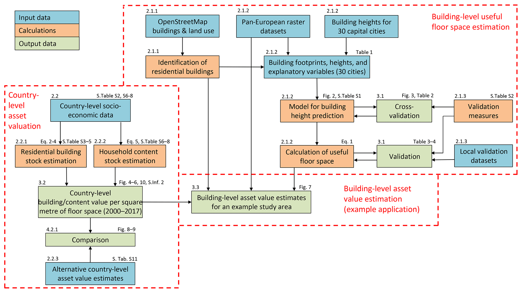
Figure 1Workflow of the study. Boxes are coloured according to categories explained in the legend. In the top left corners of the boxes are references to relevant sections of this paper. In the top right corners of the boxes are references to figures, tables, supplementary tables (S.Tab.) in Supplementary Information 1, equations, and Supplementary Information 2 (S.Inf. 2).
2.1 Building-level useful floor space estimation
2.1.1 Identification of residential buildings
Applying a building-level damage model requires information on the analysed objects such as size and value. Before those quantities could be calculated, residential buildings have to be identified in the area of interest. A variety of cartographic sources could be used depending on local availability, from governmental databases to topographic maps and remote sensing. The problem of accurately identifying buildings and occupancy, especially with open data, is outside the scope of this paper as this issue is still subject to intense research (Schorlemmer et al., 2017). Here, we use OpenStreetMap (OSM), which is an openly available, crowdsourced online database of objects constituting the natural and artificial environment of the Earth's surface (OpenStreetMap, 2019). Though created primarily by volunteers, it also contains spatial data imported from governmental GIS databases for some cities, regions, or even whole countries (e.g. resulting in exceptionally comprehensive data on buildings in the Netherlands). In the context of this study the data of interest are buildings represented in a vector layer of building footprints. Occupation of buildings (residential and other) is not always indicated but can be further identified using land use information also contained in OSM.
We obtained the OSM building and land use layers to develop the building size estimation method. The download was carried out during 22–25 January 2019 through Overpass API, a system that allows us to obtain custom selections of OSM data (OpenStreetMap Wiki, 2019). The data obtained included two map features (buildings and landuse). For the purpose of this analysis, residential buildings were objects from the buildings layer which (1) had the tags “residential”, “apartments”, “house”, “detached”, or “terrace” and (2) had the tag “yes” (which indicates that a building exists, but its function is not defined) and were located within an object from the landuse layer which was tagged as residential. Data retrieval and processing into other GIS formats was done with open-source solutions, namely Python with GDAL/OGR tools.
2.1.2 Building size estimation
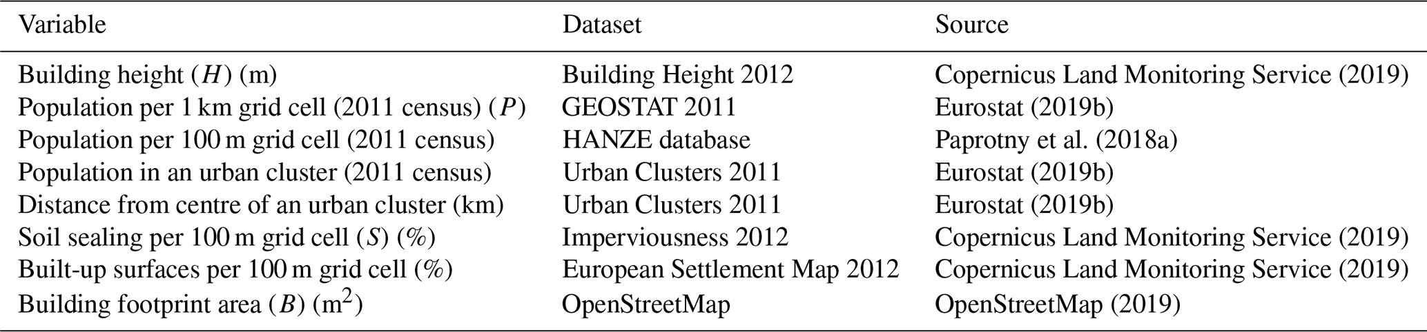
Once residential buildings, i.e. their footprints, are obtained, their size in terms of usable floor space area needs to be derived. The usable (also called useful) floor area of a dwelling is the total area of the rooms, kitchen, foyers, bathrooms, and all other spaces within the dwelling's outer walls. Cellars, uninhabitable attics, and, in multiple-occupancy houses, common areas are excluded (OECD, 2019; Statistics Poland, 2019). This information is not directly available; it can be indirectly estimated from building height or the number of floors. Yet, those variables are very rarely recorded in OSM and typically not accessible from other sources either. A method of estimating building height and consequently the number of floors of a building from publicly available datasets was therefore devised here, so that the floor space area could be computed as a product of building footprint area and the number of floors. A predictive model was created by building a Bayesian network (BN) correlating the variable of interest – building height – with seven candidate variables obtained from OSM and pan-European spatial datasets (Table 1).
Copernicus Land Monitoring Service (2019)Eurostat (2019b)Paprotny et al. (2018a)Eurostat (2019b)Eurostat (2019b)Copernicus Land Monitoring Service (2019)Copernicus Land Monitoring Service (2019)OpenStreetMap (2019)Table 1Variables considered for the building height prediction model. Abbreviations are shown for variables included in the final model (Fig. 2).
A Bayesian network is a graphical, probabilistic model which allows multivariate dependency analysis and provides uncertainty distributions of the predictions made with it. BNs are directed acyclic graphs consisting of nodes (representing random variables) and arcs indicating the dependency structure (Hanea et al., 2006). Here, we use a class of BNs known as a non-parametric Bayesian network which are quantified with empirical margins and normal (Gaussian) copulas as a dependency model. The copulas are parametrized using Spearman's (conditional) rank correlation coefficient. This class of BNs is for continuous variables only. For the purpose of this study, we use our own implementation of non-parametric Bayesian networks as a MATLAB code, the mathematics of which are described in Hanea et al. (2015).
Building height was derived from a high-resolution digital surface model “Building Height 2012” by the Copernicus Land Monitoring Service (2019), which is available for 30 European cities (all European Union members' capitals plus Oslo and Reykjavik). Residential buildings (as defined in Sect. 2.1.1) for each location were extracted, totalling 2 375 058 records. For higher efficiency of the statistical analysis, a random 10 % sample was drawn to reduce to the size of the dataset. The sample contains 237 361 records, with the number of data points ranging from 123 for Valletta to 25 526 for Berlin. Variables for the model were chosen first based on the unconditional rank correlation matrix (Table S1 in the Supplement) and then analysing the (conditional) rank correlations between variables.
The final model is presented in Fig. 2. Building height (H) has the highest rank correlation (0.47) with population density per 1 km grid (P). Among the remaining six variables, the highest conditional rank correlation with H was recorded for building footprint area (B). Soil sealing (or imperviousness) per 100 m grid cell (S) had the highest conditional rank correlation with H among the remaining five variables. Further variables had only very low (r<0.05) conditional correlation with H; therefore only three variables were used to explain H. The remaining arc between P and S was added due to high correlation between the two. B and S were not correlated ().

Figure 2A Bayesian network for predicting residential building height. Values on the arcs represent the (conditional) rank correlation; values under the histograms showing the probability density function are the mean and standard deviation of the marginal distributions, with density on the y axis and minimum–maximum values on the x axis. H – building height (m); P – population density (persons km−2); S – soil sealing (%); B – building footprint area (m2). Graph generated using Uninet software (Hanea et al., 2015).
The dependencies defined in the model can be explained theoretically as follows. Firstly, high population density was highly correlated with height, as one might expect the presence of tall residential buildings (high-rises, tower blocks) in densely populated cities. High buildings also typically have a large footprint compared to single-family houses. Finally, the height of buildings is correlated with soil sealing, as urban districts with apartment blocks are largely covered by artificial surfaces providing supporting services to the buildings, such as roads, sidewalks, parking lots, etc. Such surfaces reduce the perviousness of the soil. On the other hand, small single-family houses are rather found in less-densely built-up and populated suburban zones.
The accuracy of the model is analysed in Sect. 3.1. Predicted building height was transformed into floor space area F using the following empirical formula:
where H is the building height in metres and B is the building footprint area (m2); a, b, and c are empirical coefficients. The ⌊⌋ function indicates rounding down the value in brackets to the nearest integer. The empirical parameters were set to a=2.4 m, b=3.3 m, and c=70 %. This indicates that the average height of floors was assumed to be 2.4 m, except the first floor (b). This value was first based on Figueiredo and Martina (2016), who analysed building sizes in Italy, and then adjusted using the comparison between observed and predicted (using methodology described herein) number of floors in the validation case study of houses in the Polish coastal zone. The lowest storey includes the flood elevation above ground, which was found to be 90 cm on average for German households affected by floods between 2002 and 2014. Consequently, m. Equation (1) further includes an allowance for the fact that not all floor space of a building is useful, as it can contain common spaces or other uninhabitable spaces. Such unusable spaces are assumed to be 30 % of total floor space, leaving 70 % as useful space (c). These values were based on the comparison between observed and predicted (using methodology described herein) usable floor space of validation case studies of flood-affected houses in Germany and the Netherlands (see Sects. 2.1.3 and 3.1).
The described routine can be applied to any location in Europe for which at least the building footprint area is known. The Bayesian network model can be used when data for any variable are missing, though the building footprint is required for Eq. (1). In fact, all data should be available at least for the European Union countries: building footprint from OSM or other databases and soil sealing/gridded population from pan-European datasets. An example application of the model to exposure computation is shown in Sect. 3.3.
2.1.3 Validation of the method
Predictions of building height, number of floors, and floor space area are compared with observations using several error metrics (Moriasi et al., 2007; Wagenaar et al., 2018):
-
Pearson's coefficient of determination (R2) was used to measure the degree of collinearity between predicted and observed values, with higher R2 indicating stronger correlation.
-
Mean absolute error (MAE) was used to measure the average absolute difference between predicted and observed values, with higher MAE indicating higher error.
-
Mean bias error (MBE) was used to measure the average difference between predicted and observed values, with positive MBE indicating overprediction and negative MBE indicating underprediction.
-
Symmetric mean absolute percentage error (SMAPE) normalizes MAE by considering the absolute values of predictions and observations, with a value close to 0 indicating a small error compared to the variability of the phenomena in question.
-
Root-mean-square error (RMSE) was used to measure the difference between predicted and observed values, with a higher RMSE indicating higher error.
Equations for the listed measures are shown in Table S2. For validation purposes, we use the predictions as mean (expected) values of the uncertainty distribution of the variables of interest per data point (building). We also analyse the uncertainty of the height prediction model and perform an out-of-sample validation.
An out-of-sample validation of building heights was done individually for each of the 30 capital cities contained in the sample quantifying the BN. Validation for all cities collectively was performed using 10-fold cross-validation. Predictions of building heights transformed into the number of floors were validated using a large (N=62 580) sample of residential buildings that were identified as potentially endangered by coastal floods and sea level rise in Poland according to a study by Paprotny and Terefenko (2017). The dataset contains building polygons with the number of floors and constitutes part of the Topographical Objects Database (BDOT) maintained by the office of the surveyor general in Poland. It was created through a combination of remote sensing, field surveys, and administrative registers and is accurate as of the year 2013. The quality of the data should correspond to a 1 : 10 000 scale map, and the quantitative information contained in the dataset should nominally deviate from real values by no more than 20 %. For each building, the footprint area, population, and soil sealing were derived to run the BN-based model and converted into number of floors using Eq. (1).
Validation of floor space area predictions was carried out using results of post-disaster household surveys covering six river floods and three flash floods that affected Germany between 2002 and 2014 and a river flood along the river Meuse in the Netherlands in 1993 (Thieken et al., 2005, 2017; Rözer et al., 2016; Spekkers et al., 2017; Wagenaar et al., 2017, 2018). In the German surveys, conducted mostly in the south and east of the country, respondents were asked to provide information on the floor spaces of their households. The floor space area of multi-family buildings was extrapolated using the total number of flats in the building multiplied by the floor space of the surveyed household. In the Dutch survey, the information on the floor space area was taken from the national cadastre. For each survey data point an OSM building polygon was downloaded and other statistics necessary to run the BN model were extracted. However, both survey datasets include considerable uncertainty related to the location of individual buildings. Therefore, the analysis was done only for buildings for which there was good confidence that corresponding OpenStreetMap buildings were correctly identified, based on the building footprint area recorded in the survey datasets. Also, the analysis for Dutch data was done only for single-family houses, as the floor space data for apartment buildings only referred to particular households, not the whole buildings. As this was also occasionally the case in the German sample, instances of floor space being less than half of building footprint were excluded. This threshold also helps excluding residential buildings with large non-residential parts (e.g. agricultural or commercial), as was done by Fuchs et al. (2015).
2.2 Country-level valuation of buildings and household contents
When the floor space of a building is known, it is multiplied by the average replacement cost of dwellings and household contents per square metre. The total floor space of dwellings in a country is available for European countries due to recording of this information in population and housing censuses, sometimes also in household surveys (Eurostat, 2019a). This data has to be gathered from national statistical institutes, as it is not collected by Eurostat. Some countries only disseminate floor space information at census dates (e.g. Italy, Portugal, Spain), while others carry out surveys less frequently than annually (e.g. France) or only as part of the EU Survey of Income and Living Conditions (e.g. Norway, Sweden). There are also countries that calculate continuous balances of housing stock or extract data from housing registers, thus providing annual time series of floor space area in the country (e.g. Denmark, Germany, the Netherlands, Poland, Romania). Finally, for some countries only household floor space data from the 2012 edition of the EU Survey of Income and Living Conditions were available (e.g. Belgium, Norway, Sweden). Information on the data collected on dwelling stock is provided in Table S3.
2.2.1 Residential buildings
Statistical institutes in most European countries are recording the stock of fixed assets, including dwellings, for purposes of national accounting (Eurostat, 2013). Annual time series of the gross stock of dwellings are available for 22 EU countries from Eurostat, though the data for two countries – Latvia and Poland – could not be used due to major methodological differences which are discussed in Table S3. The value of dwellings is provided from the aforementioned resource in nominal and the previous year's prices. A deflator to obtain real (2015) prices was constructed based on the two time series. Finally, the value of all dwellings was divided by the total floor space area in a country to obtain average value per square metre. The method does not consider building types or quality, but this information is scarcely available from open datasets on buildings. Information on specific data sources on dwelling values is provided in Table S3.
The remaining EU countries and three other western European nations (Iceland, Norway, Switzerland) required more data collection efforts. According to the European System of Accounts (ESA) 2010 manual (Eurostat, 2013), the perpetual inventory method (PIM) should be applied whenever direct information on the stock of fixed assets is missing. In practice, most countries use PIM to arrive at the stock estimates that are published through Eurostat (Eurostat and OECD, 2014). PIM accumulates past investments over time to indirectly estimate the value of the stock (U.S. Department of Commerce Bureau of Economic Analysis, 2003). The general formula for PIM to obtain the gross stock is as follows (National Bank of Belgium, 2014):
where S denotes stock of an asset, t is the calendar year, j is an annual increment, I is investment in year t−j, L is the maximum service life of an asset in years, and G is the proportion of an asset purchased in t−j and still in use in t.
Three quantities are needed to obtain the stock of dwellings S: investment in housing, an estimate of the dwellings' service life, and the fraction of dwellings of the same vintage that are retired every year. Investment (gross fixed capital formation for asset type “dwellings”) is available from Eurostat, national statistical institutes, or country-specific research estimates. However, sufficiently long investment series were only identified for Sweden, while for other countries they had to be extrapolated using total investment or gross domestic product (GDP), a method which is also applied by national statistical institutes when necessary (Eurostat and OECD, 2014; Rudolf and Zurlinden, 2009).
Parameters L and G are assumptions that usually stem from estimates of average service life of assets. Most national statistical institutes derive G by assuming certain probability distributions known as retirement patterns or survival functions. This means that a different proportion of dwellings is retired each year, with the highest proportion around the average service life. However, this requires assuming a certain probability distribution, and national methodologies indicate a large variety of those (normal, log-normal, gamma, Weibull, Winfrey, etc.). Further assumptions have to be made regarding the distribution's dispersion and maximum service life (OECD, 2009). It also vastly increases the length of investment time series necessary to apply PIM, which would require collecting investment series going back even to the early 19th century. In effect, some countries with short data series apply no survival function (Eurostat and OECD, 2014). This approach is known as “simultaneous exit” and assumes that all assets are only retired when reaching a given service life. Equation (2) is therefore simplified to
which now only requires the assumption of an average service life of dwellings Lmean. As a sensitivity check, we applied log-normally and normally distributed retirement patterns to the Swedish investment series, the longest we have collected. We assumed a dispersion factor from 2 to 4 (i.e. ratio of mean and standard deviation of service life) and maximum service life equal to twice the average, as suggested by the National Bank of Belgium (2014). The calculation yielded a gross stock of dwellings in Sweden in 2017 lower by 5 %–15 % compared to an estimate derived with no survival function. Consequently, we relied on the simplified method to apply PIM for six countries (Iceland, Malta, Norway, Spain, Sweden, and Switzerland). Lmean for each country was taken from national methodologies collected in a survey by Eurostat and OECD (2014), except for Switzerland, which was taken from Bundesamt für Statistik (2006).
For a further four countries, where data on investment are limited, but the balances of the number of buildings and their floor space are available, a modified PIM was applied. In those cases, we computed an initial estimate of the stock of dwellings (Bulgaria in 1999, Latvia in 2000, Poland and Romania in 1995) based on national construction costs in the base year, and then we used annual data on investments in, and retirement of, dwellings in the country to arrive at a time series of the gross stock. In this case Eq. (2) becomes
Here Gt is the fraction of the stock retired during year t. In this way, service life assumption and long data series are not needed, with the drawback of assuming uniformity of the existing stock of dwellings and that all investment goes into building new dwellings rather than also into renovation of dwellings. We also tested the method from Eq. (4) using extrapolated investment series, but it yielded far lower estimates of building asset values which were also much lower than for neighbouring central European countries. With a modified PIM, the exposure estimates were more closely aligned to countries at a similar level of development. Calculation for the remaining country, Croatia, was not possible due to the lack of even basic data needed for the computation. Data sources and assumptions for individual countries are provided in Tables S3 and S4, while the overall reference to methods used is given in Table S5.
2.2.2 Household contents
Data availability for the stock of household contents is much lower than for dwellings. This item is termed in national accounting “consumer durables” and assumed to be consumed within the accounting period, rather than accumulated, as those durables are not relevant from the perspective of economic production processes. As such, they are considered memorandum items in ESA 2010 (Eurostat, 2013), and consequently few European countries have published national estimates of the stock of consumer durables, namely Estonia, Germany, Italy, and the Netherlands (OECD, 2019). Yet, even those few available datasets include personal vehicles in the stock. Cars and motorcycles are typically located outside the residential buildings; hence including them in estimates disaggregated by square metre of floor space would not be suitable. Further, they are insured separately from houses and their contents and therefore not included, for example, in reported flood damages from post-disaster household surveys (Thieken et al., 2005; Carisi et al., 2018; Wagenaar et al., 2018). Given all those constraints, we calculate our own estimates of the stock of household contents (durables) for all countries included in the study.
In order to estimate the stock of household contents, the PIM method is applied again. However, the contents consist of various durables of different service lives; therefore Eq. (3) has to be rewritten as
where the stock of household contents equals the sum of stocks for items , each with service life La. No retirement pattern was assumed; hence all items are included in the stock until reaching their average service life. The data on annual investment were gathered from final consumption expenditure of households split according to the Classification of Individual Consumption by Purpose (COICOP). The relevant durables are a set of 12 items at the COICOP four-digit level, i.e. all durables except for items under code 07.1 “Purchase of vehicles”. However, only Sweden publishes annual data with such level of detail; data disaggregated at the COICOP three-digit level are disseminated for 28 countries, at the COICOP two-digit level for Switzerland, and no data are available for Croatia. We therefore computed the average share of spending on durables within the COICOP three-digit categories using 5-yearly household survey data from Eurostat on detailed consumption expenditure patterns per country. The same approach was previously applied by Jalava and Kavonius (2009) to estimate the stock of durables in Europe. It allowed us to estimate spending on durables from COICOP three-digit data. Assumptions about service life of durable items (aggregated to COICOP three-digit items) were calculated from German estimates presented by Schmalwasser et al. (2011). We averaged 1991 and 2009 estimates of service lives from that study and weighted the COICOP four-digit items according to their share in spending. The service life of appliances for personal care (COICOP code 12.1.2) was not provided in the aforementioned resource; hence it was taken from Jalava and Kavonius (2009). A list of durable items, assumptions on their service life, and the share of spending on durables per COICOP three-digit item are shown in Tables S6 and S7. For Iceland detailed consumption expenditure surveys are not available; hence the average share in 15 EU members states was used instead.
Final consumption expenditure data were collected from Eurostat, OECD, and national statistical institutes. Due to the very long estimated service life of durables in the “personal effects” (COICOP code 12.3.1) category (45 years), the spending on those items had to be extrapolated using data on total private consumption expenditure, or GDP. This should have, however, limited influence on the results for recent years given the rather small share of spending on durable personal effects. For France, which has detailed expenditure going back to 1959, truncating the data to 1995 (the minimum availability for the countries considered except Malta) and extrapolating them with total private consumption resulted in a 2 %–5 % lower estimate of the stock of household contents, depending on the year. The uncertainty increases when moving back in time. Detailed sources of data are shown in Table S8. The calculation in Eq. (5) was carried out with expenditure time series in real (2015) prices and then converted to nominal prices using country- and item-specific deflators. Additionally, country-specific deflators of household contents were devised from the time series of the stock of consumer durables in real and nominal prices. Those deflators can be used to estimate the value of damages to household contents in real prices. Lastly, the stock of consumer durables was divided by the total floor space area in a country to obtain average value per square metre, as for residential buildings. However, for several countries, due to a large number of unoccupied dwellings (as identified in data from Eurostat, 2019a), only the floor space area of occupied dwellings or the number of households was used in this calculation. Instances of using different floor space area estimates to obtain average building and content values are indicated in Table S3.
2.2.3 Validation of the method
Estimates of building and content value cannot be directly validated due to the lack of information on this subject at the level of individual objects. We can only compare our results with other published results, which is done in Sect. 4.2.1. Those published results include two pan-European studies: (1) a flood risk assessment for the European Commission – Joint Research Centre (JRC) by Huizinga et al. (2017) and a (2) seismic risk assessment for the “Network of European Research Infrastructures for Earthquake Risk Assessment and Mitigation” (NERA) project by Ozcebe et al. (2014). Both studies used construction cost surveys and manuals as well as regression analyses with socio-economic factors. Additionally, we compare estimates calculated in this study with values used in available local or national risk assessments.
3.1 Validation of building height and floor space predictions
The exposure estimation procedure was first validated by comparing observed and modelled residential building height. This analysis was done through a 10-fold cross-validation using a 10 % sample of residential buildings in 30 European capitals (Sect. 2.1.2). Figure 3 displays a comparison between observed and modelled heights. The coefficient of determination (R2) is a moderate 0.35. Still, the model correctly predicts the average height (9.69 m versus 9.60 m observed) but underestimates the variation, as the modelled sample has a standard deviation of 3.30 m versus 5.89 m found in observations. In effect, despite the low bias of the model in general, the height of tall buildings (more than 20 m high) is mostly underestimated. Mean absolute error is 3.25 m, which is 34 % of the mean height (Table 2).
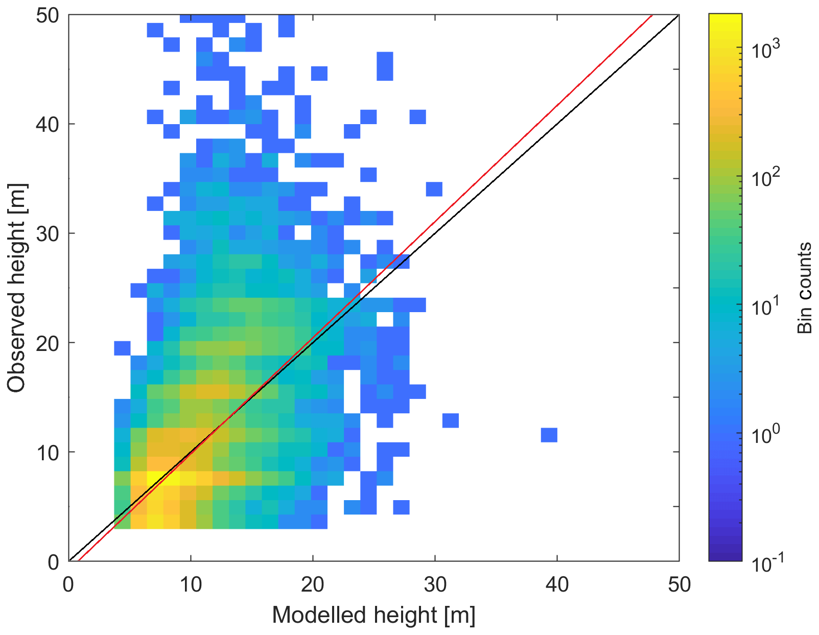
Figure 3Binned scatter plot for observed and modelled heights of residential buildings for 30 European capitals, out-of-sample validation. The black line is the 1 : 1 line, and the red line is the linear regression line.
Table 2Validation statistics for the building height prediction model (mean value of the uncertainty distribution) for different cities. For all cities, the results are an average of results for a 10-fold cross-validation. For individual cities, the results are an out-of-sample validation (i.e. the model's sample excluded the city that was validated).
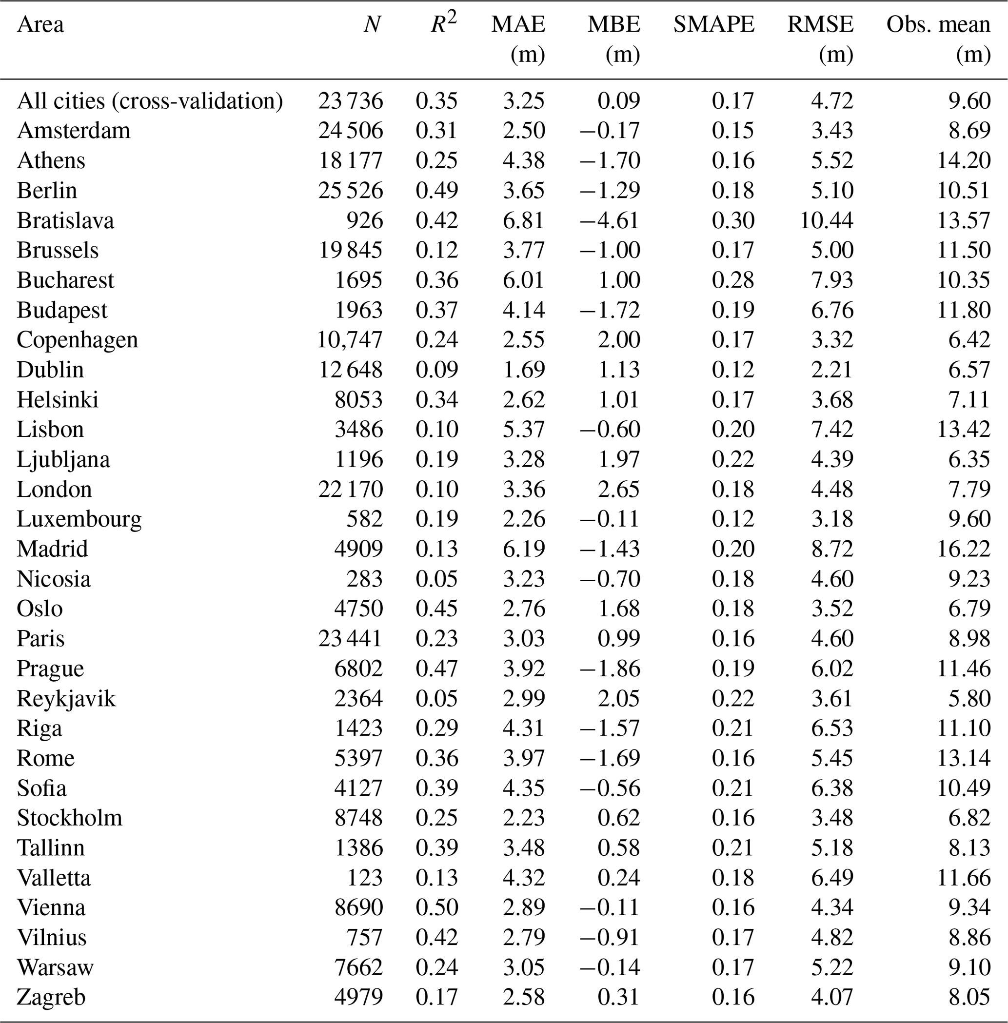
An out-of-sample validation was also carried out for each city in the dataset, where the validated capital was left out from the data quantifying the dependency structure of the BN model (Table 2). The lowest R2 values were computed for Nicosia and Reykjavik (0.05), though the latter has the lowest average building height among the cities considered here. On the other end of the scale are Vienna (0.50) and Berlin (0.49). Relatively low errors and bias was found for Amsterdam, Luxembourg, Stockholm, Vienna, Warsaw, and Zagreb, for example. The largest MAE and negative MBE were identified for Bratislava (6.81 and −4.61 m, respectively), while the highest MBE was recorded for London (+2.65 m).
Table 3Validation statistics for the building height prediction model (mean value of the uncertainty distribution) for various sets of residential buildings.
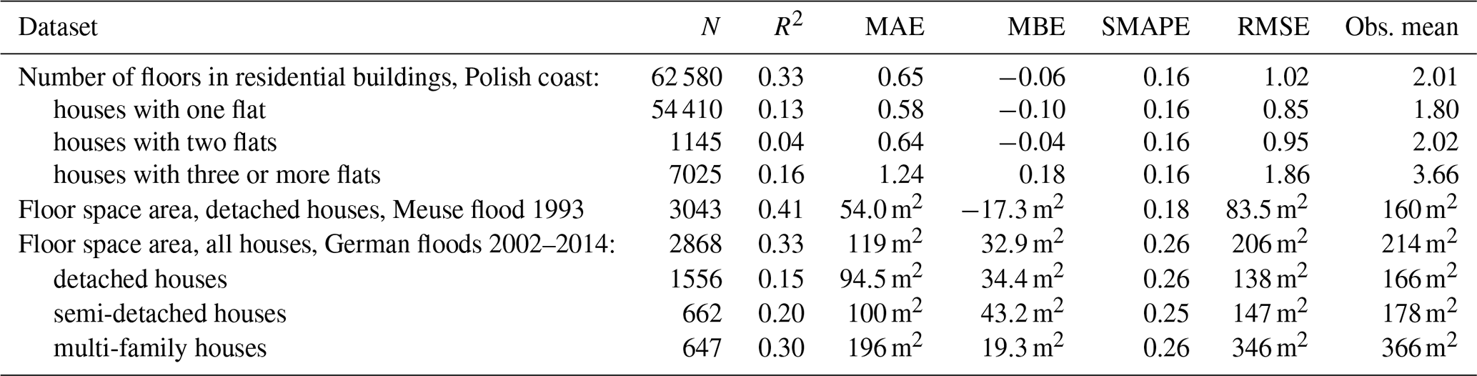
Table 4Hit rate of predictions of the number of floors for Polish residential buildings at risk of sea level rise and coastal floods. Bold font indicates the percentage of the correctly predicted number of floors.
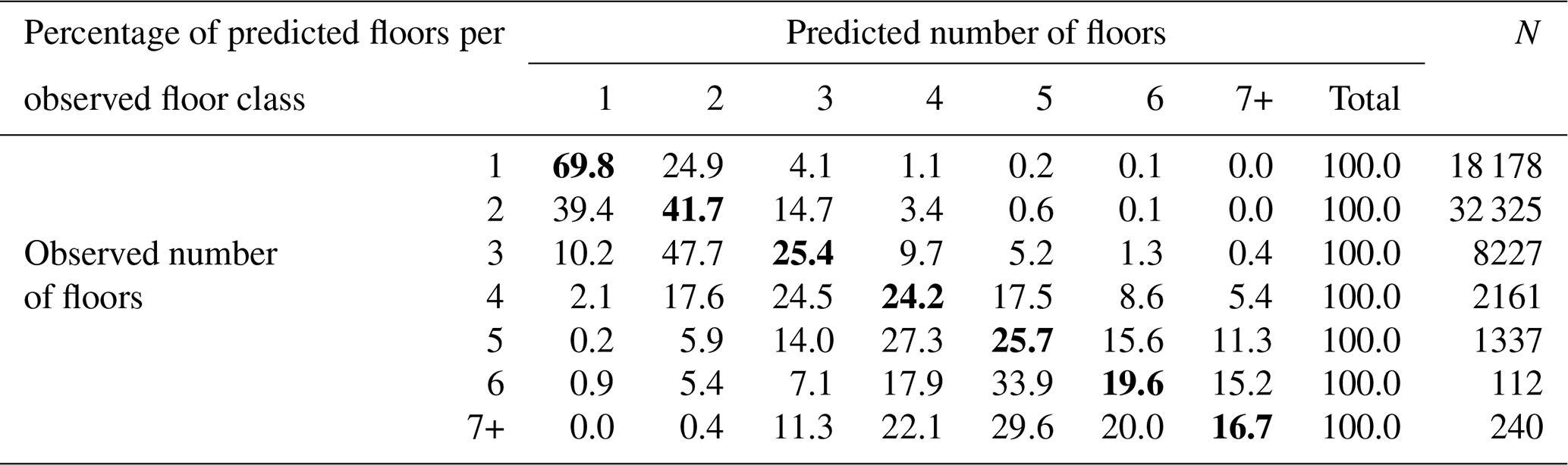
The second step in obtaining floor space – the number of floors – was tested against a large number of Polish residential buildings located in the coastal zone, obtained from the national database BDOT. Results in Table 3 show that average error is slightly less than a third of the average number of floors. R2 for particular building types is low, but better overall, as the method clearly has the ability to distinguish small single-family houses from multi-family buildings. Overall, 45.0 % of the buildings had the number of floors predicted correctly (Table 4). The number of floors is rather underestimated than overestimated, especially for higher buildings. The error does not exceed one floor for four to six floor buildings in almost 70 % of cases. For buildings with seven floors or more, underestimation is mostly by two floors.
Finally, predictions of the floor space area were tested against Dutch and German households (Table 3). The average error was equal to about a third of the average building height of the Dutch buildings. For the German buildings, average error was almost half the average height. The size of Dutch buildings is on average slightly underestimated (−11 %), but the opposite happens for German houses (+15 %). Nonetheless, the model can clearly distinguish between single-family (detached) and multi-family houses. Larger variation in heights of apartment buildings also results in higher R2 and lower SMAPE compared to detached houses which are typically quite similar in the number of floors. Mean absolute error (MAE) is still larger for multi-family houses, but bias is lower than for the other two types of buildings in the German sample.
3.2 Pan-European estimates of building and household content value
As described in Sect. 2.3, statistical data on buildings and household expenditure were collected for a study area of 30 countries (Iceland, Norway, Switzerland and the European Union except for Croatia). The dataset reveals a considerable stock of residential assets in place. Based on those statistical data alone, we estimate that there were 259 million dwellings in the study area at the end of 2017, some 12 % of which are vacant or occupied seasonally. Those dwellings had a collective useful floor space area of almost 24 billion m2 and were worth EUR 36.7 trillion in gross replacement costs. At the country level, the value of assets per square metre of floor space varies substantially (Figs. 4 and 5). Iceland had the highest estimated value of dwellings per square metre (EUR 2284), followed closely by Germany and Finland. Differences in dwelling sizes, vacancy rates, and average number of persons per household result in average home replacement costs varying even more. Icelandic dwellings, typically larger than the European average, are the most expensive in Europe, though in per capita terms costs are higher in Denmark (Fig. 4a). On the other side of the spectrum, Romanian dwellings are the smallest (in terms of average floor space) and cheapest to reconstruct (EUR 412 per square metre). Higher values are recorded in Bulgaria, Lithuania, and other central European states. Southern European and Benelux nations fall in the middle of the distribution (Fig. 5a). The stock of dwellings and their prices have grown rapidly since the year 2000 (Fig. 6a). Almost 5 billion m2 of floor space was added and the average dwelling size has increased as well. In nominal prices, the average replacement cost of residential buildings per square metre of floor space has grown at least by 14 % (Greece) and as much as 6-fold in Romania; the growth in average European dwelling costs was 53 %. In constant prices, the average replacement cost of the existing dwelling stock has declined in four countries (Denmark, France, Luxembourg, Slovenia). The highest growth of 79 % was recorded in Slovakia. The average European replacement costs per square metre have gone up by a modest 7 %. Changes of dwelling value in constant prices should be interpreted as change in the characteristics of the stock of residential buildings: its average quality, material, size, and type (single- and multi-family houses, dwellings for permanent or seasonal use, etc.). There appears to be no clear pattern of the distribution of those changes, but southern countries had rather lower rates of cost growth than the northern states. The country with the highest replacement costs per square metre changed multiple times in the 17-year timeframe, alternating between Germany, Ireland, Sweden, Switzerland, and finally Iceland.
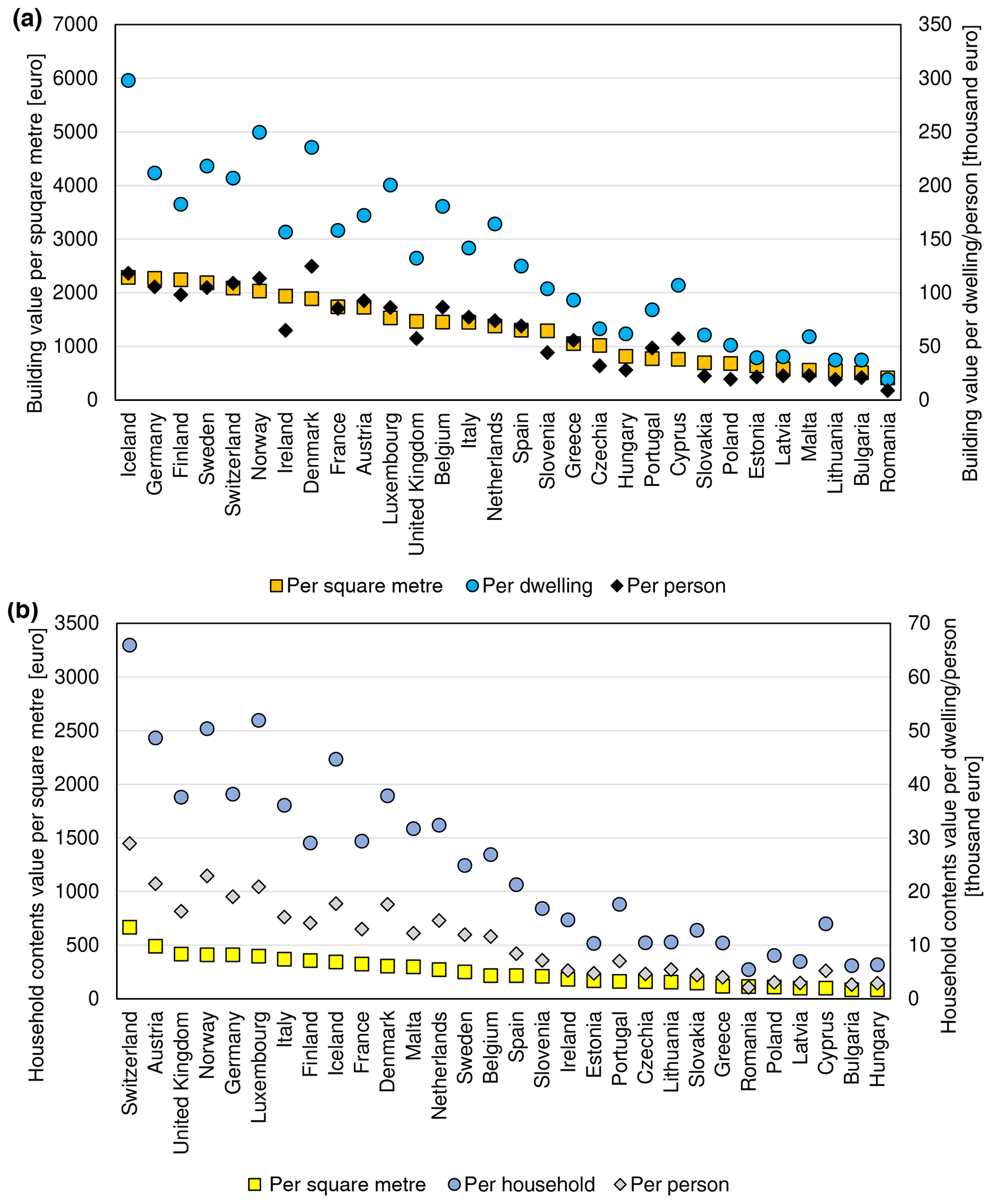
Figure 4Value of (a) residential buildings and (b) household contents per square metre of floor space, per dwelling/household and per person, ranked by values per square metre of floor space, as of 2017.
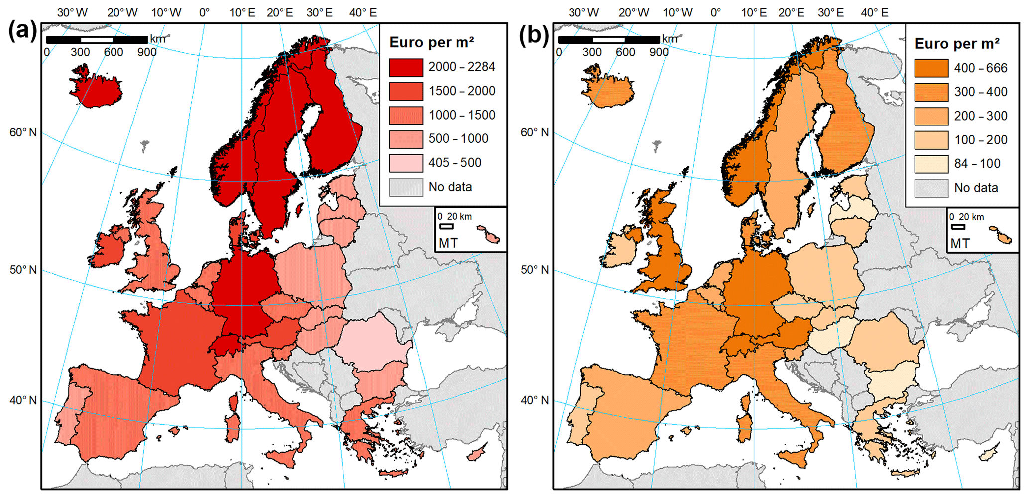
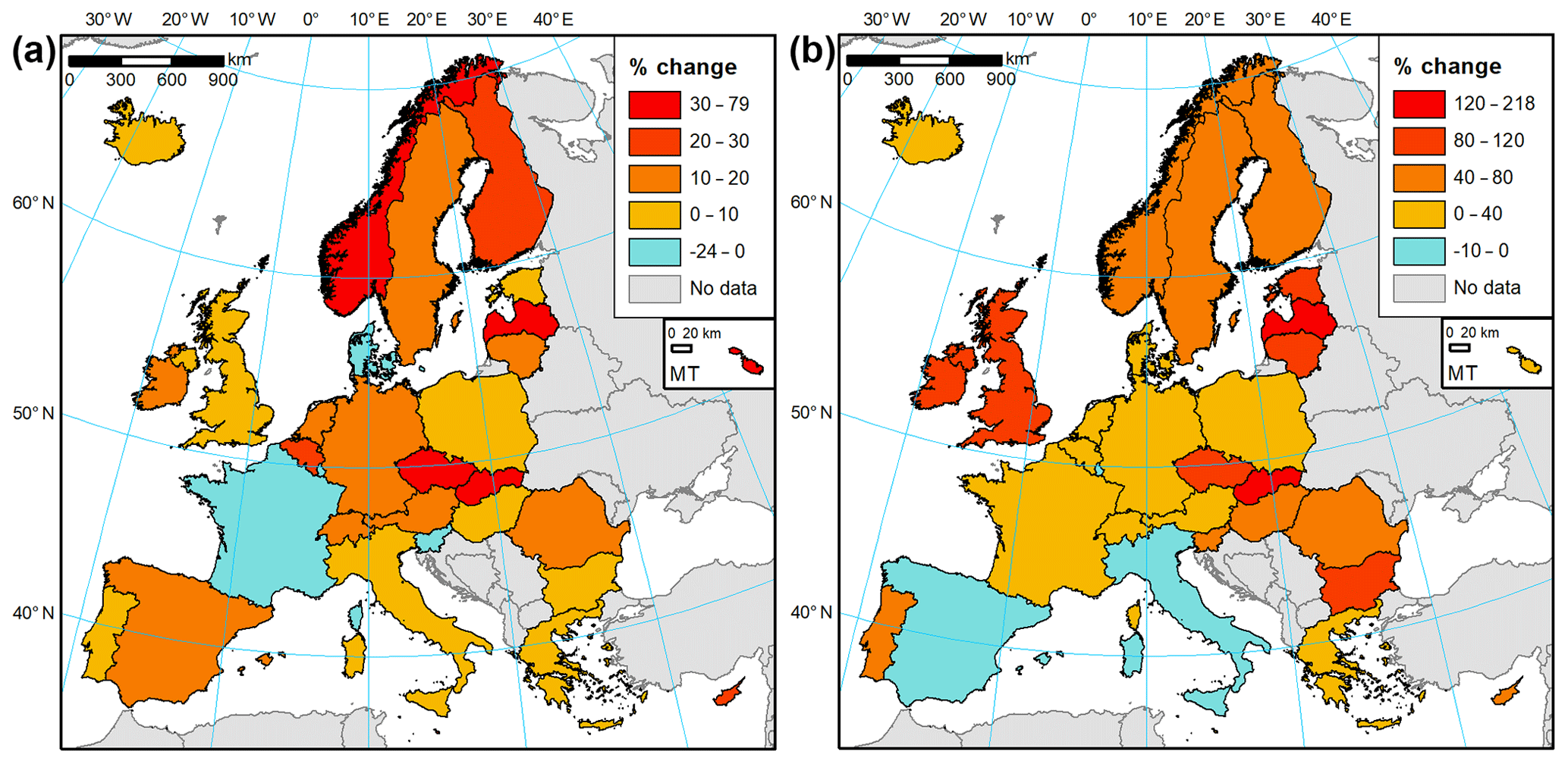
Household contents in Europe are a diversified collection of durable items, which we estimated were worth EUR 6.6 trillion at the end of 2017. Furniture, furnishings, and floor coverings constituted 39 % of the gross stock of household contents, followed by jewellery, clocks, and watches (25 %); audiovisual, photographic, and information processing equipment (11 %); major household appliances (10 %); and various other tools, equipment, and appliances (16 %). Variation between countries is higher than for dwellings (Fig. 5b), albeit mainly due to exceptionally large stock of consumer durables in Switzerland (EUR 666 per square metre as of 2017). Nordic countries are less prominently featured in the top of the ranking compared to building values (Fig. 6b). The highest values are recorded, apart from Switzerland, in Austria, the United Kingdom, Norway, and Germany. Switzerland also comes first in the value of contents per household and per person. The lowest stocks of durables per square metre were estimated for Hungary (EUR 84), Bulgaria, and Cyprus, though Cyprus's value is a result of large sizes of dwellings; hence an average Cypriot household has more assets than homes in other central European countries. In nominal terms, the growth in household contents was smaller than for dwellings in nominal terms: 30 % for the growth in average European value per square metre, varying from decline in Ireland to an almost 4-fold increase in Slovakia and Romania. Yet, many household items have seen their prices grow slowly or decline, especially for electronic equipment. In effect, an average household in Europe had 19 % more consumer durables per square metre in 2017 than in 2000, even if growth was lowered by the increase in average floor space available to households. Three countries (Italy, Luxembourg, Spain) recorded a decline (Fig. 6b), while a more than tripling of content value was recorded in Latvia and Slovakia. Growth was clearly higher in northern and central Europe than in southern Europe, as consumer spending on durables is very sensitive to the countries' economic performance. Switzerland had the highest values of contents per square metre throughout 2000–2017, while the lowest values were first estimated for Latvia, later Bulgaria, and finally Hungary.
3.3 Example application
To illustrate an application of the two components of the study – building-level height predictions and country-level valuations of residential assets – we downloaded current (as of 18 July 2019) OSM building data for Szczecin, Poland. This city of slightly more than 400 000 people is endangered in its low-lying parts by floods and sea level rise (Paprotny and Terefenko, 2017). OSM data indicated 27 971 residential buildings within the city limits. After calculating the footprint area of each building, corresponding population density and gridded soil sealing at 100 m resolution was extracted from pan-European datasets, as in Sect. 2.1.2. The BN model predicted building height for each building, which was then transformed into number of floors and consequently useful floor space area (Eq. 1). The average building was found to have a floor space of 467 m2 (uncertainty range 453–482 m2). The number of residential buildings and their average size were slightly larger than the values for 2017 recorded in the national statistics – 27 068 and 419 m2, respectively (Statistics Poland, 2019). The floor space of each building was multiplied by the average replacement costs of buildings and household contents in Poland in 2017, which is 683 and EUR 109 per square metre, respectively (Tables S3 and S7 in Supplementary Information 2). The total value of residential assets per building in a fragment of the city is presented in Fig. 7.

Figure 7Estimated residential asset values in a low-lying part of the city of Szczecin, Poland. Flood hazard zone from Paprotny and Terefenko (2017). Building geometry from © OpenStreetMap contributors 2019. Distributed under a Creative Commons BY-SA License.
Combining our exposure estimates with flood maps for extreme sea levels (Paprotny and Terefenko, 2017), we can identify 209 residential buildings in the city that exist within the 100-year flood hazard zone. Their aggregate value amounts to EUR 19.3 million. Then, a flood vulnerability model can be applied to estimate damages in case of the event, e.g. pan-European JRC depth–damage function for residential assets (Huizinga, 2007). This vulnerability model applied to water depths computed by Paprotny and Terefenko (2017) produces an estimate of damages from a 100-year flood event amounting to EUR 6.1 million.
4.1 Building-level useful floor space estimation
4.1.1 Uncertainties and limitations
Predictions of floor space area involve several uncertainties along the chain of computations. Firstly, the Bayesian network (BN) for predicting buildings was quantified based on a set of capital cities. Those cities vary enormously in size, cover 30 countries, and include at least to some extent the surrounding metropolitan area, but they do not include area of more rural character. Incorporation of those areas could improve predictions for single-family houses. At the moment, the R2 is lower for buildings located in local administrative units with a suburban or rural character, as identified by intersecting the available height data with the “Degrees of Urbanisation 2014” dataset by Eurostat (2019a). Yet, the mean absolute error is smaller and almost exactly proportional to the average building height at all three urbanization levels (Table S9).
Bias in predictions for high-rise buildings is observed, which can largely be a consequence of a relatively small number of those, even within large cities. Some errors originate in the source elevation model, which has a resolution of 10 m; therefore the height of buildings with small footprint areas could be less accurately assigned to OpenStreetMap polygons. Also, the validation information provided by Copernicus Land Monitoring Service (2019) shows variation in the accuracy of the elevation data between cities. Differences of 2–3 m are fairly common when compared with an alternative elevation model.
The OSM dataset is also not homogenous. Sometimes, individual buildings are not distinguished within a city block, creating an artificially large building, leading to overestimation of height in the BN model. The quality of building and land use is also uneven within the cities themselves, resulting in relatively few useful data points, e.g. for Nicosia, Rome, or Madrid. In the second step of obtaining floor space of buildings, i.e. calculating the number of floors, a constant height of each floor was assumed, though they tend to vary to some degree (Figueiredo and Martina, 2016). Also, a more diversified set of evidence could improve the calculation, similarly for the last step of deriving useful floor space, which depends on the assumption of what percentage of the area of a building is actually used for living purposes. This is particularly problematic with buildings of mixed use, as first floors of residential buildings are often utilized by shops and other services.
The method used for data analysis, a non-parametric BN, is a model configured primarily using expert knowledge. The dependency structure modelled with a Gaussian copula is the main assumption in the model that could affect the results. For comparative purposes of the height model's predictions, we also tested an ensemble learning method known as random forests (RF). It utilizes ensembles of regression trees, which split continuous variables into subsets in order to approximate nonlinear regression structures (Merz et al., 2013). We used the 10 % sample of the available data of building height and seven explanatory variables, the same as for the BN model, and we made a RF model with a 10-fold cross-validation. At each validation step, 100 trees were generated with a maximum of 50 leaves. For each split, one-third of the training data were used. The RF model produced slightly lower R2, higher RMSE, strongly negative MBE, and slightly lower MAE than the BN model. The performance was not far from the BN model (Table S10), though with more effort in tuning the various parameters of random forests a better result could be achieved.
4.1.2 Future outlook
Improving building height predictions for the purpose of exposure estimation would involve incorporating new sources of information. For building heights, lidar scanning results from smaller cities and rural areas should be incorporated to increase the diversity of the sample for a Bayesian network model. The model itself could also be built separately based on data of different typology (urban, suburban, rural) or for different parts of Europe. More diversified resources are needed as well to analyse the relationship between building height and the number of floors and the usable floor space of the building, which can differ between countries and building types. As a more immediate step, the code used in this study is expected to become publicly available to facilitate its application and further testing.
4.2 Country-level asset valuation
4.2.1 Comparison with alternative estimates
Estimates of residential building replacement cost per square metre from two external sources, by the JRC (Huizinga et al., 2017) and NERA project (Ozcebe et al., 2014) are gathered in Table S11 and compared with our estimates in Fig. 8. In a few cases, two different estimates are provided by the JRC, as two construction surveys were used as a source of information. Many of the JRC dwelling values for the year 2010 are similar to our calculation for the same year. In most cases, JRC provides higher estimates, which can be the result of using information on the construction costs of modern dwellings, rather than the replacement value of actually existing stock of housing. It is noticeable that the two alternative estimates by JRC differ substantially between themselves, especially for Germany and Poland, with our calculation falling in the middle of those two divergent cases. NERA project estimates (for year 2011) show much less variation between countries and almost uniformly show lower replacement costs for western European dwellings and higher replacement costs for central European houses. This is a result of using a set of “reference” countries and a regression based on GDP per capita. The latter was developed for global application, in effect compressing the variation in building costs: they vary only by a factor of 2 in the NERA estimates, despite GDP per capita in the countries in question changing by a factor of 15 as of the year 2011.
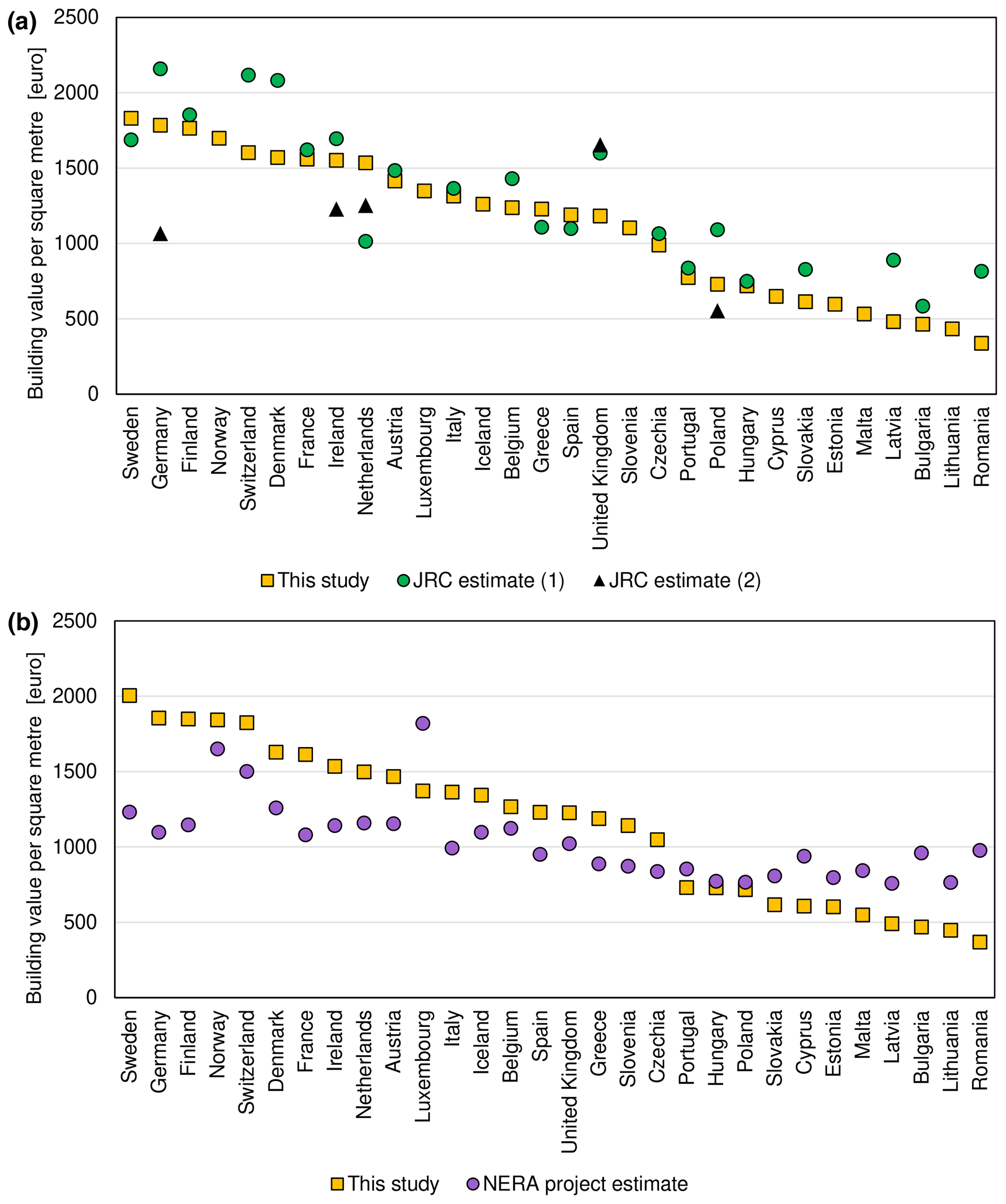
Figure 8Comparison of residential building values per square metre of floor space estimated in this study with (a) two estimates by the Joint Research Centre (Huizinga et al., 2017) for the year 2010 and (b) estimates from the NERA project (Ozcebe et al., 2014) for the year 2011.
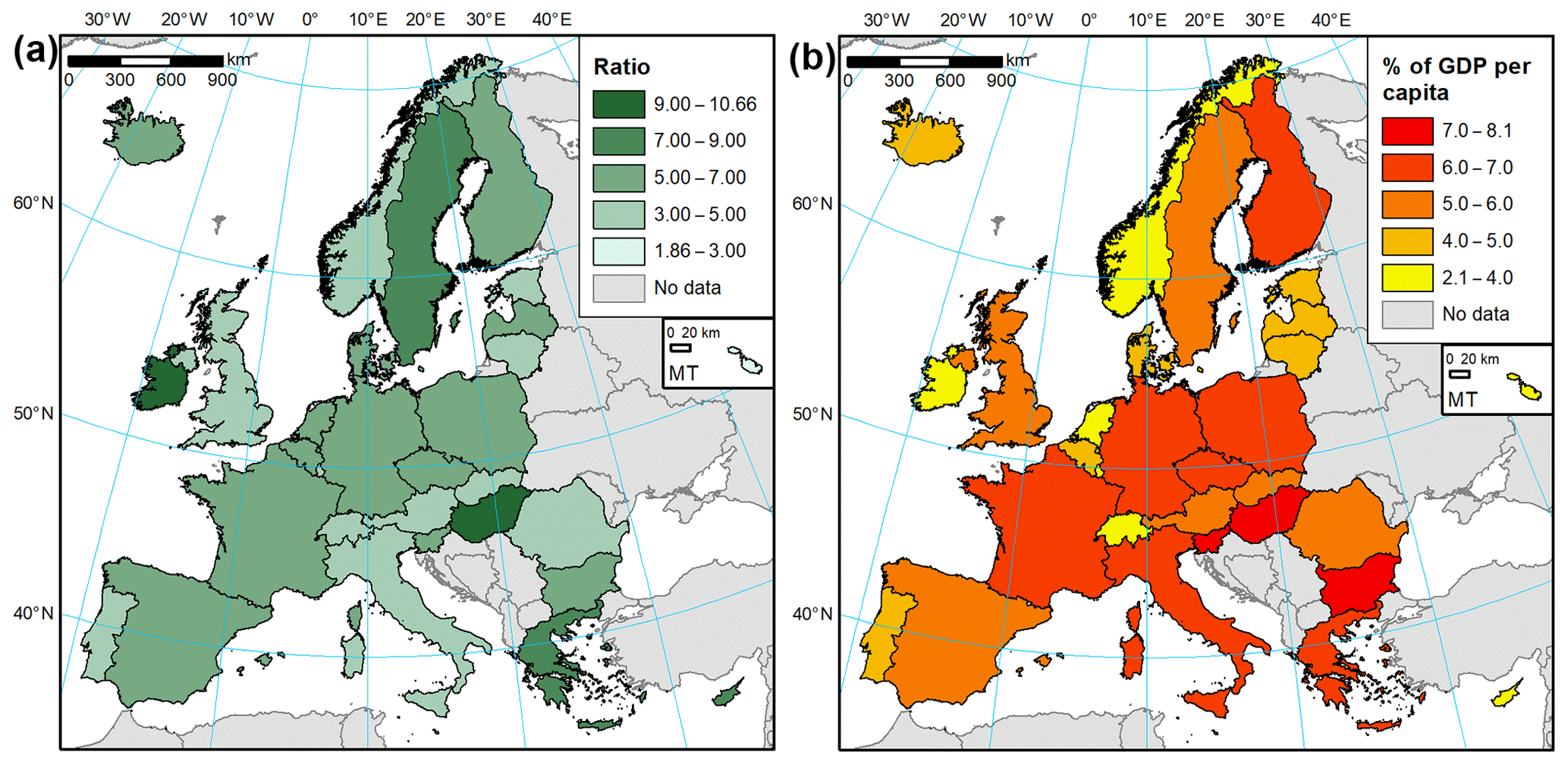
Household contents were not directly estimated by JRC in the study by Huizinga et al. (2017), but rather recommended taking half of the dwelling value. We therefore take 50 % of JRC's building value estimates for comparison with our estimates (Fig. 9). In all cases, the resulting household content value is much higher than our estimates. This could be partially a result of including more items in the contents, e.g. vehicles and semi-durables, though the extent of the term was not stated in the cited study. The 50 % also originate from the HAZUS model developed for the United States. In our study, a ratio close to 2 : 1 for buildings and contents was found only in Malta (1.86), while for other countries it is at least 3 : 1 (Fig. 10a). The average ratio is almost 5.7; therefore the resulting content value estimates are almost 3 times lower than those based on JRC building value estimates and a single building-to-contents ratio based on an American model.

Figure 9Comparison of household content values per square metre of floor space estimated for the year 2010 in this study with two estimates by the Joint Research Centre (Huizinga et al., 2017).
Some other literature estimated could be compared with our results. Studies based on German post-disaster surveys computed exposure based on an insurance sector guideline for residential building values deflated to a particular year with the construction price index (Thieken et al., 2005). Household contents were computed using a regression analysis of average insurance sums and local purchasing power. Average replacement costs of buildings affected by riverine floods between 2002 and 2013 were, on average, EUR 2594 per square metre in 2013 prices. The corresponding value for household contents was EUR 545, a ratio of 4.76 : 1. A weighted average of our estimates would be EUR 1944 and 377 at the price level of 2013. While both estimates are lower, the ratio of 5.16 : 1 is close to the value used in the German surveys. In a study of coastal floods and sea level rise in Poland (Paprotny and Terefenko, 2017), the authors used the average construction costs of new multi-family dwellings from the national statistical institute. Household contents were estimated on the basis of the average share of consumer durables in GDP identified for some developed countries by Piketty and Zucman (2014) and total floor space of dwellings in the country. Their estimates of EUR 936 and 147 for the year 2011 are higher than EUR 717 and 94 for dwellings and contents per square metre, respectively, computed in this study. However, the first value is based on new dwellings rather than replacement costs of existing stock, while the second value includes the cost of personal vehicles, which would add about half to our estimate of household contents (see Sect. 4.2.2), thus matching the other calculation. Silva et al. (2015) used residential building replacement costs from a governmental decree, updated annually, for their seismic risk assessment. As of 2013, the values per square metre separately for major cities, other urban areas, and rural areas were EUR 793, 693, and 628, respectively. Given the distribution of population by regional typology (Eurostat, 2019a), that amounts to around EUR 700 on average for the country, only slightly more than EUR 671 calculated here.
4.2.2 Uncertainties and limitations
Uncertainties related to economic valuations are largely methodological or related to limitations in the availability of some data for certain countries. Most of the gross stocks of dwellings are taken directly from national estimates, which are computed with a variety of assumptions related to service life and retirement patterns as well as investment data availability, coverage, and detail. As noted in Table S4, analysis of methods identified time series for two countries incomparable with others, but more datasets could be affected by local methodological specifics. The stock of household contents was computed with a uniform approach, but service life assumptions based on a German study might not be suitable for other countries. Also, the availability of historical data on consumption expenditure varies between countries and most detailed COICOP four-digit data are not accessible on a per-annum basis, necessitating assumptions about the share of durable spending in more aggregated data. Quality of the expenditure data could also be questioned given the very large differences between deflators for individual durable items between countries. This is most strongly visible in the data for Ireland, where prices of all items have dropped significantly since the year 2000 according to national statistics, which is not in line with the experience of other European economies. Consequently, the estimate of the stock of household contents for Ireland is likely too low and the strong upward trend is likely overestimated. Further, availability of dwelling and household numbers and especially the floor space statistics is not uniform. For some countries, data on temporal changes in average floor space per dwelling or the total area are not published. Yet, housing statistics are typically better for central European countries than western European states, quite the opposite to economic data availability. This is likely a result of poorer living conditions in the new EU member states prioritizing gathering information on the subject compared to western Europe, while their less-developed statistical systems usually generate lower detail and shorter time series of economic statistics.
The study presented only valuations of dwellings and household contents as gross stock, i.e. replacement cost without allowing for depreciation of assets. Merz et al. (2010) argued that for analysing damages to natural hazards net costs should be used instead, as the value actually lost is the remaining, depreciated value of assets. This is sensible in the perspective of national accounting, where changes to net stocks of assets are of main interest, e.g. for calculating GDP using the income approach or indicators such as net disposable income of households or net savings. Still, an asset typically cannot be restored to a particular depreciated state; therefore from the perspective of those who would need to pay for repair or replacement of the damaged or destroyed assets, the gross stock is a better indicator of the possible cost of post-disaster recovery. Depreciation of residential buildings varies to a large degree in Europe, not least due to very different assumptions on the patterns of depreciation. One method is called the “straight-line” method, as it assumes an asset loses a given percentage of its gross value each year and also requires definition of a retirement pattern as in the computation of gross stock. It is the default method in the ESA 2010 system and used in Belgium, France, Germany, Italy, Portugal, and the United Kingdom, for example (Eurostat, 2013; Eurostat and OECD, 2014). The other method, “geometric”, assumes that an asset loses a given percentage of its remaining (net) value and is used in Austria, Estonia, Norway, and Sweden, for example (Eurostat and OECD, 2014). The total stock of dwellings for the 22 countries available from Eurostat's database indicates a depreciation of 37 %, varying from 22 % in France to 55 % in Hungary (Eurostat, 2019a).
Consumer durables except for personal vehicles are used here for household contents on the basis of what items are actually insured and compensated after natural hazard events. Overall damages to households could be higher still. In the aftermath of the 2010 Xynthia storm, 8 % of flood-related insurance claims were related to cars on top of the 5 % of windstorm-related claims (FFSA/GEMA, 2011). In the study area, annual consumer spending on the purchase of vehicles amounts to some EUR 300 billion per year, 92 % of which is on motor cars (Eurostat, 2019a); hence assuming 11–12 years of service life (Schmalwasser et al., 2011) the stock of vehicles owned by households would amount to about half of the value of other consumer durables. Households also stock semi-durables and perishables. They are generally excluded from any assessments on household wealth due to the limited information on the usage time of items in question and their rather low value (Goldsmith, 1985). Spending on semi-durables (e.g. clothing, footwear, books, toys, small appliances) in the study exceeded EUR 750 billion in 2017; therefore it would add about 10 % to the estimated stock of durables for each year of assumed service life. Spending on perishables (e.g. food, fuel, medicines, newspapers) amounts to EUR 2.5 trillion per year in the countries considered here, but if households hold only a weekly stock of perishables, their total value is less than 1 % of the stock of durables.
4.2.3 Future outlook
Time series of building and content value provided in this study (Supplementary Information 2) have several applications. The main use is providing economic valuation of economic assets for natural hazard exposure and risk assessments carried out at the level of individual buildings (large-scale mapping). The time series could be used to correct past recorded damages from natural disasters for changes in asset reconstruction costs (separately for dwellings and contents) over time but also for changes in average quality of residential buildings and incomes of households that translate into more expensive consumer durables kept at home. Finally, the data could be used to rescale absolute damage functions, which generate damage estimates based on intensity of the hazardous event not as percentage of assets lost but as an absolute value for a given country in a specific year. In the field of flood risk, almost half of damage functions provide absolute values of damages instead of relative values (Gerl et al., 2016). With our data, for instance, flood damage curves for the United Kingdom at price levels of 2012 (Penning-Rowsell et al., 2013) could be applied to a German flood in 2002 by using the ratio of average replacement costs of residential assets in the UK and Germany in the respective years and currencies.
Further research on countries with good economic data would involve expanding the coverage in multiple aspects. Thematically, the net (depreciated) value of residential assets could be added to the dataset, as most of the necessary data have already been collected here. Net stock of dwellings is directly available for four more countries than the gross stock (Norway, Spain, Sweden, and Switzerland), while for others the PIM method would be used (Eurostat, 2013; Eurostat and OECD, 2014). Net stock of consumer durables can be computed from the same data as gross stock (Jalava and Kavonius, 2009). Estimates of the stock of vehicles (gross and net) could be added, disaggregated on a per-household or per-capita basis. Spatially, some developed non-European countries could be added which disseminate necessary data, e.g. through OECD. It should be possible to add Croatia and EU candidate countries to the dataset once they start publishing detailed EU-mandated national account data. In the temporal dimension, the dataset could be extended into the past, at least for certain countries with long data series (particularly France and the Nordic countries), so that it could be applicable to natural hazard case studies that occurred before the year 2000. An analysis of the trends in the stock of residential assets and economic factors determining it could possibly also provide insights into how could it change in the future, for the benefit of projections of natural hazard risk under climate change.
Furthermore, we provide valuations at the national level, which neglects possible differences between urban and rural areas as well between regions of countries. This is exemplified by the example of Portuguese asset valuations for urban, intermediate, and rural areas mentioned in Sect. 4.2.1. The possibility of regionalization of asset values could be investigated to capture the possible differences between regions of a country and urban/rural areas. Some countries have disseminated building stock data at a regional level (e.g. Germany, Poland, Spain), which could be combined with regional economic data such as GDP, gross fixed capital formation, compensation of employees in the construction sector, disposable income of households, etc. A statistical analysis on such a dataset could reveal determinants of regional variation in asset values. Also, these estimates could result in detailed dasymetric exposure mapping in Europe if combined with gridded population and land use datasets (Kleist et al., 2006; Thieken et al., 2006). Finally, incorporation of more detailed building characteristics, where available, could be applied to differentiate estimates of building value per square metre. Some countries distribute investment or stock data split by various types of buildings, which can also be incorporated into the PIM method. Several countries use different service life assumptions according to building type (Czechia, Estonia, Sweden), ownership (Latvia, Slovenia), age (Denmark, Germany), or material (some non-European countries), according to a survey by Eurostat and OECD (2014).
Still, most countries of the world do not disseminate such detailed housing, asset, investment, or expenditure data as were used in this study. Simplified methods to indirectly estimate exposure will therefore be needed. GDP per capita was incorporated by the NERA study as such a measure, but as the comparison in Sect. 4.2.1 has shown, this is not necessarily a good indicator. Also, there are significant variations between value of residential assets per square metre compared to GDP per capita and further differences between the composition of those assets. They vary by a factor of 4 and 6, respectively (Fig. 10b). The lowest exposure relative to GDP per capita is recorded particularly in countries where GDP is far higher than actual income of their population, like Ireland and Luxembourg. Using, for example, final consumption expenditure of households per capita as a proxy gives better results, reducing the variation in total residential assets per square metre between countries to a factor of 2.6. Estimates of this variable are available globally, for example, from the National Accounts Main Aggregates Database (United Nations, 2018). More detailed data are available approximately every 5 years from the International Comparison Programme, including household expenditure at the COICOP two-digit level. Developing such simplified approaches requires further analyses. Until then, we can propose the following rule of thumb based on the average asset values in the European countries: the total residential assets per square metre equal 6 % of GDP per capita, of which one-sixth are household contents.
In this study we have explored aspects related to estimating exposure of residential assets in Europe. Firstly, we proposed a methodology to estimate useful floor space area of buildings in a situation when the only accessible quantitative measure about a house is its footprint area. This basic measure can be derived from various sources, from analogue topographic maps to crowdsourced databases like OpenStreetMap (OSM). Building height or the number of floors is only occasionally accessible; hence it has to be estimated based on other information. In our work, we have shown that a Bayesian network quantified with a set of publicly available pan-European raster datasets and building footprints from OSM has the ability to differentiate between urban high-rises and suburban or rural single-family dwellings. Further, it can be applied to approximate building dimensions that can be the basis for assigning economic value to assets in question.
In the second part of the analysis, we harnessed publicly disseminated statistical data on housing stock and national economies to calculate time series of average value of residential assets – building structure and household contents – for 30 European countries. It can be applied whenever local exposure data are missing or no detailed characteristics of buildings are accessible. Additionally, it can improve analyses of past natural disasters by estimating exposure of assets in a particular year and country, as well as enable transferability of damage models that provide absolute rather than relative damages. More work is expected on expanding the thematic, spatial, and temporal coverage and resolution of the dataset. It will also be applied as an important basis for constructing and validating a new generation of vulnerability models in natural hazards.
This study relied entirely on publicly available datasets, with the exception of validation datasets from Poland, Germany, and the Netherlands in Sect. 3.1 (see Acknowledgements). Data sources for the building height model are provided in Table 1. Detailed data sources for the economic computations are listed per country and variable in Supplementary Information 1. The full estimates of residential asset values are provided in Tables S1–S8 in Supplementary Information 2. Uninet software used to analyse and visualize the BN model is available from LightTwist Software for free for academic purposes (http://www.lighttwist.net/wp/; LightTwist Software, 2019). Implementation of the BN in MATLAB is available from the authors upon request until it becomes publicly available.
The supplement related to this article is available online at: https://doi.org/10.5194/nhess-20-323-2020-supplement.
DP conceived and designed the study, collected and analysed the data, and wrote the first draft of the manuscript. HK and KS helped guide the research through technical discussions. OMN provided code for data analysis and was involved in technical discussions. PT provided, and supported processing of, some of the spatial datasets. All authors reviewed the draft manuscript and contributed to the final version.
Authors Heidi Kreibich and Kai Schröter are members of the editorial board of Natural Hazards and Earth System Sciences.
This article is part of the special issue “Global- and continental-scale risk assessment for natural hazards: methods and practice”. It is a result of the European Geosciences Union General Assembly 2018, Vienna, Austria, 8–13 April 2018.
The authors would like to thank Dennis Wagenaar (Deltares) for kindly sharing the data from the 1993 Meuse flood, the office of the Polish surveyor general for providing topographical data from the national cartographic repository, and colleagues at the GFZ German Research Centre for Geosciences for their help with extracting the flood damage data contained in the HOWAS21 database (http://howas21.gfz-potsdam.de/howas21/, last access: 25 September 2019.). We also thank Danijel Schorlemmer (GFZ German Research Centre for Geosciences) for technical discussions and the two anonymous referees for their useful comments.
This research has been supported by the Climate-KIC (grant no. TC2018B_4.7.3-SAFERPL_P430-1A KAVA2 4.7.3) and Horizon 2020 (H2020_Insurance (grant no. 730381)).
The article processing charges for this open-access
publication were covered by a Research
Centre of the Helmholtz Association.
This paper was edited by Sven Fuchs and reviewed by two anonymous referees.
Alfieri, L., Feyen, L., Salamon, P., Thielen, J., Bianchi, A., Dottori, F., and Burek, P.: Modelling the socio-economic impact of river floods in Europe, Nat. Hazards Earth Syst. Sci., 16, 1401–1411, https://doi.org/10.5194/nhess-16-1401-2016, 2016. a
Bundesamt für Statistik: Nichtfinanzieller Kapitalstock: Methodenbericht, Technical Report 819-0600, Bundesamt für Statistik, Bern, Switzerland, available at: https://www.bfs.admin.ch/bfsstatic/dam/assets/200442/master (last access: 15 June 2019), 2006. a
Carisi, F., Schröter, K., Domeneghetti, A., Kreibich, H., and Castellarin, A.: Development and assessment of uni- and multivariable flood loss models for Emilia-Romagna (Italy), Nat. Hazards Earth Syst. Sci., 18, 2057–2079, https://doi.org/10.5194/nhess-18-2057-2018, 2018. a
Chatterton, J., Viavattene, C., Morris, J., Penning-Rowsell, E., and Tapsell, S.: The costs of the summer 2007 floods in England, Tech. rep., Environment Agency, Bristol, UK, available at: https://www.gov.uk/government/uploads/system/uploads/attachment_data/file/291190/scho1109brja-e-e.pdf (last access: 2 June 2019), 2010. a
Copernicus Land Monitoring Service: Pan-European, available at: https://land.copernicus.eu/pan-european, last access: 16 December 2019. a, b, c, d, e
Elmer, F., Thieken, A. H., Pech, I., and Kreibich, H.: Influence of flood frequency on residential building losses, Nat. Hazards Earth Syst. Sci., 10, 2145–2159, https://doi.org/10.5194/nhess-10-2145-2010, 2010. a
Eurostat: European system of accounts ESA 2010, Luxembourg, https://doi.org/10.2785/16644, 2013. a, b, c, d, e, f
Eurostat: Database, available at: http://ec.europa.eu/eurostat/data/database, last access: 18 December 2019a. a, b, c, d, e, f, g
Eurostat: GISCO: geographical information and maps, available at: http://ec.europa.eu/eurostat/web/gisco/overview, last access: 3 December 2019b. a, b, c, d, e, f
Eurostat and OECD: Report on Survey of National Practices in Estimating Net Stocks of Structures, Tech. rep., Eurostat/OECD, available at: https://ec.europa.eu/eurostat/documents/24987/4253483/Eurostat-OECD-survey-of-national-practices-estimating-net-stocks-structures.pdf (last access: 22 June 2019), 2014. a, b, c, d, e, f, g, h
Feyen, L., Dankers, R., Bódis, K., Salamon, P., and Barredo, J. I.: Fluvial flood risk in Europe in present and future climates, Climatic Change, 112, 47–62, https://doi.org/10.1007/s10584-011-0339-7, 2012. a
FFSA/GEMA: La tempête Xynthia du 28 février 2010 – Bilan chiffré au 31 décembre 2010, available at: https://www.mrn.asso.fr/wp-content/uploads/2018/01/2010-bilan-tempete-xynthia-2010-ffsa-gema.pdf (last access: 19 May 2019), 2011. a, b
Figueiredo, R. and Martina, M.: Using open building data in the development of exposure data sets for catastrophe risk modelling, Nat. Hazards Earth Syst. Sci., 16, 417–429, https://doi.org/10.5194/nhess-16-417-2016, 2016. a, b, c
Fuchs, S., Keiler, M., and Zischg, A.: A spatiotemporal multi-hazard exposure assessment based on property data, Nat. Hazards Earth Syst. Sci., 15, 2127–2142, https://doi.org/10.5194/nhess-15-2127-2015, 2015. a, b
Gerl, T., Kreibich, H., Franco, G., Marechal, D., and Schröter, K.: A Review of Flood Loss Models as Basis for Harmonization and Benchmarking, PLOS ONE, 11, e0159791, https://doi.org/10.1371/journal.pone.0159791, 2016. a, b
Goldsmith, R. W.: Comparative National Balance Sheets: A Study of Twenty Countries, 1688–1978, University of Chicago Press, Chicago, USA, 1985. a
Hanea, A., Morales Nápoles, O., and Dan Ababei, D.: Non-parametric Bayesian networks: Improving theory and reviewing applications, Reliab. Eng. Syst. Safe., 144, 265–284, https://doi.org/10.1016/j.ress.2015.07.027, 2015. a, b
Hanea, A. M., Kurowicka, D., and Cooke, R. M.: Hybrid Method for Quantifying and Analyzing Bayesian Belief Nets, Qual. Reliab. Eng. Int., 22, 709–729, https://doi.org/10.1002/qre.808, 2006. a
Huizinga, J.: Flood damage functions for EU member states, Technical Report PR1278.10, HKV Consultants, Lelystad, the Netherlands, 2007. a, b
Huizinga, J., de Moel, H., and Szewczyk, W.: Global flood depth-damage functions. Methodology and the database with guidelines, Technical Report EUR 28552 EN, European Commission – Joint Research Centre, https://doi.org/10.2760/16510, 2017. a, b, c, d, e, f, g, h, i
Jalava, J. and Kavonius, I. K.: Measuring the stock of consumer durables and its implications for euro area savings ratios, Rev. Income Wealth, 55, 43–56, https://doi.org/10.1111/j.1475-4991.2008.00304.x, 2009. a, b, c
Kleist, L., Thieken, A. H., Köhler, P., Müller, M., Seifert, I., Borst, D., and Werner, U.: Estimation of the regional stock of residential buildings as a basis for a comparative risk assessment in Germany, Nat. Hazards Earth Syst. Sci., 6, 541–552, https://doi.org/10.5194/nhess-6-541-2006, 2006. a, b
Kreibich, H., Botto, A., Merz, B., and Schröter, K.: Probabilistic, Multivariable Flood Loss Modeling on the Mesoscale with BT-FLEMO, Risk Anal., 37, 774–787, https://doi.org/10.1111/risa.12650, 2017. a
LightTwist Software: Uninet, available at: https://lighttwist-software.com/uninet/ (last access: 24 January 2020), 2019. a
McAneney, J., Sandercock, B., Crompton, R., Mortlock, T., Musulin, R., Pielke, R., and Gissing, A.: Normalised insurance losses from Australian natural disasters: 1966–2017, Environ. Hazards, 18, 1–20, https://doi.org/10.1080/17477891.2019.1609406, 2019. a
Merz, B., Kreibich, H., Schwarze, R., and Thieken, A.: Review article “Assessment of economic flood damage”, Nat. Hazards Earth Syst. Sci., 10, 1697–1724, https://doi.org/10.5194/nhess-10-1697-2010, 2010. a
Merz, B., Kreibich, H., and Lall, U.: Multi-variate flood damage assessment: a tree-based data-mining approach, Nat. Hazards Earth Syst. Sci., 13, 53–64, https://doi.org/10.5194/nhess-13-53-2013, 2013. a
Moriasi, D., Arnold, J., van Liew, M., Binger, R., Harmel, R., and Veith, T.: Model evaluation guidelines for systematic quantification of accuracy in watershed simulations, T. ASABE, 50, 885–900, available at: https://swat.tamu.edu/media/1312/moriasimodeleval.pdf (last access: 26 May 2019), 2007. a
National Bank of Belgium: Computing capital stock in the Belgian national accounts according to the ESA 2010, available at: https://www.nbb.be/doc/dq/e_method/m_sec2010d2_en.pdf (last access: 12 June 2019), 2014. a, b
OECD: Measuring Capital – OECD Manual 2009, second edn., OECD, Paris, France, 2009. a
OECD: OECD Data, available at: https://data.oecd.org/, last access: 8 December 2019. a, b
OpenStreetMap: OpenStreetMap, available at: https://www.openstreetmap.org/, last access: 19 December 2019. a, b
OpenStreetMap Wiki: Overpass API, available at: https://wiki.openstreetmap.org/wiki/Overpass_API, last access: 14 June 2019. a
Ozcebe, S., Crowley, H., Baker, H., Spence, R., and Foulser-Piggott, R.: D7.5: Census data collection and harmonisation for Europe, Deliverable 7.5, NERA Project, available at: https://www.orfeus-eu.org/other/projects/nera/NERA_D7.5.pdf (last access: 28 October 2019), 2014. a, b, c, d
Paprotny, D. and Terefenko, P.: New estimates of potential impacts of sea level rise and coastal floods in Poland, Nat. Hazards, 85, 1249–1277, https://doi.org/10.1007/s11069-016-2619-z, 2017. a, b, c, d, e, f, g, h
Paprotny, D., Morales-Nápoles, O., and Jonkman, S. N.: HANZE: a pan-European database of exposure to natural hazards and damaging historical floods since 1870, Earth Syst. Sci. Data, 10, 565–581, https://doi.org/10.5194/essd-10-565-2018, 2018a. a, b
Paprotny, D., Sebastian, A., Morales Nápoles, O., and Jonkman, S. N.: Trends in flood losses in Europe over the past 150 years, Nat. Commun., 9, 1985, https://doi.org/10.1038/s41467-018-04253-1, 2018b. a
Penning-Rowsell, E., Priest, S., Parker, D., Morris, J., Tunstall, S., Viavattene, C., Chatterton, J., and Owen, D.: Flood and Coastal Erosion Risk Management: a Manual for Economic Appraisal, Routledge, London, UK, 2013. a
Pielke, R. A. and Downton, M. W.: Precipitation and Damaging Floods: Trends in the United States, 1932–97, J. Climate, 13, 3625–3637, https://doi.org/10.1175/1520-0442(2000)013<3625:padfti>2.0.co;2, 2000. a
Piketty, T. and Zucman, G.: Capital is Back: Wealth-Income Ratios in Rich Countries 1700–2010, Q. J. Econ., 129, 1255–1310, https://doi.org/10.1093/qje/qju018, 2014. a, b
Röthlisberger, V., Zischg, A. P., and Keiler, M.: A comparison of building value models for flood risk analysis, Nat. Hazards Earth Syst. Sci., 18, 2431–2453, https://doi.org/10.5194/nhess-18-2431-2018, 2018. a, b
Rözer, V., Müller, M., Bubeck, P., Kienzler, S., Thieken, A., Pech, I., Schröter, K., Buchholz, O., and Kreibich, H.: Coping with Pluvial Floods by Private Households, Water, 8, 304, https://doi.org/10.3390/w8070304, 2016. a
Rudolf, B. and Zurlinden, M.: Measuring Capital Stocks and Capital Services in Switzerland, Swiss J. Econ. Stat., 145, 61–105, https://doi.org/10.1007/bf03399275, 2009. a
Schmalwasser, O., Müller, A., and Weber, N.: Gebrauchsvermögen privater Haushalte in Deutschland, Wirtschaft und Statistik, 2011, 565–578, 2011. a, b
Schorlemmer, D., Beutin, T., Hirata, N., Hao, K., Wyss, M., Cotton, F., and Prehn, K.: Global Dynamic Exposure and the OpenBuildingMap – Communicating Risk and Involving Communities, Geophysical Research Abstracts, 19, 7060, available at: https://meetingorganizer.copernicus.org/EGU2017/EGU2017-7060.pdf (last access: 24 January 2020), 2017. a
Schröter, K., Lüdtke, S., Redweik, R., Meier, J., Bochow, M., Ross, L., Nagel, C., and Kreibich, H.: Flood loss estimation using 3D city models and remote sensing data, Environ. Modell. Softw., 105, 118–131, https://doi.org/10.1016/j.envsoft.2018.03.032, 2018. a
Silva, V., Crowley, H., Varum, H., and Pinho, R.: Seismic risk assessment for mainland Portugal, B. Earthq. Eng., 13, 429–457, https://doi.org/10.1007/s10518-014-9630-0, 2015. a, b
Spekkers, M., Rözer, V., Thieken, A., ten Veldhuis, M.-C., and Kreibich, H.: A comparative survey of the impacts of extreme rainfall in two international case studies, Nat. Hazards Earth Syst. Sci., 17, 1337–1355, https://doi.org/10.5194/nhess-17-1337-2017, 2017. a
Statistics Poland: Statistics Poland, available at: https://stat.gov.pl/, last access: 20 December 2019. a, b
Thieken, A., Kreibich, H., Müller, M., and Lamond, J.: Data Collection for a Better Understanding of What Causes Flood Damage-Experiences with Telephone Surveys, in: Flood damage survey and assessment: New insights from research and practice, edited by: Molinari, D., Menoni, S., and Ballio, F., chap. 7, John Wiley & Sons, Inc., 95–106, https://doi.org/10.1002/9781119217930.ch7, 2017. a
Thieken, A. H., Müller, M., Kreibich, H., and Merz, B.: Flood damage and influencing factors: New insights from the August 2002 flood in Germany, Water Resour. Res., 41, W12430, https://doi.org/10.1029/2005wr004177, 2005. a, b, c, d, e
Thieken, A. H., Müller, M., Kleist, L., Seifert, I., Borst, D., and Werner, U.: Regionalisation of asset values for risk analyses, Nat. Hazards Earth Syst. Sci., 6, 167–178, https://doi.org/10.5194/nhess-6-167-2006, 2006. a
Totschnig, R., Sedlacek, W., and Fuchs, S.: A quantitative vulnerability function for fluvial sediment transport, Nat. Hazards, 58, 681–703, https://doi.org/10.1007/s11069-010-9623-5, 2011. a
United Nations: National Accounts – Analysis of Main Aggregates, available at: https://unstats.un.org/unsd/snaama/ (last access: 11 May 2019), 2018. a
U.S. Department of Commerce Bureau of Economic Analysis: Fixed Assets and Consumer Durable Goods in the United States, 1925–99, Tech. rep., U.S. Government Printing Office, Washington, D.C., USA, 2003. a
Wagenaar, D., de Jong, J., and Bouwer, L. M.: Multi-variable flood damage modelling with limited data using supervised learning approaches, Nat. Hazards Earth Syst. Sci., 17, 1683–1696, https://doi.org/10.5194/nhess-17-1683-2017, 2017. a, b
Wagenaar, D., Lüdtke, S., Schröter, K., Bouwer, L. M., and Kreibich, H.: Regional and Temporal Transferability of Multivariable Flood Damage Models, Water Resour. Res., 54, 3688–3703, https://doi.org/10.1029/2017wr022233, 2018. a, b, c
Weinkle, J., Landsea, C., Collins, D., Musulin, R., Crompton, R. P., Klotzbach, P. J., and Pielke, R.: Normalized hurricane damage in the continental United States 1900–2017, Nature Sustainability, 1, 808–813, https://doi.org/10.1038/s41893-018-0165-2, 2018. a