A nonstationary analysis for investigating the multiscale variability of extreme surges: case of the English Channel coasts

This research examines the nonstationary dynamics of extreme surges along the English Channel coasts and seeks to make their connection to the climate patterns at different timescales by the use of a detailed spectral analysis in order to gain insights into the physical mechanisms relating the global atmospheric circulation to the local-scale variability of the monthly extreme surges. This variability highlights different oscillatory components from the interannual (∼1.5, ∼2–4, ∼5–8 years) to the interdecadal (∼12–16 years) scales with mean explained variances of ∼25 %–32 % and ∼2 %–4 % of the total variability, respectively. Using the two hypotheses that the physical mechanisms of the atmospheric circulation change according to the timescales and their connection with the local variability improves the prediction of the extremes, we have demonstrated statistically significant relationships of ∼1.5, ∼2–4, ∼5–8 and 12–16 years with the different climate oscillations of sea level pressure, zonal wind, North Atlantic Oscillation and Atlantic Multidecadal Oscillation, respectively.

Such physical links have been used to implement the parameters of the time-dependent generalized extreme value (GEV) distribution models. The introduced climate information in the GEV parameters has considerably improved the prediction of the different timescales of surges with an explained variance higher than 60 %. This improvement exhibits their non-linear relationship with the large-scale atmospheric circulation.

1 Introduction

Risks assessments have been recognized as an urgent task essential to take effective reduction of disasters and adaptation actions of climate change. The increase in coastal flood risk is generally driven by extreme surges as a result of episodic water fluctuations due to waves and storm surges. High surges are considered significant hazards for many low-lying coastal communities (e.g. Hanson et al., 2011; Nicholls et al., 2011) and are expected to intensify with rising global mean sea level (Menendez and Woodworth, 2010).

Being an alarming problem for the coastal vulnerability, extreme events have gained the attention of the scientists who have reported the dynamics (e.g. Haigh et al., 2010; Idier et al., 2012; Masina and Lamberti, 2013; Tomasin and Pirazzoli, 2008; Turki et al., 2020) and the projections (e.g. Vousdoukas et al., 2017) of extreme surges considering the stationary and the nonstationary contributions from tides, waves, sea level rise components (e.g. Brown et al., 2010; Idier et al., 2017), and large-scale climate oscillations (e.g. Colberg et al., 2019; Turki et al., 2019, 2020).

Under the assumption of a stationary surges, the concepts of return level and return period provide critical information for infrastructure design, decision-making and assessment of the impacts of rare weather and climatic events (Rosbjerg and Madsen, 1998). However, the frequency of extremes has been changing and is likely to continue changing in the future (e.g. Milly et al., 2008). Therefore, concepts and models that can account for nonstationary analysis of climatic and hydrologic extremes are needed (e.g. Salas and Obeysekera, 2013; Parey et al., 2010).

Over the last decade, several studies adopted the nonstationary behaviour of extremes to estimate their evolution and their return periods from rigorous models of extreme value theory (EVT) by incorporating information related to climate oscillations.

In this way, the recurrence of extreme coastal events over the northern European continent and the persistence of high-energy conditions around the Atlantic have been associated with the deepening of the Icelandic Low and the extension/reinforcement of the Azores High. Those facts can be interpreted, at a quasi-daily timescale, as the preferred excitation of a given atmospheric regime close to the positive phase of the North Atlantic Oscillation. The recent predominance of this regime can be explained partly by the impact of the North Tropical Atlantic Ocean upon the midlatitude atmosphere and by the increase in greenhouse gas concentration induced by human activities.

Menendez and Woodworth (2010) have used a nonstationary extreme value analysis together with the NAO (North Atlantic Oscillation) and Arctic Oscillation (AO) indices for improving the estimation of monthly extreme sea levels along the European coasts.

In the northern Adriatic region, Masina et al. (2013) investigate changes in extreme sea levels by applying a nonstationary approach to the monthly maxima and the climate oscillations of NAO and AO (Arctic Oscillation) indices. They have suggested that the increase in the extreme water levels since the 1990s is related to the changes in the wind regime and the intensification of bora and sirocco winds after the second half of the 20th century.

Marcos et al. (2015) have investigated the decadal and multidecadal changes in sea level extremes using long tide gauge records distributed worldwide. They have demonstrated that the intensity and the occurrence of the extreme sea levels vary on decadal scales at most of the sites in relation with a common large-scale forcing. In the same way, the study of extreme sea levels along the coastal zones of the North Atlantic Ocean and the Gulf of Mexico has shown that the mean sea level should be considered the major driver of extremes (Marcos and Woodworth, 2017) since the intensity of extreme episodes increases at centennial timescales, together with multidecadal variability. The extreme sea levels along the United States coastline between 1929 and 2013 have been investigated by Wahl and Chambers (2015, 2016). Wahl and Chambers (2015) have identified the relation between the multidecadal variations in extreme sea and the changes in mean sea level. Such a relation has been mainly pointed toward some regions where storm surges are primarily driven by extratropical cyclones and should contribute to the variation in relevant return water levels required for coastal design. Such extremes have been investigated in Wahl and Chambers (2016) aiming to define their relationship with the large-scale climate variability by the use of simple and multiple linear regression models.

In the English Channel, the extreme sea levels have been addressed by several works (e.g. Haigh et al., 2010; Idier et al., 2012; Tomasin and Pirazzoli, 2008; Turki et al., 2015a, 2019) with the aim of investigating their dynamics at different timescales and their connections to the atmospheric circulation patterns.

Haigh et al. (2010) investigated the interannual and the interdecadal extreme surges in the English Channel and their strong relationship with the NAO index. Their results showed weak negative correlations throughout the English Channel and strong positive correlations at the boundary along the southern North Sea. Using a numerical approach, Idier et al. (2012) studied the spatial evolution of some historical storms in the Atlantic Sea and their dependence on tides.

Recently, Turki et al. (2019) examined the multiscale variability of the sea level changes in the Seine Bay (NW France) in relation with the global climate oscillations from the sea level pressure (SLP) composites; they have demonstrated dipolar patterns of high–low pressures suggesting positive and negative anomalies at the interdecadal and the interannual scales, respectively.

Despite these important advances, no particular studies exist on sea level dynamics and extreme events linked to the large-scale climate oscillations along the English Channel coastlines. The aforementioned works of Turki et al. (2015a, 2019) have focused on the multiscale sea level variability along the French coasts related to the NAO and the sea level pressure (SLP) patterns; however, they have not addressed the regional behaviour of the extreme sea levels in relation with the global climate oscillations.

Similar approaches have been used by Turki et al. (2020) to quantify the nonstationary behaviour of extreme surges and their relationship with the global atmospheric circulation at different timescales along the English Channel coasts (NW France) between 1964 and 2012. They have reported that the intermonthly variability and the interannual variability of monthly extrema are statistically modelled by nonstationary generalized extreme value (GEV) distribution using the full information related to the climate teleconnections.

In the same context, the present contribution aims to investigate the interannual and the interdecadal dynamics of extreme surges along the English Channel coasts (NW France and SW England) by the use of combining techniques of spectral analyses and probabilistic models. We hypothesize that different large-scale climate variables may be involved in explaining the occurrence of extreme surges and that this dependence can be a function of each timescale. The rationale behind this hypothesis is based on the following: (1) each time series of extreme surges should depend on different timescales and (2) each timescale should be related to a specific large-scale oscillation. Using this hypothesis, the linkages between the local extreme surges and the large-scale climate oscillations are deciphered with the aim to improve the extreme models using the most consistent large-scale oscillations as covariates.

The overall approach for testing our hypotheses can be described as follows, for a given extreme-surge time series: (i) identify the short- to long-timescale oscillations characterizing the local variability of the extreme surges, (ii) explore the correlation between the local extreme surges and the selected large-scale variable from short to long timescales and (iii) select the most appropriate large-scale variable as an explanatory parameter to be used as a covariate in nonstationary GEV models and estimate the extreme surges.

The paper is structured as follows. The used hydro-climatic data are presented in Sect. 2, including local extreme surges and large-scale variables. Section 3 explains the methodological approach used. Finally, Sects. 4 and 5 report the results related to the multiscale variability of extreme surges along the English Channel and their teleconnections with the large-scale climate oscillations required for their estimation by the use of GEV extreme models. The concluding remarks of these findings are addressed in Sect. 6.

2 Database description

The present research focuses on the dynamics of extreme surges along the English Channel coasts (French and UK coasts). It has been conducted in the framework of some French research programmes: RICOCHET (ANR programme), RAIV COT (Normandy region programme) and the international project COTEST (CNES-TOSA programme) related to the future mission Surface Water and Ocean Topography (SWOT).

The English Channel (Fig. 1) is a shallow sea between northern France and southern England, connecting the Atlantic Ocean to the North Sea. Melting of retreating glaciers formed a megaflood in the southern North Sea and it geographically separated Britain from Europe and formed the English Channel in the Quaternary period (Collier et al., 2015). The English Channel has a complex sea floor due to its characteristics of formation. It is deep and wide on the western side narrower and shallower towards the Strait of Dover. The largest width of the English Channel is around 160 km (Fig. 1). The average depth of the channel is about 120 m. It gradually narrows eastward to a width of 35 km and depth of around 45 m in the Dover Strait. The east-to-west extent of the English Channel is about 500 km. The overall width of shallow depths is wider on the French side of the channel. The extreme storm surges of this area are mostly caused by low-pressure systems from the Atlantic Ocean propagating eastwards or storm surges propagating south from the North Sea (Collier et al., 2015). The area is exposed to major storms from the Atlantic side of the channel, having a maximum fetch of winds, from west to southeast and then to the northwest.

Three tide gauge sites along the French coasts have been used in the present study: (1) Dunkirk station, which is a few kilometres away from the Belgian border; (2) Cherbourg station located on the Cotentin Peninsula and at the opening of the Atlantic Sea; and (3) Brest station, which is a sheltered bay located at the western extremity of metropolitan France and connected to the Atlantic Ocean.

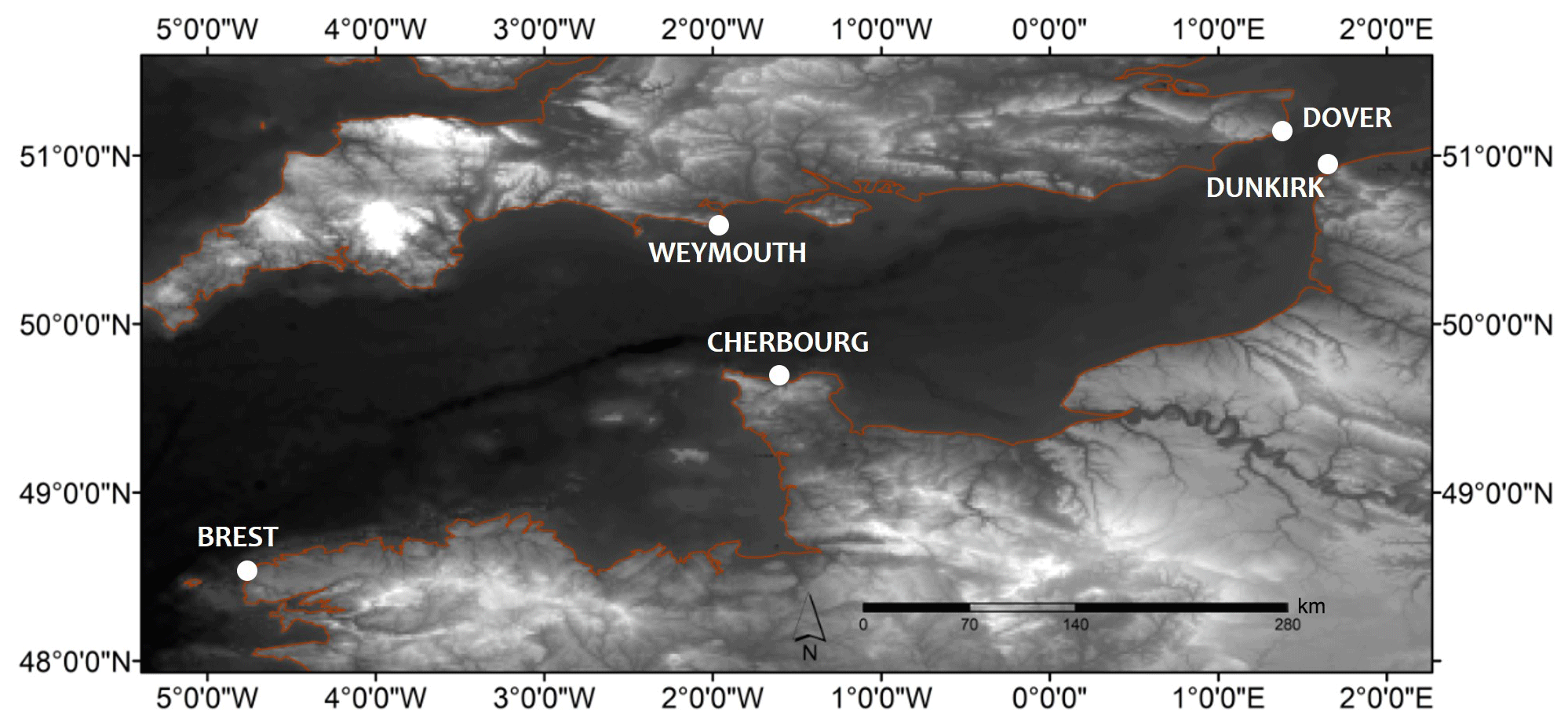
Figure 1 Geographical location of the study area and the different tide gauges along the English Channel coasts: Brest, Cherbourg and Dunkirk (NW France) and Dover and Weymouth (SW UK).

Two tide gauge sites along the UK coasts have been used: (1) Dover station, which is separated from Dunkirk by the North Sea, and (2) Weymouth station, symmetrical with respect to Cherbourg.

The French tide gauges are operated and maintained by the National French Centre of Oceanographic Data (SHOM) while the UK tide gauges are operated by the British Oceanographic Data Centre. All stations are referenced to the hydrographic zero level; they provide time series of hourly observation measurements until 2018.

Available data are summarized as the following: Brest (168 years between 1850 and 2018), Cherbourg and Dunkirk (54 years between 1964 and 2018), Dover (53 years between 1963 and 2018), Weymouth (28 years between 1990 and 2018).

The hourly measurements suffer from some gaps of daily length distributed along the time series. These gaps have been processed by the hybrid model for filling gaps developed by Turki et al. (2015b) by using the SLP as a covariate in the autoregressive moving average (ARMA) methods and the memory effects of the previous distribution of surges to estimate the missing values and fill the gaps. This model has been used in the recent works of Turki et al. (2019, 2020).

The large-scale atmospheric circulations are represented in this work by four different climate indices which are considered to be fundamental drivers in the Atlantic regions (Massei et al., 2017; Turki el al., 2019, 2020): the Atlantic Multidecadal Oscillation (AMO), the North Atlantic Oscillation (NAO), the zonal wind (ZW) component extracted at 850 hPa and the sea level pressure (SLP).

Monthly time series of climate indices have been provided by the NCEP-NCAR Reanalysis fields (http://www.esrl.noaa.gov/psd/data/gridded/data.ncep.reanalysis.derived.html, last access: 19 November 2020) until the year 2017. The different indices have been extracted during the same period of the sea level observations at the four stations Cherbourg, Dunkirk, Dover and Weymouth. For the longest time series of Brest (1850–2018), the use of climate indices has been limited according to their initial date availability (AMO: 1880–2017; NAO: 1865–2017; SLP: 1948–2017; ZW: 1865–2017).

3 Methodological approach

3.1 Extraction of residual sea level: “surges”

The total sea level height, resulting from the astronomical and the meteorological processes, exhibits a temporal nonstationarity which is explained by a combination of the effects of the long-term trends in the mean sea level, the modulation by the deterministic tidal component and the stochastic signal of surges, and the interactions between tides and surges. The occurrence of extreme sea levels is controlled by periods of high astronomically generated tides, in particular at interannual scales when two phenomena of precession cause systematic variation in high tides. The modulation of the tides contributes to the enhanced risk of coastal flooding. Therefore, the separation between tidal and non-tidal signals is an important task in any analysis of sea level time series. By the hypothesis of independence between the astronomical tides and the stochastic residual of surges, the non-linear relationship between the tidal modulation and surges is not considered in the present analysis. Using the classical harmonic analysis, the tidal component has been modelled as the sum of a finite set of sinusoids at specific frequencies to determine the determinist phase and amplitude of each sinusoid and predict the astronomical component of tides. In order to obtain a quantitative assessment of the non-tidal contribution in storminess changes, technical methods based on the MATLAB T_TIDE package have been applied to the sea level measurements, demodulated from long-term components (e.g. mean sea level, vertical local movement), for estimating year-by-year tidal constituents. A year-by-year tidal simulation (Shaw and Tsimplis, 2010) has been applied to the sea level time series to determine the amplitude and the phase of tidal modulations using harmonic analysis fitted to 18.61-, 9.305-, 8.85- and 4.425-year sinusoidal signals (Pugh, 1987). The radiational components have also been considered for the extraction of the stochastic component of surges (Williams et al., 2018).

3.2 Wavelet spectral analysis

The continuous wavelet transform (CWT) is generally used for data analysis in hydrology, geophysics and environmental sciences (Labat, 2005; Sang, 2013; Torrence and Compo, 1998). This technique produces the timescale with the means of the Fourier transform contour diagram in which the time is indicated on the x axis, the timescale (period) on the y axis and the variance (power) on the z axis.

Then, a wavelet multi-resolution analysis has been used to decompose the signal of monthly extreme surges into different internal components corresponding to different timescales. This decomposition consists of applying a series of iterative filtering to the signal by the use of low-pass and high-pass filters able to produce the spectral components describing the total signal. More details are presented in the recent works of Massei et al. (2017) and Turki et al. (2019).

In summary, the total signal has been separated into a relatively small number of wavelet components from high to low frequencies that altogether explain the variability of the signal; this will be illustrated later using the hourly measurements and the monthly maxima of surges.

The wavelet coherence has been calculated to investigate the relationship between the extreme surges and the climate oscillations by identifying the timescales where the two time series co-vary, even if they do not display high power. Here, a significance test has been implemented by the use of a Monte Carlo analysis based on an autocorrelation function of two time series (Grinsted et al., 2004).

3.3 Nonstationary extreme value model

Finally, and with the aim of addressing the nonstationary behaviour of extreme surges, the monthly maxima of the surges have been calculated and decomposed with the multi-resolution analysis. Then, a nonstationary extreme value analysis based on the GEV distribution with time-dependent parameters (Coles, 2001) has been implemented to model the series of the monthly maxima surges. There are several GEV families which depend on the shape parameter, e.g. Weibull (ε<0), Gumbel (ε=0) and Fréchet (ε>0). The three parameters of the GEV (i.e. location μ, scale ψ, shape ε) are estimated by the maximum likelihood function.

The nonstationary effect was considered by incorporating the selected climate indices (NAO, AMO, ZW and SLP) into the parametrization of the GEV models. The Akaike information criterion (AIC) has been used to select the most appropriate probability function models. The methods of maximum likelihood were used for the estimation of the distribution's parameters. The approach used considers the location (μ), the scale (ψ) and the shape (ε) parameters with relevant covariates, which are described by a selected climate index.

$$\begin{array}{}\text{(1)}& {\displaystyle }\mathit{\mu }\left(t\right)={\mathit{\beta }}_{\mathrm{0},\mathit{\mu }}+{\mathit{\beta }}_{\mathrm{1},\mathit{\mu }}{Y}_{\mathrm{1}}+\mathrm{\dots }+{\mathit{\beta }}_{n,\mathit{\mu }}{Y}_n\text{(2)}& {\displaystyle }\mathit{\psi }\left(t\right)={\mathit{\beta }}_{\mathrm{0},\mathit{\psi }}+{\mathit{\beta }}_{\mathrm{1},\mathit{\psi }}{Y}_{\mathrm{1}}+\mathrm{\dots }+{\mathit{\beta }}_{n,\mathit{\psi }}{Y}_n\text{(3)}& {\displaystyle }\mathit{\epsilon }\left(t\right)={\mathit{\beta }}_{\mathrm{0},\mathit{\epsilon }}+{\mathit{\beta }}_{\mathrm{1},\mathit{\epsilon }}{Y}_{\mathrm{1}}+\mathrm{\dots }+{\mathit{\beta }}_{n,\mathit{\epsilon }}{Y}_n\end{array}$$

Here β0, β1, …, βn are the coefficients, and Yi is the covariate represented by the climate index. For each spectral component, only one climate index can be used to be introduced into the parameters μ, ψ and ε of the nonstationary GEV model (into one of them, into two of them or into the three parameters). With the aim of optimizing the best use of the most appropriate climate index (detailed in Sect. 3.4) into the different GEV parameters, a series of sensitivity analyses were implemented for each timescale. The AIC measures the goodness of fit of the model (Akaike, 1973) with the relation AIC $=-\mathrm{2}l+\mathrm{2}K$, where l is the log-likelihood value estimated for the fitted model and K is the number of the model parameters. Higher-ranked models should result from lower AIC scores.

3.4 Determination of the most appropriate climate oscillation connected to each extreme-surge timescale for GEV models

As suggested previously, the main hypothesis presented in this research is that effects of the physical mechanisms on the extreme surges vary according to the timescale, and each scale should be related to a given climate oscillation.

This hypothesis has been investigated using two approaches.

1. The spectral approach was based on the use of wavelet techniques (wavelet multi-resolution and wavelet coherence as detailed in Sect. 3.2) for optimizing the physical relationship between the climate index and the extreme surges at each timescale.

   The bootstrap is a resampling technique used to estimate the sampling distribution of an estimator of sample statistics by drawing randomly with replacement from a set of data points.

   Here, a bootstrap approach has been applied to assess the statistical significance of the correlation between the spectral component of the extreme surges and the climate oscillation at each timescale. By resampling the time series 10 000 times, the extreme surges have been simulated and compared to the original records; the 95 % confidence intervals have been considered to extract the best climate information fitting the extreme surges (Villarini et al., 2009).

2. A Bayesian estimation has been used to make inferences from the likelihood function. The reason behind the choice of this approach is overcoming the limitation of short time series with small size, like in the case of Weymouth station where the measurements cover the period from 1991 to 2018. A Markov chain Monte Carlo (MCMC) technique, implemented in the evbayes package within R software, has been used basing on multiple simulations (the number of simulations varies as a function of the length of the time series).

For each spectral component, a sample of 100 000 simulations has been modelled by GEV using a given climate index. The upper and lower quantiles of the posterior probability distribution for the parameters of the MCMC sample are taken. The goodness of fit has been taken as a function of the values of the upper and the lower quantiles; the best results have been considered when these values are higher than 92.5 % and lower than 5.2 %, respectively.

Both approaches have been used to select the most appropriate atmospheric physical mechanism for each timescale of extreme surges. Then at each timescale (i.e. spectral component), the selected mechanism (i.e. the climate oscillation in this case) has been used as a covariate for modelling the extreme surge by the implemented nonstationary GEV models. The best use of the covariate in the different GEV parameters (location, scale and shape) has been investigated by means of AIC.

Once the best GEV models were defined for each timescale, a series of simulations were carried out to compare modelled and observed surges.

This Bayesian inference has been also used to calculate (1) the return levels of the nonstationary simulated surges which were compared to those of the observed ones and (2) the confidence interval (CI) assessing the goodness of this comparison.

4 Multi-timescale variability of extreme surges

The variability of the monthly extreme surges along the English Channel coasts has been investigated using the continuous wavelet transform (CWT). In the spectrum of Fig. 2, the colour scale represents an increasing power (variance) from red to blue and pink. The CWT diagrams highlight the existence of several scales for all sites with different ranges of frequencies: the interannual scales of ∼1.5, ∼2–4 and ∼5–8 years and the interdecadal scale of ∼12–16 years.

The variability of surges is clearly dominated by the interannual frequencies (∼1.5, ∼2–4, ∼5–8 years), explaining a mean variance between 32 % and 25 % of the total energy (Table 1). In Dover and Weymouth, the low frequencies of ∼2–4 years are well-structured with a mean explained variance of 9.5 % while it is of 7 % for ∼5–8 years. These percentages decrease slightly for the French sites to 8 % and 5 %, respectively. At ∼1.5 years, the explained variance is higher than 16 % and 13 %, respectively, for the UK and French coasts. The interdecadal frequency of ∼12–16 years varies between 2 % and 4 % from the total signal. This frequency is not observed in the shortest time series of Weymouth (Table 1).

The interannual variability (timescales higher than ∼1 year) seems to be highly represented in the monthly extrema CWT (Fig. 2). This is not the case for the monthly mean surges (Fig. 3a) where most of the power spectrum is concentrated on the annual cycle with an explained variance higher than 50 %.

The time-dependent PDF of the monthly mean and maximum surges over a period of 10 years, for illustration purpose, is displayed in Fig. 3b. The ∼1-year component of monthly mean surges is largely manifested with a pronounced variation in the Gaussian curves in time; such variations take wavelengths of approximately ∼2 and ∼4 years. This result exhibits that the interannual frequencies of ∼2 and ∼4 years are modulated within the annual mode for the mean surges while they are implicitly quantified for the monthly maxima.

Figure 2 CWT of monthly maxima of surges in Brest, Cherbourg, Dunkirk, Dover and Weymouth.

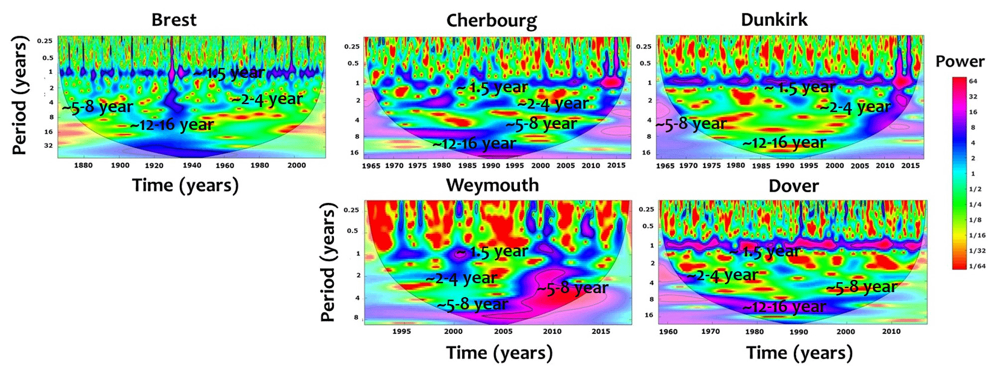
Figure 3 Multiscale variability of the monthly mean and maximum surges in Brest. (a) CWT of monthly mean surges. (b) Interannual variability of monthly and extreme surges.

Results have been explored to investigate the nonstationary dynamics of surges at different timescales. We have applied the wavelet multi-resolution decomposition of monthly extrema for each site. The process has resulted in the separation of several components with different timescales. In this research, we are interested in the timescales higher than 1 year, i.e. traduced by three interannual scales (∼1.5, ∼2–4 and ∼5–8 years) and an interdecadal scale of ∼12–16 years. We focused only on the interannual and the interdecadal scales whose fluctuations correspond to the oscillation periods less than half the length of the record and exhibit a high-energy contribution to the variance of the total signal. The lowest frequency, corresponding to ∼12–16 years, is easily calculated from the longest record of Brest.

Figure 4 shows a series of oscillatory components of surges from interannual to interdecadal scales, not easily quantified by a simple visual inspection of the signal. High similarities between the different sites have been highly observed for the interannual and the interdecadal scales of ∼5–8 and ∼12–16 years while they are less pronounced at the small scales of ∼1.5 years. At this timescale, the differences in the extreme surges can be explained by local physical phenomena controlling their dynamics. Such processes are mainly induced by combining the effects of meteorological and oceanographic forces including changes in atmospheric pressures and wind velocities in shallow-water areas. Beyond ∼1.5 years, the variability of extreme surges at larger scales seems to be quite similar in terms of frequency and amplitude for the five sites.

Such large variability reveals the physical effects of a global contribution related to climate oscillations. The extent of the large-scale oscillations is not strictly similar and changes according to the timescale variability since the dynamics of surges is not necessarily related to the same type of atmospheric circulation process. This relationship will be addressed later in the second part of this section.

Here, the multiscale variability of extremes has been investigated from the spectral components of surges along the English Channel coasts. This signal has been linearly extracted from the total sea level, provided by tide gauges, by the use of the classical harmonic analysis and thanks to the assumption that the water level is the sum of the mean sea level, tides and surges. This assumption approximates the quantification of both components in the English Channel where the significant tide–surge interactions (Tomassin and Pirazzoli, 2008) and the effects of the sea level rise on tides and surges are important (e.g. Idier et al., 2017). Neglecting this non-linear interaction between the surges, tides and sea level rise suggests some uncertainties in the estimation of the high frequencies of the spectral components between daily and monthly scales, which is not the focus of the present work where the interannual and the interdecadal scales are investigated.

Similar interannual timescales have been observed along the French coasts of Dunkirk, Le Havre and Cherbourg in Turki et al. (2020) where the intermonthly and interannual variability of 48-year hourly surges has been investigated. They have demonstrated that the timescales smaller than ∼1.5 years are differently manifested between the different sites. These differences have been associated with the local variability of surges induced by combining the effects of meteorological and oceanographic forces including changes in atmospheric pressures and wind velocities in shallow-water areas. As demonstrated in Turki et al. (2020), the mean explained variance of the interannual fluctuations (∼1.5, ∼2–4 and ∼5–8 years) is around 25 % of the total surges along the French coasts (Table 1). This value is higher than 32 % in Weymouth and Dover while the explained variance of the interdecadal scales (∼12–16 years) is also more important with 3.5 % (compared to 2 % for the French coasts).

Table 1 The explained variance expressed as a percentage of total variance of monthly extreme surges. The lowest frequency of ∼12–16 years is not observed in Weymouth.

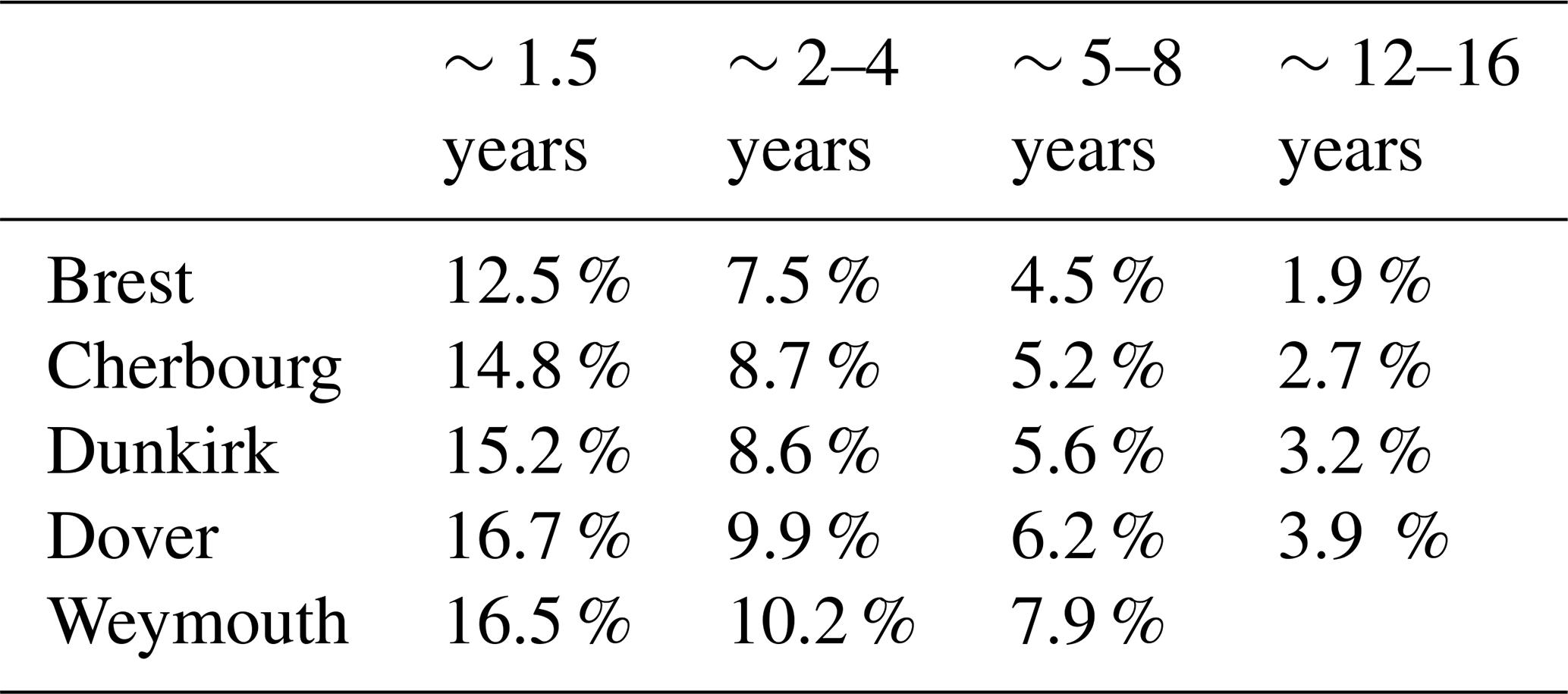
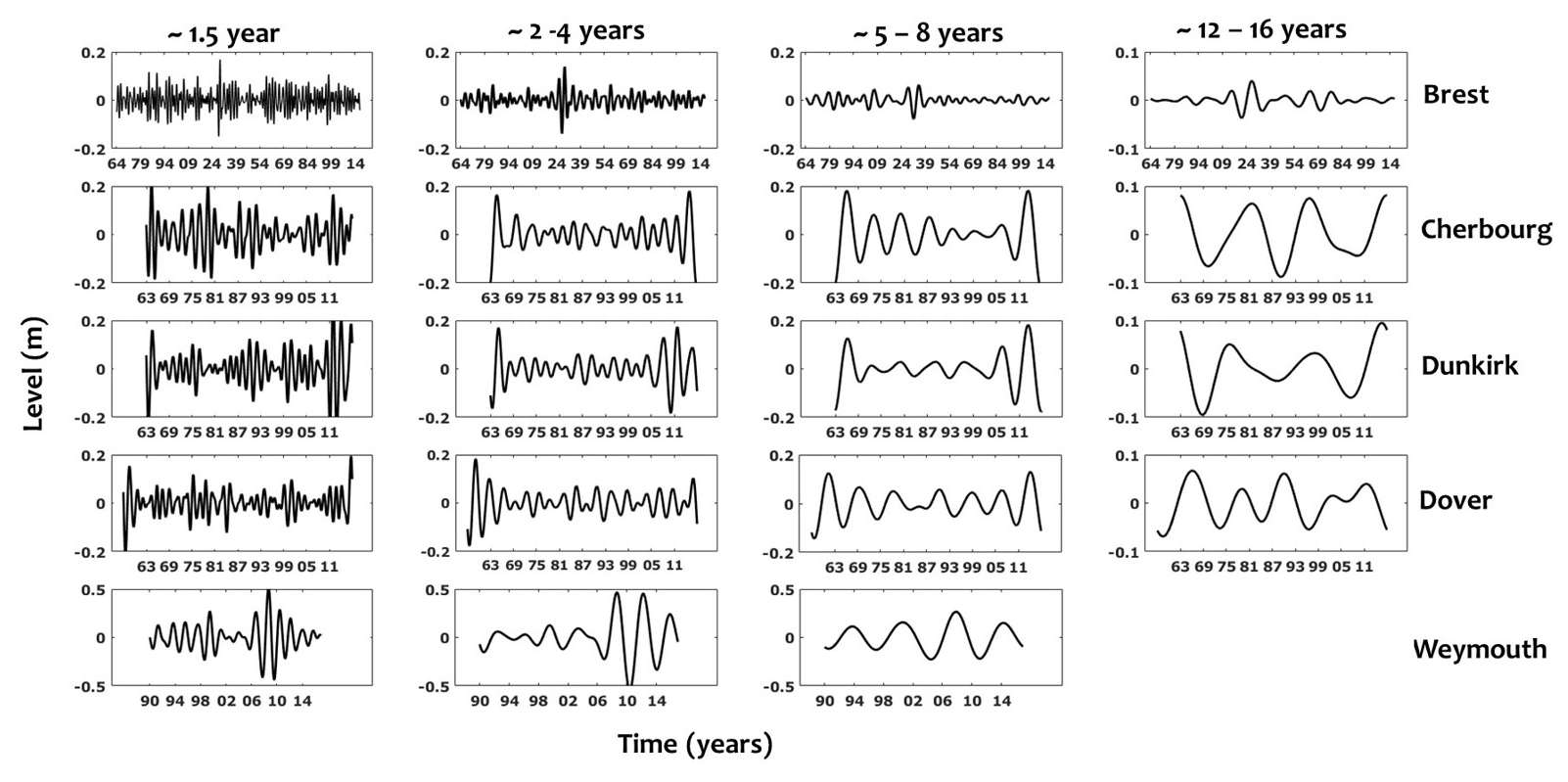
Figure 4 Wavelet details (components) resulting from the multi-resolution analysis of surges at the interannual (∼1.5, ∼2–4 and ∼5–8 years) and interdecadal (∼12–16 years) timescales for all sites (Brest, Cherbourg, Dunkirk, Dover and Weymouth).

The interdecadal variability (∼ 12–16 years) of extreme surges has been evidenced by Turki et al. (2019) in the Seine Bay (NW France). Strong physical relations have been exhibited between the interdecadal time of ∼ 12–16 years and the exceptional stormy events produced with surges higher than the 10-year-return-period level. The connections between the low-frequency components and the historical record of the exceptional events suggested that storms would occur differently according to a series of physical processes oscillating at multi-timescales; these processes control their frequency and their intensity (Turki el al., 2019).

Accordingly, the multiscale variability of extreme surges exhibits a nonstationary behaviour modulated by a non-linear interaction between the different interannual and interdecadal timescales. Then, assessing the effect of the nonstationary behaviour at different timescales is important for improving the estimation of extreme values and the projection of storm surges.

5 Large-scale North Atlantic climate oscillations and their link to extreme surges in the English Channel

In this part, a new hybrid approach combining the spectral analysis and the nonstationary GEV models has been used to investigate the connection between the multi-timescale variability of local surges and the large-scale North Atlantic climate oscillations.

As proposed by Turki et al. (2019, 2020), the hypothesis used in the present work is that the multi-timescale variability of the local extreme surges should be strongly related to different climate teleconnections induced by a complex contribution of many physical mechanisms. This non-linear relationship varies according to each timescale, which depends on a specific large-scale oscillation of atmospheric circulation.

5.1 To what extent would large-scale climate oscillations link extreme surges?

The wavelet coherence (WC) diagrams between the monthly maxima of surges and the different climate indices of SLP, ZW, NAO and AMO, introduced previously as the main atmospheric circulation within the English Channel, are illustrated, respectively, in Figs. 5, 6, 7 and 8. Results provided by these diagrams highlight the following.

1. The connection between the climate oscillations and the extreme surges is manifested differently as a function of the timescale. From a visual inspection of the different spectra illustrated by the WC, the most significant correlations of extreme surges have been identified with SLP, ZW, NAO and AMO, respectively, at ∼ 1.5, ∼ 2–4, ∼ 5–8 and ∼ 12–16 years.

2. Each timescale mainly exhibits strong links with its associated climate index (explained variance between 55 % and 80 %) and weak ones with other indices (explained variance between 15 % and 5 %). Table 2 summarizes the contribution of the different climate oscillations in the different interannual and interdecadal timescales of extreme surges. Here, mean values between the different sites are presented.

For example, SLP diagrams reveal significant relationships with ∼ 1.5-year surges (well-structured forms with high concentration of pink and blue colours in Fig. 5); limited correlations, locally positioned in time, have been observed at ∼ 2–4- and ∼ 5–8-year scales. ZW shows strong correlations with interannual surges at ∼ 2–4 years (blue to pink colour at this scale; Fig. 6) and other correlations at smaller and larger timescales of ∼ 1.5 and ∼ 5–8 years, respectively. Similarly, NAO presents high links with ∼ 5–8-year surges and small relations with ∼ 2–4 and ∼ 1.5 years (Fig. 7).

The ∼ 1.5-year scale highlights strong correlations with SLP with an explained variance of 75 %; 25 % of this scale should be explained by the influence of other climate oscillations (basically ZW and NAO with a mean explained variance of 10 % and 6 %, respectively; Table 2) and the combining effects of locally driven forcing induced by winds and waves.

A total of 65 % of the ∼ 2–4-year scale is correlated with ZW while 5 % and 12 % is explained by the effect of NAO and SLP, respectively. The effects of NAO on the ∼ 5–8 years vary between 55 % and 65 %; minor influence at this scale has been observed, with SLP and ZW explaining a mean variance of 13 %. The interannual scales of surges are slightly influenced by AMO oscillations with low values of variance lower than 1 % (Table 2).

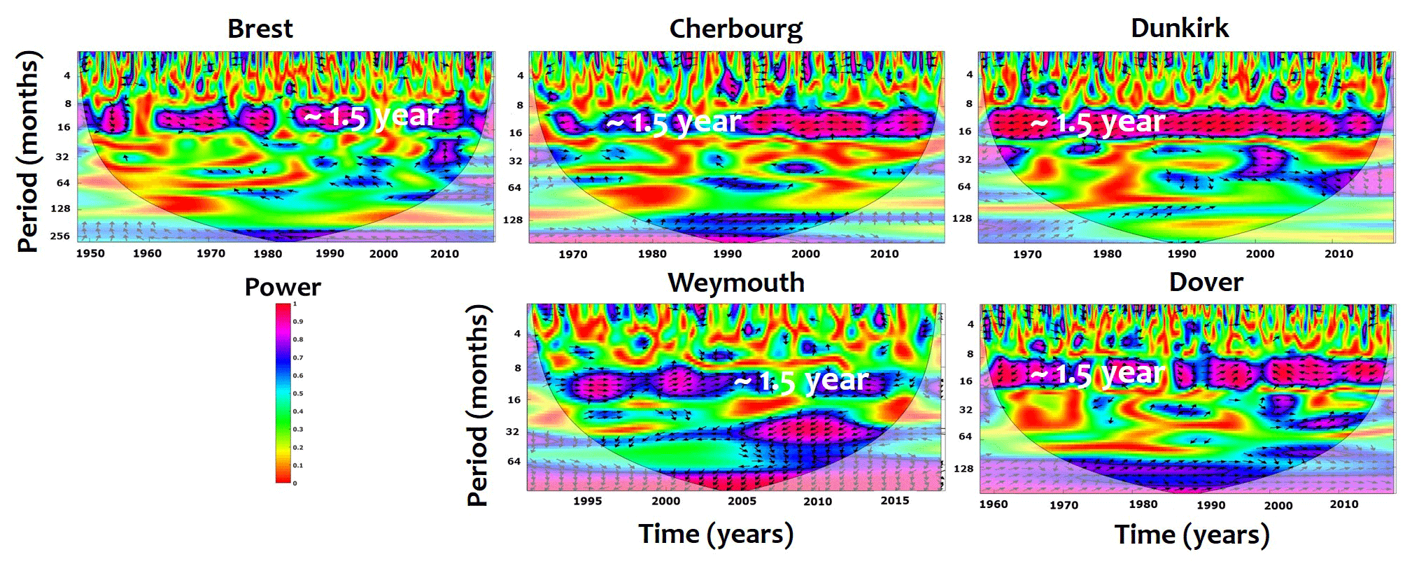
Figure 5 Cross-wavelet correlations between monthly extrema of surges and sea level pressure (SLP).

Figure 6 Cross-wavelet correlations between monthly extrema of surges and zonal wind (ZW).

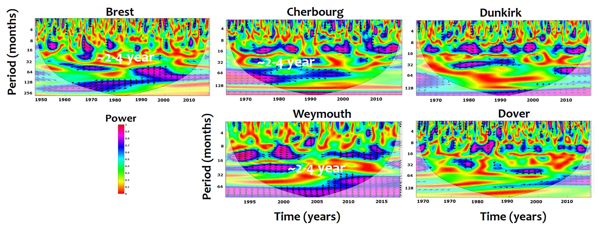
Figure 7 Cross-wavelet correlations between monthly extrema of surges and the North Atlantic Oscillation (NAO).

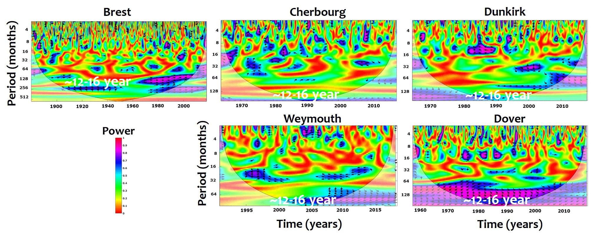
Figure 8 Cross-wavelet correlations between monthly extrema of surges and the Atlantic Multidecadal Oscillation (AMO).

Table 2 The mean explained variance expressed as a percentage of total variance provided by the wavelet coherence between the extreme surges and the climate oscillations (SLP, ZW, NAO, AMO).

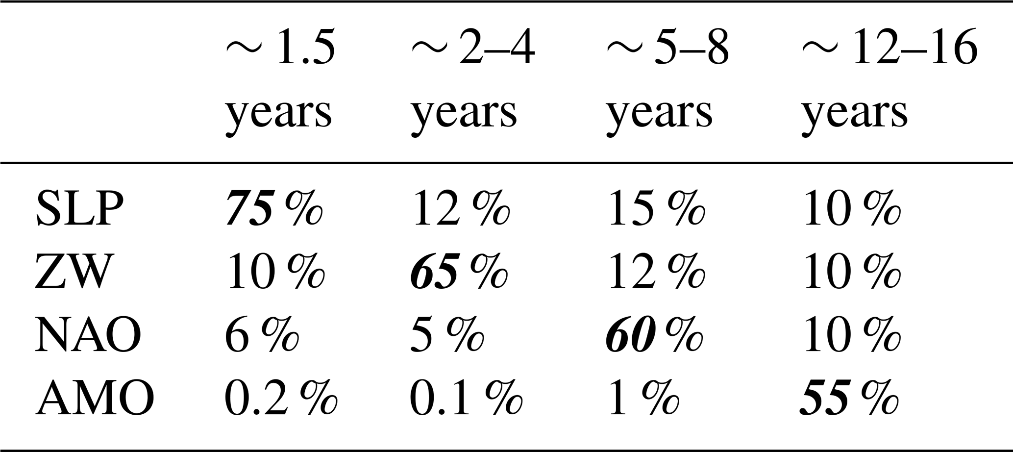
At interdecadal scales of ∼ 12–16 years, the extreme surges are mainly controlled by the AMO oscillations with a mean explained variance of 80 % while the effects of NAO are limited to 10 % (Fig. 8).

Figure 9 displays the spectral components of the four climate oscillations, provided by a multi-resolution analysis, together with the spectral components extracted from the extreme surges (Fig. 4) with the aim to quantify the different connections between both variables at the interannual and the interdecadal timescales.

For each timescale, a bootstrap approach has been applied to assess the statistical significance of the correlation between the spectral component of the extreme surges and the climate oscillation. By resampling the time series 10 000 times, 95 % confidence intervals (CIs) have been considered to extract the best climate information fitting the extreme surges (Villarini et al., 2009).

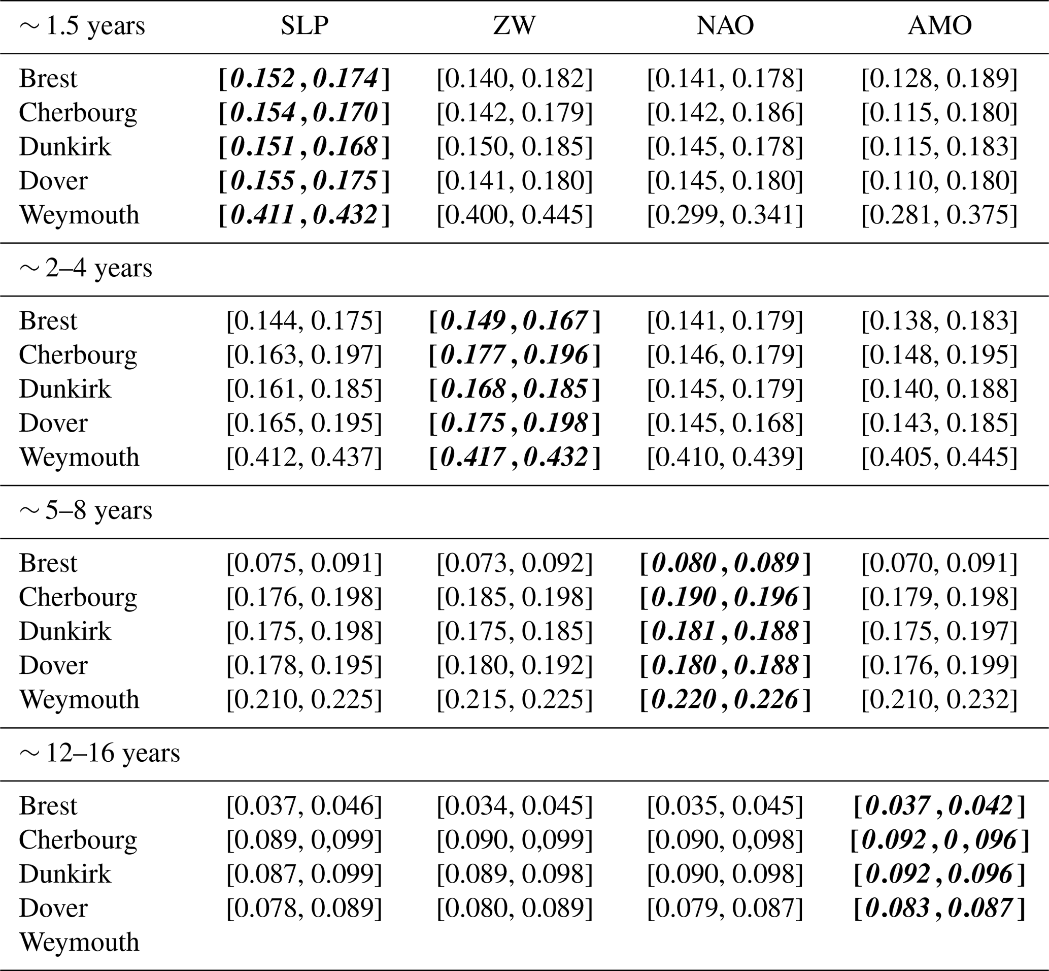
Results of the 95 % CI, applied to the maximum values and provided by the bootstrap technique, for the different possible connections between a given scale of extreme surges and a climate oscillation, extracted at the timescale of extreme surges, are illustrated in Table 3. For each connection, the lower and the upper bounds of the 95 % CI, calculated for the maximum values, are calculated (values in the square brackets in Table 3). The width of the CI between both bounds reveals the statistical significance of the simulations and the goodness of the correlations. According to these results, the width of the CI is important for the small timescales (high frequencies of ∼ 1.5 and ∼ 2–4 years) with a mean of 0.05 and a maximum of 0.09. It decreases for the large timescales (low frequencies of ∼ 5–8 and ∼ 12–16 years) to 0.012 and 0.022 of mean and maximum values, respectively.

The smallest widths are observed for the connection between ∼ 1.5-year extreme surges and SLP, ∼ 2–4-year extreme surges and ZW, ∼ 5–8-year extreme surges and NAO and ∼ 12–16-year extreme surges and AMO (italics in Table 3). For the large timescales (low frequencies), small widths (lower than the mean value 0.012) are also observed with other climate oscillations, different from the most appropriate one showing the most significant correlation with extreme surges. For these scales, the variability of extreme surges is mainly controlled by a given physical mechanism, related to a climate oscillation, and partly affected by the contribution of other oscillations which could interact with the different large driven forces. Such interaction between the different climate oscillations has also been shown in Table 2.

The best correlation of each extreme-surge component (i.e. ∼ 1.5, ∼ 2–4, ∼ 5–8 and ∼ 12–16 years) with the most appropriate climate oscillation (i.e. SLP, ZW, NAO and AMO) is illustrated in Fig. 9. The interannual variability and the interdecadal variability of extreme surges and their multiscale connection with the climate oscillations highlight the non-linear relationship between large and local scales.

Table 3 Analysis of the statistical significance of the correlation between the spectral component of the extreme surges and the climate oscillation at each timescale for the different stations is shown. The 95 % confidence intervals (applied for the maximum values) from the bootstrap technique are shown in square brackets. The most significant correlations, shown by the most limited (smaller) 95 % CI between the lower and the upper bounds, are illustrated in italics. The lowest frequency of ∼ 12–16 years is not observed in Weymouth.

Therefore, the interannual and the interdecadal extreme surges have proven to be strongly related to different composites of oscillating atmospheric patterns. Such composites seem to be not necessarily similar for the different timescales. The use of a multi-resolution approach to investigate the dynamics of the extreme surges in the downscaling studies proves to be useful for assessing the nonstationary dynamics of the local extreme surges and their non-linear interactions with the large-scale physical mechanisms related to climate oscillations.

Investigating the complex relationships between the climate oscillations and the multi-timescale surges has exhibited a multimodel climate ensemble that should be used to better understand this complexity.

The interannual connections between the local hydrodynamics and the climate variability have been investigated in numerous previous works focused on the atmospheric circulation with different related mechanisms (e.g. Feliks et al., 2011; López-Parages and Rodríguez-Fonseca, 2012; Zampieri et al., 2017). As demonstrated by the recent works of Turki et al. (2019, 2020), the effects of SLP oscillations on the ∼ 1.5-year variability of extreme surges are described by dipolar patterns of high–low pressures with a series of anomalies which are probably induced by some physical mechanisms linked to the North Atlantic and ocean–atmosphere circulation oscillating at the same timescale.

The SLP fields combined with the baroclinic instability of wind stress have been related to the Gulf Stream path as given by NCEP reanalysis (Frankignoul et al., 2011); the dominant signal is a northward (southward) displacement of the Gulf Stream when the NAO reaches positive (negative) extrema. Daily mean SLP fields have been used by Zampieri et al. (2017) to analyse the influence of the Atlantic sea temperature variability on the day-by-day sequence of large-scale atmospheric circulation patterns over the Euro-Atlantic region. They have associated the significant changes in certain weather regime frequencies with the phase shifts of the AMO. For hydrological applications, several works have investigated the multiscale relationships between the local hydrological changes and the climate variability. Lavers et al. (2010) associated the 7.2-year timescales the SLP patterns which are not exactly reminiscent of the NAO and define centres of action which are shifted to the north.

Regarding the ZW (u850), results have shown its correlation with the interannual scales of ∼ 2–4-year extreme surges as also suggested in the recent findings of Turki et al. (2020). Its influence has also been proven at smaller (∼ 1.5 years) and larger scales (5–8 years). Additionally, for extreme surges, the interaction between the ZW and the temperature at different timescales has been highlighted in some previous research (e.g. Andrade et al., 2012; Seager et al., 2003; Woodworth et al., 2007). Along UK and northern English Channel coasts, changes in trends of extreme waters and storm surges have been explained by variations in energy pressure and ZW variability in addition to thermosteric fluctuations linked to NAO (Woodworth et al., 2007).

Andrade et al. (2012) have used the component of ZW at 850 hPa to investigate the positive and the negative phases of the extreme temperatures in Europe and their occurrence in relation with the large-scale atmospheric circulation. They suggested that both phases are commonly connected to strong large-scale changes in zonal and meridional transports of heat and moisture, resulting in changes in the temperature patterns over western and central Europe (Corte-Real et al., 1995; Trigo et al., 2002). The physical connections between ZW and the extreme events from 11 global climate model runs have been demonstrated by the studies from Mizuta (2012) and Zappa et al. (2013); they have suggested the complex relationship between the climate oscillation and the jet stream activity. They have found a slight increase in the frequency and strength of the storms over central Europe and decreases in the number of the storms over the Norwegian and Mediterranean seas.

Figure 9 Wavelet details of monthly extreme surges (black lines), at the interannual (∼ 1.5, ∼ 2–4 and ∼ 5–8 years) and interdecadal (∼ 12–16 years) timescales for all sites (Brest, Cherbourg, Dunkirk, Dover and Weymouth), correlated to the spectral component of climate oscillations associated with the different indices SLP, ZW, NAO and AMO (grey line). Only the connection maximizing the correlation coefficient between a selected climate index and the component of surges (from interannual to interdecadal timescales) is presented (the normalized values have been calculated to superpose both signals).

The NAO is considered to be an influencing climate driver for the large-scale atmospheric circulation, as suggested by other research (e.g. Marcos et al., 2009; Philips et al., 2013).

The existence of long-term oscillations originating from large-scale climate variability and thus controlling the interannual extreme surges has been highlighted from investigating the low frequencies of the sea levels along the English Channel. This is in agreement with the results recently demonstrated by Turki et al. (2020) and the present finding exhibiting the strong links between NAO oscillations and the ∼ 5–8-year extreme surges along the English Channel coasts.

The physical mechanisms related to the effects of the continuous changes in NAO patterns on the sea level variability have been addressed in several studies (e.g. Marcos et al., 2009; Tsimplis et al., 2009). At the interannual scales, the key role of the NAO in the sea level variability has been explained by some previous works: Philips et al. (2013) investigated the influence of the NAO on the mean and the maximum extreme sea levels in the Bristol Channel and Severn Estuary. They have demonstrated that wind speeds rise when the negative NAO increases, resulting in low wind speeds. Then, the correlation between the low–high extreme surges and the NAO in the Atlantic has demonstrated a proportionality between NAO values and the augmentation in the winter storms. Feliks et al. (2011) defined significant oscillatory timescales of ∼ 2.8, ∼ 4.2 and ∼ 5.8 years from both observed NAO index and NAO atmospheric marine boundary layer simulations forced with sea surface temperature (SST); they have suggested that the atmospheric oscillatory modes should be induced by the Gulf Stream oceanic front.

Strong correlations between the monthly extreme surges and the AMO oscillations have been identified at the timescale of 12–16 years (Figs. 8 and 9; in particular for Brest). Since the period of the 1990s, the AMO and the extreme surges oscillate in opposition of phase. This shift should be explained by a substantial change in European climate manifested by cold wet and hot dry summers in northern and southern Europe, respectively; as discussed by Sutton and Dong (2012). They have demonstrated that the patterns, identified from European climate change around the 1990s, are synchronized with changes related to the North Atlantic Ocean.

Other weak links with the AMO have been identified at the interannual timescales of ∼ 5–8 years along the studied sites. In agreement of previous works (e.g. Enfield et al., 2001; Zampieri et al., 2013, 2017), the effects of the AMO oscillations are mainly manifested at the interannual timescale to control the variability of hydrological (e.g. rainfall) and oceanographic (e.g. surges) variables. Generally, the climate oscillations of AMO are associated with the SST variability with a time cyclicity of about 65–70 years (e.g. Delworth and Mann, 2002; Enfield et al., 2001). During the warming periods of the 1990s, the AMO shifts from the negative to the positive phases in the Northern Hemisphere, corresponding to cold and warm periods (e.g. Gastineau et al., 2012; Zhang et al., 2013). This shift can be responsible for changes in the hydrodynamic conditions (e.g. Zampieri et al., 2013).

The influence of the AMO oceanic low frequencies in the modulation of the mechanisms of the atmospheric teleconnections at the interannual timescale has been investigated in many previous works (e.g Enfield et al., 2001). At decadal timescales, the existing relationships between the winter NAO and the AMO variability is more complex (e.g. Peings and Magnusdottir, 2014).

The effects of the AMO-driven climate variability on the seasonal weather patterns have been investigated by Zampieri et al. (2017) in Europe and the Mediterranean. They have demonstrated significant changes in the frequencies of weather regimes influenced by the AMO shifts which are in phase with seasonal surface pressure and temperature anomalies. Such regimes, produced in spring and summer periods, are differently manifested in Europe with anomalous cold conditions over western Europe (Cassou et al., 2005; Zampieri et al., 2017).

In summary, four atmospheric oscillations have proven to be significantly linked to the interannual and interdecadal variability of extreme surges. This physical link varies according to the timescale, exhibiting a non-linear interaction of the same oscillations with other scales. Such non-linear behaviour depends on the dynamics of the different sequences of the atmospheric and water vapour transport patterns during the month prior to the sea level observations (e.g. Lavers et al., 2015). As suggested by Turki et al. (2020), the atmospheric circulation acts as a regulator controlling the multiscale variability of extreme surges with a non-linear connection between the large-scale atmospheric circulation and the local-scale hydrodynamics. This multi-timescale dependence between the local extreme dynamics and the internal modes of climate oscillations is still under debate. Understanding these physical links, even their complexities, is useful to improve the estimation of the extreme values in coastal environments, which is the objective of the next part.

5.2 Nonstationary modelling of extreme surges

In this part, stationary and nonstationary extreme value analyses based on GEV distribution with time-dependent parameters (Coles, 2001) have been implemented to separately model the different spectral components of extreme surges. Four GEV stationary (GEV0) and nonstationary (GEV1, GEV2 and GEV3) models have been applied to each timescale and each site. The GEV distribution uses the maximum likelihood method by parametrizing the location, scale and shape of the model. We have used the “trust region reflective algorithm” for maximizing the log-likelihood function (Coleman and Li, 1996).

The connections between the climate oscillations and the monthly maxima at the different timescales (Fig. 9), preliminary presented in Sect. 5.1, have been explored for the implementation of the nonstationary GEV models. Indeed, multiple simulations of Markov chain Monte Carlo (MCMC) techniques based on Bayesian approaches have been employed for extreme-surge components (i.e. ∼ 1.5, ∼ 2–4, ∼ 5–8 and ∼ 12–16 years provided by the multi-resolution wavelet decomposition) to identify the best covariates of climate oscillation for parametrizing the nonstationary GEV models. Most of the simulations have mainly supported the results outlined in the previous section: the ∼ 1.5 years of SLP, ∼ 2–4 years of ZW, ∼ 5–8 years of NAO and ∼ 12–16 years of AMO oscillations are considered the best covariates for modelling, respectively, the ∼ 1.5, ∼ 2–4, ∼ 5–8 and ∼ 12–16 years of monthly extreme surges.

Once the climate covariate has been selected for each timescale, three nonstationary models have been used by introducing the climate information as a covariate into (1) the location parameter (GEV1); (2) both location and scale parameters (GEV2); and (3) all location, scale and shape parameters (GEV3). The structure of the most appropriate nonstationary GEV distribution has been selected by choosing the most adequate parametrization that minimizes the Akaike information criterion (Akaike, 1974). The goodness of fit for each model has been checked through the visual inspection of the quantile–quantile (Q–Q) plots (Fig. 10); these plots compare the empirical quantiles against the quantiles of the fitted model. Any substantial departure from the diagonal indicates inadequacy of the GEV model.

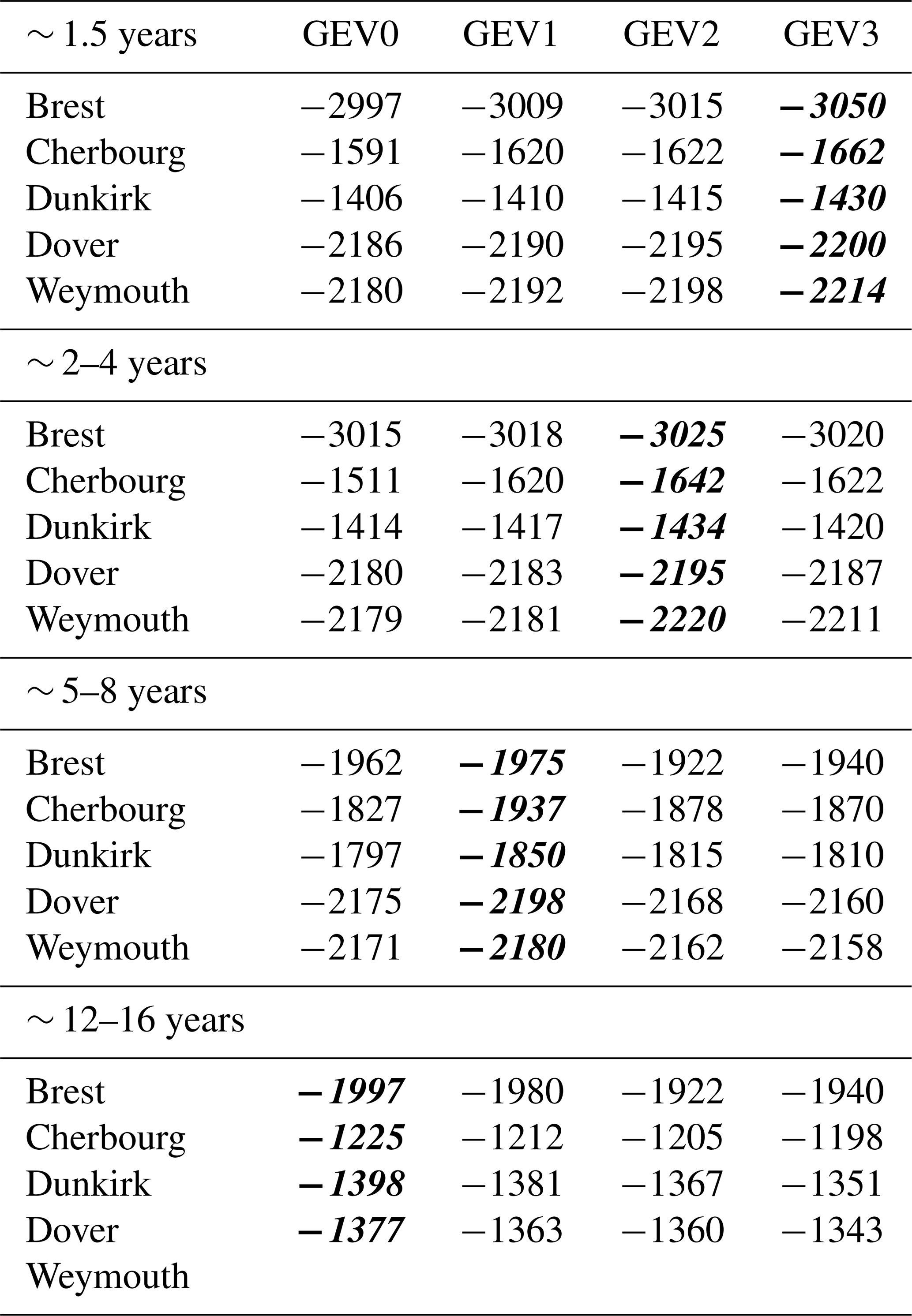
At the interannual scales and for all sites, results provided by the nonstationary GEV1–3 reveal a better performance (the lowest values of AIC) of extreme estimation compared to the stationary models of GEV0 and give the most appropriate distributions by the use of the large-scale climate covariates for specific oscillating components of extreme surges. Nevertheless, this improvement from the stationary to the nonstationary models has not been clearly observed for the interdecadal scales where the extreme estimation, provided by the different GEV models, is very similar (Table 3). The lowest values of AIC have been shown by GEV3 for ∼ 1.5 years, GEV2 for ∼ 2–4 years and GEV1 for ∼ 5–8 years (Table 4). The Q–Q plots for all timescales of the monthly maxima in Brest are illustrated in Fig. 10; they confirm the suitability of the selected models.

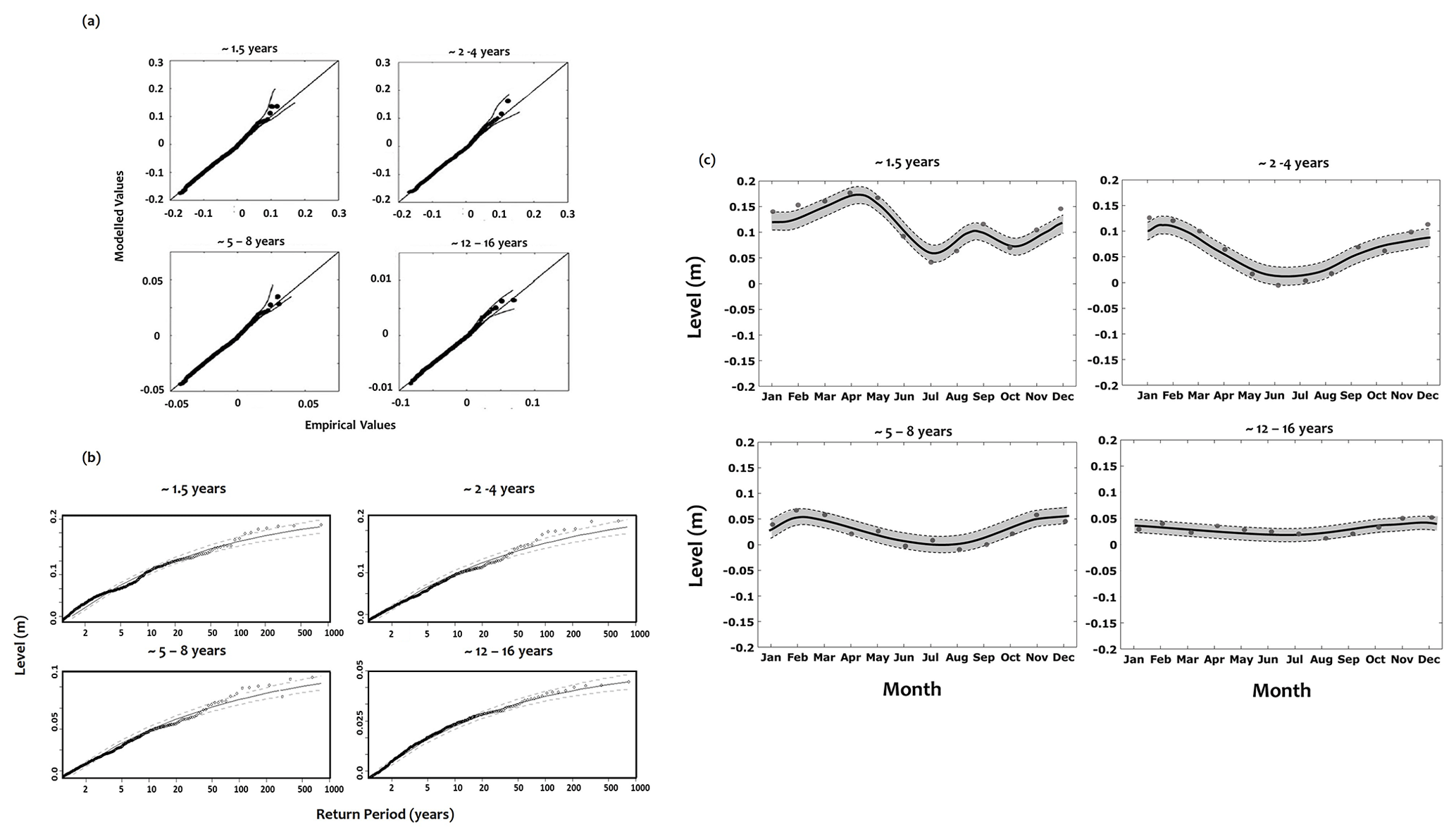
Figure 10 (a) The quantile plot between observed and modelled extreme surges by the use of the best GEV models, at different timescales, for the case of Brest. (b) The return level of extreme surges estimated for Brest using the best GEV models. The 95 % confidence interval is presented with the dashed black line. (c) The 50-year return level of monthly values using the original data (grey circles) and the best nonstationary GEV model at Brest (solid black line). The lower and the upper limits of the 95 % confidence interval calculated using the Bayesian method (dashed black line). The associated confidence area is represented by the grey shaded area.

Accordingly, the nonstationary GEV models have exhibited high improvements at the interannual scale where the AIC scores have significantly decreased by introducing the climate information into the parametrization of the model. Such consideration varies as a function of the spectral components; it concerns all parameters for the smallest scale of ∼ 1.5 years, both location and scale parameters for ∼ 2–4 years and only the location parameter for the largest scale of ∼ 5–8 years.

Then, the large-scale oscillations introduced for the implementation of GEV parameters depend on the timescale for all sites, exhibiting a high nonstationary behaviour of the small interannual scale (∼ 1.5 years), which decreases at the large interannual scale (∼ 5–8 years) and becomes non-significant at the interdecadal scale (∼ 12–16 years).

The use of the time-varying GEV parameters at the interannual scales (∼ 1.5 and ∼ 2–4 years) exhibits the relationship between the mode and the standard deviation of the GEV distributions associated with the location and the scale parameters, respectively.

The different implications of both parameters for estimating the interannual extreme surges reveal cyclic variations and timescale modulations related to the large-scale climate oscillations. As documented in previous works (e.g. Menendez and Woodworth, 2010; Masina and Lamberti, 2013), the location and the scale parameters used for improving the nonstationary estimation of the extreme water levels highlight a series of annual and semi-annual evolutions. They have reported that the seasonal cycles of the location parameter are related to tow maxima of water levels, in early March and September produced during equinoctial spring tides, while the seasonal cycles of the scale parameter are associated with an increase in storms during wintry episodes. Here, we focus on the stochastic signal of surges at scales larger than 1 year. The SLP and the ZW frequencies, introduced in the location and the scale parameters of nonstationary GEV models, determine an enhancement in the prediction of the interannual scales. The shape parameter, implied for the estimation of the ∼ 1.5-year extreme surges, derives from its determination of the upper tail distribution behaviour. The time-varying shape parameter uses the ∼ 1.5-year SLP exhibiting alternating negative and positive oscillations.

Despite its critical significance, the shape GEV parameter has revealed its relationships with basin attributes in hydrological applications and regional flood frequency analysis (e.g. Tyralis et al., 2019). The dependence of the shape parameter on the climate oscillations has been demonstrated in several extreme frameworks related to hydrological and oceanographic applications (e.g. Menendez and Woodworth, 2010; Masina et al., 2013; Turki et al., 2020). Regarding the stationarity of the surge timescale, the ∼ 12–16-year-window sliding matches have been quantified in the previous part, exhibiting a substantial cyclic variability consequence of altering periods of positive and negative correlations. The modelling of the interdecadal extreme surges involves a stationary behaviour of the ∼ 12–16 years.

The stationary behaviour of low frequencies has been outlined by Zampieri et al. (2017). They have demonstrated a stationary trend of the SST anomalies associated with the AMO over the Euro-Atlantic region. According to their works, the low-frequency variability of the European climate is influenced by the AMO shift induced by the phase opposition between the negative NAO distribution and the Atlantic patterns.

Here, the effects of AMO on ∼ 12–16 years of extreme surges have been largely observed in Fig. 8 for the longer time series Brest where the lower frequencies could be easily identified.

At this timescale, the AIC values given by the different GEV models are pretty close, and the difference between the distributions is not statistically significant. The stationary behaviour of ∼ 12–16-year surges should be more investigated by additional applications in light of the available sea level measurements covering a long period of time, a relevant parameter to characterize the uncertainties in extreme value statistical modelling of flood hazards.

Table 4 AIC test results for the distribution models of the extreme surges using the stationary (GEV0) and the nonstationary (GEV1-3) models combined with climate oscillation indices. The stationary (GEV0) and nonstationary GEV (GEV1, GEV2 and GEV3) models are illustrated for each timescale and each site. The lowest AIC values for each case are marked in italics. The lowest frequency of ∼ 12–16 years is not observed in Weymouth.

The return levels of the multiscale extreme surges, provided by the best GEV models (Table 3), have been simulated. The example of Brest is illustrated in Fig. 10b for the interannual (nonstationary GEV models) and the interdecadal (GEV stationary model) scales. The 95 % confidence interval is also plotted in this graph by a dashed black line. Accordingly, the use of the GEV distribution with time-dependent parameters for each timescale should improve the evaluation of the return values and reduce the uncertainty of the quantile estimates.

Similar works have been carried out by Wahl and Chambers (2016) to investigate the multidecadal variations in extreme sea levels with the large-scale climate variability. By the use of climate indices on nearby atmospheric and oceanic variables (winds, pressure, sea surface temperature) as covariates in a quasi-nonstationary extreme value analysis, the range of change in the 100-year-return-period water levels has been significantly reduced over time, turning a nonstationary process into a stationary one.

As suggested by Wong (2018), including a wider range of physical process information and considering nonstationary behaviour can better enable modelling efforts to inform coastal risk management. In his work, he has developed a new approach to integrate stationary and nonstationary statistical models and demonstrated that the choice of covariate time series should affect the projected flood hazards. By developing a nonstationary storm surge statistical model with the use of multiple covariate time series (global mean temperature, sea level, the North Atlantic Oscillation index and time) in Norfolk and Virginia, he has shown that a storm surge model raises the projected 100-year storm surge return level by up to 23 cm relative to a stationary model or one that employs a single covariate time series.

This study has expanded the previous works of Turki et al. (2019, 2020) into a new approach combining spectral and probabilistic methods to integrate multiple streams of information related to climate teleconnections. Indeed, each timescale has been simulated separately with the nonstationary GEV models and expressed as a function of the most suitable climate index improving its fitting. The estimation of the total signal of surges should be determined by combining the developed nonstationary GEV models used for the different timescales.

These results should support the hypothesis introduced at the beginning of the present work suggesting that (i) the extreme surges should depend on different timescales and (ii) each timescale should be related to a specific large-scale oscillation.

The finding is in agreement with the previous works of Lee et al. (2017) and Wong (2018) highlighting the importance of a careful consideration when complex physical mechanisms of different climate indices are included in model structures for estimating extreme surges. Indeed, this work provides guidance on incorporating nonstationary processes of large-scale oscillations into different spectral components informed by the wavelet techniques, the Bayesian approaches and the GEV model probabilities.

The primary contribution of the present research is to present a new approach for (1) investigating the multi-timescale variability of the nonstationary extreme surges, (2) identifying their multi-connection with climate oscillations according to the timescale and (3) resolving in part the problems of uncertainty of the most appropriate climate to use as a covariate for GEV models at each timescale. However, additional models (e.g. significance tests and sensitivity analyses and modelling uncertainties) and application sites (e.g. Mediterranean and Pacific ones controlled by other climate oscillations) are required to expand the developed approach.

Also, generating a final robust stochastic model useful for projecting storm surge return levels and assessing the flood risk management requires further efforts to build on the potentially advantageous approach presented here by integrating the GEV models associated with the different timescales through the use of mathematical methods.

6 Summary and concluding remarks

The dynamics of extreme surges together with the large-scale climate oscillations have been investigated by the use of the hybrid methodological approach combining spectral analyses and nonstationary GEV models. Results have demonstrated that the interannual variability of extreme surges (∼ 1.5, ∼ 2–4 and 5–8 years) is around 25 % for the French coasts and higher than 32 % for the UK coasts; the interdecadal variability (∼ 12–16 years) varies between 2 % and 4 %. The fluctuations of extreme surges at ∼ 1.5 years are differently manifested between the different sites of the English Channel, exhibiting a local variability of surges induced by the effects of meteorological and oceanographic forces including changes in atmospheric pressures and wind velocities in shallow-water areas. Similar fluctuations have been observed at larger scales of the interannual and the interdecadal variability. Changes in extreme surges (∼ 1.5, ∼ 2–4, ∼ 5–8 and ∼ 12–16 years) have been proven to be significantly linked to atmospheric oscillations (SLP, ZW, NAO and AMO, respectively) according to the timescale with a non-linear interaction between different oscillations at the same scale. This exhibits the complex physical mechanisms of the global atmospheric circulation acting as a regulator and controlling the local variability of extreme surges at different timescales. The connections between the multiscale extreme surges and the internal modes of climate oscillations have been explored to improve the estimation of extreme values by the use of nonstationary GEV models. The simulated extreme surges have highlighted that introducing the climate oscillations for the implementation of GEV parameters depends on the timescale for all sites; a high nonstationary behaviour of the small interannual scale (∼ 1.5 years) decreases at the larger scale (∼ 5–8 years) and seems to be non-significant at the interdecadal scale (∼ 12–16 years).

The conclusion of this research suggests that the physical mechanisms driven by the atmospheric circulation, including the Gulf Stream gradients, play a key role in extreme coastal surges. Establishing a strong connection of the large-scale climate oscillations with extreme surges and flooding risks improves the estimation of the return levels.

This finding presents a handful of a new approach potentially useful as a first step forward for (1) understanding the physical relation of downscaling from the global climate patterns to the local extreme surge and (2) inferring the future projections of sea level change and extreme events. Future work should build on this new approach to (1) improve the stochastic modelling of the multi-timescale extreme surges and (2) incorporate other climate mechanisms known to be important at local and regional scales for specific applications and (3) generate a robust tool for the storm surge projections and the flood risk assessments based on the different timescale models connected to their specific climate drivers.