the Creative Commons Attribution 4.0 License.
the Creative Commons Attribution 4.0 License.
 | 22 Jan 2020
Dynamic path-dependent landslide susceptibility modelling
Jalal Samia
Arnaud Temme
Arnold Bregt
Jakob Wallinga
Fausto Guzzetti
Francesca Ardizzone
This contribution tests the added value of including landslide path dependency in statistically based landslide susceptibility modelling. A conventional pixel-based landslide susceptibility model was compared with a model that includes landslide path dependency and with a purely path-dependent landslide susceptibility model. To quantify path dependency among landslides, we used a space–time clustering (STC) measure derived from Ripley's space–time K function implemented on a point-based multi-temporal landslide inventory from the Collazzone study area in central Italy. We found that the values of STC obey an exponential-decay curve with a characteristic timescale of 17 years and characteristic spatial scale of 60 m. This exponential space–time decay of the effect of a previous landslide on landslide susceptibility was used as the landslide path-dependency component of susceptibility models. We found that the performance of the conventional landslide susceptibility model improved considerably when adding the effect of landslide path dependency. In fact, even the purely path-dependent landslide susceptibility model turned out to perform better than the conventional landslide susceptibility model. The conventional plus path-dependent and path-dependent landslide susceptibility model and their resulting maps are dynamic and change over time, unlike conventional landslide susceptibility maps.
- Article
(11448 KB) - Full-text XML
- BibTeX
- EndNote


Landslide susceptibility modelling calculates the likelihood of landslide occurrence in a certain location (Brabb, 1985). The resulting landslide susceptibility maps from landslide susceptibility models indicate where landslides are likely to occur (Guzzetti et al., 2005). These maps are useful in land use planning and insurance, among other functions. In this context, different methods and techniques have been used for landslide susceptibility modelling. Reichenbach et al. (2018) classified these methods and techniques into five groups: (i) direct geomorphological mapping, (ii) analysis of landslide inventories, (iii) heuristic or index-based approaches, (iv) physically or process-based methods, and (v) statistically based techniques.
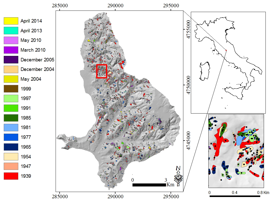
Figure 1Multi-temporal landslide inventory dating from 1939 to 2014 (left map; adapted from Samia et al., 2017a, b, 2018). Collazzone study area and Umbria region (right upper map). The coordinate system of maps is EPSG:32633 (https://www.spatialreference.org/). Landslide points were constructed by placing a point in the geometric centre of each landslide polygon (map in the right lower corner). The red rectangle shows the extent of the map in the lower right.
Statistically based landslide susceptibility techniques have been the preferred technique in the modelling of landslide susceptibility (Reichenbach et al., 2018). In statistical landslide susceptibility modelling, empirical quantitative relations are explored between the spatial distribution of landslides and a set of environmental factors (e.g., slope and geology; Van Westen et al., 2003; Guzzetti et al., 2005). The spatial distribution of historic landslides, documented in landslides inventories, is therefore a crucial input for statistically based landslide susceptibility modelling (Guzzetti et al., 2012; Van Westen et al., 2008). Direct field mapping, visual interpretation of aerial photographs and other remote-sensing images are the main sources for such mapping of landslide inventories (Guzzetti et al., 2012). Landslides in such inventories are stored as points or polygons. Although polygon-based landslide inventories (Ardizzone et al., 2018; Schlögel et al., 2011; Galli et al., 2008) are becoming increasingly available, in many landslide-prone regions, only less-detailed point-based landslide inventories are collected (Gorum et al., 2011; Sato et al., 2007; Keefer, 2000). Conditioning attributes used in landslide susceptibility modelling are mainly derivatives of digital elevation models (DEMs) along with geological, soil and land use data (Günther et al., 2014; Neuhäuser et al., 2012; Reichenbach et al., 2018). While geology, land use and soil data are not always available in high detail, DEM derivatives are easily computed and globally available at a range of resolutions. Therefore, the minimum available dataset for landslide susceptibility modelling includes a point-based landslide inventory and a set of DEM-derived conditioning attributes.
Traditionally, landslide susceptibility is considered time-invariant: susceptibility of a place to landslide occurrence is constant over time, at least over decadal scales. Recently, we proposed the concept of time-variant landslide susceptibility, where susceptibility changes over time due to the transient effect of previous landslides on future landslide occurrence (Samia et al., 2017a, b). We referred to such a transient effect as “path dependency”, a term adopted from complex system theory where it is used to describe the concept that the history of a system specifies the future behaviour of a system through legacy effects (Phillips, 2006). In our study area in Umbria, central Italy (Fig. 1), we identified the existence of path dependency among landslides: earlier landslides locally increased the susceptibility for future landslides for about 2 decades, during which the susceptibility decays exponentially over time (Samia et al., 2017b). We first implemented the effect of this landslide path dependency in landslide susceptibility modelling at the scale of slope units. Such units divide an area into hydrological units bounded by drainage and dividing lines (Carrara et al., 1991; Alvioli et al., 2016). We found that the impact of path dependency on landslide susceptibility models at the slope-unit scale was limited (Samia et al., 2018). This limited impact of landslide path dependency on model predictions was probably due to the fact that landslide path dependency affects landslide patterns at spatial scales smaller than slope units, and we hypothesized that differences between models were likely to increase when including path dependency at smaller spatial scales.
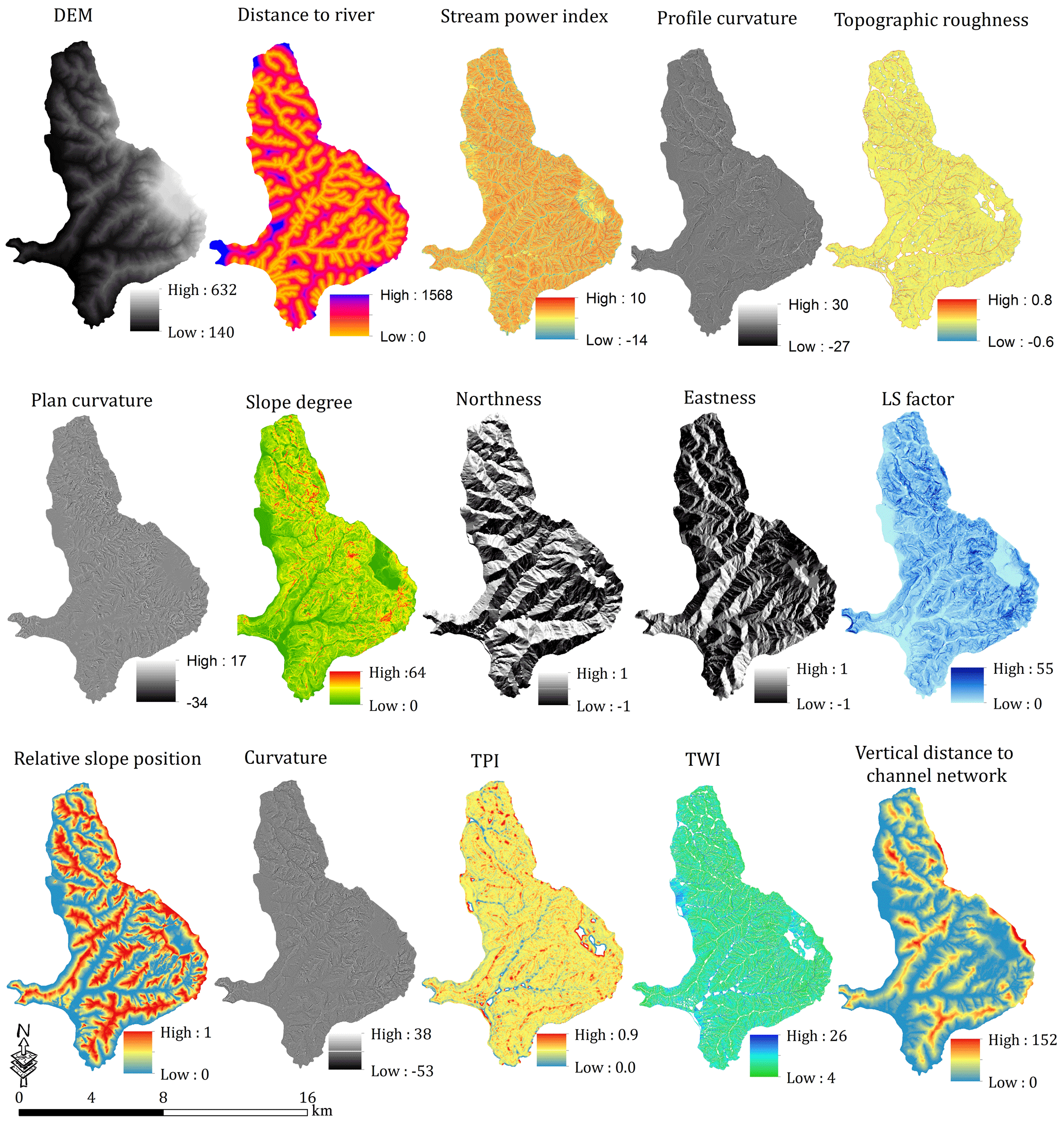
Figure 2DEM (digital elevation model) and its derivatives used in conventional and conventional plus path-dependent landslide susceptibility models. TPI means topographic position index, TWI means topographic wetness index, and LS factor stands for slope length and steepness factor.
The objective of this work is thus to consider the effect of landslide path dependency in landslide susceptibility modelling at the resolution of 10 m×10 m pixels. We hypothesize that including landslide path dependency will improve the performance of landslide susceptibility models. We also explore whether a purely path-dependent landslide susceptibility model, i.e., based solely on landslide inventory information, can provide a meaningful landslide susceptibility map. We use the unique multi-temporal landslide inventory from the Collazzone study area (Fig. 1; Guzzetti et al., 2006a; Ardizzone et al., 2007, 2013).
The Collazzone study area in Umbria, central Italy (Fig. 1), extends to about 80 km2, with a terrain elevation between 140 to 632 m and terrain slope derived from a 10 m×10 m DEM (Fig. 2) between 0 and 64∘. The DEM was prepared by interpolating 5 and 10 m contour lines shown in 1:10 000 topographic maps (Guzzetti et al., 2006b). A set of DEM derivatives that has been widely used in landslide susceptibility modelling was computed in SAGA GIS and ArcGIS. We expect that these DEM derivatives capture topographical, geomorphological and hydrological properties of locations in our study area.
The DEM derivatives (Fig. 2) are the slope angle, curvature, plan and profile curvature, aspect, northness and eastness as cosine and sine transformations of aspect, topographic position index (TPI) representing different geomorphological settings (Costanzo et al., 2012), stream power index (SPI) representing the erosive power of streams (Moore et al., 1993), and topographic wetness index (TWI) as an index for hydrological processes in the slope (Jebur et al., 2014). Additionally, for every pixel, we computed the distance to the nearest river, the slope length and steepness factor (LS factor) as an index for soil erosion on slope (Moore and Wilson, 1992), the vertical distance to the slope's channel network, and the relative slope position representing the relative position of slope in cells between the valley bottom and ridgetop. Additionally, we calculated topographic roughness, which expresses the difference in the values of elevation in the neighbouring cells in the DEM (Riley et al., 1999), and the standard deviation of elevation and slope in a 3 pixel×3 pixel window. These 16 DEM derivatives were used as independent explanatory variables in logistic regression for modelling of landslide susceptibility (see Sect. 3.2).
Landslides are abundant in this area and range from recent shallow landslides to old deep-seated landslides (Guzzetti et al., 2006a). Intense and prolonged rainfall and rapid snowmelt are the main triggers of landslides in the area (Cardinali et al., 2000; Ardizzone et al., 2007). A unique multi-temporal landslide inventory with 3391 landslides has been mapped in 19 different time slices. The age of the landslides ranges from relict and very old landslides with an uncertain date of occurrence to landslides that occurred in 2014. Aerial photographs, direct geomorphological field mapping and satellite images were used for the preparation of the multi-temporal landslide inventory (Ardizzone et al., 2013; Guzzetti et al., 2006a; Galli et al., 2008). Only time slices of the multi-temporal inventory for which the relative date of occurrence is known (Fig. 1) were used in this study because time between landslides is a key element in the quantification of landslide path dependency (Samia et al., 2017a, b). In addition, the first time slice, with the known date of 1939, was only used in the computation of the landslide path-dependency parameters and not in landslide susceptibility modelling because of its unknown past. Ultimately, a multi-temporal landslide inventory was used that contains the distribution of landslides in 16 time slices dating from 1947 to 2014 (Fig. 1). This multi-temporal landslide inventory was mostly prepared at the scale of 1:10 000, which is sufficient for conversion to a 10 m×10 m pixel-based landslide inventory. However, time slices from 1939 to 1997 were prepared from aerial photographs with scales ranging from 1:15 000 to 1:33 000, and this may introduce some positional inaccuracy in landslides of the order of one pixel. Given that the median size of landslides in this period is 19 pixels, we believe that this is an acceptable level of inaccuracy.
More information about the Collazzone study area and the multi-temporal landslide inventory is given in Galli et al. (2008), Guzzetti et al. (2006a, 2009) and Ardizzone et al. (2007).
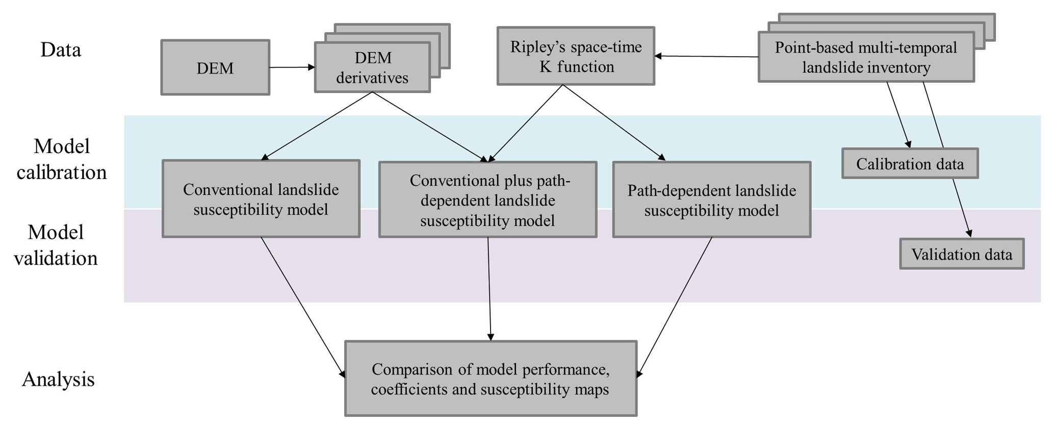
We used logistic regression to construct three different landslide susceptibility models (Fig. 3): (i) a conventional landslide susceptibility model using DEM derivatives, (ii) a conventional plus path-dependent landslide susceptibility model using 16 DEM derivatives and two landslide path-dependency variables (explained below), and (iii) a purely path-dependent landslide susceptibility model using only the two landslide path-dependency variables. We compared the performance of these models using area-under-the-curve (AUC) values from the receiver operating characteristic (ROC; Mason and Graham, 2002) and selected the optimal model using the Akaike information criterion (AIC; Akaike, 1998), which penalizes the use of additional variables in a model. Ultimately, the coefficients of the variables selected by three landslide susceptibility models and the resulting landslide susceptibility maps were compared.
3.1 Quantifying landslide path dependency using Ripley's space–time K function
The spatio-temporal dynamics of landslide path dependency was recently quantified for the Collazzone study area (Samia et al., 2017a) and was implemented in landslide susceptibility modelling at the scale of slope units (Samia et al., 2018). Our previous quantification of landslide path dependency used simplified information about the spatial overlap among landslides in a polygon-based multi-temporal landslide inventory (Samia et al., 2017b). The novel aspect of the present paper is that now, at finer spatial resolutions, we quantify landslide path dependence simultaneously in space and time. For this quantification, we use Ripley's K function (Ripley, 1976; Diggle et al., 1995). Ripley's K function has been used mainly in spatial point pattern analysis and reflects the degree of spatial clustering of events (e.g., landslides – Tonini et al., 2014; forest fires – Gavin et al., 2006; crimes – Levine, 2006; and disease outbreaks – Hinman et al., 2006). The function determines whether events are clustered, dispersed or randomly distributed. A modified Ripley's K function was also used to quantify the degree of clustering of point events in space and time (Lynch and Moorcroft, 2008; Ye et al., 2015). In the landslide path-dependency context, we used Ripley's space–time K function to reflect the degree to which landslides occur near previous landslides and how this changes with increasing distance to the previous landslide in space and time. The starting point to derive Ripley's K is a point-based multi-temporal landslide inventory consisting of points in the geometric centre of polygons of landslides (Fig. 1).
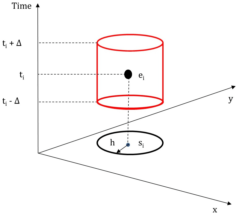
Ripley's space–time K function tests whether the number of events that is observed in a space–time cylinder around an initial event is equal to what is expected given the average point density in space and time (Ripley, 1976, 1977; Diggle et al., 1995). The space–time cylinder I(h,Δ) (Fig. 4) is defined as
where h shows the spatial distance increment, Δ shows the time increment, i and j are two landslide centre points, and d and t reflect the distance and time between the two landslide centre points, respectively.
The expected Ripley K function for one space–time cylinder of size h and Δ is defined as
where E is the expected number of landslides in the cylinder, and λst reflects the average space–time intensity of the landslides, i.e., the expected number of landslides per unit of space–time volume, which is calculated as
where n is the number of landslides in the entire inventory, t is time and a(R) reflects the size of the area. Therefore, the expected Ripley space–time K function for the space–time cylinders around each landslide point is defined as
Similarly, the observed Ripley space–time K function is calculated from the landslide inventory:
Finally, we defined the space–time clustering (STC) measure, which reflects how much more likely it is that a landslide will occur given a time and space distance from a previous landslide, as follows:
STC values > 0 indicate clustering, and values < 0 indicate dispersion. We calculated STC (h, Δ) for a wide range of h and Δ: values of h ranged from 0 to 500 m in 30 steps, and values of Δ ranged from 0 to 38 years in 30 steps. This yielded 900 empirical values of STC (h, Δ). We then fitted an exponential-decay function of h and Δ to the empirical STC values. This exponential-decay function was used to calculate STC values for each pixel, depending on when and where a landslide last occurred closely to that pixel.
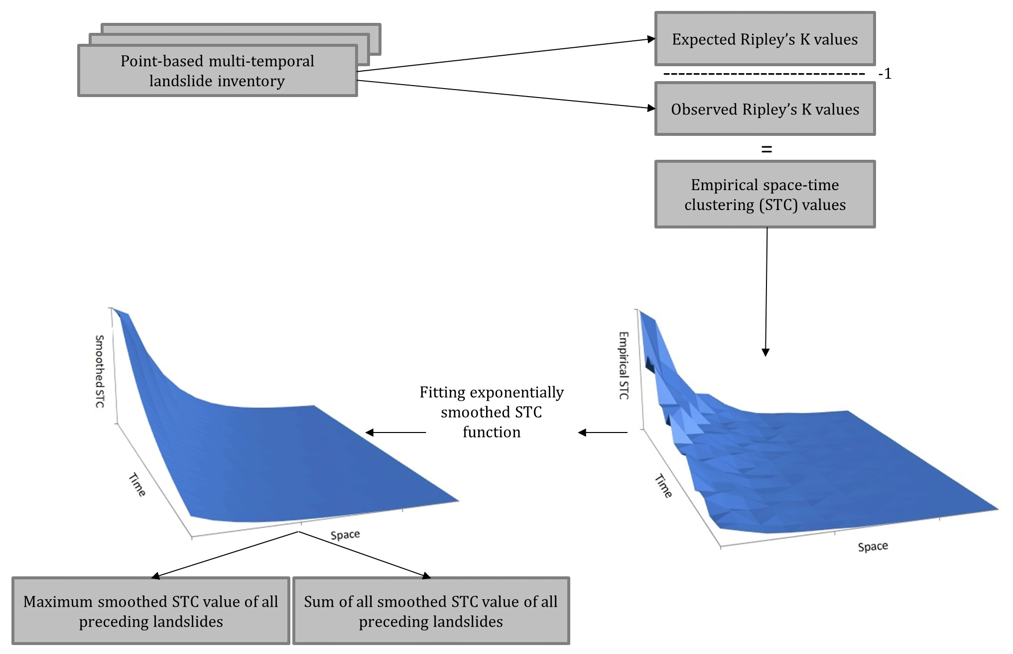
Figure 5Procedure to compute the two landslide path-dependency variables using Ripley's space–time K function.
Based on this, we calculated two landslide path-dependency variables (Fig. 5). The first variable reflects the maximum value of all STC values for all previous landslides near a pixel. This variable results in high values when one particular previous nearby landslide is expected to have a large impact on the susceptibility of landslides. The second variable is the sum of all STC values of all previous landslides near a pixel. This variable results in high values when all previous nearby landslides are expected to have a large impact on the susceptibility of landslides. This approach mirrors what we did in our slope-unit-based susceptibility model (Samia et al., 2018) in the sense that the variables separate the impact of the most impactful previous nearby landslide from the impacts of all previous nearby landslides.
3.2 Logistic regression
Logistic regression is considered a reference model in statistically based landslide susceptibility modelling (Reichenbach et al., 2018). Relations between presence and absence of landslides as a binary target variable are explained by a set of independent variables such as slope steepness and slope position in logistic regression. In this paper, DEM derivatives (Sect. 2 and Fig. 2) as well as the two landslide path-dependency variables computed using Ripley's space–time K function (see Sect. 3.1) were used as independent variables. Landslide presence or absence was the binary target variable.
3.3 Training and testing
When using a multi-temporal landslide inventory in landslide susceptibility modelling, the selection of time slices for the training and testing is crucial. In Rossi et al. (2010) and Samia et al. (2018), a sequential splitting sampling strategy was used in such a way that landslides in older time slices were used to train the model and landslides in newer time slices were used to test the model. However, such a sequential sampling strategy does not provide an equal range of landslide histories between training and testing datasets, and this could bias the role of time in path-dependent landslide susceptibility modelling. To avoid such a timing inequality, Samia et al. (2018) also introduced a non-sequential sampling strategy in which the span of timing segregation among time slices in the training and the testing datasets is comparable. In this study, we used this sampling strategy to split the multi-temporal landslide inventory into training and testing datasets. To achieve this, all landslides in the time slices of 1947, 1954, 1981, 1985, 1999, May 2004, and March and May 2010 were used for training, and all landslides in the time slices of 1965, 1977, 1991, 1997, December 2004 and 2005, and April 2013 and 2014 were used for testing (Fig. 1). It is important to note that the time slice in 1939 was used only for quantification of landslide history of the other time slices and not for training or testing. Thus, the first time slice in the training dataset is 1947 (Fig. 1).
The number of pixels with landslides was smaller than the number of pixels without landslides in both training and testing datasets. Therefore, we randomly selected 5000 pixels with landslides and 5000 pixels without landslides from both training and testing datasets in order to create equal datasets both for training and testing of the models. This random selection of pixels was repeated 10 times both in the training and testing datasets. Therefore, we trained the conventional, conventional plus path-dependent and purely path-dependent landslide susceptibility 10 times and later tested 10 times. After preparation of the 10 training datasets, logistic regression was applied to the 10 training datasets with an entry probability of 0.05 and removal probability of 0.06 for independent variables to diminish the chance of overfitting in the model. We only allowed inter-variable correlations of less than 0.8 to avoid multicollinearity. Conventional landslide susceptibility was modelled using DEM derivatives only once for the defined training dataset and was tested using the independent testing dataset. The conventional plus path-dependent landslide susceptibility model was constructed using DEM derivatives plus the two landslide path-dependency variables. The purely path-dependent landslide susceptibility was modelled only by using the two landslide path-dependency variables. All three models were constructed only once. Model performance was assessed using AUC and AIC values. The AUC values for testing were assessed using 10 training models and 10 independent testing datasets. The models with highest performance in terms of AUC values were used to map susceptibility to landslides. Finally, we compared landslide susceptibility maps resulting from conventional, conventional plus path-dependent and purely path-dependent susceptibility.
4.1 Spatio-temporal dynamic of landslide path dependency
Ripley's space–time K function confirmed the existence of landslide path dependency at small spatial and small temporal distances from a previous landslide (Fig. 6). The STC measure (Eq. 6) is high in the space–time vicinity of an earlier landslide, and it then decreases rapidly. Apparently, landslide susceptibility is relatively high immediately after occurrence of an earlier, nearby landslide.
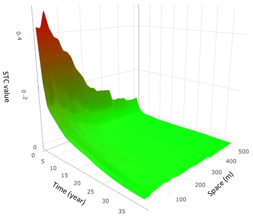
Figure 6Space–time dynamic of landslide path dependency. The colours represent the intensity of STC measure. Red indicates high STC, and green indicates low STC.
The exponential-decay function that was fitted to the empirical STC values is
This function shows that the STC measure decays exponentially over a characteristic timescale of 16.7 years and characteristic spatial scale of 58.8 m. The residual standard error of the exponential function is 0.01, in units of STC (–), which compares favourably with the actual values that range up to 0.44.
4.2 Model performance
We compared performance of the conventional, conventional plus path-dependent and purely path-dependent landslide susceptibility models, using AUC (greater is better) and AIC (lower is better) values as measure of performance (Table 1 and Fig. 7). The best-performing landslide susceptibility model was the conventional plus path-dependent model, both when expressed as AUC values and as AIC values (Table 1). The purely path-dependent landslide susceptibility model, constructed with only the two landslide path-dependency variables, performed better than the conventional landslide susceptibility model with its 16 DEM-derived variables.
Table 1Performance of the three landslide susceptibility models. The values of AUC represent the average AUC values in the 10 training and 10 testing datasets. The values of AIC represent the average AIC values in the 10 training datasets.

Table 2Selection of independent variables in conventional, conventional plus path-dependent and purely path-dependent landslide susceptibility modelling. Variables selected six or more times are shown. The numbers in brackets indicate how often variables were selected.
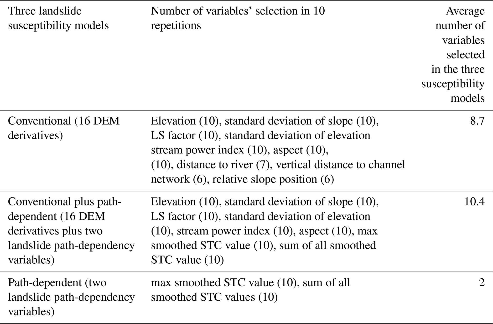
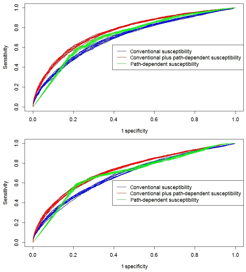
Figure 7Receiver operating characteristic (ROC) curves of the three landslide susceptibility models in the 10 training datasets (left) and in the 10 testing datasets.
For conventional susceptibility models, six DEM derivatives were selected in all 10 models (Table 2). Adding two landslide path-dependency variables into DEM derivatives variables affected the inclusion and exclusion of DEM-derivative variables only slightly. For example, the variables of TPI and distance to river were selected four and seven times, respectively, in the conventional susceptibility models, whereas after adding the two landslide path-dependency variables, these variables were selected five and four times, respectively. The variable eastness, which was selected twice in the conventional susceptibility models, was never selected in the conventional plus path-dependent susceptibility models.
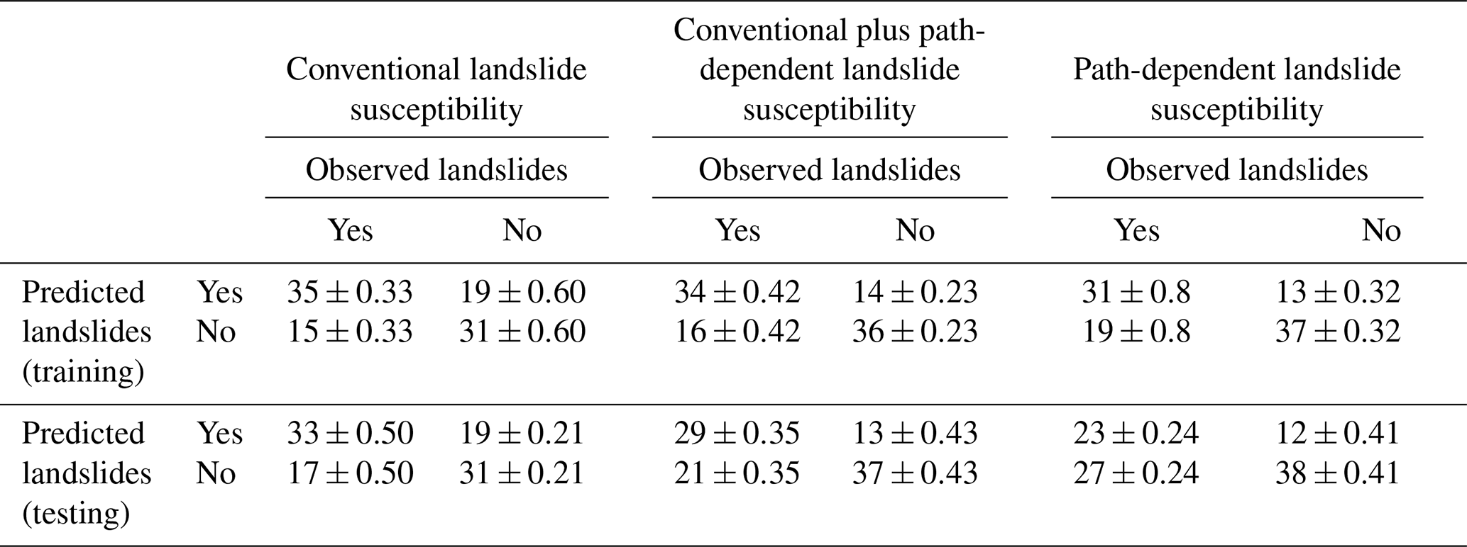
In all the training and the testing datasets, the contingency tables (Table 3) showed that conventional landslide susceptibility models differed substantially from the conventional plus path-dependent and path-dependent landslide susceptibility models. In particular, the percentage of false positives (the percentage of pixels without landslides predicted with landslides) for the conventional susceptibility models is higher than for the two other susceptibility models. However, there are also fewer true negatives (the percentage of pixels without landslides predicted without landslides) in the conventional than in the conventional plus path-dependent and path-dependent susceptibility models. The variation in the differences is larger in the training datasets than the testing datasets, suggesting that all fitted models are robust.
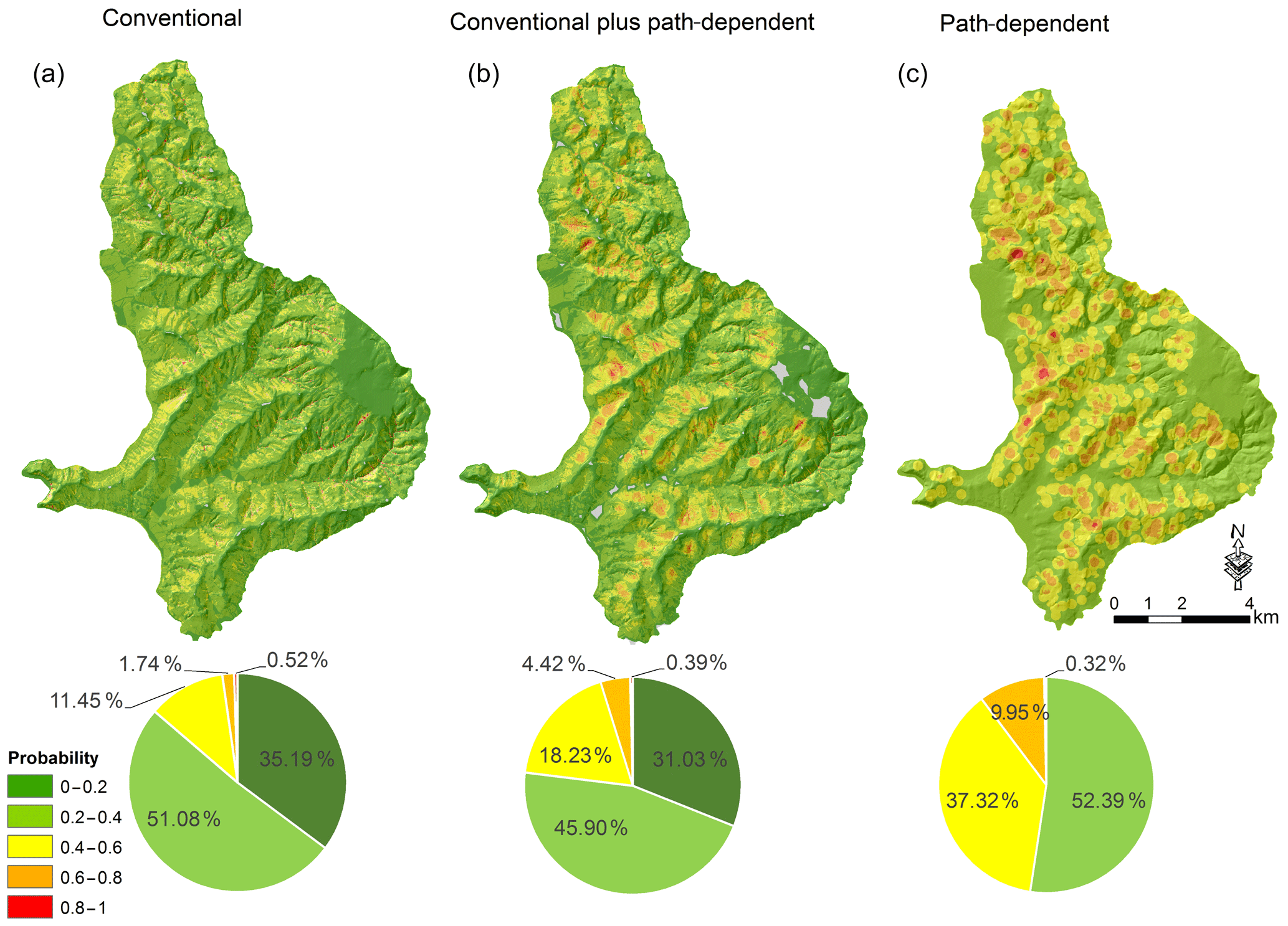
Figure 8Conventional landslide susceptibility map (a), the conventional plus path-dependent landslide susceptibility map (averaged out over 16 time slices) (b) and path-dependent landslide susceptibility map (averaged out over 16 time slices) (c). The pie charts show the percentage of pixels in each map in different probability levels of landslide occurrence.
Table 3Contingency tables computed with cut-off value of 0.5 for the three models. The numbers in the table represent the average values computed in the 10 training and 10 testing datasets.
4.3 Conventional, conventional plus path-dependent and purely path-dependent landslide susceptibility maps
The landslide susceptibility maps derived from the three models illustrate different patterns of landslide susceptibility (Fig. 8). For the models that include path dependency, the presented maps give the average values of all simulated time slices. Differences between the maps correspond with the considerable differences in the performance of their landslide susceptibility models in terms of AUC and AIC values (Table 1). The path-dependent landslide susceptibility map is visually different from both other landslide susceptibility maps, with the pattern dominated by regions of high susceptibility around locations where landslides previously occurred.
The 16 conventional plus path-dependent landslide susceptibility maps are dynamic and change over time (Fig. 9). These changes reflect the exponential decay with increasing time, since previous nearby landslides (Fig. 6) and the sudden increase in susceptibility in areas close to recent landslides. The gradual decrease in susceptibility levels is clearest when comparing the 1981 and 2004 susceptibility maps, whereas the sudden increase is clearest when comparing the 2004 and 2014 maps. The 2014 susceptibility map has higher susceptibility levels because of the impact of recent landslides in the year 2013.
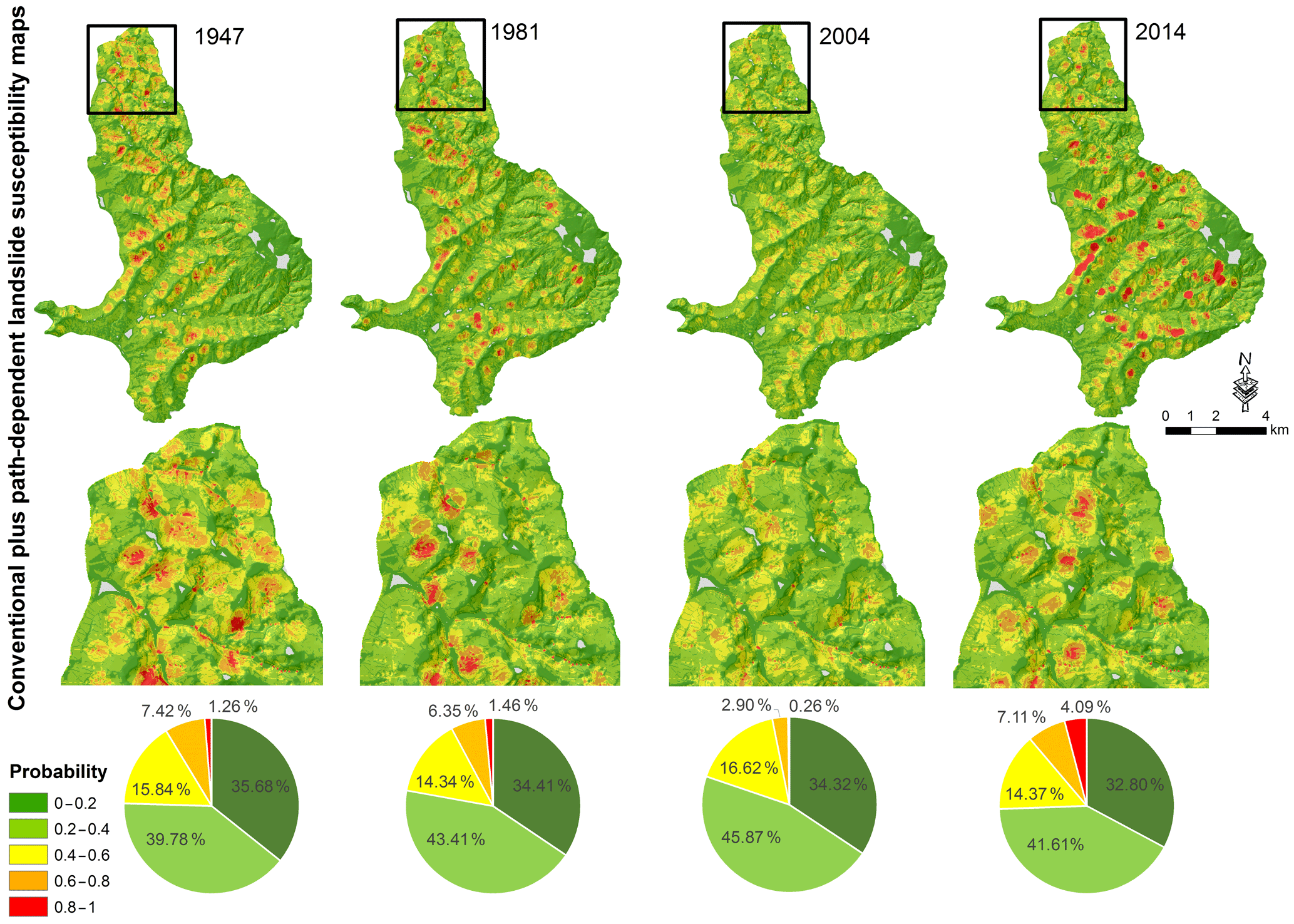
Figure 9Examples of four dynamic conventional plus path-dependent landslide susceptibility maps in the years 1947, 1981, 2004 and 2014. Zoomed maps show the places where there are large changes in susceptibility over time.
Similar dynamics are visible when comparing landslide susceptibility maps constructed with the purely path-dependent model for different years (Fig. 10). These maps show only the pure influence of earlier landslides on susceptibility to future landslides (Fig. 6). Again, the susceptibility of landslides decreases where distance from earlier landslides in space and time increases but jumps back up when more recent landslides become part of the landslide history. The pure influence of each individual landslide on the susceptibility to the future landslide is strong when a landslide is fresh, which is reflected in the high percentage of susceptibility levels of 0.6–0.8 and 0.8–1.0 in 1947 and 2014. As time passes since the previous landslide has occurred, the susceptibility decreases, with an exponential-decay response which is reflected in the low percentage of susceptibility levels of 0.6–0.8 and 0.8–1.0 in 1981 and 2004.
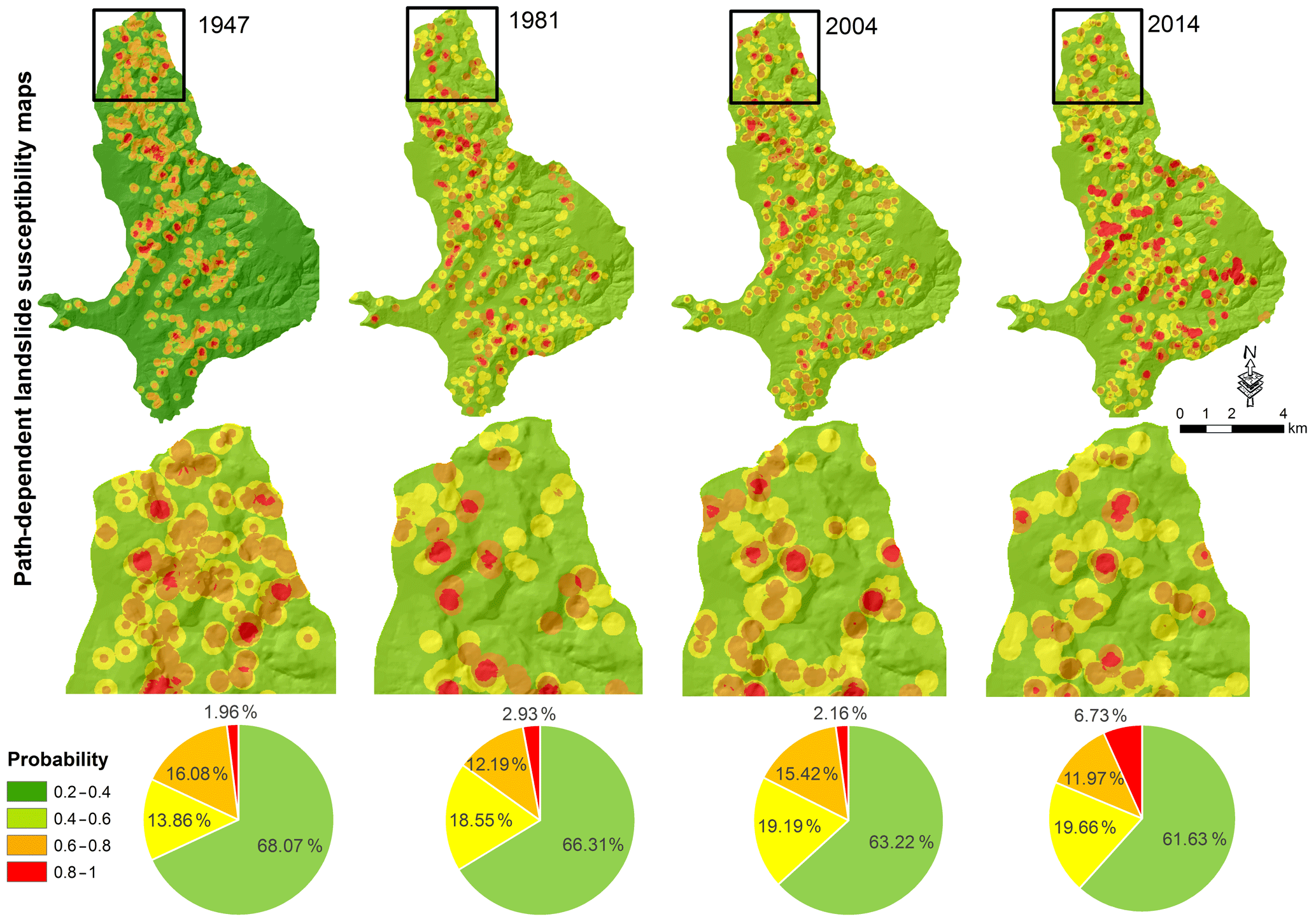
Figure 10Examples of four dynamic path-dependent landslide susceptibility maps in the years 1947, 1981, 2004 and 2014. Zoomed maps show the places where there are large changes in susceptibility over time.
In this section, we focus first on the quantification of landslide path dependency in the pixel-based multi-temporal landslide inventory and then discuss its role in susceptibility models. We also discuss the susceptibility model performance for all three model types. At the end, the exportability of landslide path-dependency parameters and the implication of dynamic time-variant path-dependent landslide susceptibility in landslide hazard are discussed.
5.1 Quantification of landslide path dependency
The quantification of landslide path dependency using Ripley's space–time K function (Ripley, 1976; Diggle et al., 1995) indicates, in our study area, an exponential-decay response in the STC values (Fig. 6). This means that there is a positive influence of earlier nearby landslides on susceptibility that decays exponentially in time and space with a characteristic timescale of about 17 years and a characteristic spatial scale of about 60 m. This is in accordance with our previously quantified landslide path dependency using a follow-up landslide fraction in which the decay period of landslide path dependency was found to be about 2 decades (Samia et al., 2017b). Landslide clustering manifests in the form of spatial association among landslides, where follow-up landslides occur immediately after and close to a previous landslide (Samia et al., 2017a). Samia et al. (2017b) discussed the possible mechanism in the formation of clusters of landslides in which the size of the initial landslide and changes in hydrology of slope destabilized by a landslide could facilitate the occurrence of follow-up landslides and hence clusters of landslides.
STC values and their exponential decay to some extent depend on the method that we have chosen to determine the centre point of landslides when converting polygons of landslides to points of landslides. Our approach was to take the geometric centre, but other options exist (Haines, 1994) and their impact should be explored. Also, in the computation of STC values with Ripley's space–time K function, distance between landslides was calculated using the Pythagorean theorem without distinguishing between distances in the x and y direction. Also we did not include differences in the elevation of centre points in our distance calculations. For future work, it could be interesting to define one dimension as the distance along the slope in the downslope direction and another dimension as the distance in the slope parallel direction, keeping these two spatial dimensions separate in addition to the temporal dimension.
5.2 Effect of landslide path dependency on performance of landslide susceptibility models
Our results demonstrated that including the landslide path-dependency effect in a pixel-based landslide susceptibility model constructed by DEM derivatives improves model performance substantially. This is in line with high AUC and low AIC values for the conventional plus path-dependent landslide susceptibility model (Table 1 and Fig. 7). This confirms our main hypothesis that adding the effect of landslide path dependency boosts the performance of landslide susceptibility models and is in accordance with our previous expectations regarding the stronger effect of landslide path dependency in a pixel-based landslide susceptibility model than in a slope-unit-based landslide susceptibility model (Samia et al., 2018). Landslide path dependency is a local effect (apparently with characteristic spatial scale of about 60 m) in which an earlier landslide increases the likelihood of follow-up landslide occurrence. Such a local effect is obviously more visible at pixel resolution of 10 m rather than at slope-unit resolution (with a median size of 51 486 m2 in our study area).
Strikingly, the purely path-dependent landslide susceptibility model constructed with only the two landslide path-dependency variables performs better than the conventional landslide susceptibility model made by DEM-derivative variables (Table 1 and Fig. 7). This is potentially interesting, since it implies that the landslide inventory itself can be used to map susceptibility to landslides without using DEM derivatives which have been conventionally used in landslide susceptibility modelling (Varnes, 1984; Guzzetti et al., 2005). The performance of this path-dependency-only model thus highlights that proximity to previous landslides can adequately capture susceptible locations. It also suggests that the path-dependent models' success in our experiments may be partly due to the fact that they capture static spatial effects that have not been resolved with our explanatory factors. It is attractive to imagine follow-up work that attempts to disentangle this static spatial effect that is unrelated to landslide history from dynamic spatial effects that are related to landslide history. The key to such disentangling should be that the former does not decay over time, whereas the latter does. More advanced statistical approaches that simultaneously estimate purely spatial and spatio-temporal effects may be needed. More complex explanatory variables such as geology, soil and land use can also be used along with DEM derivatives to improve landslide susceptibility models and maps. However, these are not always available. In fact, considering the landslide path-dependency effect in such complete explanatory factors improves their performance as well. We confirmed this in an additional exploration where we constructed a conventional landslide susceptibility model used in this paper, with the same DEM derivatives but also with land use and geology as explanatory factors. The results demonstrated that adding our two landslide path-dependency variables to such an improved conventional landslide susceptibility increased its performance (from an AUC value of 0.771 to an AUC value of 0.801).
Another important aspect of considering the landslide path-dependency effect in landslide susceptibility modelling is providing dynamic landslide susceptibility maps. Landslide susceptibility maps are usually classified into five levels of probability of landslide occurrence, ranging from 0 to 1. In the conventional landslide susceptibility map (Fig. 8a), the five probability levels of susceptibility by definition remain constant over time, since the DEM derivatives in the model are constant (although DEM derivatives also change when a landslide occurs, but DEMs are not updated frequently enough to reflect this). The usage of conventional static landslide susceptibility maps and dynamic landslide susceptibility maps taking landslide path dependency depends on the goal and task of audience. In reality, static susceptibility maps created (either with a conventional susceptibility model or as the static portion of a conventional plus path-dependent model) can be used in sustainable planning, whereas dynamic susceptibility maps can be considered in short-term land use planning.
However, adding landslide path dependency in landslide susceptibility models provides dynamic landslide susceptibility maps (Figs. 9 and 10) in which the levels of susceptibility change over time, reflecting the exponential-decay response of landslide path dependency (Fig. 6). The changes are in the places where landslides have already occurred, mainly in probability levels of susceptibility, ranging from 0.6 to 1.0. This suggests that the part of the area located in the high-probability level of susceptibility could switch to the low-probability level of susceptibility (0 to 0.6) after a decade. This is exemplified between the 1947 and 1954 landslide susceptibility maps, in which about 9 km2 of the study area drops by more than 0.1 in its probability of landslide occurrence. After adding the two path-dependency variables in the conventional landslide susceptibility modelled with DEM derivatives, it turns out that the coefficients of all DEM-derivative variables become lower (e.g., the LS factor becomes less important).
5.3 Can landslide path-dependency parameters be transported to other areas?
In landslide-prone areas where landslides are documented and mapped in the form of polygon-based multi-temporal inventories, the landslide path dependency can be quantified based on geographical overlap among landslides and hence used in landslide susceptibility modelling (Samia et al., 2017b, 2018). However, polygon-based multi-temporal landslide inventories are rare to the best of our knowledge, and hence in many areas geographical overlap among landslides cannot be computed. In this paper, we proposed using Ripley's space–time K function to compute landslide path dependency where point-based multi-temporal landslide inventories are used. Using such inventories, our STC measure (Eq. 6) can be used to quantify path dependency among landslides.
It is attractive to think that the STC measure (Eq. 6) and its parameters (Eq. 7) can be directly exported to landslide-prone areas with substantial geological and topographical similarities. However, to gain confidence in this approach, multi-temporal landslide inventories from such places (e.g., Schlögel et al., 2011) need to be questioned to find out whether path dependency occurs, whether it occurs over a similar space and timescales, and whether it adds value to susceptibility modelling. This would also allow us to start exploring what determines the characteristic space and timescales.
5.4 Implications of path-dependent landslide susceptibility in landslide hazard assessment
We have already modified the definition of conventional landslide susceptibility modelling (Varnes, 1984; Guzzetti et al., 2005) using spatial temporal dynamics of landslide path dependency (Samia et al., 2017a, b) as follows:
In this study, both conventional plus path-dependent and path-dependent landslide susceptibility models turned out to perform better than a conventional landslide susceptibility model (Table 1 and Fig. 7). In both models, availability of a space–time component – reflecting the exponential decay of landslide path dependency – indicates that landslide susceptibility is dynamic. This challenges the way in which landslide hazard is assessed, as landslide susceptibility is an important element of landslide hazard.
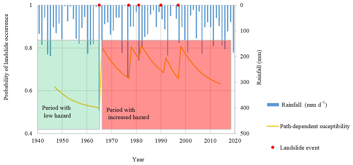
Figure 11Conceptual model of the implication of dynamic path-dependent landslide susceptibility model in landslide hazard assessment. When susceptibility is low, the hazard is also low (providing the other components of landslide hazard, e.g., size, remain unchanged) and large rainfall events are needed to trigger new landslides. Then, when susceptibility is raised by such landslides, the hazard is also high and small rainfall events may trigger new landslides.
In landslide hazard assessment, landslide susceptibility as a proxy of “where landslides occur” is combined with the temporal probability of landslide triggers (mainly rainfall) to determine “when landslides occur” (Guzzetti et al., 2006a). In this context, dynamic landslide susceptibility (Eq. 8) needs to be considered in combination with the temporal information of landslide triggers in the assessment of landslide hazard. When substantial landslides happen during a rainfall event, susceptibility in and around such landslides can be raised for a few decades in which moderate rainfall events may already cause substantial landslides, which raises susceptibility levels again (Fig. 11). Such dynamics have been observed in a site near Seattle, Washington, where several new landslides occurred in a slope that had recently experienced landslide activity, whereas a nearby hillslope with the same characteristics but without recently landslide activity did not experience new landslides (Mirus et al., 2017). If no substantial triggering event happens over the characteristic timescale of roughly 17 years, the increased susceptibility will be substantially reduced, and a later rainfall event may have less influence on landslides; the probability of experiencing a follow-up landslide will have decreased.
In the Collazzone study area, in central Italy, quantification of landslide path dependency reveals an exponential-decay response in landslide susceptibility as a function of spatio-temporal distance to earlier nearby landslides. For our study area, the characteristic timescale of this effect is about 17 years, and the characteristic spatial scale is about 60 m. Adding such an exponential-decay response of landslide path dependency in conventional pixel-based landslide susceptibility modelled by DEM derivatives improves the performance of model substantially. Taking into account landslide path-dependency effects in landslide susceptibility results in dynamic landslide susceptibility models where susceptibility changes over time. We stress that landslide susceptibility modelling should take the effect of landslide path dependency into account, since it provides an estimation of the temporal validation of different probability levels of landslide occurrence in a landslide susceptibility map. The obtained landslide path-dependency parameters can possibly be used for dynamic landslide susceptibility modelling in landslide-prone areas with environmental and data similarities. We proposed a conceptual model that considers the impact of dynamic path-dependent landslide susceptibility on landslide hazard.
The multi-temporal landslide inventory, DEM, and geological and land use data of the Collazzone study area in Italy were provided by CNR IRPI and can be requested from Fausto Guzzetti and Francesca Ardizzone. The code for analysis of Ripley's space–time K function can be requested from Jalal Samia and Arnaud Temme.
JS formulated the objective; designed the methodology; and conducted the GIS, statistical, and space–time Ripley analysis and modelling of landslide susceptibility. AT provided methodological support, advise and also major revisions to the paper. AB and JW made major revisions to the paper. FG and FA provided the data and also made major revisions to the paper.
The authors declare that they have no conflict of interest.
This research is part of Jalal Samia's PhD project at Wageningen University & Research, funded by the Ministry of Science, Research and Technology of Iran and the Laboratory of Geo-Information Science and Remote Sensing and Soil Geography and Landscape Group of Wageningen University and supported by the Geography Department of Kansas State University in the USA. The authors would like to thank Ben Mirus, the anonymous reviewer and also the editor Thomas Glade for their constructive comments and valuable suggestions, which have greatly improved the quality of the paper.
This research has been supported by the Ministry of Science Research and Technology of Iran (grant no. 104380) and the Wageningen University & Research (grant no. WUR2421E/247081).
This paper was edited by Thomas Glade and reviewed by Ben Mirus and one anonymous referee.
Akaike, H.: Information theory and an extension of the maximum likelihood principle, in: Selected Papers of Hirotugu Akaike, Springer, New York, 199–213, 1998.
Alvioli, M., Marchesini, I., Reichenbach, P., Rossi, M., Ardizzone, F., Fiorucci, F., and Guzzetti, F.: Automatic delineation of geomorphological slope units with r.slopeunits v1.0 and their optimization for landslide susceptibility modeling, Geosci. Model Dev., 9, 3975–3991, https://doi.org/10.5194/gmd-9-3975-2016, 2016.
Ardizzone, F., Cardinali, M., Galli, M., Guzzetti, F., and Reichenbach, P.: Identification and mapping of recent rainfall-induced landslides using elevation data collected by airborne Lidar, Nat. Hazards Earth Syst. Sci., 7, 637–650, https://doi.org/10.5194/nhess-7-637-2007, 2007.
Ardizzone, F., Fiorucci, F., Santangelo, M., Cardinali, M., Mondini, A. C., Rossi, M., Reichenbach, P., and Guzzetti, F.: Very-high resolution stereoscopic satellite images for landslide mapping, in: Landslide science and practice, Springer, Berlin, Heidelberg, 95–101, 2013.
Ardizzone, F., Fiorucci, F., Mondini, A. C., and Guzzetti, F.: TXT-tool 1.039-1.1: Very-High Resolution Stereo Satellite Images for Landslide Mapping, in: Landslide Dynamics: ISDR-ICL Landslide Interactive Teaching Tools: Volume 1: Fundamentals, Mapping and Monitoring, edited by: Sassa, K., Guzzetti, F., Yamagishi, H., Arbanas, Ž., Casagli, N., McSaveney, M., and Dang, K., Springer International Publishing, Cham, 83–94, 2018.
Brabb, E. E.: Innovative approaches to landslide hazard and risk mapping, in: International Landslide Symposium Proceedings, Toronto, Canada, 17–22, 1985.
Cardinali, M., Ardizzone, F., Galli, M., Guzzetti, F., and Reichenbach, P.: Landslides triggered by rapid snow melting: the December 1996–January 1997 event in Central Italy, in: Proceedings 1st Plinius Conference on Mediterranean Storms, 14–16 October 1999, Maratea, 439–448, 2000.
Carrara, A., Cardinali, M., Detti, R., Guzzetti, F., Pasqui, V., and Reichenbach, P.: GIS techniques and statistical models in evaluating landslide hazard, Earth Surf. Proc. Land., 16, 427–445, 1991.
Costanzo, D., Rotigliano, E., Irigaray, C., Jiménez-Perálvarez, J. D., and Chacón, J.: Factors selection in landslide susceptibility modelling on large scale following the gis matrix method: application to the river Beiro basin (Spain), Nat. Hazards Earth Syst. Sci., 12, 327–340, https://doi.org/10.5194/nhess-12-327-2012, 2012.
Diggle, P. J., Chetwynd, A. G., Häggkvist, R., and Morris, S. E.: Second-order analysis of space-time clustering, Stat. Meth. Med. Res., 4, 124–136, 1995.
Galli, M., Ardizzone, F., Cardinali, M., Guzzetti, F., and Reichenbach, P.: Comparing landslide inventory maps, Geomorphology, 94, 268–289, 2008.
Gavin, D. G., Hu, F. S., Lertzman, K., and Corbett, P.: Weak Climatic Control of Stand-Scale Fire History During The Late Holocene, Ecology, 87, 1722–1732, 2006.
Gorum, T., Fan, X., van Westen, C. J., Huang, R. Q., Xu, Q., Tang, C., and Wang, G.: Distribution pattern of earthquake-induced landslides triggered by the 12 May 2008 Wenchuan earthquake, Geomorphology, 133, 152–167, https://doi.org/10.1016/j.geomorph.2010.12.030, 2011.
Günther, A., Van Den Eeckhaut, M., Malet, J.-P., Reichenbach, P., and Hervás, J.: Climate-physiographically differentiated Pan-European landslide susceptibility assessment using spatial multi-criteria evaluation and transnational landslide information, Geomorphology, 224, 69–85, https://doi.org/10.1016/j.geomorph.2014.07.011, 2014.
Guzzetti, F., Reichenbach, P., Cardinali, M., Galli, M., and Ardizzone, F.: Probabilistic landslide hazard assessment at the basin scale, Geomorphology, 72, 272–299, 2005.
Guzzetti, F., Galli, M., Reichenbach, P., Ardizzone, F., and Cardinali, M.: Landslide hazard assessment in the Collazzone area, Umbria, Central Italy, Nat. Hazards Earth Syst. Sci., 6, 115–131, https://doi.org/10.5194/nhess-6-115-2006, 2006a.
Guzzetti, F., Reichenbach, P., Ardizzone, F., Cardinali, M., and Galli, M.: Estimating the quality of landslide susceptibility models, Geomorphology, 81, 166–184, https://doi.org/10.1016/j.geomorph.2006.04.007, 2006b.
Guzzetti, F., Ardizzone, F., Cardinali, M., Rossi, M., and Valigi, D.: Landslide volumes and landslide mobilization rates in Umbria, central Italy, Earth Planet. Sc. Lett., 279, 222–229, https://doi.org/10.1016/j.epsl.2009.01.005, 2009.
Guzzetti, F., Mondini, A. C., Cardinali, M., Fiorucci, F., Santangelo, M., and Chang, K.-T.: Landslide inventory maps: New tools for an old problem, Earth-Sci. Rev., 112, 42–66, 2012.
Haines, E.: Point in polygon strategies, Graphics gems IV, 994, 24–26, 1994.
Hinman, S. E., Blackburn, J. K., and Curtis, A.: Spatial and temporal structure of typhoid outbreaks in Washington, DC, 1906–1909: evaluating local clustering with the G i* statistic, Int. J. Health Geogr., 5, 13, 2006.
Jebur, M. N., Pradhan, B., and Tehrany, M. S.: Optimization of landslide conditioning factors using very high-resolution airborne laser scanning (LiDAR) data at catchment scale, Remote Sens. Environ., 152, 150–165, 2014.
Keefer, D. K.: Statistical analysis of an earthquake-induced landslide distribution – the 1989 Loma Prieta, California event, Eng. Geol., 58, 231–249, https://doi.org/10.1016/S0013-7952(00)00037-5, 2000.
Levine, N.: Crime mapping and the Crimestat program, Geogr. Anal., 38, 41–56, 2006.
Lynch, H. J. and Moorcroft, P. R.: A spatiotemporal Ripley's K-function to analyze interactions between spruce budworm and fire in British Columbia, Canada, Can. J. Forest Res., 38, 3112–3119, 2008.
Mason, S. J. and Graham, N. E.: Areas beneath the relative operating characteristics (ROC) and relative operating levels (ROL) curves: Statistical significance and interpretation, Q. J. Roy. Meteorol. Soc., 128, 2145–2166, 2002.
Mirus, B. B., Smith, J. B., and Baum, R. L.: Hydrologic Impacts of Landslide Disturbances: Implications for Remobilization and Hazard Persistence, Water Resour. Res., 53, 8250–8265, https://doi.org/10.1002/2017wr020842, 2017.
Moore, I. D. and Wilson, J. P.: Length-slope factors for the Revised Universal Soil Loss Equation: Simplified method of estimation, J. Soil Water Conserv., 47, 423–428, 1992.
Moore, I. D., Gessler, P., Nielsen, G., and Peterson, G.: Soil attribute prediction using terrain analysis, Soil Sci. Soc. Am. J., 57, 443–452, 1993.
Neuhäuser, B., Damm, B., and Terhorst, B.: GIS-based assessment of landslide susceptibility on the base of the weights-of-evidence model, Landslides, 9, 511–528, 2012.
Phillips, J. D.: Evolutionary geomorphology: thresholds and nonlinearity in landform response to environmental change, Hydrol. Earth Syst. Sci., 10, 731–742, https://doi.org/10.5194/hess-10-731-2006, 2006.
Reichenbach, P., Rossi, M., Malamud, B. D., Mihir, M., and Guzzetti, F.: A review of statistically-based landslide susceptibility models, Earth-Sci. Rev., 180, 60–91, https://doi.org/10.1016/j.earscirev.2018.03.001, 2018.
Riley, S. J., DeGloria, S., and Elliot, R.: Index that quantifies topographic heterogeneity, Intermount. J. Sci., 5, 23–27, 1999.
Ripley, B. D.: The second-order analysis of stationary point processes, J. Applied Probabil., 13, 255–266, 1976.
Ripley, B. D.: Modelling spatial patterns, J. Roy. Stat. Soc. B, 172–212, 1977.
Rossi, M., Guzzetti, F., Reichenbach, P., Mondini, A. C., and Peruccacci, S.: Optimal landslide susceptibility zonation based on multiple forecasts, Geomorphology, 114, 129–142, https://doi.org/10.1016/j.geomorph.2009.06.020, 2010.
Samia, J., Temme, A., Bregt, A., Wallinga, J., Guzzetti, F., Ardizzone, F., and Rossi, M.: Do landslides follow landslides? Insights in path dependency from a multi-temporal landslide inventory, Landslides, 14, 547–558, https://doi.org/10.1007/s10346-016-0739-x, 2017a.
Samia, J., Temme, A., Bregt, A., Wallinga, J., Guzzetti, F., Ardizzone, F., and Rossi, M.: Characterization and quantification of path dependency in landslide susceptibility, Geomorphology, 292, 16–24, https://doi.org/10.1016/j.geomorph.2017.04.039, 2017b.
Samia, J., Temme, A., Bregt, A. K., Wallinga, J., Stuiver, J., Guzzetti, F., Ardizzone, F., and Rossi, M.: Implementing landslide path dependency in landslide susceptibility modelling, Landslides, 15, 2129–2144, 2018.
Sato, H. P., Hasegawa, H., Fujiwara, S., Tobita, M., Koarai, M., Une, H., and Iwahashi, J.: Interpretation of landslide distribution triggered by the 2005 Northern Pakistan earthquake using SPOT 5 imagery, Landslides, 4, 113–122, https://doi.org/10.1007/s10346-006-0069-5, 2007.
Schlögel, R., Torgoev, I., De Marneffe, C., and Havenith, H. B.: Evidence of a changing size–frequency distribution of landslides in the Kyrgyz Tien Shan, Central Asia, Earth Surf. Proc. Land., 36, 1658–1669, 2011.
Smith, T.: Notebook on spatial data analysis, Lecture Note, University of Pennsylvania, available at: http://www.seas.upenn.edu/~ese502/#notebook (last access: January 2020) , 2016.
Tonini, M., Pedrazzini, A., Penna, I., and Jaboyedoff, M.: Spatial pattern of landslides in Swiss Rhone Valley, Natural Hazards, 73, 97-110, 2014.
Van Westen, C. J., Rengers, N., and Soeters, R.: Use of geomorphological information in indirect landslide susceptibility assessment, Nat. Hazards, 30, 399–419, 2003.
Van Westen, C. J., Castellanos, E., and Kuriakose, S. L.: Spatial data for landslide susceptibility, hazard, and vulnerability assessment: an overview, Eng. Geol., 102, 112–131, 2008.
Varnes, D. J.: Landslide hazard zonation: a review of principles and practice, UNESCO, Paris, 1984.
Ye, X., Xu, X., Lee, J., Zhu, X., and Wu, L.: Space–time interaction of residential burglaries in Wuhan, China, Appl. Geogr., 60, 210–216, https://doi.org/10.1016/j.apgeog.2014.11.022, 2015.