the Creative Commons Attribution 4.0 License.
the Creative Commons Attribution 4.0 License.
 | 10 Oct 2020
Multivariate statistical modelling of the drivers of compound flood events in south Florida
Robert Jane
Luis Cadavid
Jayantha Obeysekera
Thomas Wahl
Miami-Dade County (south-east Florida) is among the most vulnerable regions to sea level rise in the United States, due to a variety of natural and human factors. The co-occurrence of multiple, often statistically dependent flooding drivers – termed compound events – typically exacerbates impacts compared with their isolated occurrence. Ignoring dependencies between the drivers will potentially lead to underestimation of flood risk and under-design of flood defence structures. In Miami-Dade County water control structures were designed assuming full dependence between rainfall and Ocean-side Water Level (O-sWL), a conservative assumption inducing large safety factors. Here, an analysis of the dependence between the principal flooding drivers over a range of lags at three locations across the county is carried out. A two-dimensional analysis of rainfall and O-sWL showed that the magnitude of the conservative assumption in the original design is highly sensitive to the regional sea level rise projection considered. Finally, the vine copula and Heffernan and Tawn (2004) models are shown to outperform five standard higher-dimensional copulas in capturing the dependence between the principal drivers of compound flooding: rainfall, O-sWL, and groundwater level. The work represents a first step towards the development of a new framework capable of capturing dependencies between different flood drivers that could potentially be incorporated into future Flood Protection Level of Service (FPLOS) assessments for coastal water control structures.
- Article
(2312 KB) - Full-text XML
-
Supplement
(4454 KB) - BibTeX
- EndNote


Florida is more vulnerable to sea level rise (SLR) in terms of housing and population relative to local mean high-tide levels than any other state in the country (Strauss et al., 2012). Miami-Dade County, located in the south-east of Florida, is particularly vulnerable due to its gently sloped low-lying topography, densely populated coastal areas, and economic importance (Zhang, 2011). Miami, the county's principal metropolitan area, is consistently ranked among the world's most exposed and vulnerable cities to coastal flooding (e.g. Hallegatte et al., 2013; Kulp and Strauss, 2017). While debate surrounds the region's vertical land motion (Parkinson and Donoghue, 2010), the contribution of SLR to nuisance or tidal flooding (Wdowinski et al., 2016) as well as its role in escalating socio-economic impacts such as climate gentrification is becoming increasingly apparent (Keenan et al., 2018). The future rates of SLR in the region are expected to be greater than the global average due to variations in the Florida Current and Gulf Stream (Southeast Florida Regional Climate Change Compact, 2015). Higher baseline ocean levels allow storm surges to propagate further inland whilst also reducing pressure gradients in rivers hampering efficient drainage; hence, SLR also increases the fluvial flood potential (Schedel et al., 2018).
In low-lying coastal areas flooding arises because of the interplay between metrological, hydrological, and oceanographic drivers including rainfall, river discharge, groundwater table, storm surge, and waves. In Miami Beach, for instance, Wdowinski et al. (2016) found that most flooding events between 1998 and 2013 occurred after heavy rain (> 80 mm) during high-tide conditions. The co-occurrence of multiple drivers can exacerbate the impacts of a flood and, depending on the adopted definition, be classified as a compound event (Seneviratne et. al., 2012; Leonard et al., 2014; Zscheischler et al., 2018). For example, significant statistical dependence between heavy rainfall and storm surge (or storm tide) has been identified over a range of spatial scales: global (Bevaqua et al., 2019), continental (Zheng et al., 2013; Wahl et al., 2015; Paprotny et al., 2018; Wu et al., 2018), regional to national (Svensson and Jones, 2002, 2004, 2006; Hendry et al., 2019), and local (Hawkes et al., 2002; Hawkes, 2008; White, 2009; van den Hurk, 2015; Lian et al., 2013; Zheng et al., 2014; Bengtsson, 2016). The dependence may arise due to common meteorological forcing (Pugh, 1987), potentially enhanced through orographic effects (Svensson and Jones, 2002, 2004; Martius et al., 2016), or simply by chance (Kew et al., 2013; Martius et al., 2016; Couasnon et al., 2019). Neglecting even weak dependence can result in the underestimation of water levels (Kew et al., 2013; Zheng et al., 2014; Ikeuchi et al., 2017) and consequently flood risk estimates (Lian et al., 2013; Zheng et al., 2013) in estuarine and tidal channels.
Miami-Dade County is underlined by the highly transmissive and porous (predominantly limestone) Biscayne aquifer, which is also the region's main source of potable freshwater (Randazzo and Jones, 1997). The lateral intrusion of saltwater into the unconfined aquifer as a recirculating saltwater wedge is widely acknowledged (Provost et al., 2018). SLR along with an increased likelihood of recurring drought during the winter–spring season, associated with changes in the climate system, enhances the risk of contamination of the water supply (Bloetscher et al., 2011). Furthermore, the county's population is expected to increase by nearly 20 % in the next 20 years (Florida Office of Economic and Demographic Research, 2015), increasing flood exposure and demand on water resources. The South Florida Water Management District (SFWMD) is responsible for managing and protecting the water resources of south Florida. The SFWMD must balance demand for potable water and agricultural and landscape irrigation with flood mitigation, whilst ensuring the water table remains sufficiently high to prevent saltwater intrusion and achieve other ecological objectives (SFWMD, 2016). Their aim is to meet these objectives through the continuous operation of an extensive network of drainage canals, storage areas, pumps, and other control structures. The Biscayne aquifer has a direct hydraulic connection to the natural and man-made surface water bodies, a consequence of its shallow depth and high porosity, and is therefore considered a part of this integrated hydrologic system (Randazzo and Jones, 1997).
In heavily managed urbanized catchments, antecedent groundwater conditions are an essential initial condition for hydraulic–hydrological models for robust flood risk analysis (Hettiarachchi et al., 2019). Rainfall is often employed as a surrogate for river discharge (e.g. Zheng et al., 2013; Wahl et al., 2015; Bevacqua et al., 2020). Physical properties such as the size, gradient, and permeability of a catchment influence the river response to a given rainfall event (Svensson and Jones, 2002; Zheng et al., 2013; Hendry et al., 2019). Verhoest et al. (2010) demonstrated that the return period of a rainfall event may differ significantly from that of the corresponding discharge, depending on the antecedent wetness of a catchment. In south-east Florida, approximately half of the average annual rainfall is lost to evapotranspiration (Bloetscher et al., 2011); hence rainfall is unlikely to constitute a suitable proxy for discharge.
Due to the unusually high connectivity of ground and surface water hydrology, south-east Florida has a high propensity for pluvial flooding. The concurrence of heavy precipitation and high antecedent soil moisture is the dominant flood-generating mechanism for most catchments without significant snowmelt (Berghuijs et al., 2016, 2019). Many recent studies (Moftakahri et al., 2017, 2019; Bevaqua et al., 2017; Couasnon et al., 2018, 2019; Paprotny et al., 2018; Ward et al., 2018; Serafin et al., 2019) statistically model river discharge and surge (or coastal water level in the case of Ganguli and Merz, 2019), or their relevant proxies (Kew et al., 2013), as opposed to rainfall and surge, implicitly accounting for catchment properties and pre-existing groundwater level (Lamb et al., 2010). Not accounting for groundwater level explicitly, especially in areas like Miami-Dade County where groundwater levels are highly responsive (and potentially correlated) to rainfall and O-sWL, precludes a robust assessment of the risk of pluvial flooding. Therefore, in this work, statistical models will be tested for their ability to capture the joint probability distribution of rainfall, O-sWL (tide + non-tidal residual), and groundwater level.
Traditional multivariate probability distributions are often restrictive in terms of the choice of marginal distributions; i.e. all the margins are required to be the same type of distribution. For example, fitting a bivariate Gaussian distribution to extreme tides and corresponding freshwater flows required Loganathan et al. (1987) to assume Gaussian marginal distributions. Copulas allow the dependence and marginal modelling to be carried out independently, providing more flexibility in the choice of marginal distributions than traditional multivariate models (Patton, 2006). Consequently, bivariate copulas have been used extensively in the modelling of compound flooding induced by rainfall and surge (e.g. Wahl et al., 2015) and from discharge in multiple rivers at their confluences (Wang et al., 2009; NCHRP, 2010; Chen et al., 2012; Bender et al., 2016; Peng et al., 2017, 2018; Gilja et al., 2018). Higher-dimensional multivariate parametric copulas are limited in the sense that they assume homogeneity in the type of dependence between each pair of variables (Aas et al., 2009). Pair-copula constructions (PCCs) in contrast take advantage of the rich array of bivariate copulas and overcome this limitation by decomposing higher-dimensional probability density functions (pdf's) into a cascade of bivariate copulas (Bedford and Cooke, 2002). Bevacqua et al. (2017) implemented PCC to model the conditional joint pdf of river discharge and sea levels (given meteorological predictors) to assess compound flood risk in Ravenna, Italy. The method proposed by Heffernan and Tawn (2004; referred to hereafter as HT04) is an alternative to higher-dimensional multivariate parametric copulas requiring no assumptions regarding the type of dependence between variable pairs.
Water control facilities for the Central and South Florida Project (CSFP) authorized by the Flood Control Act (1948) (Pub. L. 80-858, 46 Stat. 925, 1948). were designed by the US Army Corps of Engineers in the 1950s and 1960s. The project included hydrologic and hydraulic design for canals, many of which terminate in flood–salinity control structures. The control structures are operated by the SFWMD to maintain the water level to prevent saltwater intrusion and release canal water to the sea (typically via tidally modulated channels), alleviating potential flooding. The design of the canal saw a design O-sWL, typically obtained from tide tables, paired with a design storm under the assumption of full dependence; i.e. the bivariate design event associated with a return period is obtained by pairing the O-sWL and peak rainfall with the corresponding univariate return periods. Groundwater level conditions were accounted for through the rainfall input. For instance, in the Greater Miami area, it was assumed that the first 0.1 m of rainfall of the design storm would be used to replenish the groundwater storage. The SFWMD's Flood Protection Level of Service (FPLOS) project is beginning to examine the flood protection existing coastal water control structures afford to urban areas, adopting a more holistic approach compared with their original design. FPLOS uses design storms, which are run through hydrologic models with initial conditions given by groundwater stages. For coastal structures, the O-sWL represents an additional downstream boundary condition described by a stage hydrograph. Peak stages in the boundary condition hydrographs are derived using frequency analysis, and hence in FPLOS assessments rainfall, O-sWL, and groundwater level are assumed to be fully dependent. Consequently, any correlations < 1 between the drivers will potentially lead to an overestimation of risk and conservative design.
The overall aim of the paper is to assess the different drivers of compound flooding in coastal areas of Miami-Dade County. This will be achieved by meeting three objectives. The first objective is to determine whether there is any statistically significant correlation between extreme rainfall, O-sWL, and groundwater level, while accounting for relevant time lags. The second objective is to assess the conservative nature of the original design approach. This includes a bivariate statistical analysis, akin to those in previous studies but also including regional SLR scenarios to assess how long it will take for any safety margin (that is implicitly included by assuming full dependence between drivers) to be exhausted. The third and final objective is to incorporate antecedent catchment conditions into the statistical model and to provide robust estimates of the joint probabilities (using a variety of approaches) of extreme rainfall, O-sWL, and the groundwater table that can potentially be incorporated in future FPLOS assessments.
Miami-Dade is situated in south-east Florida (Fig. 1a). The Everglades Water Conservation Areas comprise the western portion of the county whilst heavy engineered water infrastructure and flood control systems have facilitated agricultural and urban development farther east. Three case study sites, differentiated by the colours in Fig. 1b (named after the structures where O-sWL is measured), were selected to allow an assessment of the variation of the hydrological behaviour with latitude. The study is undertaken using in situ observations with each site defined by a rainfall gauge, stage gauge (to measure the O-sWL), and groundwater well.
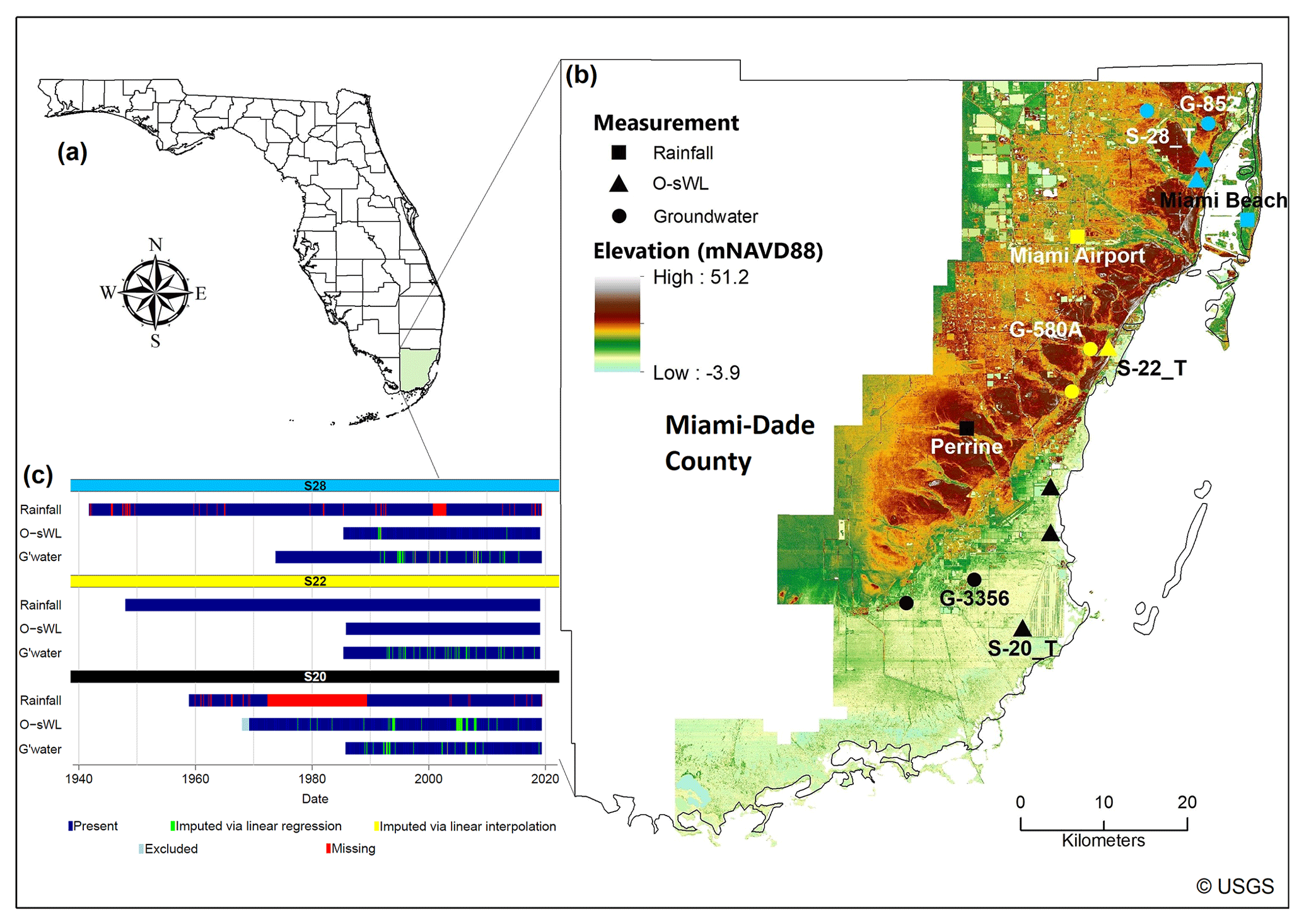
Figure 1Study site location and data completeness. (a) Miami-Dade County in the state of Florida, USA. (b) Topographical map of the eastern portion of the county showing the location of the measuring stations for the three case study sites. Principal stations are named, whilst those used for data imputation are not labelled. (c) Completeness of the records at each site's three principal stations along with the method adopted to impute specific missing values.
Rainfall data consist of daily precipitation totals obtained from the National Oceanic and Atmospheric Administration's (NOAA's) National Climatic Data Center's archive of global historical weather and climate data. The rainfall record at Miami International Airport is complete, while the records at Perrine and Miami Beach contain a substantial number of missing values, constituting 22.85 % and 4.80 % of the total time series, respectively. The highly localized nature of individual rainfall events in the region along with the spatial and temporal resolution of rainfall measurements renders the estimation of missing daily rainfall values using neighbouring gauges impractical (Pathak, 2001).
Stage gauges are attached to flood–salinity control structures operated by SFWMD. The stage time series downstream of the relevant structures (here termed O-sWL) were extracted from DBHYDRO (SFWMD's corporate environmental database) and converted to daily maxima. O-sWL refers to the still water level (i.e. the water level discounting waves/wave set-up) that comprises mean sea level, the astronomical tidal component, and non-tidal residual (Pugh, 1987). O-sWL values are given in metres above the National Geodetic Vertical Datum of 1929 (NGVD 29).
Groundwater wells (maintained by the United States Geological Survey) closest to each stage gauge and with record lengths similar to the O-sWL time series were identified and daily maximum water level records extracted from DBHYDRO. An analysis of the distribution of the missing O-sWL and groundwater observations indicated the presence of long gaps in some of the records, prohibiting linear interpolation of the record to infill missing values. However, both the O-sWL and groundwater records showed a high degree of linear correlation with corresponding records at nearby sites. Missing values were therefore imputed through a linear regression of the observations at the location of interest on those at nearby sites (Fig. S1 in the Supplement), starting with the closest site to the location of interest. Any remaining non-consecutive missing values were imputed through linear interpolation (see Figs. S2–S6).
A fundamental assumption of the standard extreme-value theory statistical models is that the analysed datasets consist of independent and identically distributed (IID) random variables. The models thus require stationarity; i.e. the statistical parameters such as mean and variance should remain constant over time and be free of “trends, shifts, or periodicity” (Salas, 1993). It is standard practice to transform the data to achieve stationarity through detrending (e.g. Wyncoll et al., 2016). The long-term mean sea level signal is superimposed onto inter-annual to multi-decadal sea level variability caused by tidal modulations associated with the nodal (18.61 year) and perigean (8.5 year) cycles, as well as other oceanic–atmospheric processes (e.g. Valle-Levinson et al., 2017). Here, a moving window approach is applied to the O-sWL series to remove long-term sea level rise and seasonality effects (Arns et al., 2013). In the procedure, the estimate of the trend is subtracted from the original time series value yielding a residual, which is then added to the mean sea level derived from the last 5 years of data to represent the most recent mean sea level conditions. The groundwater level was detrended in an identical manner. The detrended series are shown alongside the imputed observational records in Figs. S7 to S12.
Nonstationarity in the dependence between rainfall and O-sWL can occur as a consequence of a range of anthropogenically and climatically induced stressors. In this study, the dependence is assumed to be stationary, i.e. that the copula parameters remain unchanged over time. The overlapping records at the three sites are of insufficient length to robustly test the stationarity assumption. However, Wahl et al. (2015) did not detect any significant change in Kendall's τ between rainfall and surge at either Key West or Mayport, the two closest sites to Miami-Dade County, indicating stationarity to be a reasonable assumption. Nevertheless, due to regional and local effects, such as multi-decadal variation in the storm surge climate, the possibility of statistically significant trends in the dependence cannot be ruled out at the case study sites.
Section 3.1 introduces the measures for assessing the strength of the dependence between the drivers and identifying the type of dependence in their joint tail regions. Section 3.2 describes methods employed for the bivariate analysis of rainfall and O-sWL, before the choice of hazard scenario is scrutinized. Finally, Sect. 3.3 provides a description and justification for the statistical models adopted for the trivariate analysis including groundwater level.
3.1 Dependence analysis
Kendall's rank correlation coefficient τ provides a measure of the degree of the association between the variables. As opposed to linear correlation, rank correlation is able to capture any non-linear relationships between a pair of variables, whilst τ possesses several desirable properties over other rank correlation measures (Li et al., 2012). The value for each pair of variables will also be used here to determine whether there is statistically significant correlation between them, i.e. if the null hypothesis can be rejected.
Extremal dependence falls into one of two classes: asymptotic dependence or asymptotic independence (Ledford and Tawn, 1997). If (X,Y) are a pair of variables with distribution functions (Fx,Fy) transformed to common uniform (0,1) distributions, i.e. (, an intuitive measure of the extremal dependence of (X,Y) is χ (Buishand, 1984; Coles et al., 1999):
where P(A|B) is the conditional probability of A given B. For independent variables χ=0, for asymptotically dependent variables χ increases with dependence strength, and χ=1 signals perfect dependence. To obtain χ it is more convenient to consider
an asymptotically equivalent function; i.e. , for . Coles et al. (1999) introduced a second measure to quantify the magnitude of the dependence between a pair of asymptotically independent variables:
where , for and . In the case of full dependence , whilst for the class of asymptotically independent variables increases with dependence strength. Empirical estimates of χ(u) and are possible by approximating the probabilities in Eqs. (2) and (3) with the equivalent proportions observed in the data.
Svensson and Jones (2002) proposed a bootstrap procedure to test for asymptotic dependence. The two records are independently sampled with replacement using a sample size the same length as the original concurrent record. The samples are subsequently paired to create a dataset identical in size to the original but with the dependence removed. The process is repeated to create a large number N of datasets. For each dataset χ is calculated and denoted by , . If less than 5 % of values are greater than the estimate of χ associated with the observed data, then there is strong evidence against the null hypothesis . Zheng et al. (2013) used the procedures described here to assess the asymptotic behaviour of rainfall and storm surge along the Australian coastline, detecting the presence of both dependence classes.
3.2 Bivariate analysis
Here, a two-sided sampling approach similar to that in Wahl et al. (2015), which involves deriving two conditional samples where each variable is conditioned on in turn, is implemented to identify bivariate extreme events. Due to the relatively short length of the overlapping records and wastefulness of the block maxima approach, the threshold exceedance method is first used to identify univariate extremes. In practice, the method of Smith and Weissman (1994) is applied to the rainfall time series to identify cluster maxima which are paired with simultaneous O-sWL values and vice versa to create two two-dimensional time series. For more details on the choice of thresholds see Sect. 4.2.
A copula is a multivariate probability distribution with uniform marginal distributions. If X1, …, Xd are a set of d continuous random variables with joint distribution function (x1, … xd), then according to Sklar's theorem (Sklar, 1959) there exists a unique copula C on [0,1]d such that
where is the marginal distribution of Xi, i=1, … d. Hence, any multivariate joint distribution can be decomposed into the set of univariate marginal distributions and a copula. The latter contains all the information about the dependence structure of the joint distribution.
For a range of thresholds, the best fitting of 40 competing copulas plus the independence copula is determined via the Akaike information criterion (AIC), using the VineCopula R package (Schepsmeier et al., 2018). For the conditioned variable, cluster maxima above a sufficiently high threshold are fitted to a generalized Pareto distribution (GPD). The marginal non-conditioned variables are modelled by parametric distributions. Two unbounded continuous distributions are fitted to O-sWL in the sample where rainfall is conditioned to exceed a predetermined threshold. A range of continuous distributions supported on [0,∞) are fitted to rainfall in the sample where O-sWL is conditioned to exceed a predetermined threshold. In each case, several parametric tests and diagnostic plots are subsequently utilized to determine the best-fitting marginal distribution (see Supplement for more details).
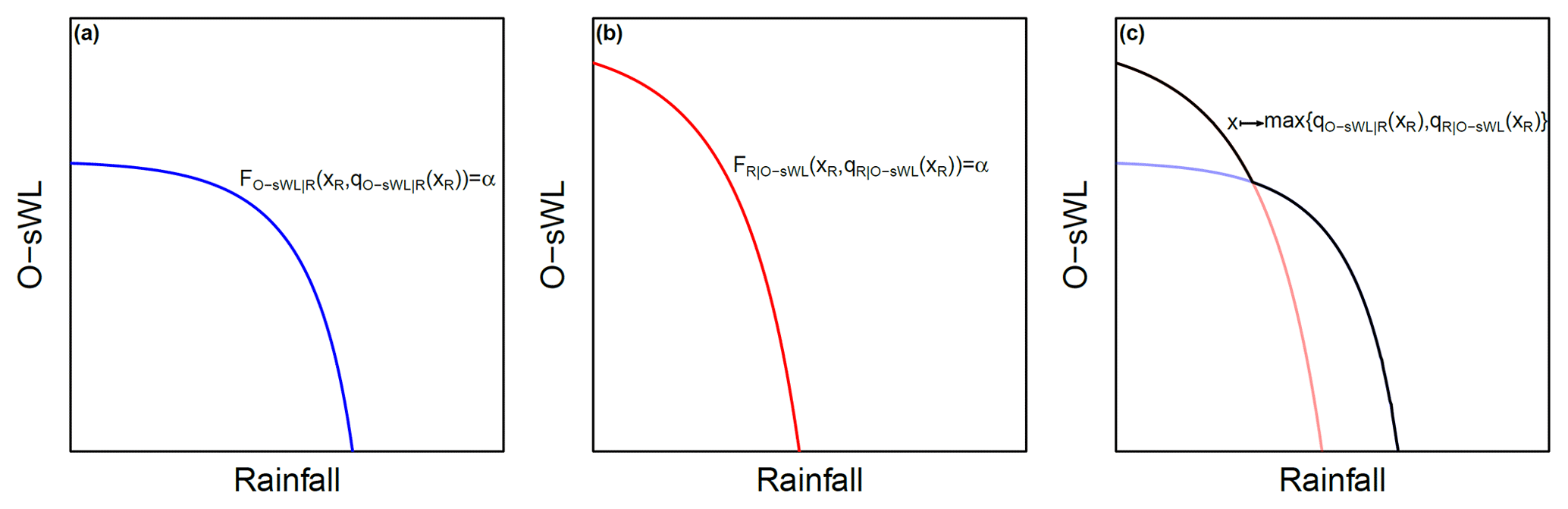
Figure 2Schematic illustrating the approach by Bender et al. (2016) for combining two isolines of level α. The (quantile-)isolines of the joint distribution from the sample conditioning on (a) rainfall and (b) O-sWL, respectively. (c) A single (quantile-)isoline is given by the envelope created by overlapping the isolines in (a) and (b).
As opposed to the univariate case where the region containing dangerous events is uniquely defined, in the bivariate and higher-dimensional settings hazard scenarios are required to specify this region. For a d-dimensional probability distribution function and , Salvadori et al. (2011) define the critical layer of level α as the following set:
The critical layer is an iso-hyper-surface of dimension d−1. Thus, it corresponds to a (iso)line (also referred to as a contour line) in the bivariate case and to a (iso)surface in the trivariate case. Each critical layer partitions Rd into three non-overlapping exhaustive regions: a super critical layer comprising the events considered dangerous, the critical layer itself, and a subcritical layer containing safe events.
There are several definitions of hazard scenarios, including OR, AND, Kendall (Salvadori et al., 2004), and survival Kendall (Salvadori et al., 2013), each offering different perceived strengths and limitations (e.g. bounded vs. unbounded subcritical layer, mathematical vs. physical valid interpretation) (e.g. Salvadori et al., 2011; Gräler et al., 2016). Due to the absence of any physical interpretation, Salvadori et al. (2016) suggest the procedures à la Kendall be reserved for preliminary assessments to gauge the expected probabilities of multivariate occurrences. The OR scenario has been extensively applied in the context of compound flooding at river confluences (e.g. Wang et al., 2009; Bender et al., 2016). Recently, Moftakhari et al. (2019) proposed incorporating the AND scenario to estimate the joint return period of river discharge and ocean levels in the FEMA (2015) procedure for assessing compound flood hazard in tidal channels and estuaries. In line with this recommendation (and many other previous applications where ocean levels and pluvial/fluvial flood drivers were analysed) the AND hazard scenario is adopted in this study.
A methodology for deriving design events when adopting a conditional sampling method with two joint probability distribution functions, as proposed in this paper, is put forward and implemented in Bender et al. (2016). The approach exploits the strict monotonicity of the joint distribution functions, by defining the (quantile-)isoline functions, for level α implicitly as and , where FO-sWL|R and FR|O-sWL are the joint distributions of the conditional samples, xR is rainfall, and qO-sWL|R(xR) and qR|O-sWL(xR) are implicit functions of rainfall. The possible design events comprise the outer envelope created by overlapping the two isolines, i.e. (see Fig. 2 for a hypothetical example illustrating the approach).
The choice of hazard scenario should reflect the type of dangerous event, e.g. a mechanism of failure, but is often an arbitrary and subjective choice (Serenaldi, 2015; Gouldby et al., 2017). Volpi and Fiori (2014) noted the typical disparity in the return period of structural failure compared with that of the loading variables and consequently proposed the so-called structure-based return period. The structure-based return period is derived by propagating the joint distribution of the basic variables through a structure or response function, describing the physical dynamics of a system. Hence, the return period of a response variable is calculated directly, typically empirically from a (large) sample of the basic variables after fitting a multivariate statistical model (Gouldby et al., 2017). The approach thus negates the need for a practitioner to define a hazard scenario (Salvadori et al., 2016). Serenaldi (2015) argues the concept of the return period in univariate frequency analysis is prone to misconceptions, only exacerbated in the multidimensional domain, and that the risk of failure offers a more transparent and suitable measure of risk. A full risk analysis is beyond the scope of this study but recommended as future work.
3.3 Trivariate analysis
This section provides a description of three types of multivariate statistical models – standard higher-dimensional copulas (Sect. 3.3.1), pair-copula constructions (Sect. 3.3.2), and the HT04 model (Sect. 3.3.3) – applied here to capture the dependence between extreme rainfall, O-sWL, and groundwater levels.
3.3.1 Standard higher-dimensional copulas
Copulas were first introduced to the field of hydrology in De Michele and Salvadori (2003), where an Archimedean copula was used to describe the dependence between storm duration and average rainfall intensity. The Archimedean copula family comprises a rich array of radially asymmetric and symmetric copulas covering a diverse range of upper and lower tail dependence. The strengths of all pairwise dependencies are captured by a single parameter; thus standard Archimedean copulas are symmetric for any permutation of indexes (exchangeability). The exchangeability of Archimedean copulas is often considered strongly restrictive in higher-dimensional applications, as it implies all pairwise dependencies are identical (Di Bernardino and Rullière, 2016). Elliptical copulas, as the name suggests, are simply copulas of elliptical distributions and consequently possess many of the useful traceable properties of these multivariate distributions (Fang et al., 1990). Elliptical copulas are radially symmetric with a correlation matrix of parameters describing the strength of the pairwise dependencies. Consequently, they are non-exchangeable, only assuming the type of dependence within each tail is identical. The trivariate Gaussian copula CGauss is given by
where ΦR is the joint cumulative distribution function (CDF) of the standard trivariate normal distribution with correlation matrix R, and Φ−1 is the inverse CDF of the univariate standard normal distribution. The Student t copula also possesses a degrees of freedom parameter υ specifying the additional probability density assigned to the joint tails compared with the Gaussian copula ceteris paribus. The Student t copula approaches the Gaussian copula as υ→∞. In contrast with the Student t copula, which possesses tail dependence, the Gaussian copula assumes asymptotic independence; i.e. the Gaussian copula has zero tail dependence χ=0.
Whilst bivariate applications are extensive in hydrology, trivariate applications of standard copulas are scarce. From analysing the dependence between drought duration, intensity, and severity in New South Wales (Australia), Wong et al. (2008) found the Gumbel copula outperformed the Gaussian copula. In a similar application in the Weihe River basin (China), Ma et al. (2013) reported that the trivariate Gaussian copula gave a better fit than the Student t copula, with both outperforming six Archimedean copulas, half of which possessed (radial) asymmetry. In other environmental applications, the Student t copula has been shown to offer a superior fit to the Gaussian copula in the presence of tail dependence (e.g. Jane et al., 2016; Wahl et al., 2016). In this study two elliptical copulas and three Archimedean copulas (Gumbel, Clayton, and Frank) are considered. The three Archimedean copulas comprise a range of tail-dependence regimes, i.e. upper, lower, and no tail dependence, and are consequently commonly applied together to assess the type of dependence between a set of variables (e.g. Daneshkhah et al., 2016).
3.3.2 Pair-copula constructions
Approaches to increase the flexibility of standard higher-dimensional copulas include techniques to remove the exchangeability property of Archimedean copulas (e.g. Di Bernardino and Rullière, 2016) as well as the development of (meta-elliptical) copulas for various meta-elliptical distributions (Fang et al., 2002). Pair-copula construction (PCC) provides greater flexibility and a more intuitive way of extending bivariate copulas to higher dimensions than these approaches (Aas et al., 2009).
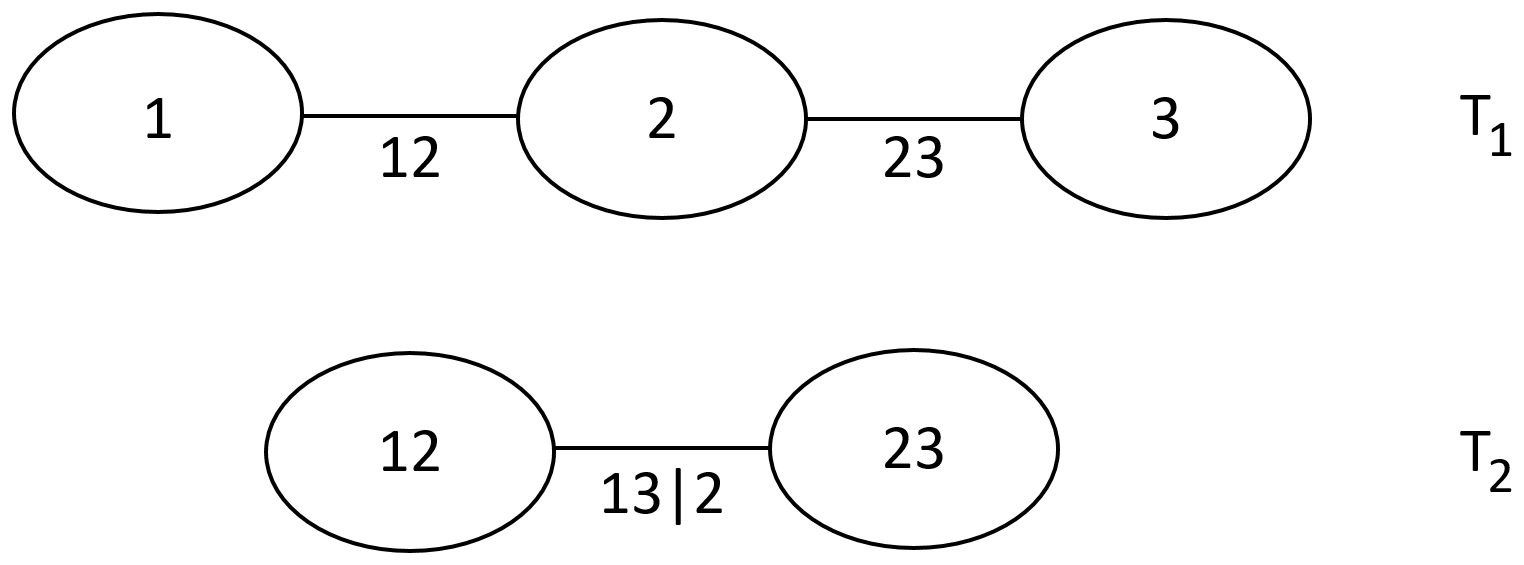
PCC, originally proposed by Joe (1996), decomposes a d-dimensional probability distribution into the product of a cascade of bivariate copulas and the marginal densities of each variable. PCC permits the free specification of copulas; the first d−1 copula densities are dependence structures of unconditional bivariate distributions, while the remaining are of conditional bivariate distributions. As d increases, the number of mathematically equally valid decompositions soon becomes large. To ensure consistent definitions of each distribution in a PCC, Bedford and Cooke (2001, 2002) introduced the regular vine, a graphical model for specifying the conditional dependencies in a decomposition. In the d-dimensional case a vine consists of a set of d−1 nested trees. The edges of tree Tj become the nodes of tree Tj+1, , where nodes represent the variables, and the labels of each edge denote the subscript of a pair-copula construction. A regular vine is a vine in which two edges are joined in tree Ti+1 only if they share a common node in tree Tj.
The class of regular vines is considered relatively broad and encompasses a range of possible pair-copula decompositions. The canonical (or C) vine and D vine are special cases of regular vines, defining specific ways of decomposing a multivariate probability density. Each of the three possible decompositions of a three-dimensional copula density are simultaneously both a C and a D vine (see Fig. 3 for one example).
Gräler et al. (2013) applied a bivariate copula to annual maximum peak discharge and its volume, as well as a trivariate vine copula, by also including duration, to investigate the effect of different modelling choices on design events. They found evidence of design quantiles shrinking as the number of variables considered grows (bivariate vs. trivariate), referred to as the dimensionality paradox (Salvadori and De Michele, 2013). They concluded that practitioners should strive for a balance between the number of variables considered and (numerical) complexity of the copula. In a similar study, Daneshkhah et al. (2016) showed a vine copula outperformed five tested standard higher-dimensional multivariate copulas.
An alternative pair-copula decomposition of a higher-dimensional joint probability distribution is the nested Archimedean construction (NAC) (e.g. Embrechts et al., 2003). In NAC, only d−1 copulas are user specified, whilst the remaining copula and parameters are defined implicitly through the construction. In addition, the bivariate copulas are required to be Archimedean copulas, and there are strong restrictions on the parameters. After the application of PCC and NAC to two four-dimensional financial and environmental datasets, Aas and Berg (2009) concluded that PCC is superior in terms of both goodness of fit and computational efficiency.
3.3.3 Heffernan and Tawn (HT04) approach
The HT04 approach models the conditional distribution of the remaining variables given a specified variable exceeds a suitably high threshold. By repeating the procedure for each variable in turn, the model captures the dependence structure between a set of variables when at least one takes on an extreme value. The HT04 approach thus requires no assumptions regarding the nature of the dependence in the joint tail regions between a set of variables.
As opposed to the standard copula methodology, the HT04 model is generally implemented using Gumbel marginal distributions given by , where is an estimate of the cumulative distribution function of Xi. Alternative scales can be invoked to transform the data to common marginals. For instance, Keef et al. (2013) describe the advantages of using Laplace scales, particularly if any variables exhibit a negative association. To remain consistent with HT04 and most other applications of the approach, Gumbel scales are adopted in this work. If Y−i is the vector of all the (transformed) variables excluding Yi, the HT04 model is typically implemented via the following multivariate non-linear regression model:
where υ is a suitably high threshold on Yi, a and b are vectors of parameters, and Z is a vector of residuals. The parameters a and b are estimated using maximum likelihood under the temporary assumption that Z is normally distributed with unknown mean and variance. Recently, Towe et al. (2019) removed the temporary Gaussian assumption on the joint residual distribution by instead modelling the distribution semi-parametrically using a Gaussian copula and kernel-density-estimated marginals. This alteration permits new combinations of Z to arise, thus enabling non-deterministic extrapolation of past events; in the context of the present study this is to be considered in future work.
An outline of the steps involved in the well-established Monte Carlo procedure for generating a realization Y (on the transformed scale) from the fitted model is given below (e.g,. Keef et al., 2009a; Gouldby et al., 2014):
-
sample Yi, conditional on Yi>υ;
-
independently sample a joint residual Z;
-
calculate Y−i from Eq. (9) using relevant regression parameters, Yi, Z;
-
reject sample Y, unless Yi is a maximum.
Given the desired sample dimension, the sequence of steps is repeated until the expected number of events where variable Yi is a maximum, conditioned to exceed the threshold, is consistent with the empirical distribution. The procedure is repeated, conditioning on each variable in turn to ensure the appropriate proportion of events are simulated. The sample can then be transformed to original scales using the marginal distributions and the inverse probability integral transform.
The extremes observed during such temporal dependent and spatially varying events may not occur concurrently. Keef et al. (2009a) addressed this limitation by fitting the HT04 model to the distribution of the variable at location j at a lag of τ in relation to an extreme value observed at location i; i.e. the model is fitted to for , for a range of τ and each i≠j. Subsequently, Keef et al. (2009b) applied the method to investigate the spatial dependence of rainfall and river flow in Great Britain and found that both types of extreme events become increasingly localized with increasing return period. Similarly, multi-site, single-variable applications are common in the literature (e.g. Lamb et al., 2010; Diederen et al., 2019). The model has also been applied to capture the dependence in the variables contributing to extreme sea states at a single location (e.g. Gouldby et al., 2014) and at multiple sites (Wyncoll et al., 2016).
In this section, the results of the correlation analysis (Sect. 4.1), bivariate analysis (Sect. 4.2), and trivariate analysis (Sect. 4.3) are discussed in turn. In Sect. 4.2 and 4.3 results pertain to site S22; analogous results for the other two sites are provided in the Supplement.
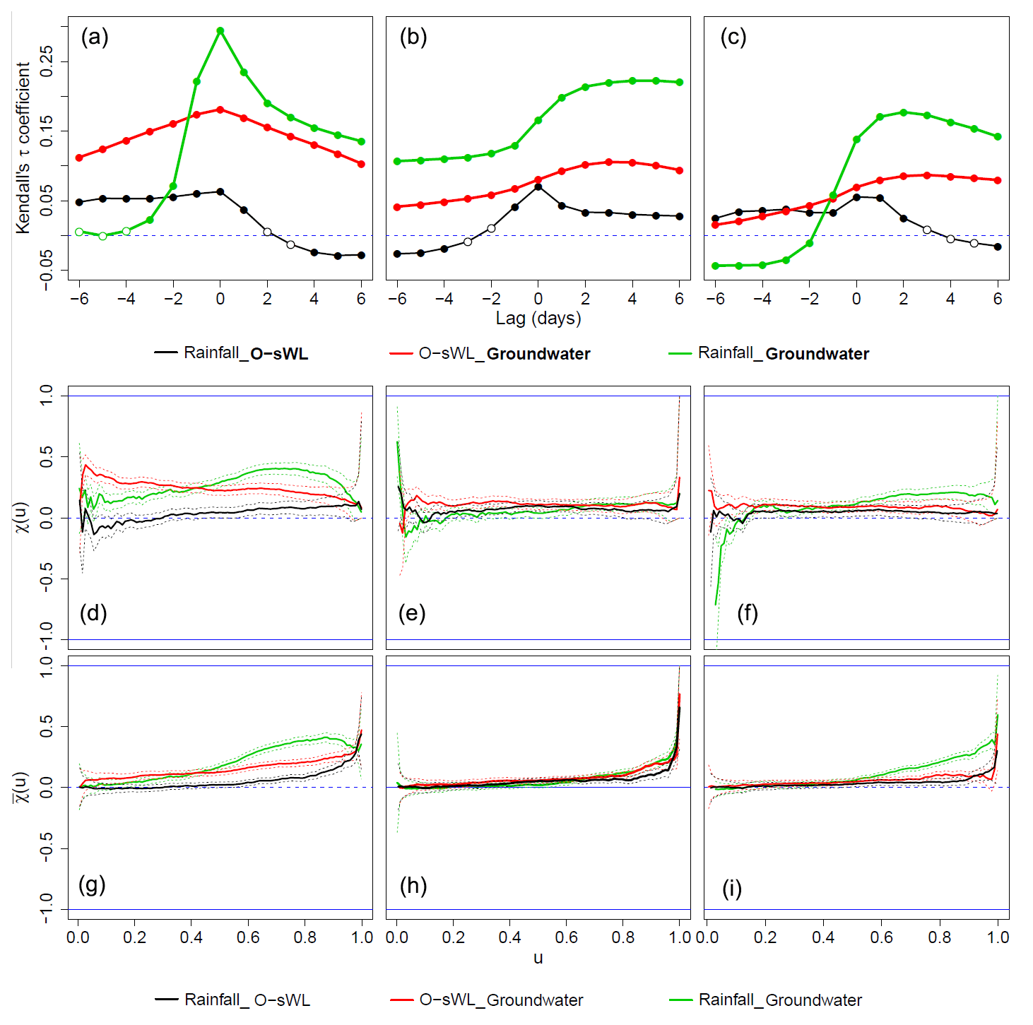
Figure 4Assessment of correlation between the flooding drivers at site S20 (a, d, g), S22 (b, e, h) and S28 (c, f, i). (a–c) Measure of the pairwise association τ between the drivers over various lags. Filled dots indicate the presence of statistically significant correlations (p value < 0.05). The lag is applied to the quantity shown in bold. (d–i) Estimates of χ(u) and along with the associated 95 % confidence intervals.
4.1 Dependence analysis
Rainfall, O-sWL, and groundwater level exhibit small (τ<0.3) but generally statistically significant correlations over a range of time lags (Fig. 4a–c). The strength of the correlation of rainfall and O-sWL with groundwater level decreases with distance north across study sites. In addition, the peaks in the correlations are situated at zero lag at site S20 but at lags in the groundwater level of between 2 and 4 d at sites S22 and S28, respectively. The peaks in these correlations also become increasingly shallow with distance north, indicating that the water table is more responsive at S20 than at the other sites. This is likely a consequence of the lower elevation at S20, resulting in the water table typically laying closest to the ground surface. Rainfall and O-sWL are the least correlated of the variable pairs, exhibiting little variation in correlation strength or variation with lag between the sites. To ensure that temporally coherent combinations of the drivers are simulated, no lags are considered in either the bivariate or trivariate analysis. For instance, applying a lag to the groundwater level will account for its maximum correlation with O-sWL and rainfall at sites S22 and S28. However, by the time the elevated groundwater level arises, the high O-sWL may have dissipated and rainfall potentially ceased; thus it is possible the drivers do not produce any compounding effects.
The empirical estimates of χ(u) and as u→1 (Fig. 4d–i) provide an informal assessment of the asymptotic behaviour of the joint distribution of the drivers. The informal analysis failed to provide conclusive evidence of asymptotic dependence or asymptotic independence, an issue also highlighted in Coles et al. (1999). For instance, at site S20 the best estimate of χ for each pair of drivers is positive once u>0.4, indicating asymptotic dependence. However, the confidence intervals for χ always include zero and , contradicting the conclusion of asymptotic dependence. On the other hand, all pairs of drivers at all sites returned statistically significant results in the hypothesis test proposed in Svensson and Jones (2002), providing strong evidence against the null hypothesis of asymptotic independence.

Figure 5Comparison of the design events (diamonds) obtained using the two-sided conditional sampling approach and the approach used in the original design (triangles) for return periods of (a) 10, (b) 20, (c) 50, and (d) 100 years. Quantile-isolines are superimposed onto plots of the observations, with blue circles (red crosses) denoting observations exceeding the rainfall (O-sWL) threshold and those exceeding neither threshold plotted in grey. Coloured contours signify the relative likelihood of events along an isoline, where the point with the highest density is selected as the most-likely design event. Insets in (a) and (b) magnify the isoline about the associated most-likely design event.
4.2 Bivariate analysis
To capture the dependence between rainfall and O-sWL, the approach outlined in Sect. 3.2 was applied for a range of thresholds. The choice of copula family is relatively insensitive to the selected threshold (see Figs. S13 to S15). The threshold is selected as a trade-off between the bias and variance in the copula parameter estimates. For each of the conditioned samples a threshold of the 0.98 quantile of the conditioning variable was deemed appropriate at each of the sites. Attention from hereon in focuses on site S22 (detailed results for the other sites are included in the Supplement), where the 0.98 quantile threshold gives an average of 6.3 and 5.2 events per year when conditioning on O-sWL and rainfall, respectively. The conditioning variable was fitted to a GPD while relevant non-extreme parametric distributions were fitted to the non-conditioning variable. The Birnbaum–Saunders(logistic) distribution was selected to model the rainfall(O-sWL) data in the sample where O-sWL(rainfall) is conditioned to exceed its 0.98 quantile, as it was consistently among the best fitting of the candidate distributions at the three sites (see Figs. S16 to S18).
The quantile isolines for several return periods are shown alongside the observations in Fig. 5. The coloured contours on the isolines represent the relative likelihood of events. The most-likely strategy is used as a simple way to derive possible design events associated with a given return period T (Salvadori et al., 2011, 2013). Practically, the design event is given by the point of maximum relative probability density on the isoline associated with return period T. In this work, the relative probabilities are estimated non-parametrically via a kernel density estimate (KDE), using the ks R package (Duong, 2007). Initially KDE was applied to the observations; however, particularly for larger return periods the design event proved highly sensitive to a small number of observations. Hence, design events were determined by applying KDE to a large sample (N=10 000) from the two fitted copulas, with sample proportions consistent with the empirical distributions, and transformed back to original scales. The probability density given by the KDE at points along the isoline are extracted and the probabilities scaled to lie within [0,1], hence yielding relative probabilities.
Figure 5 illustrates two types of design events, indicating that the system experiences a change in behaviour between 20- and 50-year return periods. To further investigate the return period at which the change in design event type occurs, design events were calculated for return periods from 1 to 100 years at a yearly interval. The processes of simulating samples from the fitted copulas, estimating the relative likelihood along the isolines and extracting the most-likely event, was then repeated to give 100 design events associated with the 1- to 100-year return periods. The results showed that the change occurs for return periods between approximately 20 and 40 years. For small return periods (≤ 20 years), design event rainfall remained < 1 mm; thus they may be considered “surge-only” events. Consequently, the original design events are only marginally conservative in terms of O-sWL yet highly conservative with respect to rainfall. For return periods, greater than say 40 years, design events resemble compound events. As the return period increases, rainfall values given by the bivariate approach increasingly resemble the corresponding univariate return period rainfall (i.e. the most-likely event moves to the right along the x axis). Conversely, the O-sWL of the design event given by the new and original design approaches diverge as return periods increase (i.e. the most-likely design event moves down along the y axis). For instance, the O-sWL in the design event given by the bivariate approach in Fig. 5 is 0.47 m less than that in the original design approach for a 50-year return period, and the difference increases to 0.61 m for the 100-year return period event. For return periods between 20 and 40 years both surge-only and compound events arise, depending on the sample simulated from the fitted copulas.
Most-likely design events that are surge only (for smaller bivariate return periods) will potentially produce very different water levels at a structure (response variable) compared to compound events (for higher bivariate return periods), ultimately resulting in substantially different design conditions. For several flood defences in England, Gouldby et al. (2017) illustrated the sensitivity of the return period of a response variable – overtopping discharge – to the choice of return period definition. To account for the variability in design event selection, approaches have been developed to replace single design events with ensembles of possible design realizations (Gräler et al., 2013). Testing an ensemble of design events or adopting a structurally based return period, where extremes are defined in terms of response variables directly, will produce a more robust analysis. Implementation of these approaches would be particularly beneficial at sites S20 and S28, where, although all design events can be classified as surge only, probability density is non-zero along other parts of the isolines (see Figs. S19 and S20). In many cases implementing these approaches requires running complex and computationally expensive process-based models and is therefore beyond the scope of our analysis.
The conservative nature of the original design approach is further explored by assessing how long it will take under a given SLR for the 100-year design events selected with the two different methods (i.e. full dependence assumption vs. bivariate dependence modelling) to intersect. In other words, the amount of SLR and how long it will take under different emission scenarios, for the diamonds (i.e. bivariate design events) in Fig. 5 to move vertically and close the gap to the triangles (i.e. design events under full dependence assumption, used in the original design), is assessed. The low, intermediate, and high scenarios from Sweet et al. (2017) are considered (see Fig. 6, top).
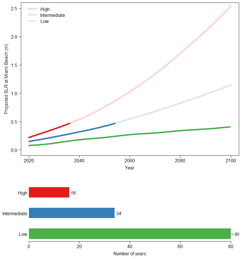
Figure 6The top shows regional SLR projections for Miami Beach given in Sweet et al. (2017). The bottom shows the number of years before the O-sWL in the 50-year design event derived using the bivariate approach reaches the corresponding value obtained using the original design approach according to the three SLR scenarios.
The results are highly sensitive to the SLR scenario considered. For instance, the time before the O-sWL in the 50-year bivariate approach reaches that of the corresponding event derived using original design approach ranges from 16 years to greater than 80 years (Fig. 6, bottom). The times before the O-sWL in the design events given by the original design and bivariate approaches with return periods from 1 to 100 years become equal according to the three scenarios shown in Fig. 7. The change in the characteristic of the design events (i.e. the shift from O-sWL dominated to compound driven) between return periods of around 20 to 40 years is apparent. For events with return periods > 40 years, the time required for the O-sWL of the design events given by the two approaches to coincide increases linearly with the return period. According to the low-SLR scenario the bivariate copula analysis combined with the most-likely design point suggests the currently employed assumption of full dependence between drivers is highly conservative, inadvertently incorporating safety factors sufficient to account for SLR beyond the year 2100. Conversely, under the high-SLR scenario the bivariate design assessment implies that the current approach is less conservative, with safety factors being exhausted within approximately 30 years for all return periods considered here (up to 100 years).
The disparity of the rainfall totals composing the design events given by the bivariate and original design approaches is greatest for low return periods (< 20 years), as demonstrated in Fig. 5. It is possible that the rainfall totals will equate in the future due to changes in rainfall patterns. However, rainfall projections were not examined here due to their large uncertainties and the lack of guidance regarding their coupling with SLR scenarios. Moreover, low-return-period events (< 20 years) are not typically used in structural design.
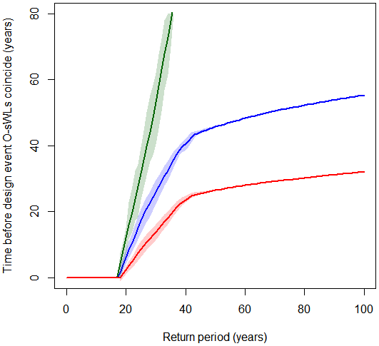
Figure 7Time before the O-sWL in the bivariate design event derived from the two-sided sampling approach reaches the corresponding value obtained from the original design approach (i.e. full dependence assumption) under the low (green), intermediate (blue), and high (red) SLR scenarios given in Sweet et al. (2017). Shaded regions denote 95 % (basic) bootstrap confidence intervals.
4.3 Trivariate analysis
In this section, the bivariate analysis is extended by also incorporating groundwater level into the analysis. First, the marginal extremes are analysed separately for each flooding driver. The method of Smith and Weissman (1994) was applied to each time series to identify cluster maxima. For each variable, cluster maxima and excesses above a sufficiently high threshold were fitted to a GPD. The GPD was combined with the empirical distribution below the threshold. The threshold choice was guided by appropriate criteria, predominantly mean residual life plots (Coles, 2001). Diagnostic goodness of fit demonstrated the adequacy of the fit plots of the GPD for the rainfall and groundwater level series, whilst the fit to the O-sWL series was less robust (see Figs. S21 to S29). The study area is exposed to several flood-generating mechanisms including storms associated with tropical cyclones, mesoscale convective systems, and extratropical systems. Hence, a single distribution is fitted to events that are likely coming from several different populations. The fit of the GPD was particularly poor for the three largest O-sWL events. The five highest recorded O-sWL values are associated with tropical cyclones, consistent with an analysis by Villarini and Smith (2010). Nevertheless, observational records of the length available for this study contain relatively few tropical cyclone events. Consequently, risk assessments in areas exposed to tropical cyclone storm surges commonly utilize synthetic records of such events, generated based on historical observations (e.g. Nott, 2016). To generate synthetic records, wind and pressure fields simulated from statistical models of tropical cyclone behaviours are used to drive hydrodynamic storm surge models (Haigh et al., 2014). Replacing the observational record with a longer synthetic record could thus be an avenue to improve the marginal fit of the O-sWL distribution and ultimately the robustness of the proposed approach. This is beyond the scope of the present study, where the focus is on developing appropriate frameworks for capturing and modelling dependence between the different flood drivers.
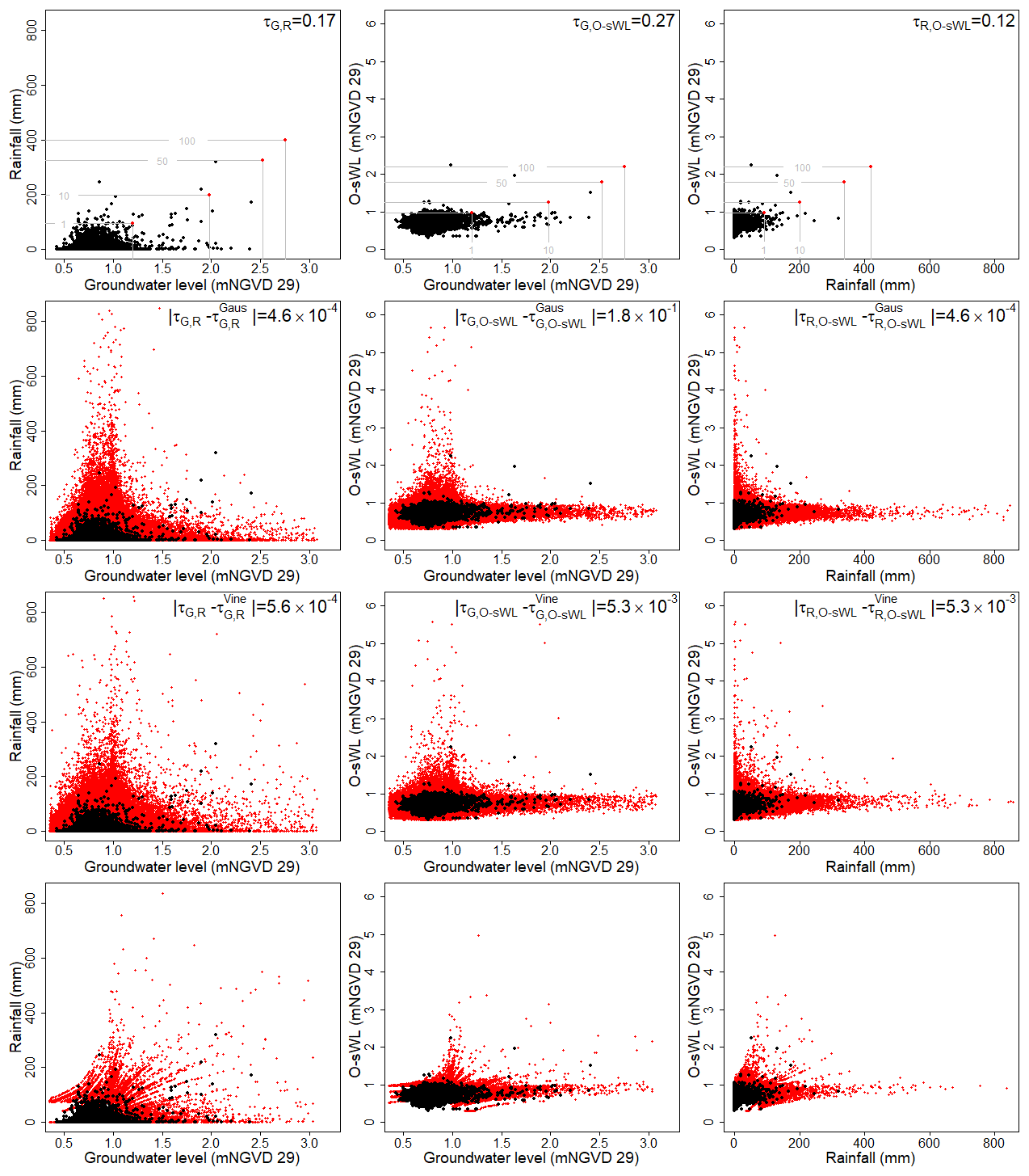
Figure 8(First row) Observed events at site S22 (black dots) superimposed with the T year return levels (grey lines) obtained from the marginal distributions and corresponding design events under the full dependence assumption (red dots). Kendall's τ coefficients are also displayed. Observed events (black dots) alongside 10 000-year synthetic event records (red dots) generated using the (second row) Gaussian copula, (third row) Vine copula, and (fourth row) HT04 models.
The multivariate model fitting also requires sets of independent events. Gouldby et al. (2014) used a notional flooding level, a function of the primary variables of interest, to de-cluster the offshore loading time series data before fitting the HT04 model. In other applications of the HT04 approach, marginal de-clustered excesses of the conditioning variable are paired with concurrent values of the remaining variables. The nonlinear regression model (Eq. 7) is then fitted to the set of events and the process is repeated conditioning on each variable in turn. In the absence of a suitable response function that can be evaluated without employing hydraulic–hydrologic models, this is also the approach adopted here in the application of the HT04 model. Standard higher-dimensional copulas and vine copula models are often applied conditioning on a single variable to derive a set of independent events. However, only conditioning on a single variable may result in the removal of the most extreme values of the other variables. Therefore, in this work the models are applied to the entire dataset, as implemented before for higher-dimensional copulas in Wong et al. (2008) and for vine copulas in Bevacqua et al. (2017), among others.
At all three sites, the Gaussian and Student t copula provided a similar fit in terms of AIC, which is far superior to that of the Archimedean copulas. The Gumbel copula was the only one of the considered Archimedean copulas to exhibit positive upper tail dependence and resulted in the best fit among the three tested Archimedean copulas. For the three sites, scatter plots of the observations against 10 000 years worth of simulated data and Kendall's τ correlation coefficients indicate the vine copula offers a superior fit compared to the Gaussian copula (see Fig. 8 for the results at site S22 and Figs. S30 and S31 for the corresponding plots at the other two sites). The plots also show that the HT04 model appears the most adept of the three approaches at capturing the dependence, particularly between O-sWL and the other variables. Overall the sparsity of simulation data near the design events (with return periods greater than 1 year) obtained under the assumption of full dependence demonstrates the importance of accounting for the dependencies between the drivers when assessing the compound flood hazard.
The return periods conditional on a range of antecedent groundwater levels for the four bivariate (most-likely) design events, accounting for the dependence between rainfall and O-sWL (diamonds in Fig. 5), according to the three types of trivariate models are shown in Fig. 9. The trivariate return periods are calculated empirically from the samples in Fig. 8. The bivariate events with return periods of 50 and 100 years were assigned return periods of > 1000 years by the Gaussian and vine copulas for the groundwater levels considered and hence do not appear in Fig. 9. In the case of the vine copula and Gaussian copula, the 10- and 20-year bivariate design events exhibit sharp increases in return period about a narrow band of groundwater levels around 1 mNGVD 29. Given that the rainfall component of these bivariate design events is negligible (see Fig. 5a and b), the steep increases in return periods are consistent with the spike in simulations centred on this narrow band of groundwater levels seen in the two middle plots in the middle column of Fig. 8. When extending the original design approach to include groundwater level, the annual exceedance event (i.e. trivariate event comprising the rainfall, O-sWL, and groundwater level with univariate return periods of 1 year) possesses return periods of 2000, 227, and 116 years according to the Gaussian copula, vine copula, and HT04 approaches, respectively. Similar patterns emerge when considering the co-occurrence of groundwater level and either rainfall or O-sWL (see Figs. S32 and S33). Hence, differences between joint probabilities under the full dependence assumption currently used in FPLOS assessments and when accounting for actual dependencies increases further in the trivariate domain.
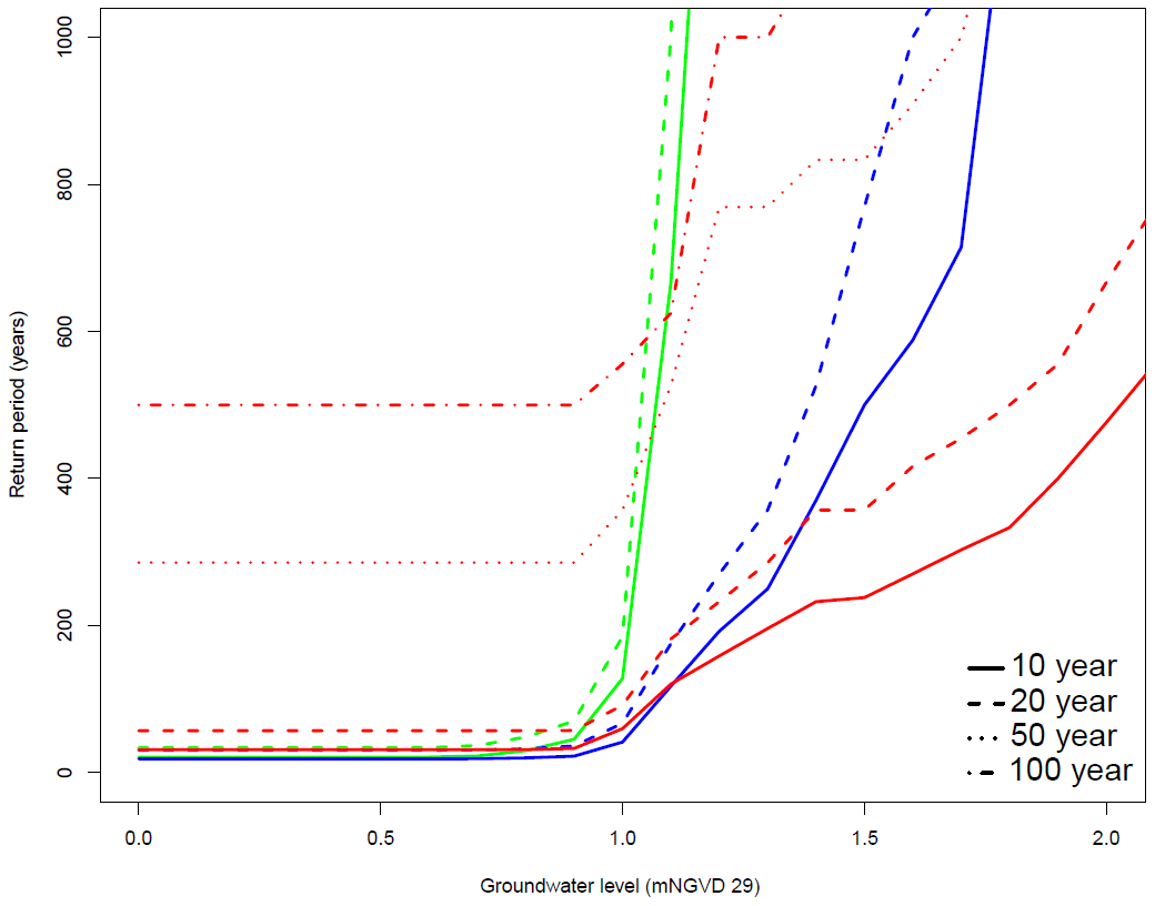
Figure 9Sensitivity of the return period of the four bivariate design events, derived using the approach described in Sect. 3.1 and displayed in Fig. 4, to the antecedent catchment condition. The trivariate return periods are calculated using the Gaussian copula (green), vine copula (blue), and HT04 (red) approach.
This paper puts forward a framework for assessing the different drivers of compound flooding in coastal areas of south Florida in Miami-Dade County. The framework was derived through a gradual transition from the original structural design approach (based on the assumption of full dependence between rainfall and O-sWL and ignoring groundwater levels) by meeting three objectives. The first objective was to determine whether there is any statistically significant correlation between extreme rainfall, O-sWL, and groundwater level in the area. At all three study sites, rainfall, O-sWL, and groundwater level exhibit small but statistically significant pairwise correlations over a range of relevant time lags. The second objective was to assess the conservative nature of the original structural design approach that assumes full dependence. This was achieved by combining a bivariate analysis of the two flooding drivers rainfall and O-sWL with regional relative SLR scenarios. In the bivariate analysis, at site S22, low-return-period (< 20 year) design events constituted surge-only events; hence the original design approach is deemed highly conservative with respect to rainfall but less so in terms of O-sWL. The approach was shown to become ever more conservative in terms of O-sWL as return periods increase. The overall magnitude of the conservative assumption was found to be highly dependent on the SLR scenario considered. For instance, any safety margin in the design according to the original approach for design events with return periods greater than 35 years is exhausted in less than 32 years under the high-SLR scenario. Conversely, for events with return periods up to 100 years, this is expected to take more than 80 years under the low-SLR scenario. At sites S20 and S28, although the bivariate design events for return periods 1 and 100 years were surge events, probability density is non-zero along other parts of the isoline. The final objective was to provide robust estimates of the joint probabilities of extreme rainfall, O-sWL, and groundwater table for implementation in future FPLOS assessments. Three types of multivariate statistical models – five standard higher-dimensional copulas, the vine copula, and the HT04 model – were applied to capture the dependence structure in the extremes of rainfall, O-sWL, and groundwater level. The vine copula and HT04 models capture the dependence better than any of the five tested standard higher-dimensional copulas.
The output of the bivariate and particularly trivariate applications can also act as boundary conditions for coupled hydrologic–hydraulic models for assessing flood risk and designing flood defence structures, among other purposes (e.g. Serafin et al., 2019). Rigorous implementation of the bivariate and trivariate methodologies, e.g. by adopting a structure-based return period approach or using an ensemble of events, will potentially facilitate more effective flood risk management in low-lying coastal catchments. A natural next step would be to explore the influence of the more robust boundary conditions on the design specifications of the water control structures at the three sites. Meanwhile, the accuracy of the GPD fit to O-sWL at the study sites (especially in the trivariate analysis; see Figs. S22, S25 and S28) could also be improved by utilizing synthetic tropical cyclone events and associated storm surges. The methodologies introduced here are readily transferable and applicable to other locations, assuming sufficiently long overlapping records of the different variables are available.
Code and data used to complete this study are available in the MultiHazard R package, which can be downloaded from GitHub at https://github.com/rjaneUCF/MultiHazard (last access: 20 August 2020) (Jane, 2020).
See Code availability section. The data used in this paper are also freely available through NOAA's National Climatic Data Center's (NCDC) archive of global historical weather and climate data at https://www.ncdc.noaa.gov/cdo-web (last access: 12 April 2019) (NOAA, 2019) (rainfall) and SFWMD's corporate environmental database DBHYDRO at https://www.sfwmd.gov/science-data/dbhydro (last access: 6 April 2019) (SFWMD, 2019) (O-sWL and groundwater level).
The supplement related to this article is available online at: https://doi.org/10.5194/nhess-20-2681-2020-supplement.
The study was conceived by JO and TW. RJ developed the methodology, undertook the analyses, and wrote the paper under the guidance of TW. LC and JO contributed by generating ideas, providing valuable insights during technical discussions, and editing the manuscript.
Thomas Wahl is on the Editorial Board of this special issue.
This article is part of the special issue “Advances in extreme value analysis and application to natural hazards”. It is a result of the Advances in Extreme Value Analysis and application to Natural Hazard (EVAN), Paris, France, 17–19 September 2019.
Robert Jane was supported by funding from the South Florida Water Management District. Thomas Wahl acknowledges financial support from the USACE Climate Preparedness and Resilience Community of Practice. This material is based in part on work supported by the National Science Foundation under grant AGS-1929382 (Thomas Wahl).
This paper was edited by Sylvie Parey and reviewed by Hamed Moftakhari and one anonymous referee.
Aas, K. and Berg, D.: Models for construction of multivariate dependence – a comparison study, Eur. J. Financ., 15, 639–659, 2009.
Aas, K., Czado, C., Frigessi, A., and Bakken, H.: Pair copula constructions of multiple dependence, Insurance: Math. Econ., 44, 182–198, 2009.
Arns, A., Wahl, T., Haigh, I. D., Jensen, J., and Pattiaratchi, C.: Estimating extreme water level probabilities: A comparison of the direct methods and recommendations for best practise, Coast. Eng., 81, 51–66, 2013.
Bedford, T. and Cooke, R. M.: Probability density decomposition for conditionally dependent random variables modeled by vines, Ann. Math. Artif. Intel., 32, 245–268, 2001.
Bedford, T. and Cooke, R. M.: Vines – a new graphical model for dependent random variables, Ann. Stat., 30, 1031–1068, 2002.
Bender, J., Wahl, T., Müller, A., and Jensen, J.: A multivariate design framework for river confluences, Hydrolog. Sci. J., 61, 3471–482, 2016.
Bengtsson, L.: Probability of combined high sea levels and large rains in Malmö, Sweden, southern Öresund, Hydrol. Process., 30, 3172– 3183, 2016.
Berghuijs, W. R., Woods, R. A., Hutton, C. J., and Sivapalan, M.: Dominant flood generating mechanisms across the United States, Geophys. Res. Lett., 43, 4382–4390, 2016.
Berghuijs, W. R., Harrigan, S., Molnar, P., Slater, L. J., and Kirchner, J. W.: The relative importance of different flood-generating mechanisms across Europe, Water Resour. Res., 55, 4582–4593, 2019.
Bevacqua, E., Maraun, D., Hobæk Haff, I., Widmann, M., and Vrac, M.: Multivariate statistical modelling of compound events via pair-copula constructions: analysis of floods in Ravenna (Italy), Hydrol. Earth Syst. Sci., 21, 2701–2723, https://doi.org/10.5194/hess-21-2701-2017, 2017.
Bevacqua, E., Maraun, D., Vousdoukas, M. I., Voukouvalas, E., Vrac, M., Mentaschi, L., and Widmann, M.: Higher probability of compound flooding from precipitation and storm surge in Europe under anthropogenic climate change, Sci. Adv., 5, eaaw5531, https://doi.org/10.1126/sciadv.aaw5531, 2019.
Bevacqua, E., Vousdoukas, M. I., Shepherd, T. G., and Vrac, M.: Brief communication: The role of using precipitation or river discharge data when assessing global coastal compound flooding, Nat. Hazards Earth Syst. Sci., 20, 1765–1782, https://doi.org/10.5194/nhess-20-1765-2020, 2020.
Bloetscher, F. H., Heimlich, B., and Meeroff, D. E.: Development of an adaptation toolbox to protect southeast Florida water supplies from climate change, Environ. Rev., 19, 397–417, 2011.
Buishand, T. A.: Bivariate extreme-value data and the station-year method, J. Hydrol., 69, 77–95, 1984.
Chen, L., Singh, V. P., Shenglian, G., Hao, Z., and Li, T.: Flood coincidence risk analysis using multivariate copula functions, J. Hydrol. Eng., 17, 742–755, 2012.
Coles, S.: An Introduction to Statistical Modelling of Extreme Values, Springer series in statistics, Springer-Verlag, London, 2001.
Coles, S. G., Heffernan, J. E., and Tawn, J. A.: Dependence measures for extreme value analyses, Extremes, 2, 339–365, 1999.
Couasnon, A., Sebastian, A., and Morales-Nápoles, O.: A Copula-Based Bayesian Network for Modeling Compound Flood Hazard from Riverine and Coastal Interactions at the Catchment Scale: An Application to the Houston Ship Channel, Texas, Water, 10, 1190, https://doi.org/10.3390/w10091190, 2018.
Couasnon, A., Eilander, D., Muis, S., Veldkamp, T. I. E., Haigh, I. D., Wahl, T., Winsemius, H. C., and Ward, P. J.: Measuring compound flood potential from river discharge and storm surge extremes at the global scale, Nat. Hazards Earth Syst. Sci., 20, 489–504, https://doi.org/10.5194/nhess-20-489-2020, 2020.
Daneshkhah, A., Remesan, R., Chatrabgoun, O., and Holman, I. P.: Probabilistic modeling of flood characterizations with parametric and minimum information pair-copula model, J. Hydrol., 540, 469–487, 2016.
De Michele, C. and Salvadori, G.: A Generalized Pareto intensity-duration model of storm rainfall exploiting 2-Copulas, J. Geophys. Res., 108, 4067, https://doi.org/10.1029/2002JD002534, 2003.
Di Bernardino, E. and Rullière, D.: On an asymmetric extension of multivariate Archimedean copulas based on quadratic form, Depend. Model., 4, 328–347, 2016.
Diederen, D., Liu, Y., Gouldby, B., Diermanse, F., and Vorogushyn, S.: Stochastic generation of spatially coherent river discharge peaks for continental event-based flood risk assessment, Nat. Hazards Earth Syst. Sci., 19, 1041–1053, https://doi.org/10.5194/nhess-19-1041-2019, 2019.
Duong, T.: ks: Kernel density estimation and kernel discriminant analysis for multivariate data in R, J. Stat. Softw., 21, 1–16, 2007.
Embrechts, P., Lindskog, F., and McNeil, A.: Modelling dependence with copulas and applications to risk management, in: Handbook of Heavy Tailed Distributions in Finance, edited by: Rachev, S. T., North-Holland, Elsevier, the Netherlands, 2003.
Fang, H.-B., Fang, K., and Kotz, S.: The meta-elliptical distributions with given marginals, J. Multivariate Anal., 82, 1–16, 2002.
Fang, K. T., Kot, S., and Ng, K. W.: Symmetric Multivariate and Related Distributions, Chapman and Hall, London, 1990.
FEMA: Guidance for flood risk analysis and mapping; combined coastal and riverine floodplain, No. Guidance Document 32, FEMA, Washington, D.C., 2015.
Flood Control Act of 1948, Pub. L. 80–858, 46 Stat. 925, United States Congress, 1948.
Florida Office of Economic and Demographic Research: Florida Demographic Estimating Conference April 2015 and the University of Florida, Bureau of Economic and Business Research, Florida Population Studies, Bulletin 178, June 2015.
Ganguli, P. and Merz, B.: Extreme Coastal Water Levels Exacerbate Fluvial Flood Hazards in Northwestern Europe, Sci. Rep.-UK, 9, 13165, https://doi.org/10.1038/s41598-019-49822-6, 2019.
Gilja, G., Ocvirk, E., and Kuspilić, N.: Joint probability analysis of flood hazard at river confluences using bivariate copulas, Gradevinar, 70, 267–275, 2018.
Gräler, B., van den Berg, M. J., Vandenberghe, S., Petroselli, A., Grimaldi, S., De Baets, B., and Verhoest, N. E. C.: Multivariate return periods in hydrology: a critical and practical review focusing on synthetic design hydrograph estimation, Hydrol. Earth Syst. Sci., 17, 1281–1296, https://doi.org/10.5194/hess-17-1281-2013, 2013.
Gräler, B., Petroselli, A., Grimaldi, S., De Baets, B., and Verhoest, N.: An update on multivariate return periods in hydrology, P. Int. Ass. Hydrol. Sci., 373, 175–178, 2016.
Gouldby, B., Méndez, F. J., Guanche, Y., Rueda, A., and Mínguez, R.: A methodology for deriving extreme nearshore sea conditions for structural design and flood risk analysis, Coast. Eng., 88, 15–26, 2014.
Gouldby, B. P., Wyncoll, D., Panzeri,M., Franklin, M., Hunt, T., Hames, D., Tozer, N. P., Hawkes, P. J., Dornbusch, U., and Pullen T. A.: Multivariate extreme value modelling of sea conditions around the coast of England, P. I. Civil Eng.-Mar. En., 170, 3–20, 2017.
Haigh, I. D., MacPherson, L. R., Mason, M. S., Wijeratne, E. M. S., Pattiaratchi, C. B., Crompton, R. P., and George, S.: Estimating present day extreme water level exceedance probabilities around the coastline of Australia: tropical cyclone-induced storm surges, Clim. Dynam., 42, 139–157, 2014.
Hallegatte, S., Green, C., Nicholls, R. J., and Corfee-Morlot, J.: Future flood losses in major coastal cities, Nat. Clim. Change, 3, 802–806, 2013.
Hawkes, P. J.: Joint Probability Analysis for Estimation of Extremes, J. Hydraul. Res., 46, 246–256, 2008.
Hawkes, P. J., Gouldby, B. P., Tawn, J. A., and Owen, M. W.: The joint probability of waves and water levels in coastal engineering design, J. Hydraul. Res., 40, 241–251, 2002.
Heffernan, J. E. and Tawn, J. A.: A conditional approach for multivariate extreme values (with discussion), J. Roy. Stat. Soc. B, 66, 497–546, 2004.
Hendry, A., Haigh, I. D., Nicholls, R. J., Winter, H., Neal, R., Wahl, T., Joly-Laugel, A., and Darby, S. E.: Assessing the characteristics and drivers of compound flooding events around the UK coast, Hydrol. Earth Syst. Sci., 23, 3117–3139, https://doi.org/10.5194/hess-23-3117-2019, 2019.
Hettiarachchi, S., Wasko, C., and Sharma, A.: Can antecedent moisture conditions modulate the increase in flood risk due to climate change in urban catchments?, J. Hydrol., 571, 11–20, 2019.
Ikeuchi, H., Hirabayashi, Y., Yamazaki, D., Muis, S., Ward, P. J., Winsemius, H. C., Verlaan, M., and Kanae, S.: Compound simulation of fluvial floods and storm surges in a global coupled river-coast flood model: Model development and its application to 2007 Cyclone Sidr in Bangladesh, J. Adv. Model. Earth Syst., 9, 1847–1862, 2017.
Jane, R.: MultiHazard R package, available at: https://github.com/rjaneUCF/MultiHazard, last access: 20 August 2020.
Jane, R., Dalla Valle, L., Simmonds, D., and Raby, A.: A Copula Based Approach for the Estimation of Wave Records Through Spatial Correlation, Coast. Eng., 117, 1–18, 2016.
Joe, H.: Families of m-variate distributions with given margins and bivariate dependence parameters, in: Distributions with fixed marginals and related topics, edited by: Rüschendorf, L., Schweizer, B., and Taylor, M. D., IMS – Institute of Mathematical Statistics, Hayward, CA, 120–141, 1996.
Keef, C., Tawn, J. A., and Svensson, C.: Spatial risk assessment for extreme river flows, Appl. Stat.-J. Roy. Stat. C, 58, 601–618, 2009a.
Keef, C., Tawn, J. A., and Svensson, C.: Spatial dependence in extreme river flows and precipitation for Great Britain, J. Hydrol., 378, 240–252, 2009b.
Keef, C., Papastathopoulos, I., and Tawn, J. A.: Estimation off the conditional distribution of a vector variable given that one of its components is large: additional constraints for the Heffernan and Tawn model, J. Multivar. Anal., 115, 396–404, 2013.
Keenan, J. M., Hill, T., and Gumber, A.: Climate gentrification: from theory to empiricism in Miami-Dade County, Florida, Environ. Res. Lett., 13, 054001, https://doi.org/10.1088/1748-9326/aabb32, 2018.
Kew, S. F., Selten, F. M., Lenderink, G., and Hazeleger, W.: The simultaneous occurrence of surge and discharge extremes for the Rhine delta, Nat. Hazards Earth Syst. Sci., 13, 2017–2029, https://doi.org/10.5194/nhess-13-2017-2013, 2013.
Kulp, S. and Strauss, B. H.: Rapid escalation of coastal flood exposure in US municipalities from sea level rise, Climatic Change, 142, 477–489, 2017.
Lamb, R, Keef, C, Tawn, J. A., Laeger, S., Meadowcroft, I., Surendran, S., Dunning, P., and Batstone, C.: A new method to assess the risk of local and widespread flooding on rivers and coasts, J. Flood Risk Manage., 3, 323–336, 2010.
Ledford, A. W. and Tawn, J. A.: Modelling dependence within joint tail regions, J. Roy. Stat. Soc. B, 59, 475–499, 1997.
Leonard, M., Westra, S., Phatak, A., Lambert, M., Van den Hurk, B., Mcinnes, K., Risbey, J., Schuster, S., Jakob, D., and Stafford-Smith, M.: A compound event framework for understanding extreme impacts, WIREs Clim. Change, 5, 113–128, 2014.
Li, G., Peng, H., Zhang, J., and Zhu, L.: Robust rank correlation based screening, Ann. Stat., 40, 1846–1877, 2012.
Lian, J. J., Xu, K., and Ma, C.: Joint impact of rainfall and tidal level on flood risk in a coastal city with a complex river network: a case study of Fuzhou City, China, Hydrol. Earth Syst. Sci., 17, 679–689, https://doi.org/10.5194/hess-17-679-2013, 2013.
Loganathan, G. V., Kuo, C. Y., and Yannacconc, J.: Joint probability distribution of streamflows and tides in estuaries, Nord. Hydrol., 18, 237–246, 1987.
Ma, M., Song, S., Ren, L., Jiang, S., and Song, J.: Multivariate drought characteristics using trivariate Gaussian and Student's t copulas, Hydrol. Process., 27, 1175–1190, 2013.
Martius, O., Pfahl, S., and Chevalier, C.: A global quantification of compound precipitation and wind extremes, Geophys. Res. Lett., 43, 7709–7717, 2016.
Moftakhari, H., Schubert, J. E., AghaKouchak, A., Matthew, R. A., and Sanders, B. F.: Linking statistical and hydrodynamic modeling for compound flood hazard assessment in tidal channels and estuaries, Adv. Water Resour., 128, 28–38, 2019.
Moftakhari, H. R., Salvadori, G., AghaKouchak, A., Sanders, B. F., and Matthew, R. A.: Compounding effects of sea level rise and fluvial flooding, P. Natl. Acad. Sci. USA, 114, 9785–9790, 2017.
NCHRP: Estimating Joint Probabilities of Design Coincident Flows at Stream Confluences, Report 15-36, National Cooperative Highway Research Program (NCHRP), Washington, USA, 2010.
NOAA: National Climatic Data Center, National Oceanic and Atmospheric Administration, available at: https://www.ncdc.noaa.gov/cdo-web, last access: 12 April 2019.
Nott, J.: Synthetic versus long-term natural records of tropical cyclone storm surges: problems and issues, Geosci. Lett., 3, 1–9, 2016.
Paprotny, D., Vousdoukas, M. I., Morales-Nápoles, O., Jonkman, S. N., and Feyen, L.: Compound flood potential in Europe, Hydrol. Earth Syst. Sci. Discuss., https://doi.org/10.5194/hess-2018-132, 2018.
Parkinson, R. W. and Donoghue, J. F.: Bursting the bubble of doom and adapting to sea level rise, Shoreline, 2010, 12–20, 2010.
Pathak, C. S.: Frequency analysis of daily rainfall maxima for central and south Florida, SFWMD Technical Publication EMA 390, SFWMD, West Palm Beach, FL, 2001.
Patton, A. J.: Modelling asymmetric exchange rate dependence, Int. Econ. Rev., 47, 527–556, 2006.
Peng, Y., Chen, K., Yan, H., and Yu, X.: Improving flood-risk analysis for confluence flooding control downstream using copula Monte Carlo method, J. Hydrol. Eng., 22, 04017018, https://doi.org/10.1061/(ASCE)HE.1943-5584.0001526, 2017.
Peng, Y., Shi, Y., Yan, H., Chen, K., and Zhang, J.: Coincidence Risk Analysis of Floods Using Multivariate Copulas: Case Study of Jinsha River and Min River, China, J. Hydrol. Eng., 24, 05018030, https://doi.org/10.1061/(ASCE)HE.1943-5584.0001744, 2018.
Provost, A. M., Werner, A. D., Post, V. E., Michael, H. A., and Langevin, C. D.: Rebuttal to “The case of the Biscayne Bay and aquifer near Miami, Florida: density-driven flow of seawater or gravitationally driven discharge of deep saline groundwater?” by Weyer (Environ Earth Sci 2018, 77:1–16), Environ. Earth Sci., 77, 710, https://doi.org/10.1007/s12665-018-7832-5, 2018.
Pugh, D. J.: Tide, surge and mean sea level. A handbook for Engineers and Scientists, John Wiley, Chichester, UK, 472 pp., 1987.
Randazzo, A. F. and Jones, D. S. (Eds.): The Geology of Florida, University Press of Florida, Gainesville, FL, 76–80, 1997.
Salas, J. D.: Analysis and modeling of hydrologic time series, in: Handbook of Hydrology, edited by: Maidment, D., McGraw-Hill, New York, 19.1–19.72, 1993.
Salvadori, G. and De Michele, C.: Frequency analysis via copulas: Theoretical aspects and applications to hydrological events, Water Resour. Res., 40, W12511, https://doi.org/10.1029/2004WR003133, 2004.
Salvadori, G. and De Michele, C.: Multivariate Extreme Value Methods, in: Extremes in a Changing Climate, edited by: AghaKouchak, A., Easterling, D., Hsu, K., Schubert, S., and Sorooshian, S., Springer, Dordrecht, the Netherlands, 2013.
Salvadori, G., De Michele, C., and Durante, F.: On the return period and design in a multivariate framework, Hydrol. Earth Syst. Sci., 15, 3293–3305, https://doi.org/10.5194/hess-15-3293-2011, 2011.
Salvadori, G., Durante, F., and De Michele, C.: Multivariate return period calculation via survival functions, Water Resour. Res., 49, 2308–2311, 2013.
Salvadori, G., Durante, F., De Michele, C., Bernardi, M., and Petrella, L.: A multivariate copula-based framework for dealing with hazard scenarios and failure probabilities, Water Resour. Res., 52, 3701–3721, 2016.
Schedel, J. R. and Schedel, A. L.: Analysis of Variance of Flood Events on the U. S. East Coast: The Impact of Sea-Level Rise on Flood Event Severity and Frequency, J. Coast. Res., 341, 50–57, 2018.
Schepsmeier, U., Stoeber, J., Brechmann, E. C., Gräler,B., Nagler, T., and Erhardt, T.: VineCopula: Statistical Inference of Vine Copulas, R package version 2.1.8, 2018.
Seneviratne, S. I., Nicholls, N., Easterling, D., Goodess, C. M., Kanae, S., Kossin, J., Luo, Y., Marengo, J., McInnes, K., Rahimi, M., Sorteberg, A., Vera, C., and Zhang, X.: Changes in climate extremes and their impacts on the natural physical environment, in: Managing the Risks of Extreme Events and Disasters to Advance Climate Change Adaptation. A Special Report of Working Groups I and II of the Intergovernmental Panel on Climate Change (IPCC), chap. 3, edited by: Field, C. B., Barros, V., Stocker, T. F., Qin, D., Dokken, D. J., Ebi, K. L., Mastrandrea, M. D., Mach, K. J., Plattner, G. K., Allen, S. K., Tignor, M., and Midgley, P. M., Cambridge Univ. Press, Cambridge, 109–230, 2012.
Serafin, K. A., Ruggiero, P., Parker, K., and Hill, D. F.: What's streamflow got to do with it? A probabilistic simulation of the competing oceanographic and fluvial processes driving extreme along-river water levels, Nat. Hazards Earth Syst. Sci., 19, 1415–1431, https://doi.org/10.5194/nhess-19-1415-2019, 2019.
Serinaldi, F.: Dismissing return periods, Stoch. Environ. Res. Risk A., 29, 1179–1189, 2015.
SFWMD: Get the Facts: Saltwater Intrusion and Water Supply, South Florida Water Management District, available at: https://www.sfwmd.gov/sites/default/files/documents/getthefacts_052616_saltwater_intrusion.pdf (last access: 20 June 2019), 2016.
Sklar, A.: Fonctions de répartition à n dimensions et leurs marges, Publ. Inst. Stat. Univ. Paris, 8, 229–231, 1959.
Smith, R. L. and Weissman, I.: Estimating the extremal index, J. Roy. Stat. Soc. B, 56, 515–528, 1994.
Southeast Florida Regional Climate Change Compact Sea Level Rise Work Group (Compact): Unified Sea Level Rise Projection for Southeast Florida. A document prepared for the Southeast Florida Regional Climate Change Compact Steering Committee, p. 35, October 2015.
Strauss, B. H., Ziemlinski, R., Weiss, J. L., and Overpeck, J. T: Tidally adjusted estimates of topographic vulnerability to sea level rise and flooding for the contiguous United States, Environ. Res. Lett., 7, 14033, https://doi.org/10.1088/1748-9326/7/1/014033, 2012.
Svensson, C. and Jones, D. A.: Dependence between extreme sea surge, river flow and precipitation in eastern Britain, Int. J. Climatol., 22, 1149–1168, 2002.
Svensson, C. and Jones, D. A.: Dependence between sea surge, river flow and precipitation in south and west Britain, Hydrol. Earth Syst. Sci., 8, 973–992, https://doi.org/10.5194/hess-8-973-2004, 2004.
Svensson, C. and Jones, D. A.: Joint Probability: Dependence between extreme sea surge, river flow and precipitation: A study in South and West Britain, R&D Technical Report FD2308/TR3, DEFRA, London, UK, 2006.
Sweet, W. V., Kopp, R. E., Weaver, C. P., Obeysekera, J., Horton, R. M., Thieler, E. R., and Zervas, C.: Global and Regional Sea Level Rise Scenarios for the United States, NOAA, Silver Spring, MD, USA, 2017.
Towe, R. P., Tawn, J. A., Lamb, R., and Sherlock, C.: Model-based inference of conditional extreme value distributions with hydrological applications, Environmetrics, 30, env.2575, https://doi.org/10.1002/env.2575, 2019.
Valle-Levinson, A., Dutton, A., and Martin, J. B.: Spatial and temporal variability of sea level rise hot spots over the eastern United States, Geophys. Res. Lett., 44, 7876–7882, 2017.
van den Hurk, B., van Meijgaard, E., de Valk, P., van Heeringen, K.-J., and Gooijer, J.: Analysis of a compounding surge and precipitation event in the Netherlands, Environ. Res. Lett., 10, 035001, https://doi.org/10.1088/1748-9326/10/3/035001, 2015.
Verhoest, N. E.C., Vandenberghe, S., Cabus, P., Onof, C., Meca-Figueras, T., and Jameleddine, S.: Are stochastic point rainfall models able to preserve extreme flood statistics?, Hydrol. Process., 24, 3439–2445, 2010.
Villarini, G. and Smith, J. A.: Flood peak distributions for the eastern United States, Water Resour. Res., 46, W06504, https://doi.org/10.1029/2009WR008395, 2010.
Volpi, E. and Fiori, A.: Hydraulic structures subject to bivariate hydrological loads: Return period, design, and risk assessment, Water Resour. Res., 50, 885–897, 2014.
Wahl, T., Jain, S., Bender, J., Meyers, S. D., and Luther, M. E.: Increasing risk of compound flooding from storm surge and rainfall for major US cities, Nat. Clim. Change, 5, 1093–1097, 2015.
Wahl, T., Plant, N. G., and Long, J. W.: Probabilistic assessment of erosion and flooding risk in the northern, Gulf of Mexico, J. Geophys. Res.-Oceans, 121, 3029–3043, 2016.
Wang, C., Chang, N.-B., and Yeh, G.-T.: Copula-based flood frequency (COFF) analysis at the confluences of river systems, Hydrol. Process., 23, 1471–1486, 2009.
Ward, P. J., Couasnon, A., Eilander, D., Haigh, I. D., Hendry, A., Muis, S., Veldkamp, T. I. E., Winsemius, H. C., and Wahl, T.: Dependence between high sea-level and high river discharge increases flood hazard in global deltas and estuaries, Environ. Res. Lett., 13, 084012, https://doi.org/10.1088/1748-9326/aad400, 2018.
Wdowinski, S., Bray, R., Kirtman, B. P., and Wu, Z.: Increasing flooding hazard in coastal communities due to rising sea level: Case study of Miami Beach, Florida, Ocean Coast. Manage., 126, 1–8, 2016.
White, C. J.: The use of joint probability analysis to predict flood frequency in estuaries and tidal rivers, PhD thesis, School of Civil Engineering and the Environment, University of Southampton, Southampton, 2009.
Wong, G., Lambert, M. F., and Metcalfe, A. V.: Trivariate copulas for characterisation of droughts, Anziam J., 49, 306–323, 2008.
Wu, W., McInnes, K., O'Grady, J., Hoeke, R., Leonard, M., and Westra, S.: Mapping dependence between extreme rainfall and storm surge, J. Geophys. Res.-Oceans, 123, 2461–2474, 2018.
Wyncoll, D., Haigh, I., Gouldby, B., Hames, D., Laeger, S., Wall, A., Hawkes, P., and Hammond, A.: Spatial analysis and simulation of extreme coastal flooding scenarios for national-scale emergency planning, in: 3rd European Conference on Flood Risk Management, edited by: Lang, M., Klijn, F., and Samuels, P., EDP Sciences, London, 2016.
Zhang, K.: Analysis of non-linear inundation from sea-level rise using LIDAR data: a case study for South Florida, Climatic Change, 106, 537–565, 2011.
Zheng, F., Westra, S., and Sisson, S. A.: Quantifying the dependence between extreme rainfall and storm surge in the coastal zone, J. Hydrol., 505, 172–187, 2013.
Zheng, F., Westra, S., Leonard, M., and Sisson, S. A.: Modeling dependence between extreme rainfall and storm surge to estimate coastal flooding risk, Water Resour. Res., 50, 2050–2071, 2014.
Zscheischler, J., Westra, S., Hurk, B. J. J. M., Seneviratne, S. I., Ward, P. J., Pitman, A., AghaKouchak, A., Bresch, D. N., Leonard, M., Wahl, T., and Zhang, X.: Future climate risk from compound events, Nat. Clim. Change, 8, 469–477, 2018.