the Creative Commons Attribution 4.0 License.
the Creative Commons Attribution 4.0 License.
 | 10 Sep 2020
A spaceborne SAR-based procedure to support the detection of landslides
Giuseppe Esposito
Ivan Marchesini
Alessandro Cesare Mondini
Paola Reichenbach
Mauro Rossi
Simone Sterlacchini
The increasing availability of free-access satellite data represents a relevant opportunity for the analysis and assessment of natural hazards. The systematic acquisition of spaceborne imagery allows for monitoring areas prone to geohydrological disasters, providing relevant information for risk evaluation and management. In cases of major landslide events, for example, spaceborne radar data can provide an effective solution for the detection of slope failures, even in cases with persistent cloud cover. The information about the extension and location of the landslide-affected areas may support decision-making processes during emergency responses.
In this paper, we present an automatic procedure based on Sentinel-1 Synthetic Aperture Radar (SAR) images, aimed at facilitating the detection of landslides over wide areas. Specifically, the procedure evaluates changes of radar backscattered signals associated with land cover modifications that may be also caused by mass movements. After a one-time calibration of some parameters, the processing chain is able to automatically execute the download and preprocessing of images, the detection of SAR amplitude changes, and the identification of areas potentially affected by landslides, which are then displayed in a georeferenced map. This map should help decision makers and emergency managers to organize field investigations. The process of automatization is implemented with specific scripts running on a GNU/Linux operating system and exploiting modules of open-source software.
We tested the processing chain, in back analysis, on an area of about 3000 km2 in central Papua New Guinea that was struck by a severe seismic sequence in February–March 2018. In the area, we simulated a periodic survey of about 7 months, from 12 November 2017 to 6 June 2018, downloading 36 Sentinel-1 images and performing 17 change detection analyses automatically. The procedure resulted in statistical and graphical evidence of widespread land cover changes that occurred just after the most severe seismic events. Most of the detected changes can be interpreted as mass movements triggered by the seismic shaking.
- Article
(8648 KB) - Full-text XML
- BibTeX
- EndNote


Landslide recognition and mapping in rural areas represents one of the main challenges faced by the research community. The spatial and temporal distribution of landslides is well known mainly in urban areas, where they often cause severe consequences to anthropic structures and population. On the contrary, landslides in rural and remote areas often remain unknown, limiting environmental evaluations like hazard and risk assessments (Guzzetti et al., 2012). Understanding where landslides have occurred may provide useful indications to forecast future events. In particular, the knowledge of the spatial distribution of landslides in a given region is essential to implement, calibrate, and validate statistically and physically based methods (Rossi and Reichenbach, 2016; Mergili et al., 2014a, b) aimed at predicting the possible location of future mass movements or identifying areas where the probability of failure is negligible (Marchesini et al., 2014). As stated by Reichenbach et al. (2018), the quality and completeness of the landslide inventories may affect the reliability of the landslide susceptibility assessment (Steger et al., 2016). To produce inventory maps with limited errors and uncertainties (Santangelo et al., 2015), the mapping techniques should be selected by taking into account a series of factors: the purpose of the inventory, the extent of the study area (Bornaetxea et al., 2018), the scale of the base maps, the resolution and characteristics of the available data, the skills and experience of the investigators, and the available resources (Guzzetti et al., 2000; van Westen et al., 2006; Casagli et al., 2017).
Besides conventional techniques (field mapping, visual interpretation of aerial photographs), remote sensing technologies based on satellite optical imagery, airborne and terrestrial laser scanning, and digital photogrammetry represent innovative solutions for landslide detection and mapping. In addition, multispectral and Synthetic Aperture Radar (SAR) satellite images have been also used with great success. To recognize landslides in multispectral and very high resolution (VHR) optical images, the most commonly applied methods consist of visual interpretation (Fiorucci et al., 2011; Ma et al., 2016) or semiautomatic classification (segmentation) that exploits different radiometric signatures of stable and failed areas (Martha et al., 2011; Mondini et al., 2011; Alvioli et al., 2018). However, optical images have some disadvantages and cannot be used when the analyzed areas are covered by persistent clouds or affected by shadow effects. To overcome these issues, SAR data can represent an effective alternative, since they are not influenced much by weather conditions.
Several techniques allow for extracting information from SAR data to identify and map slope failures. The Differential Interferometric Synthetic Aperture Radar (DInSAR) (Gabriel et al., 1989) has been widely used to detect surface displacements over large areas with sub-centimeter accuracy. DInSAR is aimed at calculating phase differences between two or more multi-temporal images and has been successfully applied to analysis of landslides (Calò et al., 2012; Zhao et al., 2012; Cigna et al., 2013; Calvello et al., 2017; Tessari et al., 2017), earthquakes, subsidence, soil consolidation, volcanoes and tectonic deformations (Plank, 2014, and references therein). Other techniques exploit the amplitude information contained in the pixels of the SAR images. Amplitude of the backscattered signal is influenced by the type of target and varies according to several factors, such as the type of land use (e.g., water bodies, ice cover, forest type, bare soil), the surface roughness and the terrain slope. According to Colesanti and Wasowski (2006), amplitude SAR imagery potentially represents a very useful source of information, which can complement high-resolution optical imagery and aerial photography in feature detection. Generally, amplitude-based methods analyze the correlation of the speckle pattern of two images (e.g., pre- and post-event, where the terms “event” can refer to a major natural and/or human-induced hazard affecting a given area, such as an earthquake, a hurricane, a forest fire) to map the land cover changes (Raspini et al., 2017). To date, the landslide mapping community has shown a poor attitude toward using this type of product, and thus only a few studies have demonstrated the valuable contribution of SAR amplitude changes to landslide detection and mapping. According to Mondini (2017), this is due to a series of problems and drawbacks represented by (1) the complex preprocessing procedures; (2) geometric distortions, such as layover and shadowing due to the side-looking acquisition geometry of SAR sensors, which can affect the quality of the images over mountainous areas where landslides are likely to occur; and (3) the difficulty in using the SAR signal in traditional statistical classification approaches mainly due to speckling. A successful example of the use of amplitude variations of the radar signal to analyze landslides is described by Zhao et al. (2013), which inferred the occurrence of the Jiweishan rock slide in China using changes in SAR backscattering intensity in ALOS/PALSAR images. Tessari et al. (2017) verified that when the phase information cannot be exploited, the amplitude of the reflected signal is very useful to detect and map rapid-moving landslides that cause significant variations in the ground morphology and land cover. Mondini (2017) proved that both landslides and flooded areas can be detected by verifying changes in the spatial autocorrelation in a multi-temporal series of SAR images. Konishi and Suga (2018) also identified a series of landslides in Japan by analyzing intensity correlation between pre- and post-event SAR images.
Besides the described techniques, recent advances in SAR technology are promoting the use of polarimetric SAR data (PolSAR) characterized by full polarimetric information (i.e., acquired in single-polarization, dual-polarization and fully polarimetric modes) for a target in the form of the scattering matrix (Skriver, 2012). According to Plank et al. (2016), these data provide more information on the ground, which enables a better land cover classification and landslide mapping. Successful applications were described by Yamaguchi (2012), Shimada et al. (2014), Li et al. (2014) and Plank et al. (2016).
The use of SAR data to analyze landslides and/or potentially unstable slopes should hence increase in relation to a series of other valuable technical innovations as well. The improved revisiting times and spatial resolution of the images, for example, represents a key factor during disaster response operations, when a preliminary localization of areas potentially affected by major landslides is crucial. Revisiting times have in fact been reduced from 35 d for European Remote Sensing (ERS) and Envisat satellites, to 12 h (at 40∘ latitude, in case of emergency response) for the COSMO-SkyMed constellation (Casagli et al., 2017). The enhanced spatial resolution (azimuth or along-track resolution × range or across-track resolution) of images spans on the order of few meters (i.e., 1–10 m), resulting in more detail with respect to the coarser resolution of the first-generation satellites characterized by pixel sizes up to 100 m (Plank, 2014).
Among the most advanced SAR spaceborne systems (Casagli et al., 2017), there are those of the mission Sentinel-1 operated by the European Space Agency (ESA) in the frame of the European Union's Copernicus Programme. Satellites Sentinel-1A and 1B acquire images characterized by pixels with sizes ranging from 5 m (range) × 20 m (azimuth) in the default acquisition mode for land observations (Interferometric Wide Swath mode – IW), up to 5 m×5 m in the Strip Map mode. The temporal resolution ranges from 6 to 12 d according to the surveyed geographic area. The Sentinel-related products have a global coverage and are freely available to all users registered on the ESA data hub (https://scihub.copernicus.eu/, last access: 24 January 2020). This is a considerable benefit that is leading many research institutions and public administrations to use Sentinel data to investigate landslides and other natural processes (Salvi et al., 2012; Dai et al., 2016; Twele et al., 2016; Intrieri et al., 2018). According to Raspini et al. (2017), the future increased number of available satellites characterized by shorter revisiting times and high spatial resolution will offer relevant information for decision support and early warning systems. Currently, significant limitations concern the real-time and/or quasi-real-time detection of rapid flow-like mass movements, rock failures and flash floods characterized by evolution times ranging from minutes to hours. This poses a challenge for the geohydrological risk management based on satellite technologies.
In this article, we present an automatic procedure aimed at supporting the detection of rapidly moving landslides by performing a periodic survey of unstable slopes using spaceborne radar imagery. We focus on rapidly moving landslides since they determine evident land cover changes with respect to slow-moving failures. The main purpose of the implemented procedure is to emphasize areas where land cover changes (potentially related to slope failures) have occurred, facilitating the following possible phases of mapping and/or field surveys. In other words, the procedure allows for producing a map that highlights the land cover changes observed by comparing two consecutive spaceborne SAR images. Decision makers and emergency managers can use this map to organize possible verifications and field investigations.
The procedure is implemented in a processing chain based on free data and software and exploits radar backscattered signals recorded within the Sentinel-1 SAR images. The values of some parameters related to the used algorithms must be provided by the user. As an alternative, they can be set based on the values derived from other similar areas. The processing chain was applied, in back analysis, to an area in Papua New Guinea that was struck by a severe seismic sequence in February–March 2018; the most powerful seismic events triggered numerous landslides, generating widespread land cover modifications.
2.1 Preprocessing of SAR images
The implemented procedure is based on Sentinel-1 images available in Level-1 Single Look Complex (SLC), with a VV-VH polarization and Interferometric Wide (IW) acquisition mode. Level-1 SLC products are images provided in slant range geometry that are georeferenced using orbit and attitude data from the satellite. Each image pixel is represented by a complex magnitude value and contains both amplitude and phase information (ESA, 2018). Preprocessing of the images is performed using the Graph Processing Tool (GPT) of the Sentinel-1 Toolbox1, and includes the following steps: (1) thermal noise removal, (2) radiometric calibration, (3) TOPSAR de-burst and (4) multi-looking processes.
The thermal de-noising consists of the removal of dark strips with invalid data from the original data. This operation is performed with the SNAP algorithms by subtracting the noise vectors provided by the product annotations from the power-detected image (ESA, 2017). The radiometric calibration allows for converting digital pixel values in a radiometric calibrated backscatter (β0) (El-Darymli et al., 2014). The TOPSAR de-burst removes black-fill demarcations between the single bursts, forming sub-swaths of the IW-SLC products, allowing for the retrieval of single images. The multi-looking process is carried out to reduce the standard deviation of the noise level and to obtain approximately square pixels of about 14 m (mean ground resolution) by applying a factor of 1:4 (azimuth : range).
Consecutive SAR images, selected to detect amplitude changes of the radar signal (i.e., change detection), are co-registered with a digital elevation model (DEM)-assisted procedure that uses the Shuttle Radar Topography Mission (SRTM) 1 s DEM, auto-downloaded by SNAP. After the co-registration, the resulting stacked images are filtered for speckling reduction using the adaptive Frost filter (Frost et al., 1982), with a filter size on the x and y axes of 5 pixels and a damping factor (defining the extent of smoothing) of 2.
2.2 Detection of SAR amplitude changes
To perform the change detection analysis, the log-ratio (LR) index is calculated as described by Mondini (2017). This index measures the change in the backscattering that might be induced by land cover changes related to both natural (e.g., landslides, floods, snow melting) or human-induced processes (e.g., mining activities, deforestation) in a defined time interval. For each pair of corresponding pixels belonging to consecutive preprocessed SAR images, the LR index is calculated as follows:
where β0,i and indicate two consecutive backscatter values. For each pair of preprocessed images, a LR layer is computed, and related pixels can be characterized by positive or negative values, depending on the backscattering changes.
When the study area (i.e., area of interest, AoI) corresponds to a zone smaller than the entire LR layer, a subset is extracted by using the subset tool in SNAP.
2.3 Segmentation of the LR layer
The segmentation of the LR layer aims to group pixels with similar LR values into unique segments. The process is performed with the i.segment module in GRASS GIS 7.4 (Momsen and Metz, 2017), using the “Mean Shift” algorithm and the adaptive bandwidth option.
The first step of the Mean Shift algorithm consists of the smoothing process of the LR layer. To do this, the algorithm requires the definition of the following parameters from the user: (i) the initial bandwidth size (hr), (ii) the spatial kernel size (hs), (iii) the threshold (th) and (iv) the maximum number of iterations. We acknowledge that the smoothing considers the pixel p (having value LRp) in the center of a spatial kernel of size hs and assigns to this a mean value calculated using only the pixels that are inside the spatial kernel and with values ranging between (LRp − hr) and (LRp + hr). The unit of measurement of hs is in pixels, and hr is a range of LR values. In other words, the smoothing allows each pixel value to be computed considering all pixels that are not farther than the spatial kernel (hs) with a difference that is not larger than hr. This means that pixels that are too different from the considered pixel p are not included in the calculation of the new value.
With the adaptive option, for each pixel p, hs is fixed, whereas the bandwidth size (hrad)p is recalculated to account for the variation of the pixel values (LR in this work) across the spatial kernel centered on p. The aim is to avoid the drawbacks of a global bandwidth consisting of under- or over-segmentation. More generally, the adaptive bandwidth size (hrad) is calculated using the following equation:
where “avgdiff” is the average of the differences between the value of the central pixel and the values of other pixels included in the kernel; hrad is at a maximum if the avgdiff is equal to the user-defined hr, which is also the upper limit of the possible hrad values (i.e., hrad is always smaller than hr). The adaptive option is particularly useful when data are characterized by high and abrupt spatial variability (as is the case of the LR layers) and a smoothing preserving the main discontinuities is required (Comaniciu and Meer, 2002).
The Mean Shift algorithm recalculates the central pixel values until a user-defined maximum number of iterations is reached or until the largest shift (value difference) resulting between the central pixel and the pixels inside the kernel is smaller than a threshold (th) defined by the user. The threshold must be bigger than 0.0 and smaller than 1.0: a threshold of 0 would allow only pixels with identical values to be considered similar and clustered together in a segment, while a threshold of 1 would allow everything to be merged in a very large segment (Momsen and Metz, 2017). A more or less conservative threshold needs to be chosen considering the spectral properties of the analyzed image. After the smoothing, pixels in the range of the estimated local maxima (Comaniciu and Meer, 2002) that are close to each other are clustered and included in a new raster map containing the defined segments. To reduce the “salt and pepper effect”, the segments containing less than a preferred minimum number of pixels are eliminated, by specifying the “minsize” parameter within the i.segment command.
To select the appropriate parameter values (i.e., tuning), a specific analysis should be carried out interactively (manually) before the implemented procedure is started. In particular, variability of the segmentation outcomes to the usage of different values for the hs, hr and th parameters must be analyzed. This analysis is event dependent because it can be executed using consecutive SAR images acquired before and after a well-known landslide event occurred in the past, in the area to be surveyed or in areas that are considered similar by geomorphologists, based on the types of land cover and expected types of landslide. The spatial kernel size hs can be heuristically chosen according to the size of the land cover changes that should be detected. Keeping the spatial kernel size constant, hr and th values can be changed iteratively, evaluating the results in terms of number and sizes of segments generated by the Mean Shift algorithm. As general rule, one can expect that large values of hr will correspond to few (but large) segments, whereas small values of hr will determine many small segments. This is due to the fact that smoothing increases when larger values of hr are used. The effect of the variation of the value of th is expected to work in the opposite direction but is much less effective on the segmentation outcomes. The first scenario (few and very large segments) is useless since it cannot be used to geo-localize the possible land cover changes. The second scenario (many and small segments) is the result of the segmentation of the random noise of the backscattered SAR images and it is also useless. We assume that a possible criterion for selecting the best values of th and hr is to search for the combination of values that optimize, at the same time, the number of segments and their average size with respect to the expected land cover changes. An example of the procedure for the selection of the best values for the th and hr parameters is described in Sect. 3.
2.4 Identification of areas potentially affected by land cover changes
After the segmentation step, a statistical analysis of the LR pixel values included in each segment is carried out to identify segments that are related to significant land cover changes with high probability.
For each segment, the arithmetic mean (μs) of the included LR pixel values is calculated as follows:
where s indicates the segment, p the pixel value and k the number of pixels in the segment. We define the “average layer” as the raster layer where each segment is associated with the corresponding value of μs. Afterwards, in order to filter segments and extract only those representing significant statistical changes, the μs values have to be compared with reference μ and average standard deviation () related to no-change conditions. These reference figures have to be calculated before the initialization of the processing chain and after the segmentation of the event-related LR image, using preceding SAR images when no heavy rainfall, landslides and earthquakes occurred, by applying the following formulas:
where m is the total number of pixels in the pre-event LR image used as reference, p is the related pixel value, and r is the total number of segments derived from the segmentation of the event-related LR image, characterized each one by a σs.
In this way, both the μ and are calculated in a kind of “warm-up stage” of the described processing chain. Generally, these figures can be considered suitable if calculated from three or four reference LR layers characterized by normally distributed values (i.e., Gaussian). Such a distribution in fact indicates the random nature of the LR values, which is typical when land cover changes are not relevant. We highlight that in such a case, given that LR values are commonly small and positive or negative, the μ value is equal or very close to zero.
In this way, all the segments of the average layer characterized by μs values larger than are then extracted and classified. Segments with μs values lower than a confidence interval of 95 % () are instead discarded. Segments where μs is greater than and smaller than are reclassified to the integer value of 2. Similarly, the values 3 and 4 are used to classify segments with μs values included in the range to and larger than , respectively. All these segments form a new raster layer representing a map of areas characterized by relevant SAR amplitude changes, including those affected by rapid slope movements.
In order to refine this map, all the segments with the same values (i.e., 2, 3, or 4), that are spatially contiguous and are formed by at least a user-defined minimum arbitrary size in terms of pixels (i.e., minimum detectable landslide area) are merged together, and the following statistics are then computed: (1) count of merged segments, (2) maximum number of pixels included within a single segment and (3) average number of pixels included within a single segment.
The final segment map produced by the processing chain is georeferenced in the WGS84 reference system (EPSG 4326) by means of the terrain correction tool of SNAP.
2.5 Automatic implementation of the processing chain
The processes described before have been implemented in two groups of scripts that can be executed automatically (in-chain), according to the flowchart shown in Fig. 1. They are run after a preliminary one-time calibration phase, operated manually by the user and consisting of (1) the tuning of the i.segment parameters, carried out with the expert-based segmentation of an event-related LR image (Sect. 2.3), and (2) the computation of reference μ and related to no-change conditions, as described in Sect. 2.4.

Figure 1Flowchart representing the automatic steps of the processing chain implemented in two groups of scripts (developed using Python and Bash scripting languages). I(t1) and I(t2) represent two consecutive SAR images (or set of images).
The python-based script (Fig. 1, Data ingestion) is devoted to the automatic querying and downloading of Sentinel-1 SAR images from the ESA Sentinel Data Hub. The script, based on the SentinelSat toolbox (Kersten et al., 2018), is set to query the Sentinel Data Hub with a daily frequency, even though new images may be available every 6 or 12 d depending on the geographic area.
The consecutive group of scripts written in GNU/Bash programming language (Fig. 1) is aimed at (i) preprocessing the Sentinel-1 images (Sect. 2.1), (ii) detecting the changes in SAR amplitude and production of LR maps (Sect. 2.2), (iii) segmenting the LR maps (Sect. 2.3), and (iv) identifying areas potentially affected by land cover changes (Sect. 2.4). This group of scripts is executed automatically when new Sentinel-1 images are available and downloaded by the Python-based script.
The Bash scripts require the following settings to be defined by the user: (1) the path of the folder where the downloaded SAR images are stored, (2) values of the parameters to use for the segmentation (see Sect. 2.3) and (3) the spatial coordinates of the area of interest (if it is a portion of the downloaded SAR images). No further information is needed since the commands are executed in a unique automatic sequence. To survey the same area for an unlimited time period, all of these settings only have to be defined one time for the chain initialization.
We selected an area located in central Papua New Guinea (Fig. 2) that was affected by a severe seismic sequence at the beginning of 2018 as a test site. On 25 February, the area was hit by a main seismic event (M7.5) followed by several aftershocks, including a M6.7 earthquake on 6 March. The strong mainshock, which was rather superficial with a hypocentral depth at 25.2 km (USGS, 2018), caused buildings to collapse, road damage and widespread landslides, mostly along the Tagari river valley and the slopes of Mount Sisa (McCue et al., 2018). According to the International Federation of Red Cross and Red Crescent Societies (IFRC, 2018), more than 100 people died, most of them due to landslides.
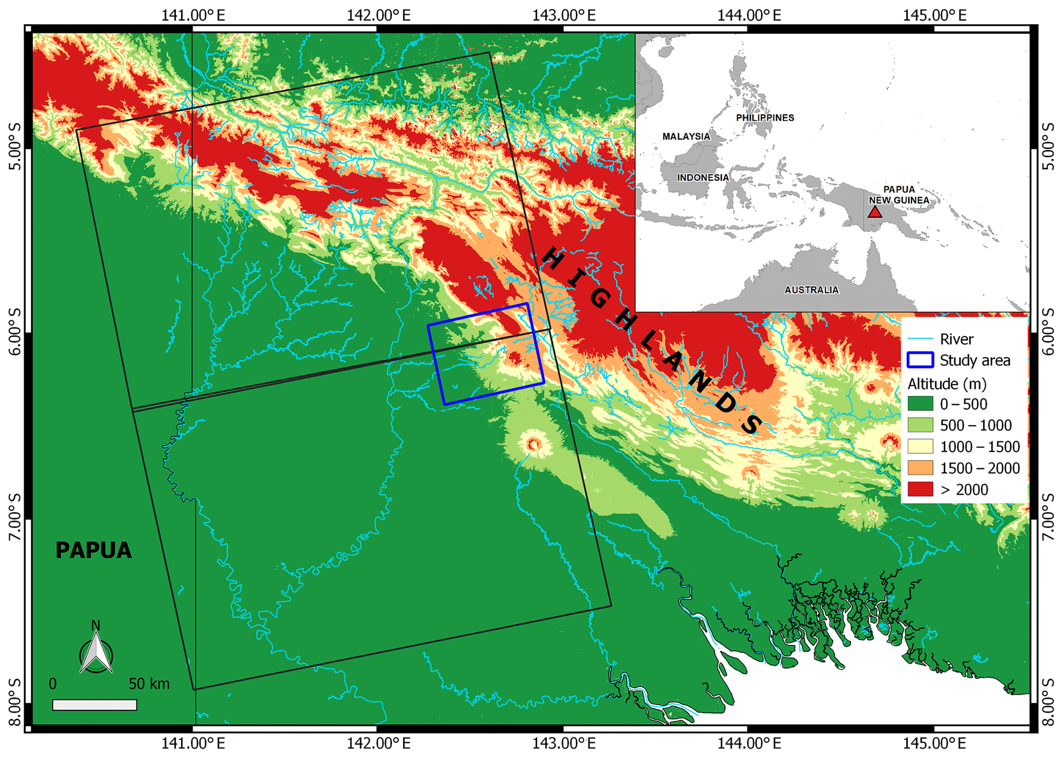
Figure 2Location of the test site. The area of interest (AoI) is highlighted with a blue rectangle on the main map and with a red triangle in the inset. The black rectangles show the spatial coverage of the used Sentinel-1 SAR images.
To test the implemented procedure, we analyzed an area of about 3000 km2 in the mountainous region close to the epicenter of the mainshock (AoI in Fig. 2), where preliminary information on landslides were available (Petley, 2018a, b).
To simulate a periodic survey covering pre- and post-earthquake periods, we downloaded 36 Sentinel-1 images from the Sentinel Data Hub (https://scihub.copernicus.eu/, last access: 24 January 2020) acquired along the satellite track no. 82 with a temporal frequency of 12 d, from 12 November 2017 to 6 June 2018. Considering that the majority of the slopes in the study area are exposed towards the west, to limit geometrical distortions in the single images and in the change detection estimation, we preferred to use IW-SLC products acquired in ascending mode, with a VV-VH polarization. Each IW product is collected with a swath characterized by a width of 250 km, subdivided in turn to three sub-swaths containing one image per polarization, consisting of a series of bursts that are processed as independent SLC images.
The downloaded images were used to perform a total of 17 change detection analyses, which resulted in likewise LR layers, with a pixel size of about 14 m. The values of the segmentation parameters were defined with an interactive manual analysis (see Sect. 2.3) by segmenting the “pre-post M7.5 earthquake” LR layer, selecting the spatial kernel size (hs) of 10 pixels (see Sect. 2.3), and setting the maximum number of iterations to 200. This size of the spatial kernel was set to 10 pixels to detect significant differences of LR values during the smoothing stage of the segmentation process, taking into account the approximate expected size of the land cover changes. In the interactive (manual) analysis, we selected bandwidth sizes (hr; see Sect. 2.3) ranging from 0.0005 to 0.016 and thresholds (th) from 0.001 to 0.016 (Fig. 3), obtaining 20 different parameter combinations. For each pair of parameters, the number of generated segments and their average size was plotted in Fig. 3. Points highlight the major impact of the hr parameter with respect to the role played by the threshold (th) parameter in defining the number of total generated segments. Below an hr value of 0.004 over-segmentation occurs, whereas for hr values equal or larger than 0.004, the number of generated segments tends to become small and constant. With the aim of avoiding over-segmentation while maintaining a reasonable average size of the segments (to be able to also delineate small patches of the terrain where changes occurred), and considering a visual inspection of the segmentation results obtained with the different combinations, we decided to run i.segment in the automatic processing chain using the following set of parameters values: hs = 10; hr = 0.004; th = 0.008; minsize = 2; iterations = 200 (see Sect. 2.3).
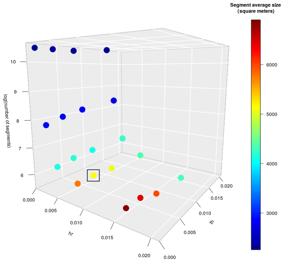
Figure 3Data analysis aimed at evaluating the best combination of bandwidth (hr) and threshold (th) values. The black rectangle identifies the selected combination.
After the segmentation of the 17 LR layers, areas affected by layover and shadowing effects were masked out in order to avoid errors in the statistical analysis described below and in the localization of potential landslides. The mask was developed in SNAP by means of the SAR Simulation Terrain Correction tool, exploiting the SRTM 1Sec DEM.
The segments with a minimum size of 5 pixels were extracted in the area of interest (an example is shown in Fig. 4d), and statistics were calculated according to the confidence intervals described in the methodology section. We decided to select only the segments with a minimum size of 5 pixels, corresponding to a minimum area of about 980 m2 (i.e., a single-pixel area roughly equal to 196 m2×5 pixels), after a general evaluation of the preliminary landslide-related images published on news websites and social networks and also considering that the detection of smaller segments in the test area was not significant at the scale of our analysis. It is worth noting that the accuracy of such a minimum area is not accurate due to the use of a geographic (and thus not projected) reference system (WGS84).
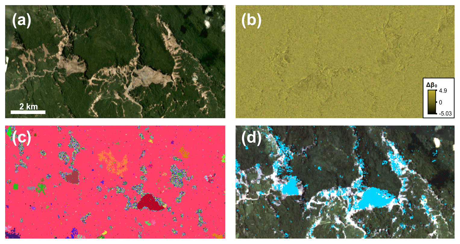
Figure 4(a) Optical image of a small sample area affected by landslides within the AoI. (b) The corresponding LR layer. (c) Output of the segmentation algorithm (obtained using the optimized hr and th values), where the different colors are random and have the sole purpose of differentiating the different segments. (d) The extracted landslide-related segments (in blue). Optical images have been downloaded from the Planet explorer application (Planet Team, 2017).

Figure 5Statistics of the segments identified for each change detection. (a) Number of segments with more than 5 pixels. (b, c) Maximum and average number of pixels per segment. Peaks of the change detections 9 and 10 indicate the occurrence of widespread land cover changes. The dashed lines show the 95∘ percentiles of the distributions (not including change detections 9 and 10).
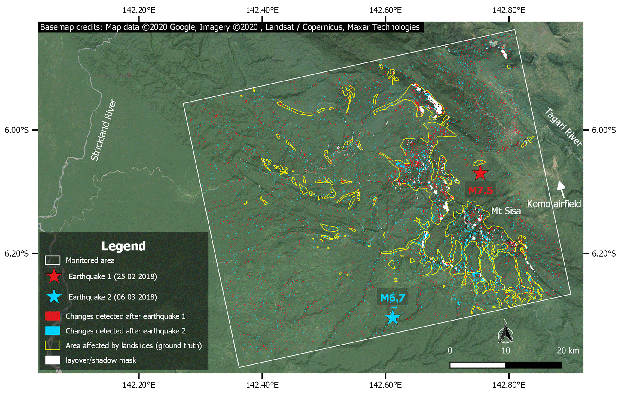
Figure 6The location of the epicenters of the two main earthquakes and the distribution of segments representing SAR amplitude changes for the change detections 9 (red) and 10 (blue). Yellow polygons are areas affected by clusters of landslides, as interpreted from optical data. The white rectangle identifies the AoI (see Fig. 2).
In Fig. 5, statistics of the selected segments are displayed for each change detection. The analysis of the histograms revealed two main peaks corresponding to change detections 9 and 10. Change detection 9 considers images acquired before and after the M7.5 earthquake, whereas change detection 10 considers the images acquired on 28 February and 12 March 2018. The first peak highlights widespread changes related to landslides that were extensively documented after the M7.5 event (Petley, 2018a). The second peak was instead unexpected and was probably due to the occurrence of further landslides triggered by the M6.7 event on 6 March 2018. In Fig. 6, segments related to these two peaks are displayed (red pixels relate to change detection 9; blue pixels relate to change detection 10). To check whether these segments were effectively located in areas characterized by a high concentration of seismically induced landslides, we analyzed optical images available on the Planet explorer application (Planet Team, 2017). By means of a visual interpretation, we identified the zones (the yellow polygons shown in Fig. 6) where clusters of landslides occurred, verifying a general accordance with the spatial distribution of both red and blue segments.
Small widespread segments outside the areas affected by landslides, mostly related to stream changes and noise, also resulted in the AoI. Similar random segments occurred in the pre- and post-event change detections, as also displayed by statistics in Fig. 5.
3.1 Statistical evidence of landslide-like segments
Evidence of the widespread land cover changes induced by the two earthquakes, as well as the timing of their occurrence, also resulted from a statistical analysis of the segment areas derived from each change detection. The comparison of some representative statistics of segment's areas related to different change detections are shown in Fig. 7. For each comparison, four types of statistics are displayed: Quantile–Quantile (Q–Q) plot, Empirical Cumulative Distribution Function (ECDF), Density plot and Frequency plot.
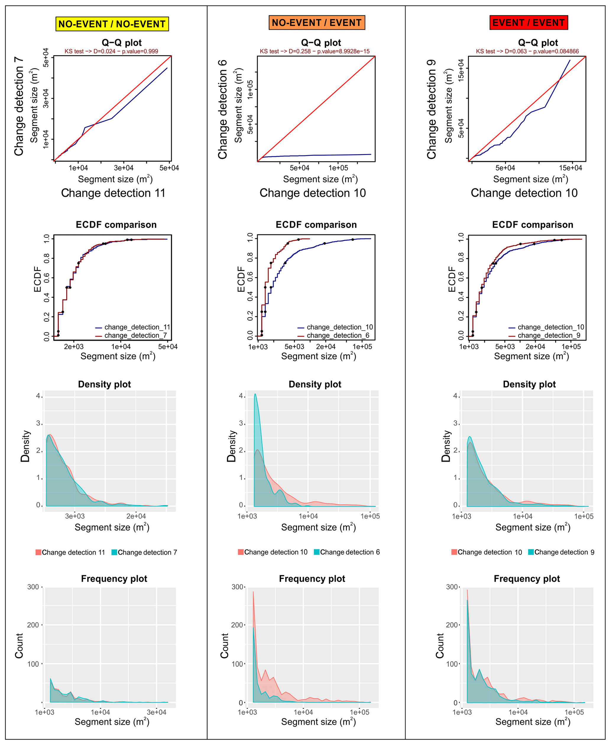
The first column in Fig. 7 compares areas of the segments resulted from the change detections 11 and 7, which we assume to not be affected by landslides triggered by the earthquake (i.e., NO-EVENT/NO-EVENT, where the term EVENT refers to the earthquake shocks); the second column shows the comparison between areas of the segments resulting from change detections 6 and 10, with the second including seismically triggered landslides (i.e., NO-EVENT/EVENT); the third column indicates the comparison between areas of the segments from change detections 9 and 10, both with landslides (i.e., EVENT/EVENT).
Clear differences can be noted between the area's distribution of segments with and without landslides (change detection 6 – change detection 10) displayed in the NO-EVENT/EVENT plots. This difference is particularly highlighted in the Q–Q plot, where the gap between the blue line representing the real distributions and the theoretical similarity condition (red line) is evident.
Considering the p values from the Kolmogorov–Smirnov tests carried out for all the 136 distribution comparisons (the combination of 17 change detections taken 2 at a time without repetition), a general similarity arises (i.e., p value > 0.05) among 81 of the 105 distributions that were not affected by landslides (NO-EVENT/NO-EVENT) (Fig. 8). On the other hand, among the 30 NO-EVENT/EVENT distributions, the majority (21/30) are different. The EVENT/EVENT distribution is instead the same (Fig. 8).
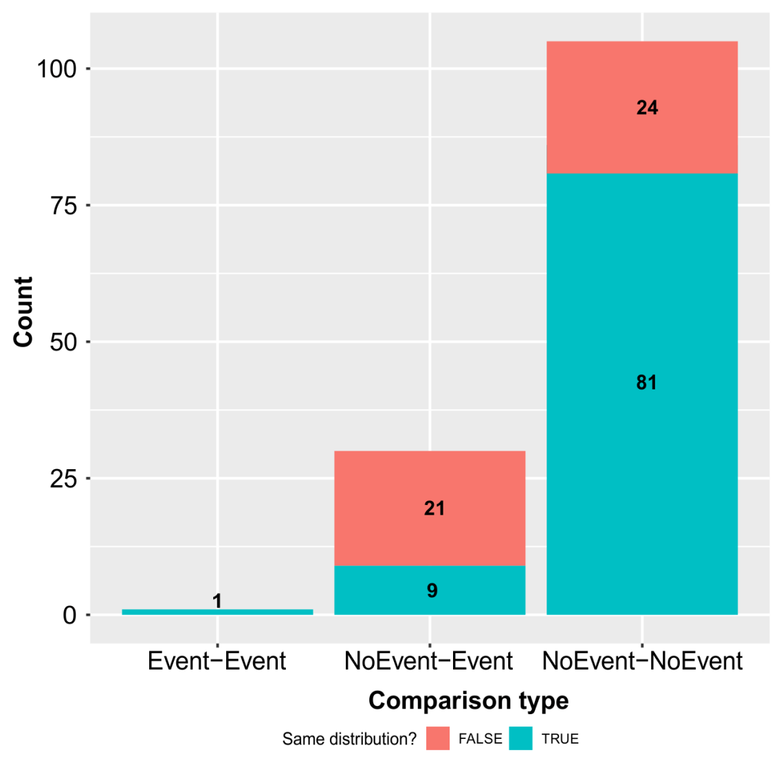
Figure 8Histogram representing the differences between all the compared segment's area distributions, calculated according to the p value of the Kolmogorov–Smirnov tests.
We have attempted to analyze the distribution of the areas of the segments derived from the change detections to verify if they followed the empirical statistical distribution of the landslide size, as described by different theoretical models (Stark and Hovius, 2001; Malamud et al., 2004; Rossi et al., 2012; Schlögel et al., 2015).
By using the tool implemented by Rossi et al. (2012) for estimating the probability distribution of landslide areas, we verified that medium and large-scale areas of segments obtained with change detections 9 and 10 followed a landslide-like behavior. In fact, the two probability distributions obtained with a Double Pareto Simplified model (Fig. 9) resulted in inverse power law decay for medium and large areas, highlighting a moderate agreement with empirical data. A rollover (inflection) in correspondence in small areas (e.g., Malamud et al., 2004), however, is not present. This could be due to a consistent detection of small changes (i.e., ∼1000 m2) ascribable to landslides and other random land cover modifications, as well as some noise. In addition, it is worth remembering that segments with areas ≤ 980 m2 were not considered.
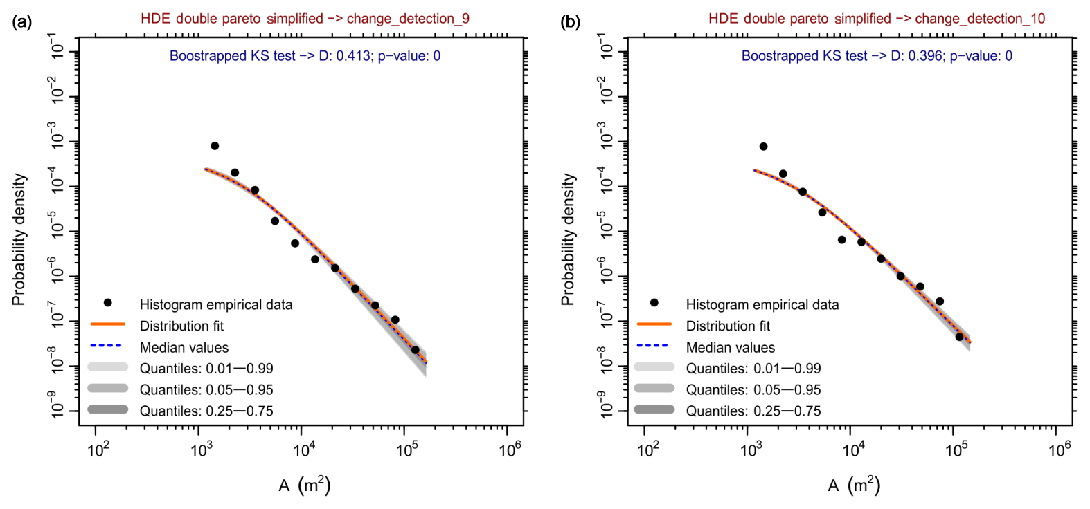
Figure 9Frequency–area distribution of segments resulting in the change detections 9 (a) and 10 (b) and fitting with a Double Pareto simplified model.
As shown in Fig. 9, the two analyses did not pass the Kolmogorov–Smirnov test (p value = 0). This may be explained by the fact that the input datasets (i.e., segments area) were not obtained with a proper landslide mapping activity, as described in Guzzetti et al. (2012), but with a procedure that is not aimed at landslide mapping operations, as clarified in the Introduction, but at identifying land cover changes also related to landslides. Despite this, results seem to be fairly consistent with curves of proper landslide inventory data (Schlögel et al., 2015).
In this article, we describe a processing chain aimed at identifying SAR amplitude changes that can be partially explained by the occurrence of mass movements. We have selected SAR data since they have the advantage of not being affected by the cloud cover disturbance. In fact, as described by Mondini et al. (2019), the use of SAR amplitude data can mitigate the cloud coverage issue and can allow for detecting landslides that otherwise might remain unknown or unnoticed for a long time. In this way, the procedure can be exploited for a “continuous” (in terms of time) slope monitoring activity, even if failures occur during long-lasting periods of precipitation and persistent cloud cover that do not allow us to use optical data for a rapid and detailed landslide recognition. In the selected study area, widespread cloud cover persisted for several weeks during and after the seismic sequence. The first cloudless optical image of the area damaged by the seismic shaking was published by the daily monitoring service delivered by © 2019 Planet Labs Inc. (https://www.planet.com/, last access: 24 January 2020) on 25 March, almost 1 month after the M7.5 mainshock that triggered numerous landslides. The high cloud persistence is quite common in Papua New Guinea, and in fact this is one of the cloudiest regions of the world, with an annual cloud frequency (proportion of days with a positive cloud flag) higher than 80 % percent (Wilson and Jets, 2016; Mondini et al., 2019). As a consequence, the use of optical data in this area, and in other mountainous regions exposed to prolonged rainfall related to monsoons, cyclones, or other persistent meteorological systems, is tricky.
The obtained results depend on the definition of the image preprocessing and segmentation parameters that should be calibrated a priori (see Sect. 2.3 and 2.4). While the geometric and radiometric corrections to the images are quite standard and well-accepted procedures, the SAR multiplicative noise filtering remains a largely discussed point in the scientific literature, and there is not a consensus on the selection of strategies. We chose the Frost filter because it has already been proven to work properly in mountainous environments (Schellenberger et al., 2012) and it was used successfully in previous studies dealing with landslides (Mondini, 2017). We acknowledge that different filters might have produced different results or requested a different tuning of the segmentation procedure. The impact of different filters on our procedure might be an interesting follow up to this work. Another improvement may consist of the use of images acquired in both ascending and descending geometries. The use of ascending images was only related to focus this first step of the work on the implementation of the entire processing chain, which we tried to simplify as much as possible. In fact, there is no doubt that combining images acquired in ascending and descending geometries can improve the quality of results, representing a nontrivial advancement of the procedure that was out of the aim of this first implementation. The a priori choice of using ascending products was based on the findings that most of the slopes in the study area are exposed towards the west, with the aim of limiting the inclusion of geometrical distortions in the change detection products.
The tuning of the segmentation parameters is the key element for identifying areas affected by significant land cover changes that are also induced by rapid slope movements. This process is event dependent, requiring a well-known landslide event that occurred in the past in the analyzed area or in zones with similar topographic and land use characteristics. In the case study described here, definite values of the segmentation parameters were obtained by segmenting the pre-post M7.5 earthquake LR layer and by testing different value combinations (Fig. 3). This may represent a limit of the proposed procedure if it is applied to different geomorphic settings without past landslide events or for identifying different types of slope failures. On the other hand, if a proper event-based tuning operation is performed, a continuous monitoring of slopes can be efficiently carried out without temporal limitations, exploiting both available pre- and post-event images, as has been done for the current case history. The described application in fact highlighted that by keeping the same parameters values, landslides and other land cover changes triggered by the M6.7 aftershock were also detected. Overlapping between the calculated segments (i.e., change detections 9 and 10) to ground truth data revealed that largest SAR amplitude changes often corresponded with landslides (Fig. 6). Further evidence was provided by the statistical distributions shown in Fig. 9, with results similar to those estimated by other landslide-related studies (Stark and Hovius, 2001; Malamud et al., 2004; Rossi et al., 2012; Schlögel et al., 2015). The segments located mostly outside the areas affected by landslides were caused instead by other land cover changes that were out of the aims of this study or by random noise effects. Segments related to these changes can be easily identified because they are composed of an average number of pixels close to 10, as detected in all the change detections, whereas segments related to landslides (i.e., change detections 9 and 10) are characterized by a higher number of pixels (Fig. 5c).
The occurrence and location of secondary failures (blue pixels in Fig. 6) were not known before our analysis because they were not reported by news and local government websites and were also missing in the maps of the Copernicus Emergency Management Service (https://emergency.copernicus.eu/mapping/list-of-components/EMSR270, last access: 24 January 2020) activated for the disaster response. The general lack of information related to these failures was likely due to a series of issues affecting both the field and the satellite surveys in the aftermath of the M=6.7 earthquake. In fact, an effective assessment in the field was impeded by the road damage also caused by the mass movements triggered by the previous major M7.5 event, whereas the use of optical satellite images was hampered by a widespread cloud cover that, as stated before, persisted during several weeks after the two main seismic shakings. The first information about the occurrence of these landslides was provided online by Petley (2018b) about 1 month later, without a clear indication of its relationship with the M6.7 earthquake. The detection of this second set of failures in areas poorly affected by previous slope movements triggered by the mainshock demonstrates the relevant usefulness of the proposed processing chain.
A suitable segmentation can hence allow us to get statistical evidence of the occurrence of event landslides. Statistical distributions of the three parameters shown in Fig. 5 provided distinctive signatures of widespread land cover changes triggered by the M7.5 mainshock and by the M6.7 aftershock. It is worth noting, however, that the 95th percentile highlighted in the plots is also exceeded by other peaks (e.g., change detection 13 in the segment count) that cannot be considered as diagnostic of landslide occurrence since they are ephemeral and are not as steady in all three plots as those of the change detections 9 and 10. In the case of small-scale landslides occurring in localized portions of a wide area, the related statistical signals may be imperceptible if these are of the same magnitude as other previous and successive signals that are not related to landslides. In cases like this, distinctive evidence of slope failures can be achieved by starting the processing chain with a smaller subset of the LR layer (i.e., monitored area).
The outcomes of this study represent a concrete example of how to exploit the relevant advantages of open-source software with a command line interface (i.e., SNAP and GRASS GIS) to implement automatic processing chains. Moreover, the proposed methodology can be properly adopted to monitor areas on the order of thousands of square kilometers if powerful hardware resources are available. In fact, the preprocessing and segmentation steps require significant amounts of calculation power and memory. It is well known that the Mean Shift is a time-consuming algorithm for large datasets (Wu and Yang, 2007) and that convergence for large areas can be reached in dozens of hours. Segmentation times are proportional to the dimensions of the monitored area and to the selected spatial kernel size (hs).
A final remark concerns the occurrence of landslides in the study area. Generally, landslides in the mountainous sectors of Papua New Guinea are very common processes. Earthquakes with a magnitude greater than 5 are among the dominant factors triggering widespread landslides. According to Robbins and Petterson (2015), such earthquakes occur regularly in the country, but records of the triggered landslides are surprisingly lacking. The lack of systematic reporting and the remoteness of communities affected by such events, also impeded an adequate characterization of landslide hazard and risk (Blong, 1986). Robbins et al. (2013) stated that landslides occur annually, and failures tend to range from few cubic meters of material to mass movements with estimated volumes of 1.8×10⁹ m3, varying from debris slides, avalanches and flows to translational and rotational slides. In this framework, the landslide detection procedure described in the article may result in a relevant tool for local authorities of countries characterized by extensive remote areas repeatedly affected by slope failures, and for the humanitarian organizations operating in response to geohydrological disasters.
This study presents a procedure aimed at supporting the detection of landslides inducing sharp land cover changes on vast mountainous areas. It is based on SAR data acquired systematically by the Sentinel-1 satellites. The computation of the LR index and segmentation of the consequent raster layers allow for detecting areas affected by multi-temporal variations of the radar backscattered signal. Among them, areas potentially related to rapidly moving landslides can be identified with a robust statistical analysis. The performance of the implemented procedure was tested in back analysis in an area of about 3000 km2 in Papua New Guinea. Here, in 2018, two consecutive earthquakes (M7.5 and M6.7) triggered widespread slope failures causing more than 100 fatalities and severe damage to roads and buildings. The simulation of a multi-temporal survey of about 7 months, before and after the earthquakes, revealed the ability of the implemented procedure to detect statistical evidence of significant land cover changes in correspondence with the two events. Moreover, results demonstrated that the zones characterized by significant backscattering changes resulted in a reasonable agreement with those affected by landslides, as compared to the ground truth data.
The study highlights advantages of free SAR products that may guide the scientific community and the local authorities to develop archives of freely accessible data suitable for implementing streamlines of information aimed at monitoring natural and urbanized areas. As demonstrated in the case study, the proposed procedure has the potential to be a valid support in landslide emergency management, providing relevant information in near real time for civil protection authorities and scientists involved in the emergency response. Future improvements may limit the user decisions in the model parameterization, optimizing the processing times and refining the filtering of landslide-related changes by also considering geological and geomorphological factors.
Copernicus Sentinel-1 data have been downloaded from the Copernicus Open Access Hub (https://scihub.copernicus.eu, Copernicus, 2020).
GE and IM implemented the proposed procedure. ACM designed the preprocessing of SAR images. GE and IM designed the segmentation procedure. GE and IM carried out the experiments. GE wrote the first draft of the manuscript. MR and GE carried out the statistics for the landslide-like segments. IM, GE and PR analyzed the results. GE, SS, IM and PR improved the final version of the manuscript.
The authors declare that they have no conflict of interest.
This article is part of the special issue “Groundbreaking technologies, big data, and innovation for disaster risk modelling and reduction”. It is not associated with a conference.
The research was developed in the framework of the STRESS (Strategies, Tools and new data for REsilient Smart Societies) project, focusing on designing, implementing and testing of a Spatial Information Infrastructure, enabling the provision of new data and tools to spatial planners and risk managers in order to improve susceptibility, hazard and impact assessments of geohydrological phenomena (http://www.idpa.cnr.it/progetti_STRESS_ufficiale.html, last access: 24 January 2020). We are grateful to Chaoying Zhao, Pierluigi Confuorto and the anonymous referee for the constructive reviews and useful suggestions.
This research has been supported by the Fondazione Cariplo (grant no. 2016-0766).
This paper was edited by Carmine Galasso and reviewed by Pierluigi Confuorto and one anonymous referee.
Alvioli, M., Mondini, A. C., Fiorucci, F., Cardinali, M., and Marchesini, I.: Topography-driven satellite imagery analysis for landslide mapping, Geomat. Nat. Haz. Risk, 9, 544–567, https://doi.org/10.1080/19475705.2018.1458050, 2018.
Blong, R. J.: Natural hazards in the Papua New Guinea highlands, Mt. Res. Dev., 6, 233–246, https://doi.org/10.2307/3673393, 1986.
Bornaetxea, T., Rossi, M., Marchesini, I., and Alvioli, M.: Effective surveyed area and its role in statistical landslide susceptibility assessments, Nat. Hazards Earth Syst. Sci., 18, 2455–2469, https://doi.org/10.5194/nhess-18-2455-2018, 2018.
Calò, F., Calcaterra, D., Iodice, A., Parise, M., and Ramondini, M.: Assessing the activity of a large landslide in southern Italy by ground-monitoring and SAR interferometric techniques, Int. J. Remote Sens., 33, 3512–3530, https://doi.org/10.1080/01431161.2011.630331, 2012.
Calvello, M., Peduto, D., and Arena, L.: Combined use of statistical and DInSAR data analyses to define the state of activity of slow-moving landslides, Landslides, 14, 473–489, https://doi.org/10.1007/s10346-016-0722-6, 2017.
Casagli, N., Frodella, W., Morelli, S., Tofani, V., Ciampalini, A., Intrieri, E., Raspini, F., Rossi, G., Tanteri, L., and Lu, P.: Spaceborne, UAV and ground-based remote sensing techniques for landslide mapping, monitoring and early warning, Geoenviron. Disast., 4, 1–23, https://doi.org/10.1186/s40677-017-0073-1, 2017.
Cigna, F., Bianchini, S., and Casagli, N.: How to assess landslide activity and intensity with persistent scatterer interferometry (PSI): the PSI-based matrix approach, Landslides, 10, 267–283, https://doi.org/10.1007/s10346-012-0335-7, 2013.
Colesanti, C. and Wasowski, J.: Investigating landslides with space-borne Synthetic Aperture Radar (SAR) interferometry, Eng. Geol., 88, 173–199, https://doi.org/10.1016/j.enggeo.2006.09.013, 2006.
Comaniciu, D. and Meer, P.: Mean shift: A robust approach toward feature space analysis, IEEE T. Pattern Anal. Mach. Intel., 24, 603–619, https://doi.org/10.1109/34.1000236, 2002.
Copernicus: Open Access Hub, https://scihub.copernicus.eu, last access: 24 January 2020.
Dai, K., Li, Z., Tomás, R., Liu, G., Yu, B., Wang, X., Cheng, H., Chen, J., and Stockamp, J.: Monitoring activity at the Daguangbao mega-landslide (China) using Sentinel-1 TOPS time series interferometry, Remote Sens. Environ., 186, 501–513, https://doi.org/10.1016/j.rse.2016.09.009, 2016.
El-Darymli, K., McGuire, P., Gill, E., Power, D., and Moloney, C.: Understanding the significance of radiometric calibration for synthetic aperture radar imagery, in: Can. Conf. Electr. Comput. Eng., May 2014, Toronto, ON, Canada, https://doi.org/10.1109/CCECE.2014.6901104, 2014.
ESA: Thermal Denoising of Products Generated by the S-1 IPF, available at: https://sentinels.copernicus.eu/documents/247904/2142675/Thermal-Denoising-of-Products-Generated-by-Sentinel-1-IPF (last access: 4 January 2020), 2017.
ESA: Level-1 SLC Products, available at: https://sentinel.esa.int/web/sentinel/user-guides/sentinel-1-sar/product-types-processing-levels/level-1 (last access: 4 January 2020), 2018.
Fiorucci, F., Cardinali, M., Carlà, R., Rossi, M., Mondini, A. C., Santurri, L., Ardizzone, F., and Guzzetti, F.: Seasonal landslides mapping and estimation of landslide mobilization rates using aerial and satellite images, Geomorphology, 129, 59–70, https://doi.org/10.1016/j.geomorph.2011.01.013, 2011.
Frost, V. S., Stiles, J. A., Shanmugan, K. S., and Holtzman, J. C.: A Model for Radar Images and Its Application to Adaptive Digital Filtering of Multiplicative Noise, IEEE T. Pattern Anal. Mach. Intel., PAMI-4, 157–166, 1982.
Gabriel, A. K., Goldstein, R. M., and Zebker, H. A.: Mapping small elevation changes over large areas: differential radar interferometry, J. Geophys. Res., 94, 9183–9191, https://doi.org/10.1029/JB094iB07p09183, 1989.
Guzzetti, F., Cardinali, M., Reichenbach, P., and Carrara, A.: Comparing landslide maps: a case study in the upper Tiber River Basin, Central Italy, Environ. Manage., 25, 247–363, https://doi.org/10.1007/s002679910020, 2000.
Guzzetti, F., Mondini, A. C., Cardinali, M., Fiorucci, F., Santangelo, M., and Chang, K. T.: Landslide inventory maps: New tools for an old problem, Earth-Sci. Rev., 112, 42–66, https://doi.org/10.1016/j.earscirev.2012.02.001, 2012.
IFRC – International Federation of Red Cross and Red Crescent Societies: Emergency Plan of Action Operation Final Report – Papua New Guinea: earthquake, available at: https://reliefweb.int/sites/reliefweb.int/files/resources/MDRPG008dfr_0.pdf (last access: 24 January 2020), 2018.
Intrieri, E., Raspini, F., Fumagalli, A., Lu, P., Del Conte, S., Farina, P., Allievi, J., Ferretti, A., and Casagli, N.: The Maoxian landslide as seen from space: detecting precursors of failure with Sentinel-1 data, Landslides, 15, 123–133, https://doi.org/10.1007/s10346-017-0915-7, 2018.
Kersten, Valgur, M., Marcel, W., Jonas, Delucchi, L., unnic, Kinyanjui, L. K., Schlump, martinber, Baier, G., Keller, G., and Castro, C.: sentinelsat/sentinelsat: v0.12.2 (Version v0.12.2), Zenodo, https://doi.org/10.5281/zenodo.1293758, 2018.
Konishi, T. and Suga, Y.: Landslide detection using COSMO-SkyMed images: A case study of a landslide event on Kii Peninsula, Japan, Eur. J. Remote Sens., 51, 205–221, https://doi.org/10.1080/22797254.2017.1418185, 2018.
Li, N., Wang, R., Deng, Y., Liu, Y., Li, B., Wang, C., and Balz, T.: Unsupervised polarimetric synthetic aperture radar classification of large-scale landslides caused by Wenchuan earthquake in hue-saturation-intensity color space, J. Appl. Remote Sens., 8, 083595, https://doi.org/10.1117/1.JRS.8.083595, 2014.
Ma, H. R., Cheng, X., Chen, L., Zhang, H., and Xiong, H.: Automatic identification of shallow landslides based on Worldview2 remote sensing images, J. Appl. Remote Sens., 10, 016008, https://doi.org/10.1117/1.JRS.10.016008, 2016.
Malamud, B. D., Turcotte, D. L., Guzzetti, F., and Reichenbach, P.: Landslide inventories and their statistical properties, Earth Surf. Proc. Land., 29, 687–711, https://doi.org/10.1002/esp.1064, 2004.
Marchesini, I., Ardizzone, F., Alvioli, M., Rossi, M., and Guzzetti, F.: Non-susceptible landslide areas in Italy and in the Mediterranean region, Nat. Hazards Earth Syst. Sci., 14, 2215–2231, https://doi.org/10.5194/nhess-14-2215-2014, 2014.
Martha, T. R., Kerle, N., van Westen, C. J., Jetten, V., and Kumar, K. V.: Segment optimization and data-driven thresholding for knowledge-based landslide detection by object-based image analysis, IEEE T. Geosci. Remote, 49, 4928–4943, https://doi.org/10.1109/TGRS.2011.2151866, 2011.
McCue, K., Gibson, G., and Love, D.: The Mainshock of 25 February 2018 and Aftershocks in the Central Highlands of Papua New Guinea, in: Australian Earthquake Engineering Society 2018 Conference, 16–18 November 2018, Perth, WA, 2018.
Mergili, M., Marchesini, I., Alvioli, M., Metz, M., Schneider-Muntau, B., Rossi, M., and Guzzetti, F.: A strategy for GIS-based 3-D slope stability modelling over large areas, Geosci. Model Dev., 7, 2969–2982, https://doi.org/10.5194/gmd-7-2969-2014, 2014a.
Mergili, M., Marchesini, I., Rossi, M., Guzzetti, F., and Fellin, W.: Spatially distributed three-dimensional slope stability modelling in a raster GIS, Geomorphology, 206, 178–195, https://doi.org/10.1016/j.geomorph.2013.10.008, 2014b.
Momsen, E. and Metz, M.: i.segment, available at: https://grass.osgeo.org/grass74/manuals/i.segment.html (last access: 7 January 2020), 2017.
Mondini, A. C.: Measures of spatial autocorrelation changes in multitemporal SAR images for event landslides detection, Remote Sens., 9, 554, https://doi.org/10.3390/rs9060554, 2017.
Mondini, A. C., Chang, K. T., and Yin, H. Y.: Combining multiple change detection indices for mapping landslides triggered by typhoons, Geomorphology, 134, 440–451, https://doi.org/10.1016/j.geomorph.2011.07.021, 2011.
Mondini, A. C., Santangelo, M., Rocchetti, M., Rossetto, E., Manconi, A., and Monserrat, O.: Sentinel-1 SAR amplitude imagery for rapid landslide detection, Remote Sens., 11, 1–25, https://doi.org/10.3390/rs11070760, 2019.
Petley, D.: An emerging crisis? Valley blocking landslides in the Papua New Guinea highlands, available at: https://blogs.agu.org/landslideblog/2018/02/28/papua-new-guinea-crisis/ (last access: 24 January 2020), 2018a.
Petley, D.: Papua New Guinea earthquake – continued landslide impacts, available at: https://blogs.agu.org/landslideblog/2018/03/14/papua-new-guinea-earthquake-3/ (last access: 24 January 2020), 2018b.
Planet Team: Planet Application Program Interface: In Space for Life on Earth, San Francisco, CA, available at: https://api.planet.com (last access: 24 January 2020), 2017.
Plank, S.: Rapid damage assessment by means of multi-temporal SAR – A comprehensive review and outlook to Sentinel-1, Remote Sens., 6, 4870–4906, https://doi.org/10.3390/rs6064870, 2014.
Plank, S., Twele, A., and Martinis, S.: Landslide mapping in vegetated areas using change detection based on optical and polarimetric SAR data, Remote Sens., 8, 307, https://doi.org/10.3390/rs8040307, 2016.
Raspini, F., Bardi, F., Bianchini, S., Ciampalini, A., Del Ventisette, C., Farina, P., Ferrigno, F., Solari, L., and Casagli, N.: The contribution of satellite SAR-derived displacement measurements in landslide risk management practices, Nat. Hazards, 86, 327–351, https://doi.org/10.1007/s11069-016-2691-4, 2017.
Reichenbach, P., Rossi, M., Malamud, B. D., Mihir, M., and Guzzetti, F.: A review of statistically-based landslide susceptibility models, Earth-Sci. Rev., 180, 60–91, https://doi.org/10.1016/j.earscirev.2018.03.001, 2018.
Robbins, J. C. and Petterson, M. G.: Landslide inventory development in a data sparse region: spatial and temporal characteristics of landslides in Papua New Guinea, Nat. Hazards Earth Syst. Sci. Discuss., 3, 4871–4917, https://doi.org/10.5194/nhessd-3-4871-2015, 2015.
Robbins, J. C., Petterson, M. G., Mylne, K., and Espi, J. O.: Tumbi Landslide, Papua New Guinea: Rainfall induced?, Landslides, 10, 673–684, https://doi.org/10.1007/s10346-013-0422-4, 2013.
Rossi, M. and Reichenbach, P.: LAND-SE: a software for statistically based landslide susceptibility zonation, version 1.0, Geosci. Model Dev., 9, 3533–3543, https://doi.org/10.5194/gmd-9-3533-2016, 2016.
Rossi, M., Ardizzone, F., Cardinali, M., Fiorucci, F., Marchesini, I., Mondini, A. C., Santangelo, M., Ghosh, S., Riguer, D. E. L., Lahousse, T., Chang, K. T., and Guzzetti, F.: A tool for the estimation of the distribution of landslide area in R, Geophys. Res. Abstr., 14, EGU2012-9438-1, 2012.
Salvi, S., Stramondo, S., Funning, G. J., Ferretti, A., Sarti, F, and Mouratidis, A.: The Sentinel-1 mission for the improvement of the scientific understanding and the operational monitoring of the seismic cycle, Remote Sens. Environ., 120, 164–174, https://doi.org/10.1016/j.rse.2011.09.029, 2012.
Santangelo, M., Marchesini, I., Bucci, F., Cardinali, M., Fiorucci, F., and Guzzetti, F.: An approach to reduce mapping errors in the production of landslide inventory maps, Nat. Hazards Earth Syst. Sci., 15, 2111–2126, https://doi.org/10.5194/nhess-15-2111-2015, 2015.
Schellenberger, T., Ventura, B., Zebisch, M., and Notarnicola, C.: Wet Snow Cover Mapping Algorithm Based on Multitemporal COSMO-SkyMed X-Band SAR Images, IEEE J. Sel. Top. Appl., 5, 1045–1053, https://doi.org/10.1109/JSTARS.2012.2190720, 2012.
Schlögel, R., Malet, J.-P., Reichenbach, P., Remaître, A., and Doubre, C.: Analysis of a landslide multi-date inventory in a complex mountain landscape: the Ubaye valley case study, Nat. Hazards Earth Syst. Sci., 15, 2369–2389, https://doi.org/10.5194/nhess-15-2369-2015, 2015.
Shimada, M., Watanabe, M., Kawano, N., Ohki, M., Motooka, T., and Wada, Y.: Detecting Mountainous Landslides by SAR Polarimetry: A Comparative Study Using Pi-SAR-L2 and X-band SARs, Trans. Japan Soc. Aeronaut. Sp. Sci. Aerosp. Technol. Japan, 12, Pn_9–Pn_15, https://doi.org/10.2322/tastj.12.pn_9, 2014.
Skriver, H.: Crop classification by multitemporal C- and L-band single- and dual-polarization and fully polarimetric SAR, IEEE T. Geosci. Remote, 50, 2138–2149, https://doi.org/10.1109/TGRS.2011.2172994, 2012.
Stark, C. P. and Hovius, N.: The characterization of landslide size distributions, Geophys. Res. Lett., 28, 1091–1094, https://doi.org/10.1029/2000GL008527, 2001.
Steger, S., Brenning, A., Bell, R., Petschko, H., and Glade, T.: Exploring discrepancies between quantitative validation results and the geomorphic plausibility of statistical landslide susceptibility maps, Geomorphology, 262, 8–23, https://doi.org/10.1016/j.geomorph.2016.03.015, 2016.
Tessari, G., Floris, M., and Pasquali, P.: Phase and amplitude analyses of SAR data for landslide detection and monitoring in non-urban areas located in the North-Eastern Italian pre-Alps, Environ. Earth Sci., 76, 1–11, https://doi.org/10.1007/s12665-017-6403-5, 2017.
Twele, A., Cao, W., Plank, S., and Martinis, S.: Sentinel-1-based flood mapping: a fully automated processing chain, Int. J. Remote Sens., 37, 2990–3004, https://doi.org/10.1080/01431161.2016.1192304, 2016.
USGS – United States Geological Survey: Event page of the M 7.5 Papua New Guinea earthquake occurred on February 25, 2018, available at: https://earthquake.usgs.gov/earthquakes/eventpage/us2000d7q6/executive#executive (last access: 7 January 2020), 2018.
van Westen, C. J., van Asch, T. W. J., and Soeters, R.: Landslide hazard and risk zonation – why is it still so difficult?, B. Eng. Geol. Environ., 65, 167–184, https://doi.org/10.1007/s10064-005-0023-0, 2006.
Wilson, A. M. and Jetz, W.: Remotely Sensed High-Resolution Global Cloud Dynamics for Predicting Ecosystem and Biodiversity Distributions, PLoS Biol., 14, e1002415, https://doi.org/10.1371/journal.pbio.1002415, 2016.
Wu, K. L. and Yang, M. S.: Mean shift-based clustering, Pattern Recognit., 40, 3035–3052, https://doi.org/10.1016/j.patcog.2007.02.006, 2007.
Yamaguchi, Y.: Disaster Monitoring by Fully Polarimetric SAR Data Acquired With ALOS-PALSAR, Proc. IEEE, 100, 2851–2860, https://doi.org/10.1109/JPROC.2012.2195469, 2012.
Zhao, C., Lu, Z., Zhang, Q., and De La Fuente, J.: Large-area landslide detection and monitoring with ALOS/PALSAR imagery data over Northern California and Southern Oregon, USA, Remote Sens. Environ., 124, 348–359, https://doi.org/10.1016/j.rse.2012.05.025, 2012.
Zhao, C., Zhang, Q., Yin, Y., Lu, Z., Yang, C., Zhu, W., and Li, B.: Pre-, co-, and post- rockslide analysis with ALOS/PALSAR imagery: a case study of the Jiweishan rockslide, China, Nat. Hazards Earth Syst. Sci., 13, 2851–2861, https://doi.org/10.5194/nhess-13-2851-2013, 2013.
GPT is the Command Line Interface of the open-source software SNAP Sentinel Application Platform, version 6.0 – http://step.esa.int/main/toolboxes/snap/ (last access: 24 January 2020). The source code of SNAP is available at https://github.com/senbox-org (last access: 24 January 2020).