On snow stability interpretation of extended column test results

Snow instability tests provide valuable information regarding the stability of the snowpack. Test results are key data used to prepare public avalanche forecasts. However, to include them into operational procedures, a quantitative interpretation scheme is needed. Whereas the interpretation of the rutschblock test (RB) is well established, a similar detailed classification for the extended column test (ECT) is lacking. Therefore, we develop a four-class stability interpretation scheme. Exploring a large data set of 1719 ECTs observed at 1226 sites, often performed together with a RB in the same snow pit, and corresponding slope stability information, we revisit the existing stability interpretations and suggest a more detailed classification. In addition, we consider the interpretation of cases when two ECTs were performed in the same snow pit. Our findings confirm previous research, namely that the crack propagation propensity is the most relevant ECT result and that the loading step required to initiate a crack is of secondary importance for stability assessment. The comparison with the RB showed that the ECT classifies slope stability less reliably than the RB. In some situations, performing a second ECT may be helpful when the first test did not indicate rather unstable or stable conditions. Finally, the data clearly show that false-unstable predictions of stability tests outnumber the correct-unstable predictions in an environment where overall unstable locations are rare.

1 Introduction

Gathering information about current snow instability is crucial when evaluating the avalanche situation. However, direct evidence of instability – as recent avalanches, shooting cracks or whumpf sounds – is often lacking. When such clear indications of instability are absent, snow instability tests are widely used to obtain information on the stability of the snowpack. Such tests provide information on failure initiation and subsequent crack propagation – essential components for slab avalanche release (Schweizer et al., 2008b; van Herwijnen and Jamieson, 2007). However, performing snow instability tests is time-consuming, as they require digging a snow pit. Furthermore, considerable experience in the selection of a representative and safe site is needed, and the interpretation of test results is challenging (Schweizer and Jamieson, 2010). Alternative approaches, such as interpreting snow micro-penetrometer signals (Reuter et al., 2015), are promising but not sufficiently established yet.

Two commonly used tests to assess snow instability are the rutschblock test (RB, Föhn, 1987) and the extended column test (ECT; Simenhois and Birkeland, 2006, 2009). For both tests, which are described in greater detail in Sect. 2.1, blocks of snow are isolated from the surrounding snowpack. According to test specifications, the block is then loaded in several steps. The loading step leading to a crack in a weak layer (failure initiation) is recorded, as well as whether crack propagation across the entire block of snow occurs (crack propagation). For the RB, the interpretation of the test result is well established and involves combining failure initiation (score) and crack propagation (release type) (e.g. Schweizer, 2002; Winkler and Schweizer, 2009). In contrast, the original interpretation of ECT results considers crack propagation propensity only (Simenhois and Birkeland, 2006, 2009; Ross and Jamieson, 2008): if a loading step leads to a crack propagating across the entire column, the result is considered unstable; otherwise it is considered stable. However, Winkler and Schweizer (2009) suggested improving this binary classification by additionally considering the loading step required to initiate a crack and by considering a minimal failure layer depth leading to interpretations of ECT results as unstable, intermediate and stable. Moreover, they hypothesized that performing two tests, and considering differences in test results, may help to establish an intermediate stability class.

As the properties of the slab as well as the weak layer may vary on a slope (Schweizer et al., 2008a), reliably estimating slope stability requires many samples (Reuter et al., 2016), and a single test result may not be indicative. Hence, it was suggested to perform more than one test, either in the same snow pit or in a distance beyond the correlation length, which is often on the order of ≤10 m (Kronholm et al., 2004). For instance, Schweizer and Bellaire (2010) analysed whether performing two pairs of compression tests (CTs) about 10 m apart improves slope stability evaluation. They suggested a sampling strategy that essentially suggests that in case the first test does not indicate instability, additional tests can reduce the number of false-stable predictions. Moreover, they reported that in 61 %–75 % of the cases the two tests in the same pit provided consistent results, and in the remaining cases either the CT score or the fracture type varied. For the ECT, several authors also noted that two tests performed adjacent to each other in the same snow pit or at several metres distance within the same small slope showed different results (Winkler and Schweizer, 2009; Hendrikx et al., 2009; Techel et al., 2016). For instance, Techel et al. (2016) reported that in 21 % of the cases the ECT fracture propagation result differed between two tests in the same snow pit. Moreover, they explored differences in the performance between the ECT and the RB with regard to slope stability evaluation and found that the RB detected more stable and unstable slopes correctly than a single ECT or two adjacent ECTs.

Both ECT and RB provide information relating to slab avalanche release. While the rutschblock test provides reliable results, the ECT is quicker to perform in the field, which probably explains why it has quickly become the most widely used instability test in North America (Birkeland and Chabot, 2012). Given the popularity of the ECT as a test to obtain snow instability information and the lack of a quantitative interpretation scheme that includes more than just two classes, our objective is to revisit the originally suggested stability interpretations and to specifically consider cases when two ECTs were performed in the same snow pit. Building on our findings, we propose a new stability classification differentiating between cases when just a single ECT and when two adjacent ECTs were performed in the same snow pit, with the goal of minimizing false-stable and false-unstable predictions. Additionally, we empirically explore the influence of the base rate frequency of unstable locations on stability test interpretation, which – if neglected – may lead to false interpretations (Ebert, 2019). We address this topic by exploring a large set of ECTs with observations of slope stability collected in Switzerland. Furthermore, ECT results are compared with concurrent RB results.

2 Data

Data were collected in 13 winters from 2006–2007 to 2018–2019 in the Swiss Alps. We explored a data set of stability test results in combination with information on slope stability and avalanche hazard.

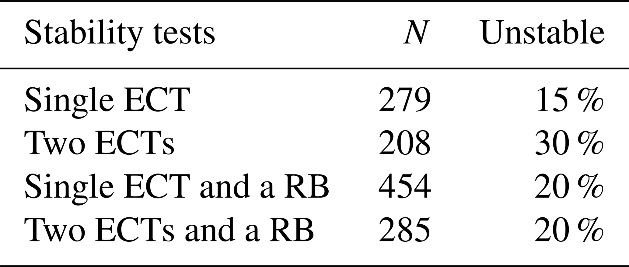
At 1226 sites, where slope stability information was available, 1719 ECT were performed (Table 1). At 487 out of the 1226 sites either one (279) or two ECTs (208) were performed (695 ECTs in total). At the other 739 sites, a RB was conducted in addition to either one (484) or two ECTs (285) in the same snow pit (1024 ECTs in total).

Table 1 Data overview with the number (N) and proportion of slopes rated as unstable.

2.1 Extended column test (ECT) and rutschblock test (RB)

At sites where ECT and RB were realized in the same snow pit, one or two ECTs were generally performed directly downslope from the RB (e.g. as described in detail in Winkler and Schweizer, 2009). If no RB was performed but two ECTs were performed, it is not known whether the ECTs were performed side by side or whether the second ECT was located directly upslope from the first ECT.

Test procedure followed observational guidelines (Greene et al., 2016). For the ECT, loading is by tapping on the shovel blade positioned on the snow surface on one side of the column of snow isolated from the surrounding snowpack (30 loading steps, Fig. 1a). For the RB, a person on skis stands or jumps on the block (six loading steps, Fig. 1b). When a crack initiates and propagates within the same weak layer across the entire column within one tap of crack initiation, it is called ECTP for the ECT; for the RB this corresponds to the release-type whole block. If the crack does not propagate within the same layer across the entire column or within one tap of crack initiation, ECTN is recorded for the ECT. Similarly, if the fracture does not propagate through the entire block, part of block or edge only are recorded as a RB release type. If no failure can be initiated including loading step 30 (ECT) or 6 (RB), these are recorded as ECTX or RB7, respectively.

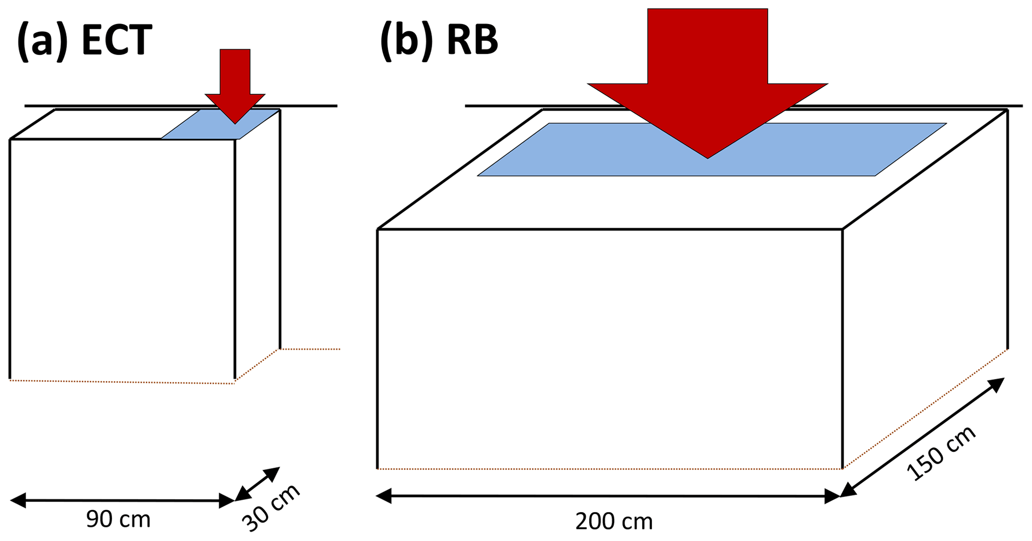
Figure 1 ECT and RB according to observational guidelines. At the back, the block of snow is isolated by cutting with either a cord or a snow saw. The light-blue area indicates the approximate area, where the skis or the shovel blade is placed. This area corresponds to the area loaded for the ECT, while the main load under the skis is exerted over a length of about 1 m (Schweizer and Camponovo, 2001). Loading is from above (arrows).

2.2 Stability classification of ECT and RB

To facilitate the distinction between the result of an instability test and the stability of a slope, we refer to test stability using four classes, 1 to 4, with class 1 being the lowest stability (poor or less) and class 4 the highest stability (good or better). In contrast, for slope stability, we use the terms unstable and stable. We chose four classes as a similar number of classes has been used for RB stability interpretation, as outlined below.

2.2.1 Extended column test (ECT)

The stability classification originally introduced by Simenhois and Birkeland (2009) (ECT_orig) suggested two stability classes: ECTN or ECTX are considered to indicate high stability (class 4), while ECTP indicates low stability (class 1).

The classification suggested by Winkler and Schweizer (2009) (ECT_w09) uses three classes:

• ECTP ≤21 – low stability (class 1)

• ECTP >21 – intermediate stability (class 2–3)

• ECTN or ECTX – high stability (class 4).

2.2.2 Rutschblock test (RB)

We classified the RB into four classes (classes 1 to 4; Fig. 2). We followed largely the RB stability classification by Techel and Pielmeier (2014), who used a simplified version of the classification used operationally by the Swiss avalanche warning service (Schweizer and Wiesinger, 2001; Schweizer, 2007). Schweizer (2007) defined five stability classes for the RB, based on the score and the release type in combination with snowpack structure, while Techel and Pielmeier (2014) relied exclusively on RB score and release type. In contrast to both these approaches, we combined the two highest classes (good or very good) into one class (class 4).

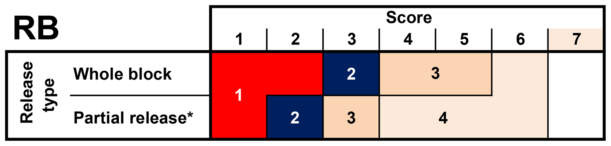
Figure 2 Classification of RB into four stability classes. ^∗ Combines release-type part of block and edge only.

Shallow weak layers (≤15 cm) are rarely associated with skier-triggered avalanches (Schweizer and Lütschg, 2001; van Herwijnen and Jamieson, 2007), which is, for instance, reflected in the threshold sum approach (Schweizer and Jamieson, 2007), a method to detect structural weaknesses in the snowpack. Schweizer and Jamieson (2007) reported the critical range for weak layers particularly susceptible to human triggering as 18–94 cm below the snow surface. Minimal depth criteria were also taken into account by Winkler and Schweizer (2009) in their comparison of different instability tests or by Techel and Pielmeier (2014), when classifying snow profiles according to snowpack structure. We addressed this by assigning stability class 4 if the failure layer was less than 10 cm below the snow surface. If there were several failures in the same test, we searched for the ECT and RB failure layer with the lowest stability class.

2.3 Slope stability classification

We classified stability tests according to observations relating to snow instability in slopes similar to the test on the day of observation, such as recent avalanche activity or signs of instability (whumpfs or shooting cracks). This information was manually extracted from the text accompanying a snow profile and/or stability test. This text contains – among other information – details regarding recent avalanche activity or signs of instability.

A slope was called unstable if any signs of instability or recent avalanche activity – natural or skier-triggered avalanches from the day of observation or the previous day – were noted on the slope where the test was carried out or on neighbouring slopes (Simenhois and Birkeland, 2006, 2009; Moner et al., 2008; Winkler and Schweizer, 2009; Techel et al., 2016).

We only called a slope stable if it was clearly stated that on the day of observation none of the before-mentioned signs were observed in the surroundings. In most cases, “surroundings” relates to observations made in the terrain covered or observed during a day of back-country touring (estimated to be approximately 10 to 25 km²; Meister, 1995; Jamieson et al., 2008).

In the following, we denote slope stability simply as stable or unstable, although this strict binary classification is not adequate. For instance, many tests were performed on slopes that were actually rated as unstable but did not fail. In other words, unstable has to be understood as a slope where the triggering probability is relatively high compared to stable where it is low.

If it was not clearly indicated when and where signs of instabilities or fresh avalanches were observed, or if this information was lacking entirely, these data were not included in our data set.

2.4 Forecast avalanche danger level

For each day and location of the snow instability test, we extracted the forecast avalanche danger level related to dry-snow conditions from the public bulletin issued at 17:00 CET and valid for the following 24 h.

3 Methods

3.1 Criteria to define ECT stability classes

We consider the following criteria as relevant when testing existing or defining new ECT stability classes:

• i.

  Stability classes should be distinctly different from each other. The criteria we rely on is the proportion of unstable slopes. Therefore, a higher stability class  should have a significantly lower proportion of unstable slopes than the neighbouring lower stability class.

• ii.

  The lowest and highest stability classes should be defined such that the rate of correctly detecting unstable and stable conditions is high, respectively; hence, the rate of false-stable and false-unstable predictions should be low, respectively. Stability classes between these two classes may represent intermediate conditions or lean towards more frequently unstable and stable conditions, permitting a higher false-stable and false-unstable rate than the rates of the two extreme stability classes.

• iii.

  The extreme classes should occur as often as possible, as the test should discriminate well between stable and unstable conditions in most cases.

To define classes based on crack propagation propensity and crack initiation (number of taps), we proceeded as follows:

1. We calculated the mean proportion of unstable slopes for moving windows of three, five and seven consecutive number of taps for ECTP and ECTN separately. ECTX was included in ECTN, treating ECTX as ECTN31.

2. We obtained thresholds for class intervals by applying unsupervised k-means clustering (R function kmeans with settings max.iter =100, nstart =100; R Core Team, 2017; Hastie et al., 2009) on the proportion of unstable slopes of the three running means (step 1). The numbers of clusters k tested were three, four and five.

3. We repeated clustering 100 times using 90 % of the data, which were randomly selected without replacement. For each of these repetitions, the cluster boundaries were noted. Based on the 100 repetitions, we report the respective most frequently observed k−1 boundaries, together with the second most frequent boundary.

4. To verify whether the classes found by the clustering algorithm were distinctly different (criterion i), we compared the proportion of unstable slopes between clusters using a two-proportion z test (prop.test; R Core Team, 2017). We considered p values ≤0.05 as significant.

   In almost all cases, we used a one-sided test with the null hypothesis H₀ being H₀: prop.(A) ≤ prop.(B) (or its inverse), where “prop.” is the proportion of unstable slopes in the respective cluster A or B. The alternative hypothesis H_a would then be H_a: prop.(A) > prop.(B) (or its inverse).

5. For clusters not leading to a significant reduction in the proportion of unstable slopes, we tested a range of thresholds (±3 taps within the threshold indicated by the clustering algorithm) to find a threshold maximizing the difference between cluster centres and leading to significant differences (p≤0.05) in the proportion of unstable slopes (criterion ii). If no such threshold could be found, clusters were merged.

Throughout this paper, we report p values in four classes (p>0.05, p≤0.05 when $p=[\mathrm{0.05},\mathrm{0.01}[$, p≤0.01 when $p=[\mathrm{0.01},\mathrm{0.001}[$ and p≤0.001).

3.2 Assessing the performance of stability tests and their classification

When the predictive power or predictive validity of a test is assessed, it is compared to a reference standard, here the slope stability classified as either unstable or stable. The usefulness of instability test results is generally assessed by considering only two categories related to unstable and stable conditions (Schweizer and Jamieson, 2010). We refer to these two outcomes as low or high stability.

There are two different contexts in which a test's adequacy is looked at. The first (a) explores whether the foundations of a test are satisfactory and the second (b) explores whether the test is useful (Trevethan, 2017).

• a.

  Most often the performance of a snow stability test is assessed from the perspective of the reference group (Schweizer and Jamieson, 2010), i.e. what proportion of unstable slopes are detected by the stability test. The two relevant measures addressing this context are the sensitivity and specificity, which are considered as the benchmark for the performance:

  • The sensitivity of a test is the probability of correctly identifying an unstable slope from the slopes that are known to be unstable. Considering a frequency table (Table 2), the sensitivity, or probability of detection (POD), is calculated as follows (Trevethan, 2017).

    $$\mathrm{Sensitivity}\left(\mathrm{POD}\right)={\displaystyle \frac{a}{a+c}}$$

  • The specificity of a test is the probability of correctly identifying a stable slope from the slopes that are known to be stable. It is also referred to as the probability of non-detection (PON).

    $$\mathrm{Specificity}\left(\mathrm{PON}\right)={\displaystyle \frac{d}{b+d}}$$

  Ideally, both sensitivity and specificity are high, which means that most unstable and most stable slopes are detected. However, missing unstable situations can have more severe consequences, and therefore it is assumed that first of all the sensitivity should be high. Nonetheless, a comparably low specificity will decrease a test's credibility.

• b.

  The second context focuses on the ability of a test to correctly indicate slope stability; i.e. if the test result indicates low stability, how often is the slope in fact unstable? This aspect has only rarely been explored for snow instability tests (e.g by Ebert, 2019, from a Bayesian viewpoint) and is generally assessed using two metrics:

  • The positive predictive value (PPV) is the proportion of unstable slopes, given that a test result indicates instability (a low-stability class).

    $$\mathrm{PPV}={\displaystyle \frac{a}{a+b}}$$

  • The negative predictive value (NPV) is the proportion of stable slopes, given that a test result indicates stability (a high-stability class).

    $$\mathrm{NPV}={\displaystyle \frac{d}{c+d}}$$

  In the following, we will use PPV and 1−NPV in the sense that it reflects the proportion of unstable slopes given a specific test result in a setting with up to four test outcomes (classes 1 to 4), which we term the proportion of unstable slopes. PPV and NPV depend strongly on to the frequency of unstable and stable slopes in the data set (Brenner and Gefeller, 1997). Thus keeping the base rate the same when making comparisons across tests and stability classifications is essential.

  To demonstrate the effect variations in the frequency of unstable and stable slopes have on predictive values like PPV or 1−NPV, we additionally explored this effect for tests observed when either danger level 1 (low), 2 (moderate), or 3 (considerable) were forecast.

Table 2 A 2×2 frequency table cross-tabulating slope stability and test results. A positive test result indicates low stability, a negative test result high stability.

3.3 Base rate for proportion of unstable and stable slopes

As outlined before, the proportion of unstable slopes varied within our data set: we noted a bias towards more frequently observing two ECTs when slope stability was considered unstable (30 %). For a single ECT, only 15 % of the tests were observed in unstable slopes (Table 1). To balance out this mismatch when comparing two ECT results to a single ECT or RB (20 % unstable), we created equivalent data sets for a single ECT and RB containing the same proportion of tests collected on unstable and stable slopes as found for the data set of two ECTs. For this, we randomly sampled an appropriate number of single ECTs and RBs observed on stable slopes (i.e. we reduced the number of stable cases) and combined these with all the tests observed on unstable slopes. We repeated this procedure 100 times. We report only the mean values of these 100 repetitions and calculated p values (prop.test) for these mean proportions and the original number of cases in the data set.

The base rate proportion with 30 % tests on unstable and 70 % on stable slopes was used throughout this paper, except in Sect. 4.5, where we evaluate the effect of different base rates.

3.4 Selecting ECT from snow pits with two ECT

For snow pits with two adjacent ECTs, we randomly selected one ECT when exploring single ECT data or the relationship between the number of taps and slope stability. As before, this procedure was repeated 100 times. The respective statistic, generally the mean proportion of unstable slopes, was calculated based on the 100 repetitions.

4 Results

4.1 Comparing existing stability classifications

We first consider the results for a single ECT. The original stability classification ECT_orig led to significantly different proportions of unstable slopes for the two stability classes (0.48 vs. 0.19, p<0.001, Fig. 3a). The ECT_w09 classification, with three different classes, showed significantly different proportions of unstable slopes between the lowest and the intermediate class (0.55 vs. 0.23, p≤0.001) but not between the intermediate and the highest class (0.23 and 0.19, p>0.05). Although ECT_w09 class 1 had a larger proportion of unstable slopes than ECT_orig class 1, the difference was not significant (p>0.05).

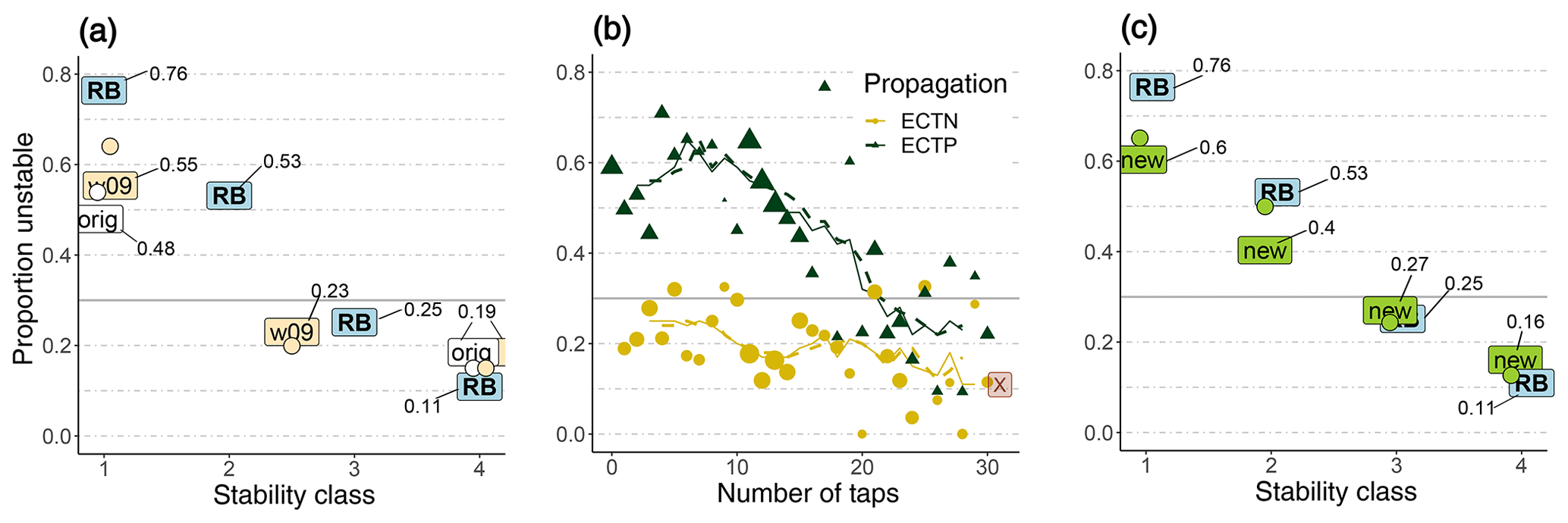
Figure 3 Proportion of unstable slopes (y axes) for (a) the two existing ECT stability classifications (ECT_orig, ECT_w09) and the RB, (b) the number of taps stratified by propagation, and (c) the classification using the ECT_new together with the RB as in panel (a). (a, c) Single ECT results are indicated by the respective text labels; the two ECTs resulting in the same stability class are indicated by circles. For a single ECT and RB, additionally the actual values for the proportion of unstable slopes are indicated. (b) The lines represent the mean proportion of unstable slopes calculated for moving windows including five or seven consecutive numbers of taps. (a–c) The 30 % unstable and 70 % stable slopes were used (i.e. the grey line shows the base rate proportion of unstable slopes).

Considering the results obtained from two adjacent ECTs resulting in the same stability class 1, between 0.54 (ECT_orig) and 0.64 (ECT_w09) of the slopes were unstable. Although the proportion of unstable slopes was higher by 0.06 to 0.09 than for a single ECT, this difference was not significant (p>0.05). When both ECTs indicated the highest stability class, the proportion of unstable slopes was 0.15, which is not significantly different than for a single ECT resulting in this stability class (0.19, p>0.05). When one test resulted in the lowest and the other in the intermediate ECT_w09 class, a proportion of 0.21 of the slopes were unstable. While this was clearly less than when both resulted in ECT_w09 class 1 (p<0.05), it was not significantly different than two ECT with ECT_w09 class 4 (0.15, p>0.05).

Regardless of whether a single ECT or two ECTs were considered, the ECT_w09 classification had a 0.07–0.08 larger proportion of unstable slopes for stability class 1 than the ECT_orig classification. For stability class 4 there was no difference, as the definition for this class is identical.

The sensitivity was higher for ECT_orig (0.62) than for ECT_w09 (class 1: 0.55, Fig. 4a and b). However, this comes at the cost of a high false-alarm rate (1−specificity) for ECT_orig (0.29), which is considerably higher than for ECT_w09 (0.19).

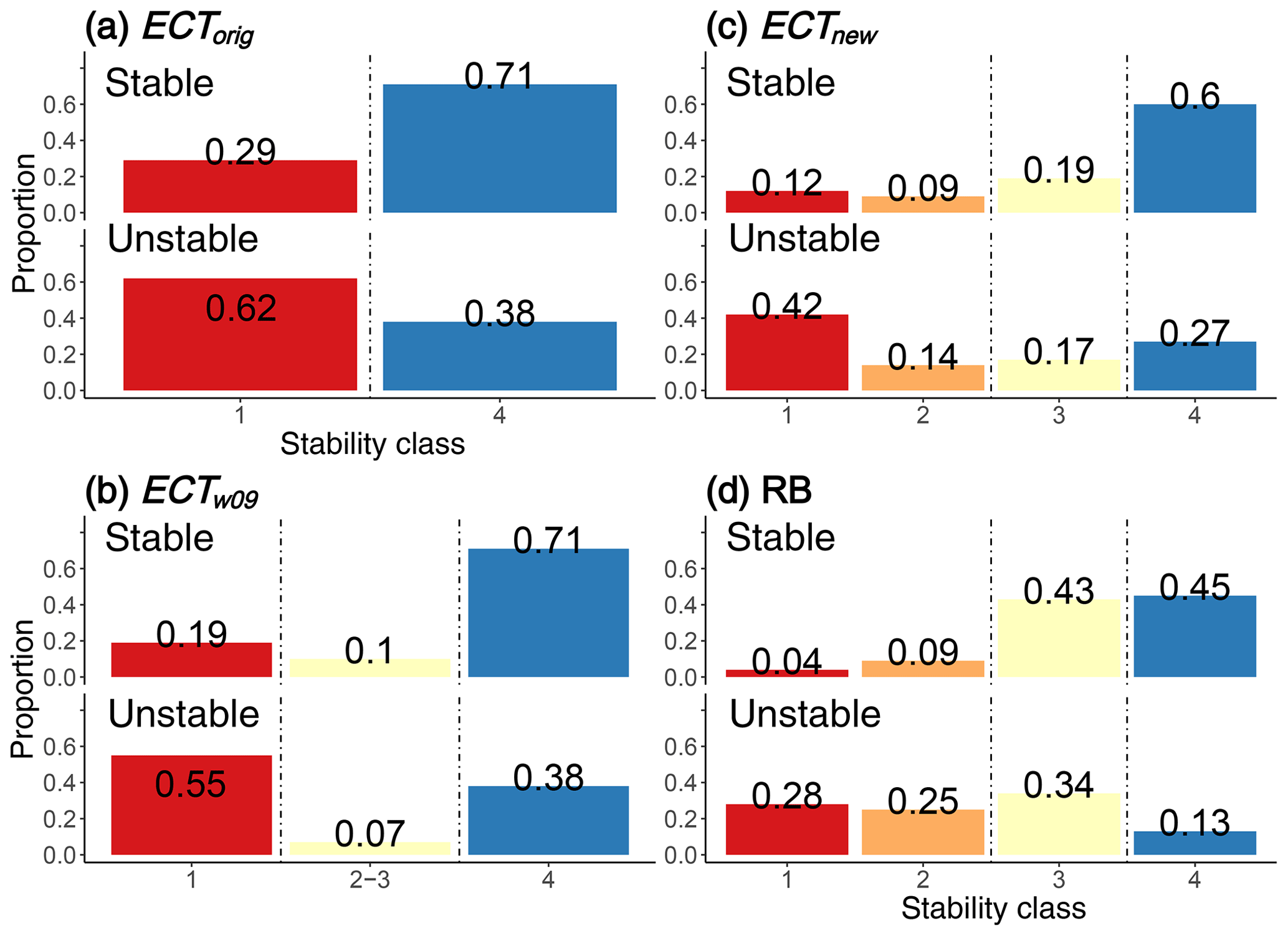
Figure 4 Distribution of stability classes by slope stability for the different stability test and classification approaches (a) with two classes (ECT_orig), (b) with three classes (ECT_w09) and (c, d) with four classes (ECT_new and RB, respectively). The vertical dashed lines indicate the thresholds when the primary slope stability associated with a test result changed from one slope stability to the other. Reading subfigures row-wise provides an indication of POD and PON. Comparing proportions column-wise corresponds to a base rate of 0.5. If no clear prevalence was observed, the stability class is considered intermediate (light yellow colour). Stability classes were considered to have no clear prevalence when the ratio of the proportion of unstable cases to the combined proportions of unstable and stable was between 0.4 and 0.6. As an example, for RB stability class 3 this ratio would be $\mathrm{0.34}/(\mathrm{0.34}+\mathrm{0.43})$.

The optimal balance between achieving a high sensitivity and a low false-alarm rate was found to be at ECTP≤21 (R library pROC; Robin et al., 2011), exactly the threshold suggested by Winkler and Schweizer (2009).

4.2 Clustering ECT results by accounting for failure initiation and crack propagation

So far, we explored existing classifications. Now, we focus on the respective lowest number of taps stratified by propagating (ECTP) and non-propagating (ECTN) results. If in the same test for different weak layers ECTN and ECTP were observed, only ECTP with the lowest number of taps was considered.

As can be seen in Fig. 3b, the proportion of unstable slopes was higher for ECTP compared to ECTN, regardless of the number of taps and in line with the original stability classification ECT_orig. However, a notable drop in the proportion of unstable slopes between about 10 and 25 taps is obvious (ECTP, from about 0.6 to almost 0.25).

Clustering the ECT results shown in Fig. 3b with the number of clusters k set to three, four and five, and repeating the clustering 100 times (refer to Sect. 3.1 for details), each time with 90 % of the data, split the data at similar thresholds. In the following, we show the results for the two most frequent cluster thresholds obtained for k=4. The frequency of the respective cluster threshold was selected in the 100 repetitions is shown in brackets:

• ECTP ≤14 (48 %), ECTP ≤13 (36 %)

• ECTP ≤20 (37 %), ECTP ≤18 (36 %)

• ECTN ≤10 (29 %), ECTN ≤9 (22 %).

Setting k to 3 resulted in clusters being divided at ECTP ≤14 and at ECTP ≤21; k=5 resulted in cluster thresholds ECTP ≤9, ECTP ≤14, ECTP ≤20 and ECTN ≤10. The second most frequent threshold was almost always within ±1 tap of those indicated before. Applying the same approach with 80 % of the data (rather than with 90 %) resulted in very similar class thresholds (see Supplement). To maximize the difference in the proportion of unstable slopes between classes, we varied the thresholds defining clusters by testing ±3 taps. The following four stability classes for a single ECT (ECT_new) in combination with the depth of the failure plane criterion were obtained (p values indicate whether the proportion of unstable slopes differed in relation to the previously described group):

1. ECTP ≤13 captures test results with the largest proportion of unstable slopes. The proportion of unstable slopes (0.6) was double the base rate (0.3).

2. ECTP >13 and ECTP ≤22 (proportion of unstable slopes =0.4, p≤0.05) indicate the transition from a high proportion (0.6, for ECTP ≤13) to a lower proportion of unstable slopes (0.27, for ECTP >22). However, the mean proportion of unstable slopes was still higher than the base rate.

3. ECTP >22 or ECTN ≤10 (0.27, p≤0.01) indicate that the proportion of unstable slopes was lower than the base rate.

4. ECTN >10 or ECTX (0.16, p≤0.05) captures test results corresponding to the lowest proportions of unstable slopes (about half the base rate).

4.3 Evaluating the new ECT stability classification

4.3.1 Stability classification for a single ECT

The ECT_new classification showed continually and significantly decreasing proportions of unstable slopes with increasing stability class (0.6, 0.4, 0.27 and 0.16 for classes 1 to 4, respectively, p≤0.01, Fig. 3c). The lowest ECT_new class had a larger proportion of unstable slopes (0.6) than the lowest classes for ECT_w09 (0.55) or ECT_orig (0.48), though this was only significant compared to ECT_orig (p≤0.05). In contrast, only marginal differences were noted when comparing the proportion of unstable slopes for stability class 4 (ECT_new 0.16, ECT_orig 0.19). Considering ECT_new class 1 as an indicator of instability, the sensitivity was 0.42. When considering classes 1 and 2 together, the sensitivity increased to 0.56 (Fig. 4c).

4.3.2 Stability classification for two adjacent ECTs

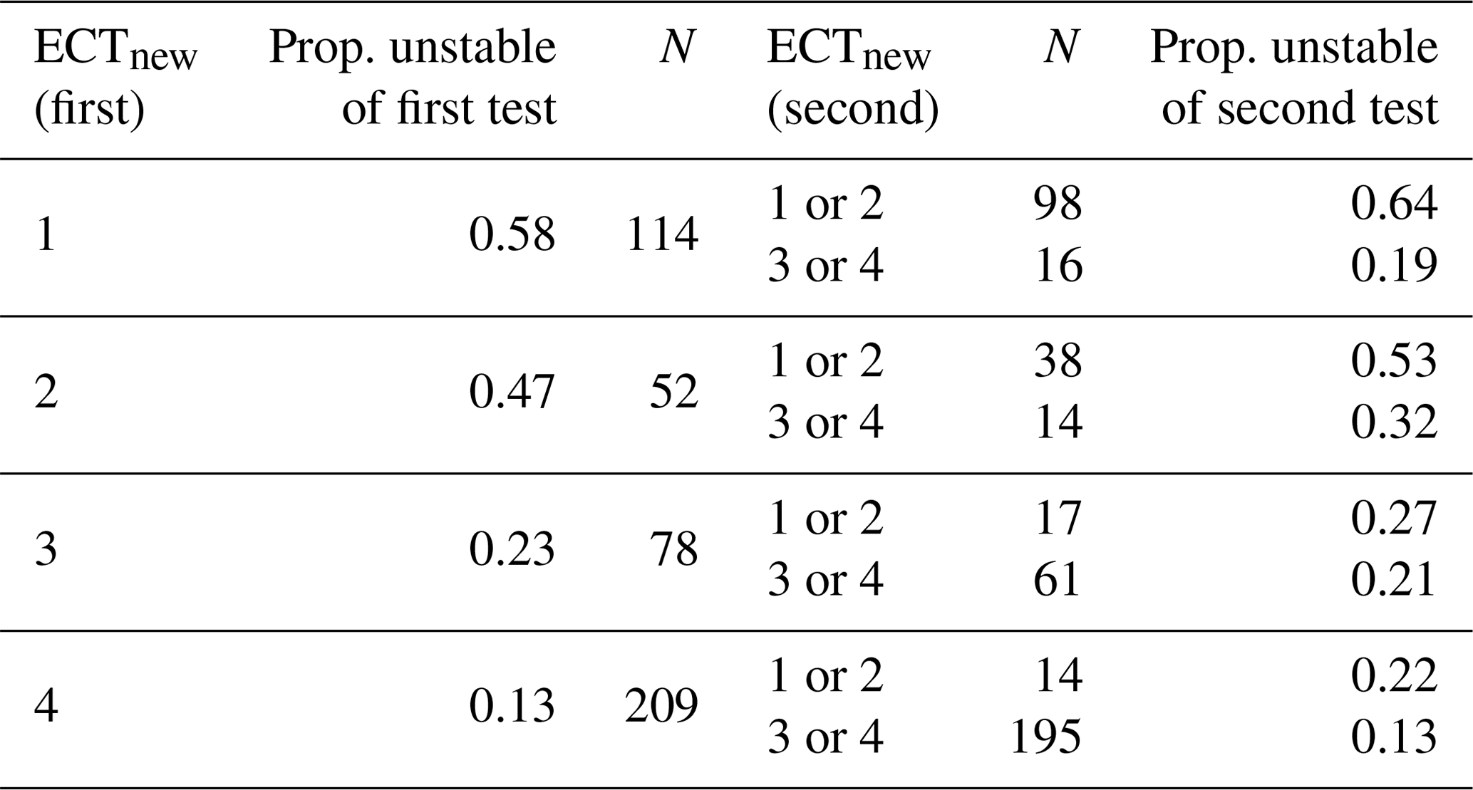
For 70 % of the time two ECTs indicated the same ECT_new class, for 19 % of the time they differed by one class and for 11 % the time they differed by two (or more) classes. Two ECTs resulting in the same ECT_new class resulted in pronounced differences in the proportion of unstable slopes for classes 1 to 4 (0.65, 0.5, 0.24 and 0.13, respectively; Fig. 3c).

Randomly picking one of the two ECTs as the first ECT yielded the proportion of unstable slopes as shown in Table 3. Additionally considering the outcome of a second ECT increased or decreased the proportion of unstable slopes for some combinations. For instance, if a first ECT resulted in either ECT_new class 1 or 4, the second test would often indicate a similar result: class ≤2 in 86 % of the cases, when the first ECT was class 1, and class ≥3 in 93 % of the cases, when the first ECT was class 4. However, if the first ECT was either ECT_new class 2 or 3, a large range of proportion of unstable slopes resulted depending on the second test result (0.21–0.53, Table 3), including some combinations resulting in the proportion of unstable slopes being close to the base rate.

Table 3 Proportion of unstable slopes when randomly selecting one of two ECTs as the first test (ECT_new (first), prop. unstable of the first test) and the number of cases (N) , and the respective proportion of unstable slopes of the second test following the outcome of the second ECT (ECT_new (second), prop. unstable of the second test).

4.4 Comparison to rutschblock test results

The proportion of unstable slopes decreased significantly with each increase in RB stability class (0.76, 0.53, 0.25 and 0.11 for classes 1 to 4, respectively; p<0.01; Fig. 3c). If a binary classification were desired, classes 1 and 2 would be considered to be indicators of instability, and classes 3 and 4 would relate to stable conditions. Employing this threshold, the sensitivity was 0.53 and the specificity 0.88 (Fig. 4d). Considering RB class 3, also termed “fair” stability (Schweizer, 2007), as an indicator of stability is, however, not truly supported by the data. This class had a proportion of unstable slopes of 0.25, which is not significantly lower than the base rate.

Comparing RB with the ECT showed that the proportion of unstable slopes for RB stability class 1 was significantly higher (p<0.01) and for class 4 about 0.05 lower (p>0.05) than for the respective ECT classifications (Fig. 3a, c). This indicates that the RB stability classes at either end of the scale captured slope stability better than the ECT results, regardless of which of the ECT classification was applied and whether a second test was performed. Figure 3a and c also highlight that RB class 2 and ECT class 1 (ECT_w09, ECT_new) had similar proportions of unstable slopes. ECT_new stability class 2 had a lower proportion of unstable slopes than RB class 2 (p<0.05) but a higher proportion than RB class 3 (p<0.05). The proportions of unstable slopes for the two highest ECT_new classes were not significantly different than for the two highest RB classes (p>0.05).

The false-alarm rate of the RB (classes 1 and 2) was lower than for any of the ECT classifications (Fig. 4). However, in our data set a comparably large proportion of RBs (0.34) indicated stability class 3 in slopes rated as unstable. This ratio is higher than for a single ECT_new class 3. However, the frequency that stability class 4 (false stable) was observed in unstable slopes was lower than for ECT_new class 4 (0.13 vs. 0.23, respectively).

The ECT_new stability class correlated significantly with the RB stability class (Spearman rank-order correlation ρ=0.43, p<0.001), a correlation which was stronger for ECT pairs resulting twice in the same ECT stability class (ρ=0.64, p<0.001). For both tests, stability class 3 was not truly related to unstable or stable conditions and may therefore be considered to represent something like fair stability.

4.5 The predictive value of stability tests – including base rate information

Now, we explore the predictive value of a stability test result as a function of the base rate proportion of unstable slopes. In our data set the base rate proportion of unstable slopes increased strongly, and in a non-linear way, with forecast danger level: for the 1108 snow pits with at least one ECT it was 0.02 for level 1 (low), 0.1 for level 2 (moderate), and 0.38 for level 3 (considerable) (Table 4).

Table 4 Proportion of unstable slopes for ECT_new and RB class 1, classes 1 and 2 combined, and class 4, stratified by regional forecast danger level (D_RF).

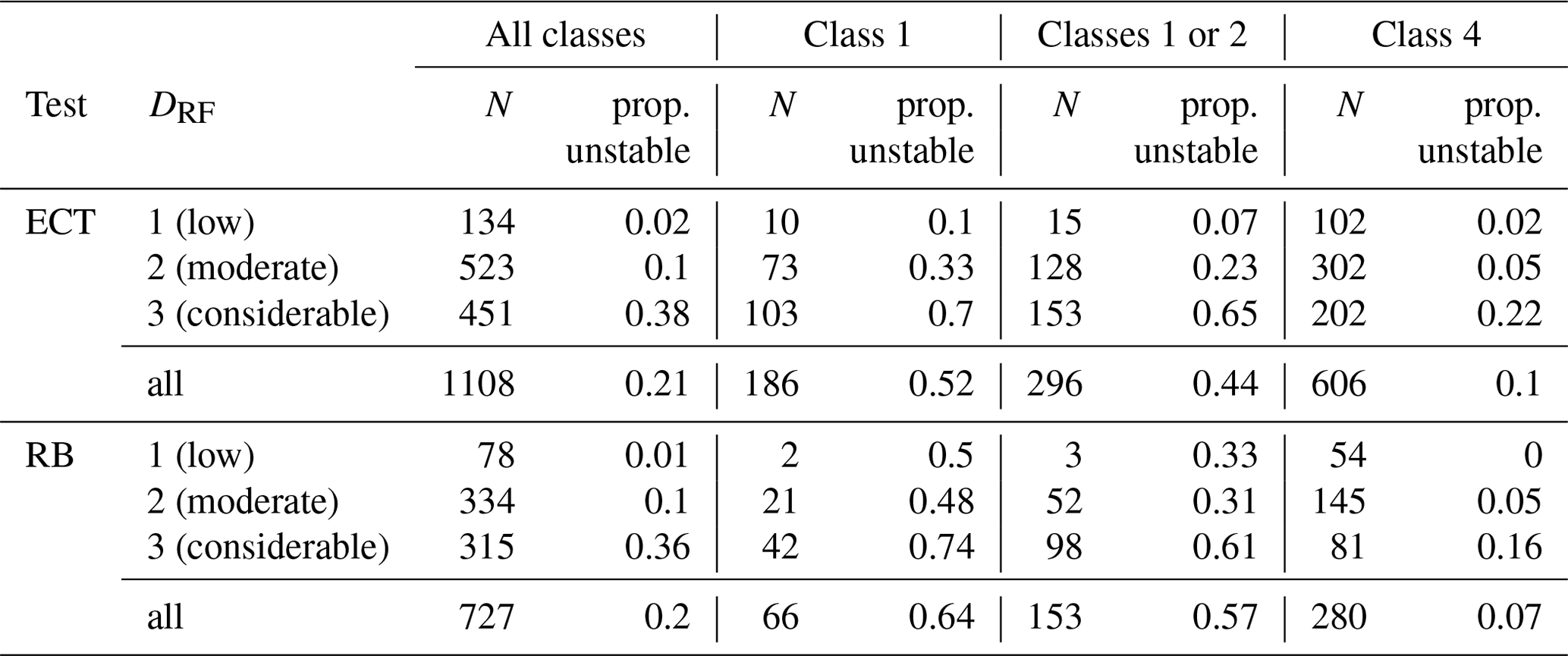
Considering a single ECT_new class 1 and RB class 1 showed that the proportion of unstable slopes (PPV) was always higher than the base rate proportion (Fig. 5), indicating that the stability test predicted a higher probability for the slope to be unstable than just assuming the base rate. This shift was more pronounced for the rutschblock test than for the ECT, particularly at level 1 (low) and 2 (moderate). The proportion of unstable slopes for ECT_new class 1 remained low at level 1 (low) and 2 (moderate) (proportion of unstable slopes ≤0.33, Table 4), indicating that it was still more likely that the slope was stable rather than unstable given such a test result (Table 4).

Figure 5 Proportion of unstable slopes (position of labels, RB – rutschblock test, ECT – single ECT_new) are shown compared to the respective base rate proportion of unstable slopes (black dots and black dashed line) for danger levels 1 (low), 2 (moderate), and 3 (considerable), as well as for the entire data set (all). The proportion of unstable values are shown for the respective lowest (red colour, labels above base rate line) and highest stability classes (blue, labels below base rate line).

Figure 5 also shows the shift in the proportion of unstable slopes (1−NPV) when considering ECT_new or RB stability class 4 (high stability). In these slopes, the proportion of unstable slopes was lower than the base rate, indicating that the probability the specific slope tested to be unstable was less than the base rate. The resulting proportion of unstable slopes was still higher compared to the base rate proportion of unstable slopes of the neighbouring next lower danger level.

Analysing the entire data set together, regardless of the forecast danger level, the proportion of unstable slopes was 0.21 and thus somewhat between the values for level 2 (moderate) and level 3 (considerable). Again, the informative value of the test can be noted (Fig. 5). However, ignoring the specific base rate related to a certain danger level leads – for instance – to an underestimation of the likelihood that the slope is unstable at level 3 (considerable) (RB or ECT_new class 1) or an overestimation for the presence of instability at level 1 (low) (RB or ECT_new class 4).

At level 1 (low), observations of RB stability class 1 were much less common (3 %, or 2 out of 78 tests, Table 4) compared to ECT_new class 1 (7 %). Similar observations were noted for classes 1 or 2: at level 1 (low) 4 % of the RB and 11 % of the ECT fell into these categories, increasing to 31 % (RB) and 34 % (ECT) of the tests at level 3 (considerable). This shift from the base rate proportion of unstable slopes to the observed proportion was more pronounced for the RB compared to the ECT.

As shown in Fig. 3c, the two extreme RB stability classes correlated better with slope stability than the respective two extreme ECT_new classes. This is also reflected in Fig. 5 by the stronger shift from the base rate proportion of unstable slopes to the observed proportion of unstable slopes. It is important to note that a stability test indicating stability class 4 was observed in 10 % (ECT) or 7 % (RB) of the cases in slopes rated unstable. This clearly emphasizes that a single stability test should never be trusted as the single decisive piece of evidence indicating stability.

5 Discussion

5.1 Performance of ECT classifications

We compared ECT results with concurrent slope stability information, applying existing classifications and testing a new one.

Quite clearly, whether a crack propagates across the entire column or not is the key discriminator between unstable and stable slopes (Fig. 3b). This is in line with previous studies (e.g. Simenhois and Birkeland, 2006; Moner et al., 2008; Simenhois and Birkeland, 2009; Winkler and Schweizer, 2009; Techel et al., 2016) and with our current understanding of avalanche formation (Schweizer et al., 2008b). Moreover, our results confirm the proposition by Winkler and Schweizer (2009) that the number of taps provides additional information allowing a better distinction between results related to stable and unstable conditions. The optimal threshold to achieve a balanced performance, i.e. high sensitivity as well as high specificity, was found to be between ECTP20 and ECTP22, depending on the method (k-means clustering, pROC cutoff point). This finding agrees well with the threshold proposed by Winkler and Schweizer (2009), who suggested ECTP21. Using the binary classification, as originally proposed by Simenhois and Birkeland (2009), increased the sensitivity but led to a rather high false-alarm rate. Moving away from a binary classification increased PPV and NPV for the lowest and highest stability classes, respectively, but came at the cost (or benefit) of introducing intermediate stability classes.

Only in some situations did pairs of ECTs performed in the same snow pit show an improved correlation with slope stability: when two tests were either ECT_new stability class 1 or 2, or when both tests were class 4, or one class 3 and one class 4.

5.2 Comparing ECT and RB

To our knowledge, and based on the review by Schweizer and Jamieson (2010), there have only been three previous studies that compared ECT and RB in the same data set.

Moner et al. (2008), in the Spanish Pyrenees, relying on a comparably small data set of 63 RBs (base rate 0.44) and 47 single ECTs (base rate 0.38) observed a higher unweighted average accuracy for the ECT (0.93) than the RB (0.88). In contrast, Winkler and Schweizer (2009, N=146, base rate 0.25) presented very similar values for the RB (0.84) and the ECT (0.81). However, Winkler and Schweizer (2009) partially relied on a slope stability classification which is based strongly on the rutschblock test. Therefore, they emphasized that the RB was favoured in their analysis. And, finally, the data presented by Techel et al. (2016) is to a large degree incorporated in the study presented here.

In that respect, this study presents the first comparison incorporating a comparably large number of ECTs and RBs conducted in the same snow pit, where slope stability was defined independently of test results. Seen from the perspective of the proportion of unstable slopes, the lowest and highest RB classes correlated better with slope stability than the respective ECT classes. Incorporating the sensitivity, the proportion of unstable slopes detected by a test, a mixed picture showed: that the single ECT and RB (classes 1 and 2) detected a comparable proportion of unstable slopes (0.56 vs. 0.53, respectively, Fig. 4c, d). Missed unstable classifications, however, were comparably rare for the RB (0.13) compared to a single ECT (0.21). Similar findings were noted for stable cases and stability class 4: RB results indicating instability on stable slopes (0.13) were less frequent than ECT indicating instability on stable slopes (0.27).

5.3 Predictive value of stability tests

We recall the three lessons drawn by Ebert (2019) in his theoretical investigation of the predictive value of stability tests using Bayesian reasoning in avalanche terrain, as this inspired us to explore these aspects using actual observations and compare them to our results:

1. “A localised diagnostic test will be more informative the higher the general avalanche warning” (Ebert, 2019, p. 4). With general “avalanche warning” Ebert (2019) referred to the forecast danger level as a proxy to estimate the base rate. As shown in Fig. 5, the observed proportion of unstable slopes (PPV) increased for both ECT and RB class 1 with increasing danger level, and hence base rate, supporting this statement.

2. “Do not `blame' the stability tests for false positive results: they are to be expected when the avalanche danger is low. In fact, their existence is a consequence of the basic fact that low-probability events are difficult to detect reliably” (Ebert, 2019, p. 4). Figure 5 supports this statement: at level 1 (low) and level 2 (moderate) an ECT indicating instability (class 1) was much more often observed on a stable slope than an unstable one. Only once the base rate proportion of unstable slopes was sufficiently high, in our case at level 3 (considerable), were tests indicating instability observed more often on unstable rather than stable slopes. When the base rate was low, the predictive value of the RB was higher than that of the ECT, suggesting that it may be worthwhile to invest the time required to perform a RB rather than an ECT.

3. “In avalanche decision-making, there is no certainty, all we can do is to apply tests to reduce the risk of a bad outcome, yet there will always be a residual risk” (Ebert, 2019, p. 5). The proportion of unstable slopes (PPV) was greater than the base rate proportion of unstable slopes for tests indicating instability, regardless of whether we considered an ECT or a RB result and regardless of the danger level, while the proportion of unstable slopes (or 1−NPV) was lower for tests indicating stability. From a Bayesian perspective, we can say that a positive test (a low-stability class) always increases our belief that the slope is unstable and vice versa when a test is negative (a high-stability class). In summary, both instability tests are useful despite the uncertainty which remains.

5.4 Sources of error and uncertainties

Besides potential misclassifications in slope stability, which we address more specifically in the following section (Sect. 5.5), Schweizer and Jamieson (2010) pointed out two other sources of error. The first of these is linked to the test methods, which are relatively crude methods and where, for instance, the loading may vary depending on the observer. The second error source is linked to the spatial variability of the snowpack. The constellation of slab and underlying weak layer properties vary in the terrain and may consequently have an impact on the test result. Furthermore, this data set did not permit us to check whether the failure layer of avalanches or whumpfs was linked to the failure layer observed in test results. Such information about the “critical weak layer” was, for instance, incorporated by Simenhois and Birkeland (2009) and Birkeland and Chabot (2006) in their analyses. However, from a stability perspective, considering the actual test result is the more relevant information.

5.5 Influence of the reference class definitions and the base rate

So far we have explored ECT and RB assuming that there are no misclassifications of slope stability. However, as the true slope stability is often not known (particularly in stable cases), errors in slope stability classification will occur. Such errors, however, may potentially influence all the statistics derived to describe the performance of tests (Brenner and Gefeller, 1997). For instance, if there are at least some slopes misclassified, classification performance will drop. However, in such cases, POD and PON will additionally be influenced by the true (though unknown) base rate (Brenner and Gefeller, 1997).

In previous studies exploring ECT (Moner et al., 2008; Simenhois and Birkeland, 2009; Winkler and Schweizer, 2009), slope stability classifications were generally well described and the base rate for the applied slope stability classification was given. However, slope stability classification approaches differed somewhat. For instance, a stability criterion used by Moner et al. (2008) was the occurrence of an avalanche on the test slope, while Simenhois and Birkeland (2009) additionally considered explosive testing of the slope as relevant information. Winkler and Schweizer (2009), on the other hand, additionally considered the manual profile classification used operationally in the Swiss avalanche warning service (Schweizer and Wiesinger, 2001; Schweizer, 2007). They already considered a location as unstable, when profiles were rated as very poor or poor. As this classification relies rather strongly on the RB result, the RB would be favoured in such an analysis (Winkler and Schweizer, 2009).

We have no knowledge about the uncertainty linked to our classification. However, we can demonstrate the impact of variations in the definition of the reference class on summary statistics like POD and PON, as well as using different data subsets for analysis: let us assume we are not interested in comparing ECT and RB but want to explore only the performance of a binary ECT classification with ECTP22 as the threshold between two classes. We will, however, use the RB together with the criteria introduced in Sect. 2.3 to define slope stability:

• Without using the RB as an additional criterion, POD and PON for the ECT was 0.56 and 0.79, respectively (Fig. 4c).

• If slopes were only considered to be unstable when the RB stability class was ≤2, and those with RB stability class 4 were considered to be stable, the resulting POD was 0.70 and PON was 0.91. The base rate in this data set was 0.32 and N=243.

• Being even more restrictive, and considering only slopes to be unstable when the RB stability class was 1, and those with RB stability class 4 considered to be stable, the resulting POD was 0.74 and PON was 0.91. The base rate in this data set was 0.2 and N=206.

Of course, one could also be interested in exploring the performance of a binary classification of the RB and define slope stability by using ECT results as an additional criterion to those in Sect. 2.3. Without relying on ECT results, POD and PON for the RB were 0.53 and 0.88, respectively (Fig. 4d). Considering only slopes to be unstable when additionally ECT_new stability class ≤ 2 was observed, and those with ECT_new class 4 as stable, POD and PON would increase to 0.66 and 0.94 (N=307, base rate 0.29), or 0.71 and 0.94, respectively when considering only ECT_new stability class 1 as unstable and class 4 as stable (N=285, base rate 0.23).

The combination of various error sources (Sect. 5.4), together with varying definitions of slope stability and differences in the base rate, make it almost impossible to directly compare results obtained in different studies. Therefore, performance values presented in this study, but also in other studies regarding snow instability tests, must always be seen in light of the specific data set used and allow primarily a comparison within the study.

5.6 Proposing stability class labels

For the purposes of this paper, we introduced class numbers to assign a clear order to the classes rather than assign class labels. However, the introduction of class labels rather than class numbers may ease the communication of results.

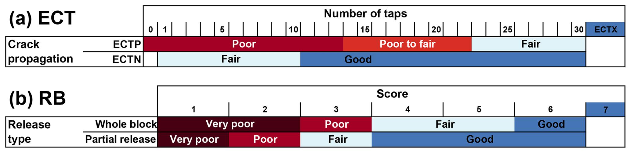
Figure 6 Proposed class labels for (a) ECT results based on crack propagation and number of taps with four classes: poor, poor to fair, fair and good. In panel (b) the RB classification is shown (same as in Fig. 2 but with four class labels).

We believe suitable terms should follow the established labelling for snow stability, which includes the main classes: poor, fair and good (e.g. CAA, 2014; Greene et al., 2016; Schweizer and Wiesinger, 2001). Hence, we suggest the following four stability class labels to rate the ECT results (Fig. 6a):

• poor – ECTP ≤13

• poor to fair – ECTP >13 to ECTP ≤22

• fair – ECTP >22 or ECTN ≤10

• good – ECTN >10.

Introducing these four labels allows an approximate alignment with the labels used for the RB (Fig. 6b) and reflects the variations in the proportion of unstable slopes observed between classes (Fig. 3c; proportion of unstable slopes for the four RB classes: 0.76, 0.53, 0.25 and 0.11, respectively; and proportion of unstable slopes for the four ECT classes: 0.6, 0.4, 0.27 and 0.16, respectively).

6 Conclusions

We explored a large data set of concurrent RB and ECT and related these to slope stability information. Our findings confirmed the well-known fact that crack propagation propensity, as observed with the ECT, is a key indicator relating to snow instability. The number of taps required to initiate a crack provides additional information concerning snow instability. Combining crack propagation propensity and the number of taps required to initiate a failure allows refining the original binary stability classification. Based on these findings, we propose an ECT stability interpretation with four distinctly different stability classes. This classification increased the agreement between slope stability and test result for the lowest (poor) and highest (good) stability classes compared to previous classification approaches. However, in our data set, the proportion of unstable slopes was higher and lower in the lowest and highest stability class, respectively, for the RB than for the ECT, regardless of whether one or two tests were performed. Hence, the RB correlated better with slope stability than the ECT. Performing a second ECT in the same snow pit increased the classification accuracy of the ECT only slightly. A second ECT performed in the same snow pit may be decisive for the highest or lowest classes that are best related with rather stable or unstable conditions, respectively, only when an ECT result was in one of the two intermediate classes.

We discussed further that changing the definition of the reference standard, the slope stability classification, has a large impact on summary statistics like POD or PON. This hinders comparison between studies, as differences in study designs, data selection and classification must be considered.

Finally, we investigated the predictive value of stability test results using a data-driven perspective. We conclude by rephrasing Blume (2002): when a stability test indicates instability, this is always statistical evidence of instability, as this will increase the likelihood for instability compared to the base rate. However, in cases of a low base rate, false-unstable predictions are likely.