the Creative Commons Attribution 4.0 License.
the Creative Commons Attribution 4.0 License.
 | 26 Apr 2019
Assessing the impact of sea surface temperatures on a simulated medicane using ensemble simulations
Robin Noyelle
Uwe Ulbrich
Nico Becker
Edmund P. Meredith
The sensitivity of the October 1996 Medicane in the western Mediterranean basin to sea surface temperatures (SSTs) is investigated with a regional climate model via ensemble sensitivity simulations. For 11 SST states, ranging from −4 K below to +6 K above the observed SST field (in 1 K steps), 24-member ensembles of the medicane are simulated. By using a modified phase space diagram and a simple compositing method, it is shown that the SST state has a minor influence on the tracks of the cyclones but a strong influence on their intensities. Increased SSTs lead to greater probabilities of tropical transitions, to stronger lower- and upper-level warm cores and to lower pressure minima. The tropical transition occurs sooner and lasts longer, which enables a greater number of transitioning cyclones to survive landfall over Sardinia and re-intensify in the Tyrrhenian Sea. The results demonstrate that SSTs influence the intensity of fluxes from the sea, which leads to greater convective activity before the storms reach their maturity. These results suggest that the processes at steady state for medicanes are very similar to tropical cyclones.
- Article
(3173 KB) - Full-text XML
- BibTeX
- EndNote


The Mediterranean basin is one of the most cyclogenetic regions in the world, with a majority of its cyclones being baroclinic (Wernli and Schwierz, 2006). However, it has been shown since the 1960s, using remote sensing instruments, that unusual cyclones with a visual similarity to tropical cyclones are also sometimes observed (Ernst and Matson, 1983; Mayengon, 1984; Rasmussen and Zick, 1987). In contrast to asymmetric, synoptic-scale extratropical cyclones, these cyclones are of a smaller scale, axisymmetric, frontless and sometimes have a well-defined eye at their center. These cyclones are now referred to as tropical-like Mediterranean cyclones, or medicanes. According to the climatological study of Cavicchia et al. (2014a), over the last 60 years medicanes have occurred with a frequency of 1.57±1.30 events per year.
Medicanes are intense low-pressure systems that present similar characteristics to tropical cyclones: an area with no cloud at the center, spiral bands surrounded by deep convection, intense surface winds, a lower- and upper-troposphere warm core, formation over the sea, and a rapid dissipation after landfall (Pytharoulis, 2018). In recent decades, thanks to high-resolution regional numerical weather prediction models and observational data, detailed examinations of several medicane cases have been carried out (e.g., Reale and Atlas, 2001; Chaboureau et al., 2012; Miglietta et al., 2013, 2017; Tous and Romero, 2013; Tous et al., 2013; Picornell et al., 2013; Miglietta et al., 2015; Cioni et al., 2016).
The question of the influence of sea surface temperatures (SSTs) on the development and the characteristics of medicanes has been tackled by several studies. Reed et al. (2001) found a minor influence of small SST anomalies on the medicane of 23 January 1982. Homar et al. (2003) showed that the development scenario of the medicane of 12 September 1996 had many similarities with the air–sea interaction instability mechanism, especially with the latent heat fluxes acting as a sustainer of convection. According to them, the medicane would have been both weaker and had a delayed development if the SSTs had been colder. Fita et al. (2007) showed the strong sensitivity of the same medicane to SSTs using an axisymmetric cloud-resolving model in which other environmental influences were not included. Miglietta et al. (2011) studied the impact of systematic changing of SSTs in a simulation of the 26 September 2006 medicane. According to them, the cyclone was mainly sensitive to uniform SST changes larger than 2 K and increasingly lost its tropical features as the SSTs became colder. Pytharoulis (2018) investigated the influence of SSTs on the 7 November 2014 Medicane through the imposition of climatological SSTs and uniform warm and cold SST anomalies. A linear deepening and a longer lifetime of the medicane were observed as the SST anomalies increased from −3 to +1 K.
The October 1996 Medicane was previously studied by Mazza et al. (2017), using a 50-member ensemble of regional climate model simulations. It was shown that standard extratropical dynamics were responsible for the cyclogenesis and that the tropical transition of the cyclone resulted from a warm seclusion process. Our present study aims to assess the role of SSTs in the development and the intensity of this cyclone. Ensembles are created for different SST states through dynamical downscaling of reanalysis data and applying a uniform change to the observed SST field in a range of −4 to +6 K. As such, we seek to assess the sensitivity of the medicane to a range of SST changes extending well beyond observational uncertainty and to instead consider SST changes in ranges more typically associated with natural or externally forced variability. To identify any potential threshold and/or nonlinear behavior in the system, we further extend the SST states to encompass the range −4 to +6 K. To the best of our knowledge, ours is the first study to use ensemble simulations combined with uniform SST changes to evaluate the influence of SSTs on the formation of a particular medicane.
Section 2 provides an overview of the medicane case, while Sect. 3 describes the model setup and methodology. Results are presented in Sect. 4, while the discussion and conclusions are included in Sect. 5.
In this paper we study Medicane Cornelia, which occurred in the western Mediterranean between 7 and 10 October 1996. The cyclone is discussed in detail in Reale and Atlas (2001) and Cavicchia and von Storch (2012), with a synthesized description of the case in Mazza et al. (2017). Here we provide an abridged overview of the case.
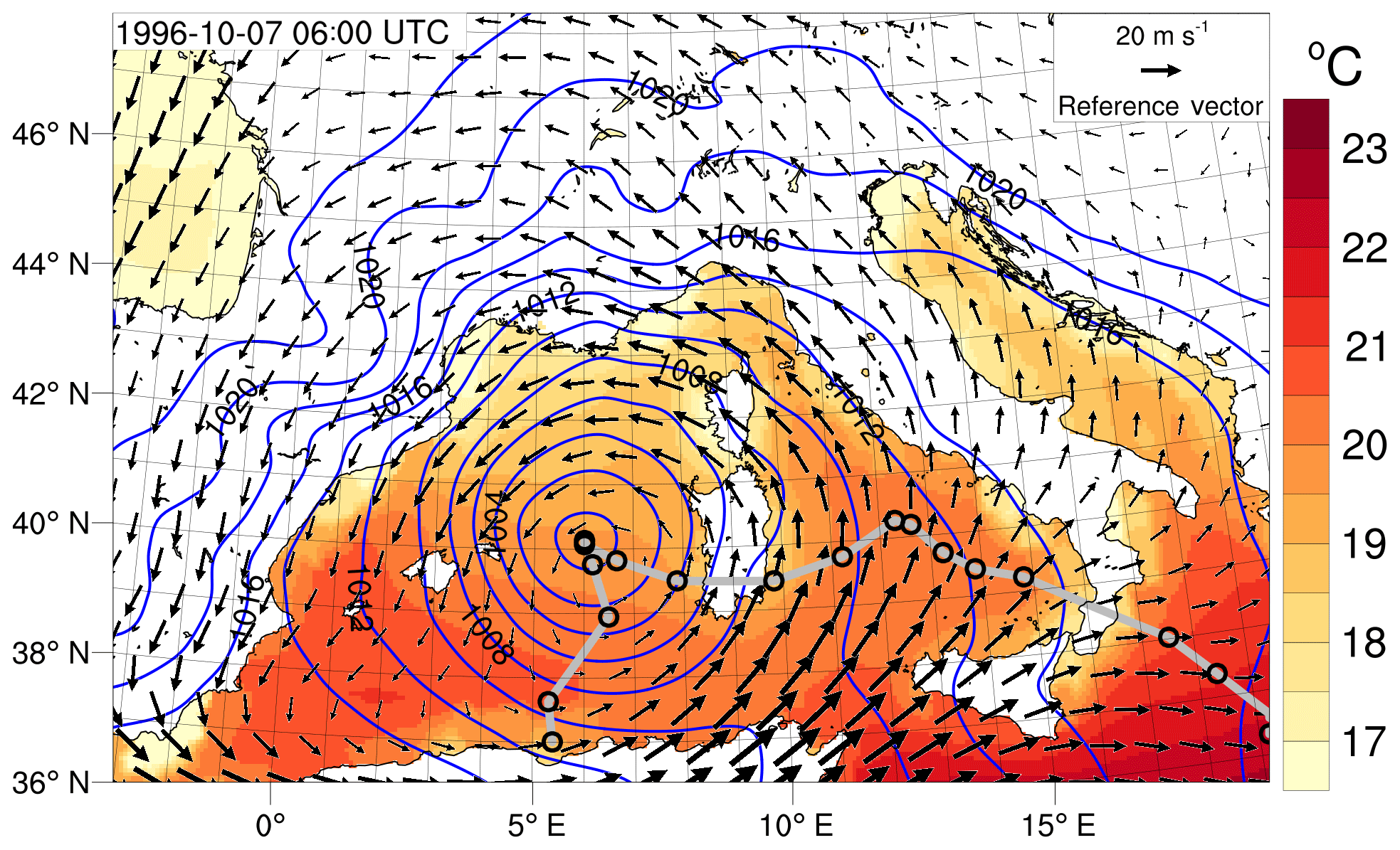
Figure 1Inner simulation domain (0.0625∘ resolution) and medicane in reanalysis. SSTs (shading), sea level pressure (hPa, blue contours) and 500 hPa wind vectors, representative of the steering flow, are shown for 7 October 1996 at 06:00 UTC. The cyclone's track is shown with a grey line, marked at 6 h intervals from 6 October 1996 at 06:00 UTC. The plot is based on ERA-Interim data.
Medicane Cornelia began its life as an extratropical cyclone with frontal structures on 6 October 1996 near the Algerian coast. By 12:00 UTC on 7 October it had tracked northwards, guided by the steering flow of a 500 hPa cutoff low, to lie between the Balearic Islands and Sardinia. A clear eye-like structure was present by this stage (Mazza et al., 2017), and the central pressure had deepened below 1000 hPa (Reale and Atlas, 2001) with SSTs close to 20 ∘C (Fig. 1). From here Cornelia tracked eastwards, crossing Sardinia on 8 October and weakening over land, before re-intensifying as it tracked east into the Tyrrhenian Sea (Cavicchia and von Storch, 2012). By 9 October the medicane was situated north of Sicily, with the central vortex having become more intense and compact (Reale and Atlas, 2001). Cornelia then tracked southeastwards, crossing Calabria on the night of 9 October, where intense winds were recorded, before dissipating in the Ionian Sea during 10 October (Reale and Atlas, 2001).
3.1 Experimental setup
The numerical simulations are performed with the full-physics, non-hydrostatic COSMO Climate Limited-Area Model (CCLM; Rockel et al., 2008) version cosmo4.8-clm19. CCLM is the community model of the German regional climate research community jointly developed further by the CLM community. The two-step downscaling configuration begins with a 257×271 grid point, 0.165∘ resolution parent domain, which is forced at the lateral boundaries by ERA-Interim reanalysis (Dee et al., 2011). A 288×192 grid point, 0.0625∘ resolution domain (Fig. 1) is then nested within the 0.165∘ parent domain; the 0.165∘ domain covers an area slightly smaller than the EURO-CORDEX domain (Jacob et al., 2014) and is shown in Mazza et al. (2017). For both downscaling steps, the model setup includes an extended microphysics scheme accounting for cloud water and cloud ice for grid scale precipitation, based on Kessler (1969), the Ritter and Geleyn (1992) radiation scheme, and the Tiedtke parameterization scheme for convection (Tiedtke, 1989). Heat fluxes from the ocean to the atmosphere are parameterized using a stability-, roughness-length-dependent surface flux formulation based on Louis (1979). Both domains feature 40 vertical levels and a 6-hourly update of the boundary conditions. One ensemble is performed, driven by the 0.7∘ resolution ERA-Interim reanalysis (Dee et al., 2011).
3.2 Ensemble generation
According to previous studies (Davolio et al., 2009; Chaboureau et al., 2012; Cioni et al., 2016; Mazza et al., 2017), numerical forecasts are highly sensitive to initial and boundary conditions. In particular, the location of the lateral boundaries can have a strong impact on circulation anomalies within the model domain (e.g., Miguez-Macho et al., 2004; Becker et al., 2018). In this study, the technique of domain shifting is employed to generate an ensemble (Pardowitz et al., 2016). This technique consists of two downscaling steps with a series of simulations that have domains that are slightly shifted in space. We use the same procedure as in Mazza et al. (2017).
-
The first downscaling step entails the following:
-
locating a central domain over Europe (same as in Mazza et al., 2017),
-
shifting the central domain in terms of longitude and latitude in eight directions (north, south, east, west, northeast, northwest, southeast and southwest) in three steps (0.25, 0.50 and 0.75∘),
-
running the model on each of the 24 domains using ERA-Interim as initial and boundary conditions.
-
-
The second downscaling step entails the following:
-
using the 24 simulations of the first downscaling step as initial and boundary conditions for the smaller, nested domain (Fig. 1) with a finer resolution over the western and central Mediterranean basin.
-
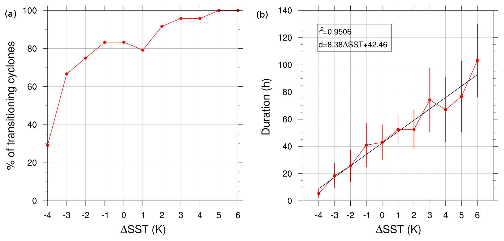
Figure 2(a) Percentage of cyclones encountering a tropical transition over the 24-member ensembles for different SST changes, using classification criteria based on the cyclone phase space. (b) Mean period of time during which transitioning cyclones are classified as medicanes for different SST changes. Error bars represent standard deviation. The black line is based on a linear regression.
This results in one set of 24 simulations for the reference (observed) SSTs from ERA-Interim. It is important to emphasize that all choices of domain boundaries are equally valid and that the central “unshifted” domain is not the “correct” domain. Any simulated differences between the ensemble members are thus a consequence of the inherent uncertainty resulting from forcing the regional model with imperfect boundary conditions (i.e., reanalysis) and the chaotic nature in which the system responds to differences in the lateral boundary conditions. As such, the potential subsequent formation of a medicane should always be considered in a probabilistic rather than a deterministic manner. Simulated characteristics of the medicane (e.g., its track) must thus also be interpreted in a statistical sense, and the ensemble mean characteristics may not correspond exactly to the observed characteristics, which are themselves just one of many potential realizations.
As in Mazza et al. (2017), the initialization time of the first step simulations is 00:00 UTC on 1 October 1996, while the inner domains are initialized at 00:00 UTC on 4 October 1996. A 72 h lag was previously found to be a satisfactory compromise between introducing sufficient spread in the ensemble and the ability to capture the event in the simulations (Mazza et al., 2017).
3.3 SST changes
To assess the sensitivity of the October 1996 Medicane to SSTs, we perturb the SST forcing in the 0.0625∘ domain by adding SST anomalies in a range of −4 to +6 K, in 1 K increments, to the observed SST field. In addition to the ensemble using observed SSTs, this creates 10 extra 24-member ensembles relating to our chosen case, each with their own unique SST forcing. SSTs were modified uniformly across the entire 0.0625∘ domain.
3.4 Cyclone phase space
We base our analyses on the three-dimensional diagnostics proposed by Hart (2003), which were first applied to the study of medicanes by Chaboureau et al. (2012), and subsequently by others (Miglietta et al., 2013; Mazza et al., 2017), to analyze medicane tropical transition. The three following parameters are computed in a radius of 150 km from the cyclone's center (as successfully used by Mazza et al., 2017) and are used to define the cyclone phase space.
-
The thermal symmetry in the lower troposphere (B) is the difference in mean 600–900 hPa thickness between the left and right semicircles with respect to the cyclone's trajectory.
-
The lower-tropospheric thermal wind () is the vertical derivative of the cyclone's geopotential height perturbation between 900 and 600 hPa.
-
The upper-tropospheric thermal wind () is the vertical derivative of the cyclone's geopotential height perturbation between 600 and 400 hPa.
The exact definitions that we use for these parameters represent a modified version of the diagnostics proposed by Hart (2003), which take into account the limited vertical extent and the smaller spatial scale of medicanes compared to tropical cyclones (Picornell et al., 2013; Miglietta et al., 2013; Cioni et al., 2016; Mazza et al., 2017). Our exploration radius is thus reduced from 500 to 150 km and the upper bound of is reduced from 300 to 400 hPa. The resulting phase space diagrams can be very erratic on an hourly timescale. Therefore, a 3 h running mean is applied to the computed parameters to give the final phase space diagram. Following Hart (2003), in order to classify a cyclone as a medicane, the following objective criteria must apply simultaneously at least one time step: B<10 m, and .
3.5 Cyclone tracking
The simulated cyclones are tracked based on the mean sea level pressure (MSLP). As hourly data were used, this proved to be sufficient to correctly follow the cyclone track. The tracking algorithm works as follows.
-
Initially, the location of the minimum pressure is identified within the area of the western Mediterranean basin at 00:00 UTC on 8 October; at that point in time the cyclone is fully developed with a core pressure below 1013 hPa, is located over Sardinia and is found in every simulation.
-
The positions of the MSLP minima in the adjacent time steps (backward and forward in time) are determined using a nearest-neighbor algorithm, applied within a circle with a radius of 0.9∘ from the previous MSLP minimum.
-
The algorithm stops if the cyclone's minimum pressure exceeds 1013 hPa or has made landfall on the French or Spanish coastline (Corsica, Sardinia, Sicily and continental Italy are not considered as landfall).
-
Every track is verified manually with respect to its consistency with the MSLP fields.
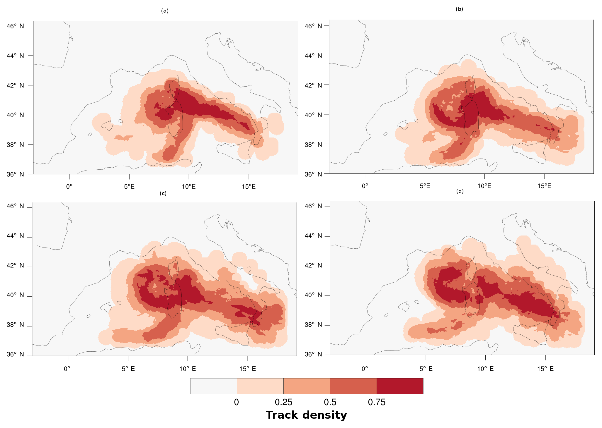
Figure 3Track densities based on all cyclones for an SST change of (a) −3 K, (b) 0 K (original SSTs), (c) +3 K and (d) +6 K.
This algorithm gives coherent trajectories for cyclones both with and without a tropical transition. The algorithm ensures that only one cyclone track is identified in each ensemble member. Continental Italy is not considered as landfall in order to follow the medicanes even when they make landfall; this is done in order to specifically calculate the evolution of the phase space parameters after landfall. In practice, medicanes dissipate rapidly after landfall.
This method gives reasonable tracks during most of the cyclone's lifetime, which allows the computation of the phase space parameters. In the early phase of the cyclone the tracks can be slightly erratic. However, this does not affect the results because this period is before the earliest stage of the cyclone's life used for composite analysis (20 h before the time of maximum warm-core strength; see Sect. 3.6). The phase space parameter B could significantly change with a more sophisticated tracking algorithm because it is sensitive to the exact location of the track position. While our method of distinguishing a medicane from a non-medicane requires that all criteria mentioned in Sect. 3.4 are fulfilled simultaneously, for the systems considered in this study the evaluation of alone would have led to the same systems being identified.
Track density plots are obtained by counting, for each grid point, the number of tracks that cross a 50 km radius circle around the respective grid point for all members of a given SST ensemble, and dividing by the total number of tracks (see Kruschke et al., 2016, for a similar method applied to Northern Hemisphere winter storms).
3.6 Cyclone compositing
In order to extract the mean signal from fields that show large variability, we use a simple arithmetic-averaging technique called cyclone compositing. This technique has been frequently applied to both extratropical and tropical cyclones (e.g., Frank, 1977; Bracken and Bosart, 2000; Bengtsson et al., 2007; Catto et al., 2010; Mazza et al., 2017). Following Mazza et al. (2017), we align the temporal evolution of the simulated cyclones to a common reference time: for each track we identify the time step when is at its maximum, B<10 m and . This instant is meant to reflect the stage of maximum warm-core strength and is hence referred to as the maximum warm-core time (MWCT). Such an instant is found for all cyclones analyzed in this study, even non-transitioning ones. As we focus on transitioning cyclones, for studying mechanisms it proves most instructive to base our analyses on composites of the 10 most powerful transitioning cyclones for each SST, i.e., those that have the greatest at MWCT (except when ∘C because for this SST state only 7 cyclones transition). Results are insensitive to whether we take the mean or median of the composited cyclones.
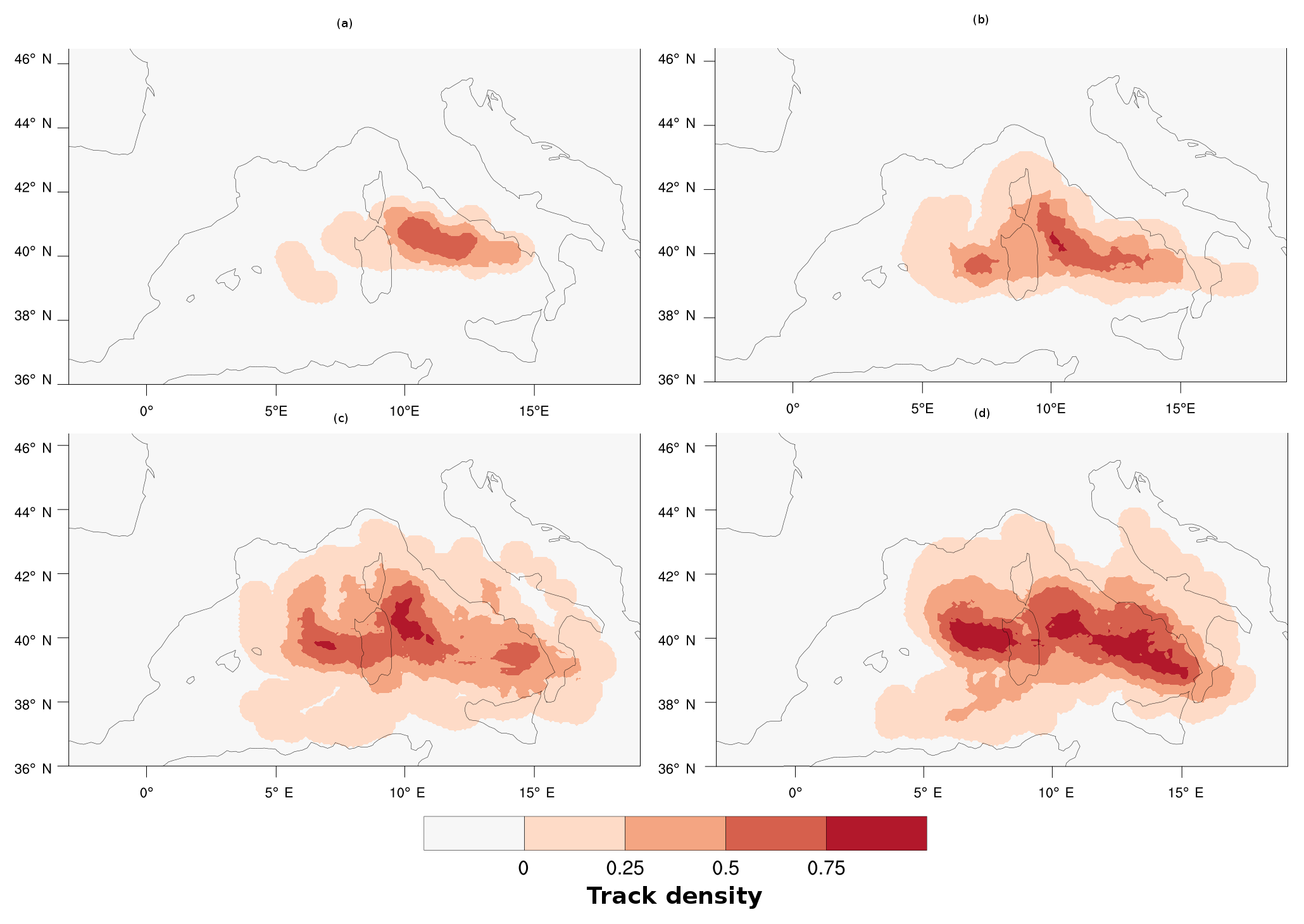
Figure 4Track densities based on all cyclones classified as medicanes for an SST change of (a) −3 K, (b) 0 K (original SSTs), (c) +3 K and (d) +6 K.
4.1 Probability of transition and track density
With the specified criteria based on the phase space parameters, it can be determined if a cyclone undergoes a tropical transition, i.e., if it can be regarded as a medicane. This is done for each of the 24 ensemble members of each of the 11 SST states. It is found that increasing SST leads to an increasing number of medicanes (Fig. 2a). While at K only 30 % of the ensemble members generate a transitioning cyclone, at +5 and +6 K all members produce a medicane. Note that even with observed SSTs, i.e., ΔSST=0 K, medicane transition probability is less than 85 %. This points towards the probabilistic nature of medicane formation: the observed medicane was one of many potential realizations for the observed SST state; small changes in the observed initial conditions could have developed to inhibit the real-world formation of Medicane Cornelia as well. The largest increase in medicane development rate is found between −4 and −3 K (from 7 to 16 medicanes). It could be speculated that this sudden increase is related to a specific SST threshold, similar to the empirical threshold of 26.5 ∘C, which is found for the development of tropical cyclones (Gray, 1968). However, here the SSTs are much lower (around 20 ∘C).
From each ensemble, those cyclones that are classified as a medicane are selected. For this subset, the mean and standard deviation of the period of time during which the cyclone was classified as a medicane are calculated. The length of this period increases almost linearly with increasing SSTs (Fig. 2b). For an SST change of −4 K, the period of time is very short, with values of around 5 h. In contrast, the period of time lasts longer at higher SSTs. For example, at K the cyclones are classified as medicanes for about 104 h on average. Not only the mean but also the standard deviation between the time periods in the different ensemble members increases with increasing SSTs.
Figure 3 presents track densities of cyclones for an SST change of −3, 0, +3 and +6 K. The figure must be viewed taking into account that cyclones begin to form between Sardinia and the Balearic Islands, then move through Sardinia and finally go southeast of the Tyrrhenian Sea. All track density plots are very similar when SSTs change and it only seems to be a greater dispersion of tracks when we increase SSTs, especially east of Sardinia and south of continental Italy. Therefore, one can conclude that the SST state has little influence on the track of the medicane, with the large-scale steering flow instead playing the dominant role.
However, Fig. 4 shows the track densities obtained with the same method, but tracks are taken into account only when cyclones are classified as medicanes. The two local maxima of density east and west of Sardinia illustrate that the simulations exhibit two distinct classes of medicane formation: those for which MWCT occurs before crossing Sardinia and weaken after the crossing and those for which MWCT occurs after crossing Sardinia, mostly near the Italian peninsula, and continue to deepen after the crossing. It is observed that between 60 % and 85 % of the medicanes are of the second type, depending on the SST change. However, there is no systematic dependency between the observed percentage and ΔSST. While some medicanes of the first type that lose their medicane status while crossing Sardinia go on to re-transition in the Tyrrhenian Sea, others fail to regain medicane status. In addition to this, many medicanes of the second type first achieve medicane status in the Tyrrhenian Sea, as suggested by the two local maxima. Figure 4 also shows that, apart from increasing the period of time when cyclones are transitioning, the track is always similar: the first transition is before Sardinia, then crossing Sardinia and finally moving southeast to Calabria through the Tyrrhenian Sea. Even if the variability increases with higher SSTs, it seems that tracks are not SST-dependent.
4.2 Intensity of the cyclones
As a first step, the intensities of the cyclones are analyzed in terms of the minimum core pressure. For this purpose, the composite (see Sect. 3.6) sea level pressure minimum (i.e., the mean of the 10 pressure minima from the tracks of the 10 cyclones that have the greatest at MWCT) is calculated for each ΔSST. The composite mean of the minimum MSLP decreases from 1004 hPa at −4 K to 981 hPa at +6 K, while the standard deviation, i.e., the variability, between the individual ensemble members strongly increases at higher SSTs (Fig. 5). A regression equation specification error test (Ramsey, 1969) showed that the null hypothesis that the relationship between ΔSST and minimum MSLP is linear can be rejected at a significance level of 0.01. That means that there is a nonlinear relationship between SSTs and the minimum pressure of the medicanes. SSTs seem to act as an amplifying factor of an already existing minimum pressure caused by a higher tropospheric feature.
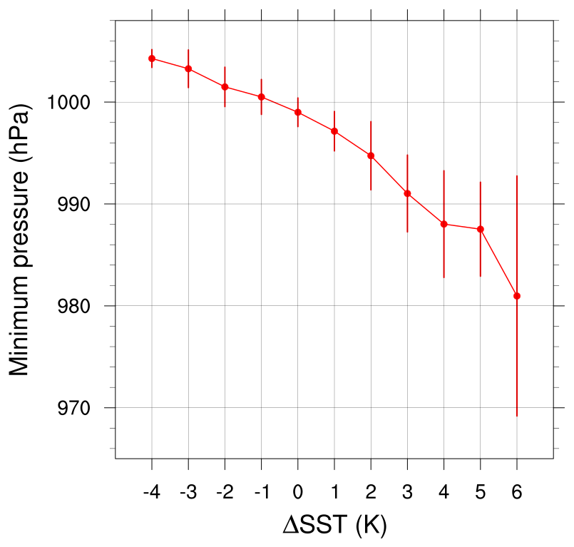
Figure 5Dependence of composite minimum pressure on SST change. The error bars represent standard deviation.
As the SSTs are not uniformly distributed in the Mediterranean Sea, one may ask whether the differences between the different realizations of the cyclone are caused by differences in the local SSTs along the specific cyclone tracks of the individual ensemble members. To assess the role of local SSTs along the cyclone tracks, we calculate the mean SSTs in a radius of 150 km around the cyclone center and take the average of those values from MWCT −20 h until MWCT for each track. These average SST values are presented together with the minimum pressure for all ensemble members of all SST states (including non-transitioning cyclones) in Fig. 6. For each SST state, the local SSTs encountered by all cyclones before MWCT vary in the range of 1 K around a mean value. In each ensemble the local SSTs along the cyclone track are thus roughly similar. The minimum pressure, however, can still vary considerably. For example, at +6 K the simulated values of minimum pressure range from 954 to 1002 hPa. In addition to this, we also find that there are certain ensemble members, i.e., those with particular domain shifts that enter the 10-member composites more often than others across the range of SST states. Taken together, these findings indicate that while there is a clear tendency towards more intense medicanes at higher SSTs, higher SSTs are not the sole criterion for an intense medicane. A mesoscale environment supportive of rapid intensification and tropical transition is also crucial, and local SSTs are not sufficient to fully account for the variability of the cyclones' minimum pressure.
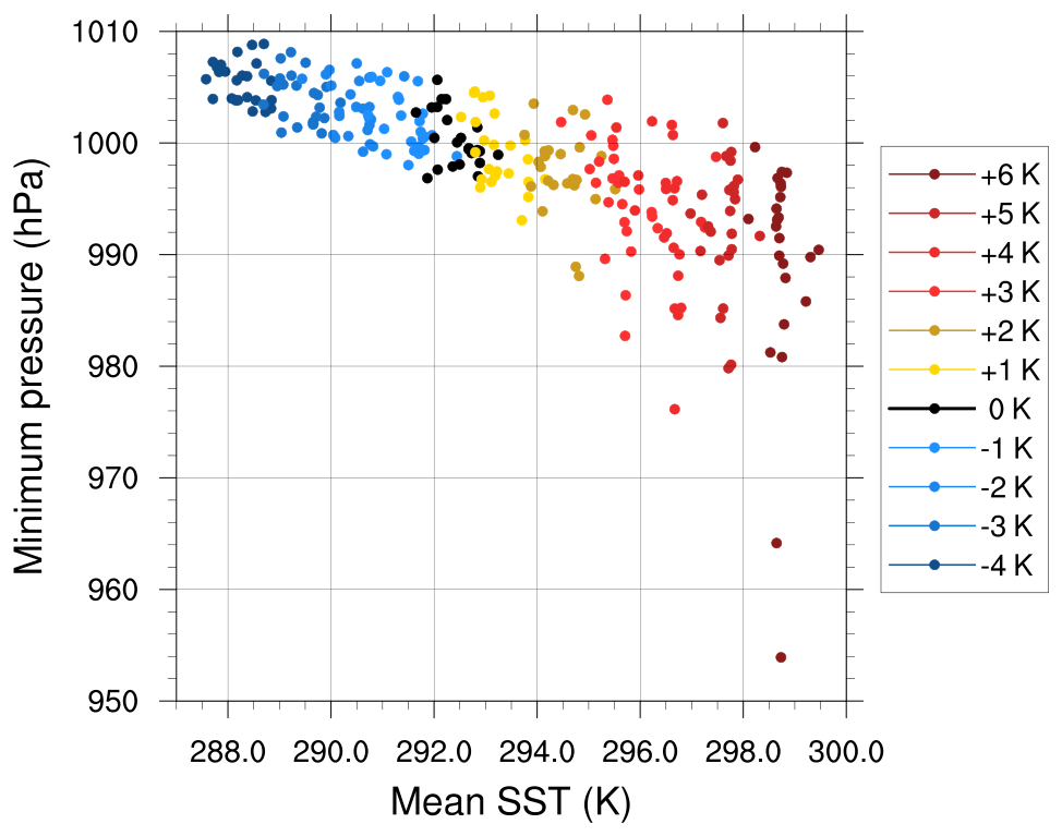
Figure 6Dependence of minimum pressure on mean SST in a radius of 150 km, as encountered by the cyclone from −20 h before MWCT until MWCT. Colors represent global SST change. Note that this plot is based on all cyclones and is not a composite average.
Figure 7 shows the temporal evolution of the composite minimum of sea level pressure for all ΔSST from −20 h before to +10 h after MWCT. The curves are almost equally spaced at −20 h, but they diverge as MWCT is approaching and reach a minimum at MWCT for almost all SST states. It is evident that at higher SSTs medicane transition and deepening begins earlier, the deepening rate is larger and the medicanes retain their tropical-like structure longer compared to at lower SSTs (Figs. 7, A1 in the Appendix).
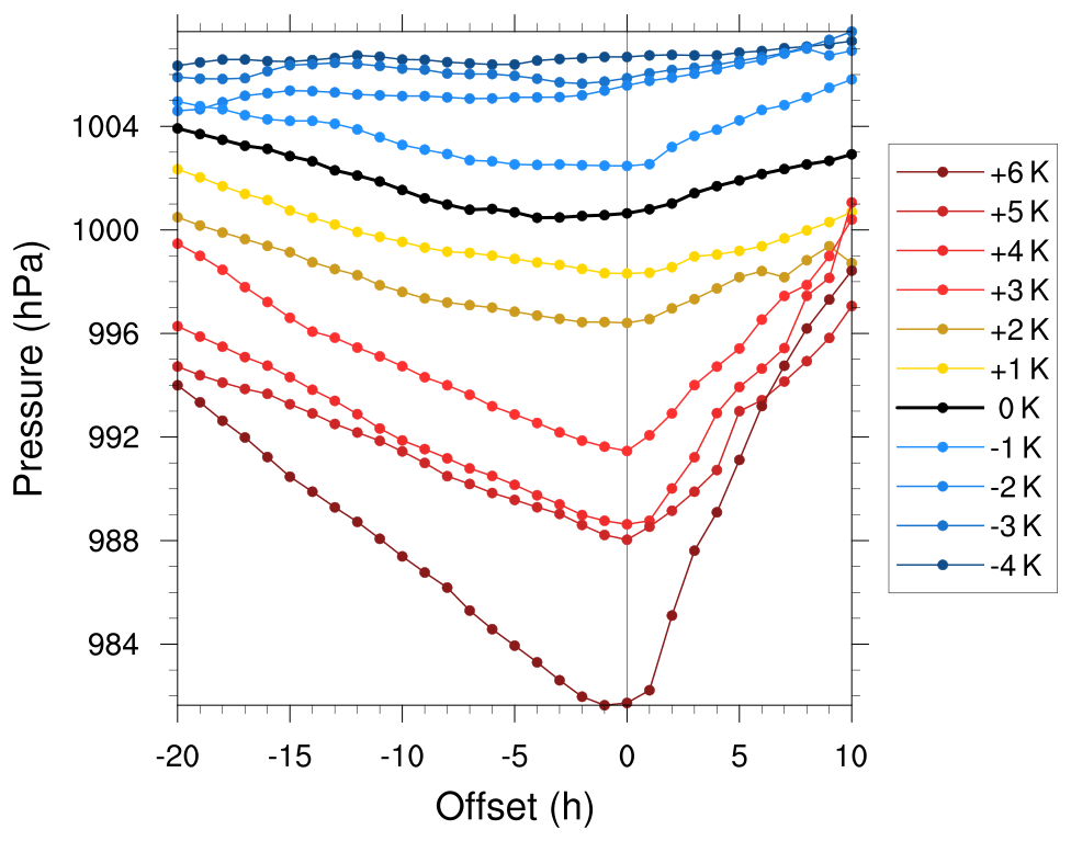
Figure 7Composite time series of minimum pressure from −20 h before until +10 h after MWCT for each SST change.
It is observed that the phase space parameters and at MWCT increase linearly with increasing SSTs (Fig. 8). It is obvious that medicanes get stronger when SSTs increase, as the thermal winds between 600 and 900 hPa and 400 and 600 hPa at MWCT increase in almost the same proportion. Figure 9 presents the temporal evolution of the composite of those two parameters from −20 h before to +10 h after MWCT for each ΔSST. There is a roughly parallel evolution for each ΔSST for the parameter with similar rates of increase. This contrasts with the evolution of minimum pressure, which showed different rates for different ΔSST (Fig. 7). The evolution for the parameter is more erratic but, at least for positive SST changes, the observation is similar. Regressing the hourly magnitudes of and against each other in the period MWCT −20 h to MWCT separately for each SST state composite reveals greater differences in the magnitudes of and at colder SST states. This suggests the development of a deeper medicane warm core with higher thermal coherence in the warmer SST composites, likely generated by enhanced upper-level latent heat release from more intense convective updrafts at higher SSTs (Fig. 10).
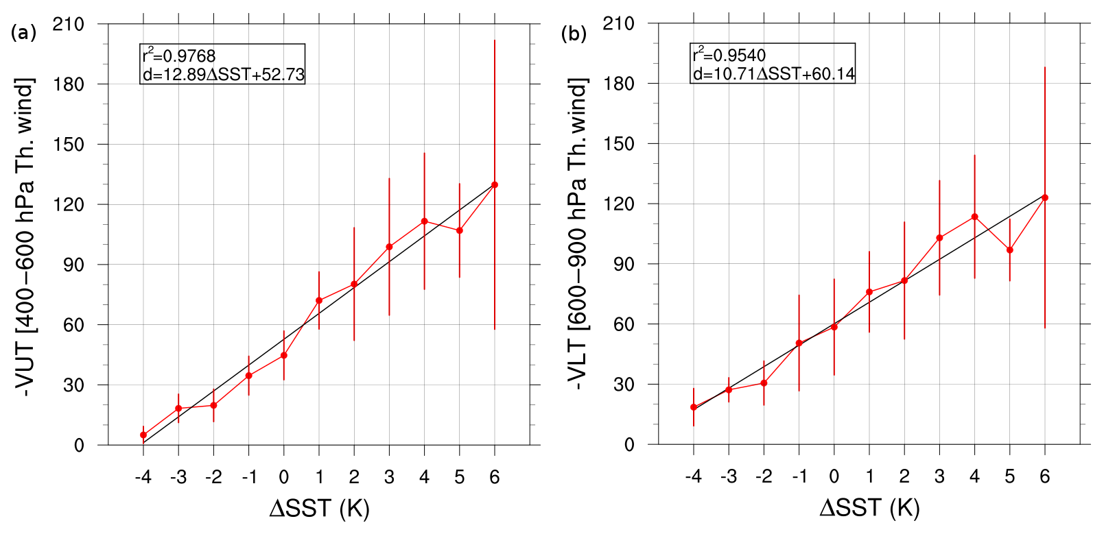
Figure 8Dependence of composite of (a) and (b) at MWCT on SST change. The error bars represent standard deviation.
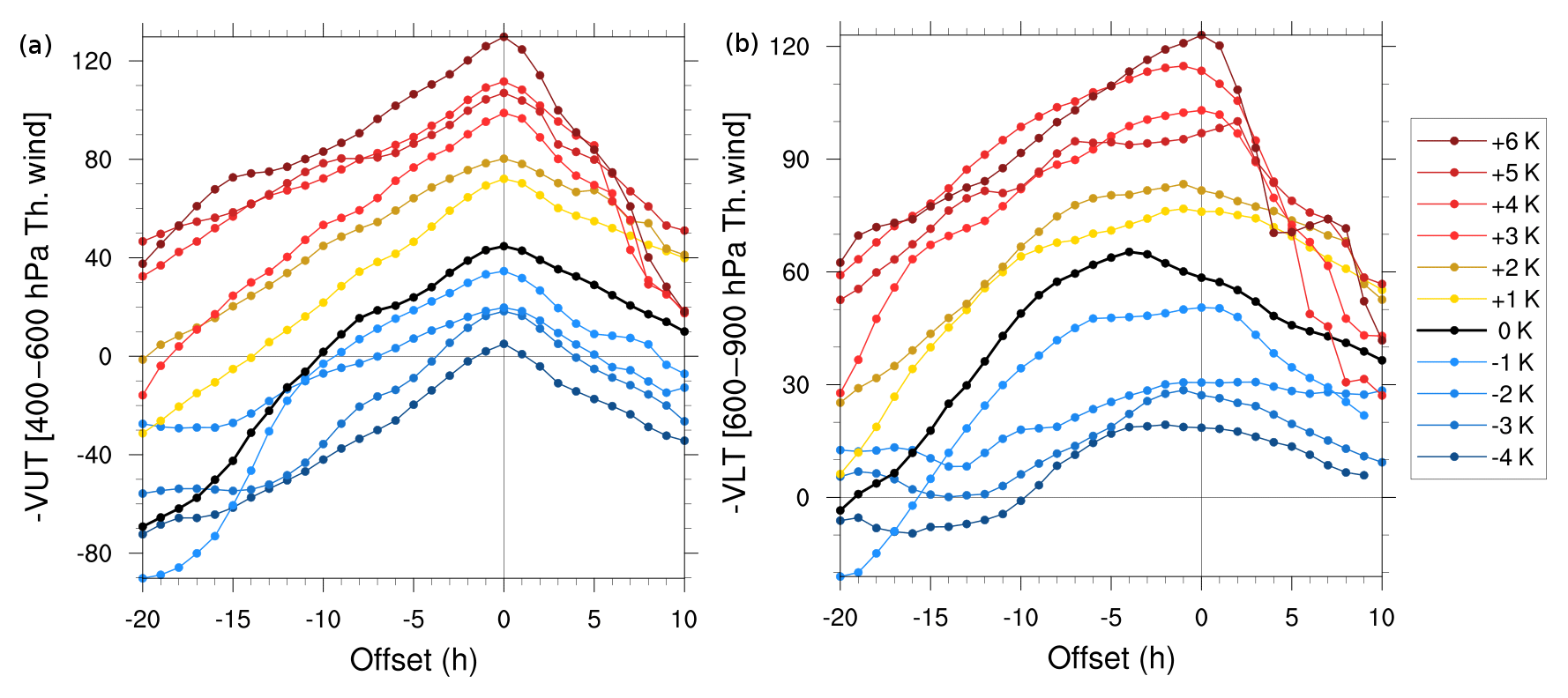
Figure 9Composite time series of (a) and (b) from −20 h before to +10 h after MWCT for each SST change.
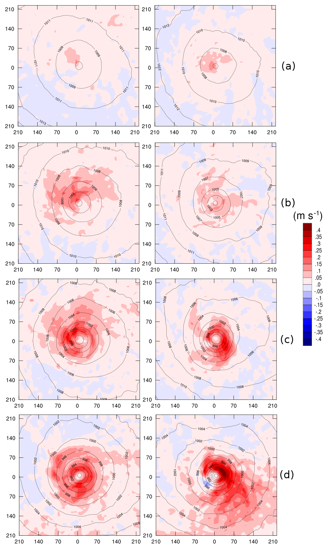
Figure 10The 10 h mean of composite vertical wind speed at 500 hPa for an SST change of (a) −3 K, (b) 0 K (original SSTs), (c) +3 K and (d) +6 K (colors), as well as composite mean sea level pressure (contours) between MWCT −20 h and MWCT −10 h (left column) and between MWCT −10 h and MWCT (right column). The values on the x and y axis indicate the distance from the center of the medicane in kilometers.
4.3 The influence of the fluxes from the sea
Similar to tropical cyclones, the main source of potential energy of medicanes is the thermodynamic disequilibrium between the atmosphere and the underlying sea surface. Therefore, it is generally accepted that there is a direct relationship between SST and cyclone intensity (Miglietta et al., 2011). The prescribed SST changes directly affect the sensible and latent heat fluxes from the ocean into the atmospheric boundary layer. To analyze the heat fluxes under different SST conditions, the composite structure of the latent heat fluxes from the sea are computed 20 and 10 h before MWCT, and at MWCT. The horizontal structure of the medicane is remarkably well defined for and +6 K, with strong gradients of pressure near the center of the cyclone, very low heat fluxes in the eye region and the strongest heat fluxes of more than 400 W m2 in a radius between 50 and 100 km around the center (Fig. 11). This structure is consistent with the air–sea interaction proposed by Emanuel (1986) for tropical cyclones. It is worth noting that the horizontal structure of the fluxes is not perfectly symmetrical, which is caused by the surrounding islands and continental land area. In particular, there are systematically weaker fluxes northeast of the composite medicane. This effect is the imprint of continental Italy, which is characterized by considerably lower latent heat fluxes than the ocean areas.
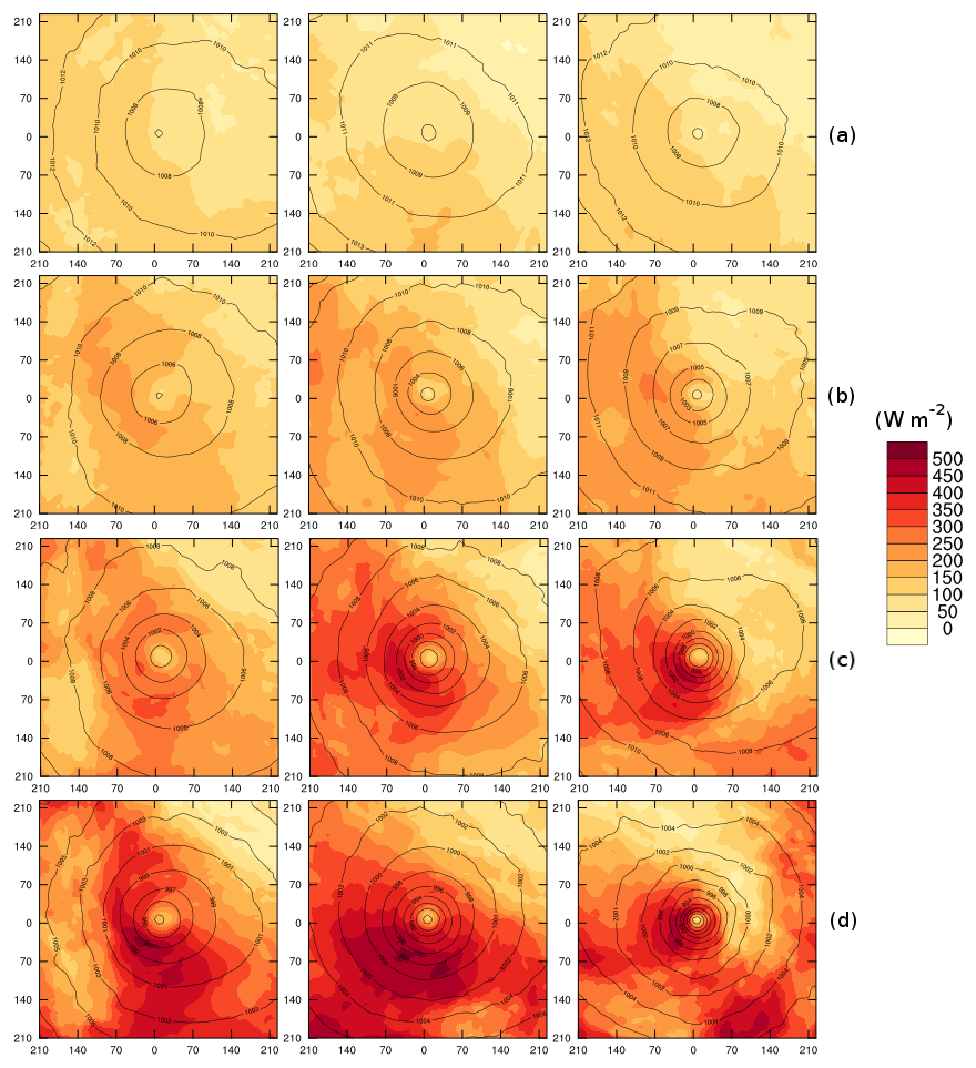
Figure 11Composite latent heat fluxes from the sea for an SST change of (a) −3 K, (b) 0 K (original SSTs), (c) +3 K and (d) +6 K (colors), as well as composite mean sea level pressure (contours) at MWCT −20 h (left column), MWCT −10 h (center column) and MWCT (right column). The values on the x and y axis indicate the distance from the center of the medicane in kilometers.
For K there is no well-defined spatial structure in the composite heat fluxes and the heat fluxes are very low with values below 150 W m2 (Fig. 11a). Nevertheless, the cyclones of this composite are classified as a medicane based on the phase space parameters. Therefore, the fluxes from the sea might play a minor role in the formation of those medicanes.
In composites of vertical cross sections around the cyclone centers, the vertical wind speeds were analyzed (not shown). It was found that the largest vertical wind speeds occur in the middle troposphere around 500 hPa. Figure 10 shows the 10 h mean of the vertical wind speeds at the 500 hPa level of the composite medicane and its evolution before MWCT. Maximum vertical wind speeds occur around 50 km away from the center of the cyclone, similar to the strongest heat fluxes. This reflects the development of deep convection in the entire troposphere, i.e., the deepening process that leads to the intensification of the medicane. As in the case of the heat fluxes, the intensity of the vertical wind speeds increases with increasing SSTs.
As one would expect, fluxes from the sea are higher when SSTs increase, leading to greater vertical wind speeds and hence more intense deep convection throughout the troposphere. This in turn leads to a more intense deepening of the medicane and stronger sea level pressure gradients, thus more intense medicanes. This chain of processes is coherent with the classical model of Emanuel (1986) for the steady state of tropical cyclones.
In this study the sensitivity of a simulated medicane in the western Mediterranean to SSTs was analyzed in an ensemble of full-physics, non-hydrostatic regional model simulations with COSMO-CLM. In the first downscaling step, 24-member ensembles were created by systematic shifts of the model domain. In the second downscaling step with a horizontal resolution of 0.0625∘, SSTs were changed uniformly by adding SST anomalies (in a range of −4 to +6 K in 1 K increments) to the observed SST field, creating eleven 24-member ensembles.
The cyclones were analyzed and classified according to a modified cyclone phase space following Hart (2003). For each SST change, out of the transitioning cyclones, the 10 cyclones featuring the strongest upper-level warm cores were composited (except when K because there are only 7 transitioning cyclones; see Sect. 3.6).
It was shown that the number of transitioning cyclones increases with increasing SSTs. A particularly strong increase was found between and −3 K, which corresponds to average SST values of around 16 ∘C within the area of medicane development. These results support the idea that a threshold exists for tropical-like cyclones in the Mediterranean Sea, similar to tropical cyclones (Gray, 1968). Miglietta et al. (2011) suggested that, as the presence of medicanes is associated with cold-air intrusions, they can form even when the SSTs are below the threshold of 26.5 ∘C for tropical cyclones. Similarly, the duration of the transition increased almost linearly with SSTs. The cyclone tracks showed small random variations in the different ensemble members. However, the tracks of the cyclones, with or without tropical transition, showed no systematic dependency on SSTs compared to the control situation (ΔSST=0 K). This suggests that the track characteristics depend on the large-scale dynamics of the upper-level low, which determines the environmental steering conditions relevant for the movement of the medicane.
Once the mesoscale environment is conducive to tropical transition and the formation of a strong medicane, medicane intensity depends strongly on SSTs, as found in our composites. The composite medicane's minimum pressure decreases when SSTs increase, following a nonlinear relationship, in contrast to the intensity of its lower- and upper-troposphere warm core, which follow the linear evolution of the duration of the medicane. The process of transitioning is roughly similar when SSTs change, except that the cyclones transition earlier and are less affected by orography when crossing Sardinia. As SSTs increase, the sensible and latent heat fluxes from the sea into the atmosphere increase. The vertical wind speeds in a region of 50 km around the eye of the medicane also increase, which can be explained by an intensification of deep convection processes caused by the increased heat fluxes. This deep convection leads to deeper sea level pressure minima, stronger pressure gradients and upper-level warm cores, which occur at the same time just before the medicanes make landfall and begin to dissipate.
Miglietta et al. (2011) found in a similar study of uniform SST changes that the sensible and latent heat fluxes from the sea surface during the transit of the cyclone across the Mediterranean Sea have the effect of modifying the boundary layer and are thus efficient mechanisms for convective destabilization. They concluded that warmer (colder) SSTs produce stronger (weaker) sea surface fluxes, favoring an earlier (delayed) removal of convective inhibition and enhancing (reducing) the development of convection and the intensification of the cyclone. The results of our study, using ensemble simulations, are in strong agreement with these conclusions. They also concluded that the critical SST anomaly for which the atmospheric circulation displays the characteristics of the actually observed medicane is about K. Even though we did not compare our results to the observed phenomenon and the situation they studied is located further south than ours, therefore showing higher SSTs of 1 to 2 ∘C, we also find that a critical value for the appearance of medicanes is around K. Pytharoulis (2018) found an almost linear deepening of the medicane and an increasing lifetime as the SST anomalies increased from −3 to +1 K. A nonlinearity was, however, found as even warmer SST anomalies were applied: a weaker medicane was simulated and this was mainly attributed to the lack of a well-defined upper-air warm core. A nonlinearity was also found at warmer SSTs in our study but only for minimum pressure and in the direction of deepening and not weakening.
It is clear that our approach using prescribed SST changes can not fully simulate the impact of SSTs on the development of a medicane, since feedback processes from the medicane to the ocean are not taken into account. In particular, our modeling strategy reflects Atmospheric Model Intercomparison Project (AMIP)-style studies, in which the complexity of ocean–atmosphere interactions is removed from the modeling process by prescribing SSTs as a lower boundary condition (Gates, 1992). This allows a clear but rather idealized attribution of the observed effects to the applied SST changes. It should be noted that the inflow into the computational domain is not changed, thus producing a large difference between SSTs and air temperatures close to the lateral boundaries. Furthermore, strong gradients are also induced between SSTs and land temperatures. However, the temperatures over land, and coastal areas in particular, were proven to adapt rapidly to the SST changes before the formation of the cyclone. Ricchi et al. (2017) studied the impact of the modeling approach (with or without ocean–atmosphere coupling) on simulated medicanes and found the medicane tracks and intensities to exhibit little sensitivity. Akhtar et al. (2014), meanwhile, studied the robustness of COSMO-CLM coupled with a one-dimensional ocean model (1-D NEMO-MED12). They showed that at high resolution, the coupled model is able to not only simulate most medicane events but also improve the track length, core temperature and wind speed of simulated medicanes compared to the atmosphere-only simulations, suggesting that the coupled model is more proficient for systematic and detailed studies of historical medicane events. It would be valuable to assess the role of SSTs with such a coupled model.
With climate change, in the last decades of the 21st century (2070–2099) the SSTs of the Mediterranean Sea are projected to increase by 1.73 to 2.97 K relative to 1961–1990 (Adloff et al., 2015). Similarly to Pytharoulis (2018), the results of this study suggest that if the upper-air conditions of the atmosphere remain unchanged, stronger and longer-lasting medicanes than today will appear more frequently in the Mediterranean basin. However, the development of medicanes is influenced by additional factors like the presence of baroclinic instability or a cold cutoff low in the upper atmospheric layers. It is likely that climate change will also affect these factors. Romero and Emanuel (2013) and Cavicchia et al. (2014b) both showed that the intensity of medicanes is projected to increase, while their frequency will decrease. Ensemble sensitivity studies, such as those presented here, are thus a valuable tool for offering insights into how the life cycles of medicanes may differ in a warmer climate.
Information about the availability of the COSMO-CLM source code can be found at https://www.clm-community.eu (last access: 14 April 2019). The simulation data generated as part of this work have been archived at the DKRZ World Data Center for Climate (https://www.dkrz.de/up/systems/wdcc, last access: 14 April 2019), are publicly available under an open-access license (http://cera-www.dkrz.de/WDCC/ui/Compact.jsp?acronym=DKRZ_LTA_961_ds00005, last access: 14 April 2019) and citable as Noyelle et al. (2018). Researchers interested in scientific collaboration and/or data usage are asked to contact the authors.
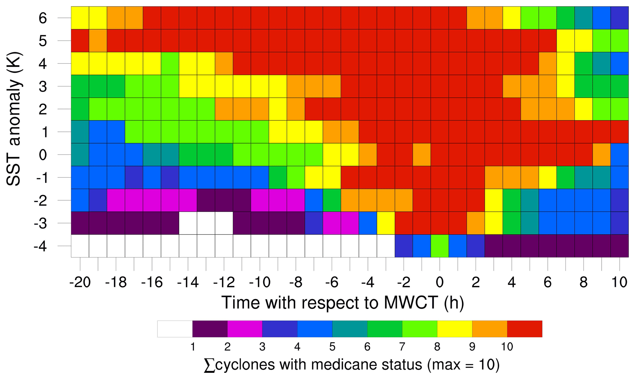
Figure A1Number of medicanes in each composite (one composite per SST state, y axis) that have medicane status at a given time relative to MWCT. Note that each composite contains 10 members, except for the −4 K anomaly SST composite, which contains only 7 members as only 7 members underwent transition.
RN performed the analysis and simulations and wrote the manuscript. EM and NB contributed to the analysis. All authors contributed to the writing of the manuscript and discussed the analysis and results.
The authors declare that they have no conflict of interest.
The computational resources were made available by the German Climate Computing Center (DKRZ). The authors would like to acknowledge the European Union for funding this research through an Erasmus+ scholarship. Robin Noyelle would like to thank Ingo Kirchner, Stefan Pfahl and Edoardo Mazza for their fruitful comments.
This paper was edited by Vassiliki Kotroni and reviewed by two anonymous referees.
Adloff, F., Somot, S., Sevault, F., Jordà, G., Aznar, R., Déqué, M., Herrmann, M., Marcos, M., Dubois, C., Padorno, E., Alvarez-Fanjul, E., and Gomis, D.: Mediterranean Sea response to climate change in an ensemble of twenty first century scenarios, Clim. Dynam., 45, 2775–2802, 2015. a
Akhtar, N., Brauch, J., Dobler, A., Béranger, K., and Ahrens, B.: Medicanes in an ocean–atmosphere coupled regional climate model, Nat. Hazards Earth Syst. Sci., 14, 2189–2201, https://doi.org/10.5194/nhess-14-2189-2014, 2014. a
Becker, N., Ulbrich, U., and Klein, R.: Large-scale secondary circulations in a limited area model–the impact of lateral boundaries and resolution, Tellus A, 70, 1–15, 2018. a
Bengtsson, L., Hodges, K. I., Esch, M., Keenlyside, N., Kornblueh, L., Luo, J.-J., and Yamagata, T.: How may tropical cyclones change in a warmer climate?, Tellus A, 59, 539–561, 2007. a
Bracken, W. E. and Bosart, L. F.: The role of synoptic-scale flow during tropical cyclogenesis over the North Atlantic Ocean, Mon. Weather Rev., 128, 353–376, 2000. a
Catto, J. L., Shaffrey, L. C., and Hodges, K. I.: Can climate models capture the structure of extratropical cyclones?, J. Climate, 23, 1621–1635, 2010. a
Cavicchia, L. and von Storch, H.: The simulation of medicanes in a high-resolution regional climate model, Clim. Dynam., 39, 2273–2290, 2012. a, b
Cavicchia, L., von Storch, H., and Gualdi, S.: A long-term climatology of medicanes, Clim. Dynam., 43, 1183–1195, 2014a. a
Cavicchia, L., von Storch, H., and Gualdi, S.: Mediterranean tropical-like cyclones in present and future climate, J. Climate, 27, 7493–7501, 2014b. a
Chaboureau, J.-P., Pantillon, F., Lambert, D., Richard, E., and Claud, C.: Tropical transition of a Mediterranean storm by jet crossing, Q. J. Roy. Meteor. Soc., 138, 596–611, 2012. a, b, c
Cioni, G., Malguzzi, P., and Buzzi, A.: Thermal structure and dynamical precursor of a Mediterranean tropical-like cyclone, Q. J. Roy. Meteor. Soc., 142, 1757–1766, 2016. a, b, c
Davolio, S., Miglietta, M. M., Moscatello, A., Pacifico, F., Buzzi, A., and Rotunno, R.: Numerical forecast and analysis of a tropical-like cyclone in the Ionian Sea, Nat. Hazards Earth Syst. Sci., 9, 551–562, https://doi.org/10.5194/nhess-9-551-2009, 2009. a
Dee, D. P., Uppala, S. M., Simmons, A. J., Berrisford, P., Poli, P., Kobayashi, S., Andrae, U., Balmaseda, M. A., Balsamo, G., Bauer, P., Bechtold, P., Beljaars, A. C. M., van de Berg, L., Bidlot, J., Bormann, N., Delsol, C., Dragani, R., Fuentes, M., Geer, A. J., Haimberger, L., Healy, S. B., Hersbach, H., Hólm, E. V., Isaksen, L., Kållberg, P., Köhler, M., Matricardi, M., McNally, A. P., Monge-Sanz, B. M., Morcrette, J.-J. Park, B.-K., Peubey, C., de Rosnay, P., Tavolato, C., Thépaut, J.-N., and Vitart, F.: The ERA-Interim reanalysis: Configuration and performance of the data assimilation system, Q. J. Roy. Meteor. Soc., 137, 553–597, 2011. a, b
Emanuel, K. A.: An air-sea interaction theory for tropical cyclones. Part I: Steady-state maintenance, J. Atmos. Sci., 43, 585–605, 1986. a, b
Ernst, J. and Matson, M.: A Mediterranean tropical storm?, Weather, 38, 332–337, 1983. a
Fita, L., Romero, R., Luque, A., Emanuel, K., and Ramis, C.: Analysis of the environments of seven Mediterranean tropical-like storms using an axisymmetric, nonhydrostatic, cloud resolving model, Nat. Hazards Earth Syst. Sci., 7, 41–56, https://doi.org/10.5194/nhess-7-41-2007, 2007. a
Frank, W. M.: The structure and energetics of the tropical cyclone I. Storm structure, Mon. Weather Rev., 105, 1119–1135, 1977. a
Gates, W. L.: AN AMS CONTINUING SERIES: GLOBAL CHANGE–AMIP: The Atmospheric Model Intercomparison Project, B. Am. Meteorol. Soc., 73, 1962–1970, 1992. a
Gray, W. M.: Global view of the origin of tropical disturbances and storms, Mon. Weather Rev., 96, 669–700, https://doi.org/10.1175/1520-0493(1968)096<0669:GVOTOO>2.0.CO;2, 1968. a, b
Hart, R. E.: A cyclone phase space derived from thermal wind and thermal asymmetry, Mon. Weather Rev., 131, 585–616, 2003. a, b, c, d
Homar, V., Romero, R., Stensrud, D., Ramis, C., and Alonso, S.: Numerical diagnosis of a small, quasi-tropical cyclone over the western Mediterranean: Dynamical vs. boundary factors, Q. J. Roy. Meteor. Soc., 129, 1469–1490, 2003. a
Jacob, D., Petersen, J., Eggert, B., Alias, A., Christensen, O. B., Bouwer, L. M., Braun, A., Colette, A., Déqué, M., Georgievski, G., Georgopoulou, E., Gobiet, A., Menut, L., Nikulin, G., Haensler, A., Hempelmann, N., Jones, C., Keuler, K., Kovats, S., Kröner, N., Kotlarski, S., Kriegsmann, A., Martin, E., van Meijgaard, E., Moseley, C., Pfeifer, S., Preuschmann, S., Radermacher, C., Radtke, K., Rechid, D., Rounsevell, M., Samuelsson, P., Somot, S., Soussana, J.-F., Teichmann, C., Valentini, R., Vautard, R., Weber, B., and Yiou, P.: EURO-CORDEX: new high-resolution climate change projections for European impact research, Reg. Environ. Change, 14, 563–578, https://doi.org/10.1007/s10113-013-0499-2, 2014. a
Kessler, E. (Ed.): On the distribution and continuity of water substance in atmospheric circulations, in: On the distribution and continuity of water substance in atmospheric circulations, 1–84, Springer, Boston, 1969. a
Kruschke, T., Rust, H. W., Kadow, C., Müller, W. A., Pohlmann, H., and Leckebusch, G. C.: Probabilistic evaluation of decadal prediction skill regarding Northern Hemisphere winter storms, Meteorol. Z., 25, 721–738, 2016. a
Louis, J.-F.: A parametric model of vertical eddy fluxes in the atmosphere, Bound.-Lay. Meteorol., 17, 187–202, 1979. a
Mayengon, R.: Warm core cyclones in the Mediterranean, Mariners Weather Log, 28, 6–9, 1984. a
Mazza, E., Ulbrich, U., and Klein, R.: The Tropical Transition of the October 1996 Medicane in the Western Mediterranean Sea: A Warm Seclusion Event, Mon. Weather Rev., 145, 2575–2595, 2017. a, b, c, d, e, f, g, h, i, j, k, l, m, n
Miglietta, M., Laviola, S., Malvaldi, A., Conte, D., Levizzani, V., and Price, C.: Analysis of tropical-like cyclones over the Mediterranean Sea through a combined modeling and satellite approach, Geophys. Res. Lett., 40, 2400–2405, 2013. a, b, c
Miglietta, M., Cerrai, D., Laviola, S., Cattani, E., and Levizzani, V.: Potential vorticity patterns in Mediterranean “hurricanes”, Geophys. Res. Lett., 44, 2537–2545, 2017. a
Miglietta, M. M., Moscatello, A., Conte, D., Mannarini, G., Lacorata, G., and Rotunno, R.: Numerical analysis of a Mediterranean “hurricane” over south-eastern Italy: sensitivity experiments to sea surface temperature, Atmos. Res., 101, 412–426, 2011. a, b, c, d
Miglietta, M. M., Mastrangelo, D., and Conte, D.: Influence of physics parameterization schemes on the simulation of a tropical-like cyclone in the Mediterranean Sea, Atmos. Res., 153, 360–375, 2015. a
Miguez-Macho, G., Stenchikov, G. L., and Robock, A.: Spectral nudging to eliminate the effects of domain position and geometry in regional climate model simulations, J. Geophys. Res.-Atmos., 109, D13, https://doi.org/10.1029/2003JD004495, 2004. a
Noyelle, R., Ulbrich, U., Becker, N., and Meredith, E. P.: Assessing the impact of SSTs on a simulated medicane using ensemble simulations, available at: http://cera-www.dkrz.de/WDCC/ui/Compact.jsp?acronym=DKRZ_LTA_961_ds00005 (last access: 14 April 2019), 2018. a
Pardowitz, T., Befort, D. J., Leckebusch, G. C., and Ulbrich, U.: Estimating uncertainties from high resolution simulations of extreme wind storms and consequences for impacts, Meteorol. Z., 25, 531–541, 2016. a
Picornell, M. A., Campins, J., and Jansà, A.: Detection and thermal description of medicanes from numerical simulation, Nat. Hazards Earth Syst. Sci., 14, 1059–1070, https://doi.org/10.5194/nhess-14-1059-2014, 2014. a, b
Pytharoulis, I.: Analysis of a Mediterranean tropical-like cyclone and its sensitivity to the sea surface temperatures, Atmos. Res., 208, 167–179, 2018. a, b, c, d
Ramsey, J. B.: Tests for specification errors in classical linear least-squares regression analysis, J. Roy. Stat. Soc. B Met., 31, 350–371, 1969. a
Rasmussen, E. and Zick, C.: A subsynoptic vortex over the Mediterranean with some resemblance to polar lows, Tellus A, 39, 408–425, 1987. a
Reale, O. and Atlas, R.: Tropical cyclone–like vortices in the extratropics: Observational evidence and synoptic analysis, Weather Forecast., 16, 7–34, 2001. a, b, c, d, e
Reed, R., Kuo, Y.-H., Albright, M., Gao, K., Guo, Y.-R., and Huang, W.: Analysis and modeling of a tropical-like cyclonein the Mediterranean Sea, Meteorol. Atmos. Phys., 76, 183–202, 2001. a
Ricchi, A., Miglietta, M., Barbariol, F., Benetazzo, A., Bergamasco, A., Bonaldo, D., Cassardo, C., Falcieri, F., Modugno, G., Russo, A., Sclavo, M., and Carniel, S.: Sensitivity of a Mediterranean tropical-like cyclone to different model configurations and coupling strategies, Atmosphere, 8, 92, https://doi.org/10.3390/atmos8050092, 2017. a
Ritter, B. and Geleyn, J.-F.: A comprehensive radiation scheme for numerical weather prediction models with potential applications in climate simulations, Mon. Weather Rev., 120, 303–325, 1992. a
Rockel, B., Will, A., and Hense, A.: The regional climate model COSMO-CLM (CCLM), Meteorol. Z., 17, 347–348, 2008. a
Romero, R. and Emanuel, K.: Medicane risk in a changing climate, J. Geophys. Res.-Atmos., 118, 5992–6001, 2013. a
Tiedtke, M.: A comprehensive mass flux scheme for cumulus parameterization in large-scale models, Mon. Weather Rev., 117, 1779–1800, 1989. a
Tous, M. and Romero, R.: Meteorological environments associated with medicane development, Int. J. Climatol., 33, 1–14, 2013. a
Tous, M., Romero, R., and Ramis, C.: Surface heat fluxes influence on medicane trajectories and intensification, Atmos. Res., 123, 400–411, 2013. a
Wernli, H. and Schwierz, C.: Surface cyclones in the ERA-40 dataset (1958–2001). Part I: Novel identification method and global climatology, J. Atmos. Sci., 63, 2486–2507, 2006. a